Article

Optimal On-Orbit Inspection of Satellite Formation

1
Department of Industrial Engineering, University of Bologna, I-47121 Forlì, Italy
2
Department of Civil and Industrial Engineering, University of Pisa, I-56122 Pisa, Italy
*
Author to whom correspondence should be addressed.
Remote Sens. 2022, 14(20), 5192; https://doi.org/10.3390/rs14205192
Submission received: 15 September 2022 / Revised: 10 October 2022 / Accepted: 16 October 2022 / Published: 17 October 2022

Abstract

:
In a formation-flying mission where multiple spacecraft must cooperate and maintain a prescribed relative separation, the early detection of possible anomalies is a primary requirement. This is possible, for example, by employing an inspector spacecraft whose aim is to monitor the condition of the formation members with an on-orbit inspection. This paper analyzes a rest-to-rest multiple-impulse transfer that the inspector spacecraft must accomplish to visit all of the formation members. The problem is studied using the linearized Hill–Clohessy–Wiltshire equations and is solved in an optimal framework by minimizing the total velocity variation along the transfer trajectory. The solution algorithm implements a two-step procedure that combines differential evolution algorithms and Nelder–Mead simplex method-based routines. A case study is thoroughly investigated where a formation of six satellites covers a circular orbit of altitude 300 km over Earth. The proposed algorithm could efficiently find a solution and with reduced computational times.

1. Introduction

Spacecraft formation flying is an interesting mission concept that has attracted much interest from the scientific community in the last few decades [1]. It basically consists of a network of satellites that collaborate with each other by sharing information and data to accomplish complex tasks that would be difficult to achieve with a single conventional spacecraft.
There are several space missions where the formation of two or more satellites is conceived to meet the mission requirements. For example, Gravity Recovery and Climate Experiment (GRACE) was a joint mission of NASA and DLR in which twin satellites (GRACE-1 and GRACE-2) took detailed measurements of Earth’s gravity field anomalies from March 2002 to October 2017 while being separated by a constant distance of 220 km along their own orbits. Another important example is the Swarm mission, which was launched by the European Space Agency (ESA) in 2013 with the purpose of studying Earth’s magnetic field. The Swarm constellation consisted of three satellites (Alpha, Bravo, and Charlie) placed in two different polar orbits: Alpha and Charlie f;ew side by side at an altitude of 450 km , and Bravo at an altitude of 530 km . Regarding future projects, the Proba-3 technological demonstration mission is to be launched in 2023. This is an ESA program devoted to high-precision formation flying with the aim of achieving scientific coronagraphy. More precisely, Proba-3 consists of two independent and three-axis stabilized spacecraft, that is, the Coronagraph and Occulter spacecraft, which fly on a highly elliptical orbit around Earth while maintaining a mutual distance of approximately 150 m with millimetric accuracy. Iinterested readers may refer to the thorough review of forthcoming formation flying missions of small spacecraft compiled in 2015 by Bandyopadhyay et al. [2].
Formation flying requires the maintenance of a desired relative separation, orientation, or position among members of the formation [3]. This is usually possible when each spacecraft of the formation is able to perform its own task and is free from critical failures. The probability of failure occurrence may be reduced with the early detection of anomalies during the vehicle in-orbit operation. This task can be achieved with an inspector spacecraft (IS) such as a CubeSat devoted to that aim, which inspects each member of the formation during the flight. Formation on-orbit inspection is a topic that has been attracting the interest of the scientific community in the last few years, as shown by the number of papers related to this subject. For example, Williams [4] derived techniques for generating suitable trajectories for orbital inspection by a simple spacecraft, while Horri et al. [5] investigated the problem of conducting the inspection mission of a target spacecraft with a chaser satellite, and designed a quaternion-based feedback controller capable of performing relative attitude control with admissible internal torques. More recently, Prince and Cobb [6] found the minimal time and minimal propellant solutions to inject and maintain an inspector satellite into a relative teardrop trajectory with respect to a resident space object in a geosynchronous orbit. Capolupo and Labourdette [7] presented a sampling-based receding-horizon algorithm that allows for the observation of a tumbling target vehicle while guaranteeing an arbitrary low risk of collision between the chaser, which performs the inspection, and the target. As a final interesting example, Maestrini and Di Lizia [8] proposed (in the context of active debris removal and satellite servicing missions) a sampling-based receding-horizon motion planning algorithm that selects the inspection maneuvers while taking many complex constraints into account.
The work illustrated in this paper starts from the preliminary results by Caruso et al. [9], who formulated an optimization method capable of determining the optimal relative (rendezvous) trajectory of a small satellite used to perform on-orbit inspections of each member of a spacecraft formation. The aim of this study is to refine and extend the procedure introduced in [9] in order to determine the optimal trajectory (which minimizes the total velocity variation) of an IS that uses a set of impulsive maneuvers to obtain a flyby with each spacecraft of a given formation structure. To that end, a massless point that covers a circular orbit around a given celestial body was designed as the formation (virtual) chief, and the relative distance among the satellites in the formation was considered to be a constant of motion, in such a way that the formation maintains a rigid structure during the flight; see Figure 1.
The IS transfer trajectory is the result of an optimization problem in which the vehicle dynamics is described by the linearized Hill equations [1,3,10], while the control variables are the flight time of each trajectory leg between two consecutive flybys (i.e., the time length of a generic arc) and the order in which the formation members are inspected. A suitable optimization method is used to determine the optimal set of control variables that minimize the total velocity variation required by the inspection maneuver. Since the objective function in this class of problems is usually characterized by a high number of local minima [11,12], global optimization algorithms are used to estimate the optimal relative trajectory of the IS. The results are then further refined with the aid of local optimization algorithms. On the basis of the literature results, the proposed two-step procedure was applied and validated in a mission scenario where a formation of six satellites traced a prescribed low-Earth circular orbit.
The paper is organized as follows. Section 2 presents the reference mission scenario and describes the mathematical model used in the succeeding analysis. It also contains the equations describing the IS relative dynamics and the procedure to evaluate the total velocity variation required by the IS to inspect all the satellites in the formation. Section 3 describes the two-step procedure for trajectory optimization and the execution of some numerical simulations aimed at validating the proposed model. Lastly, the last section contains our concluding remarks.

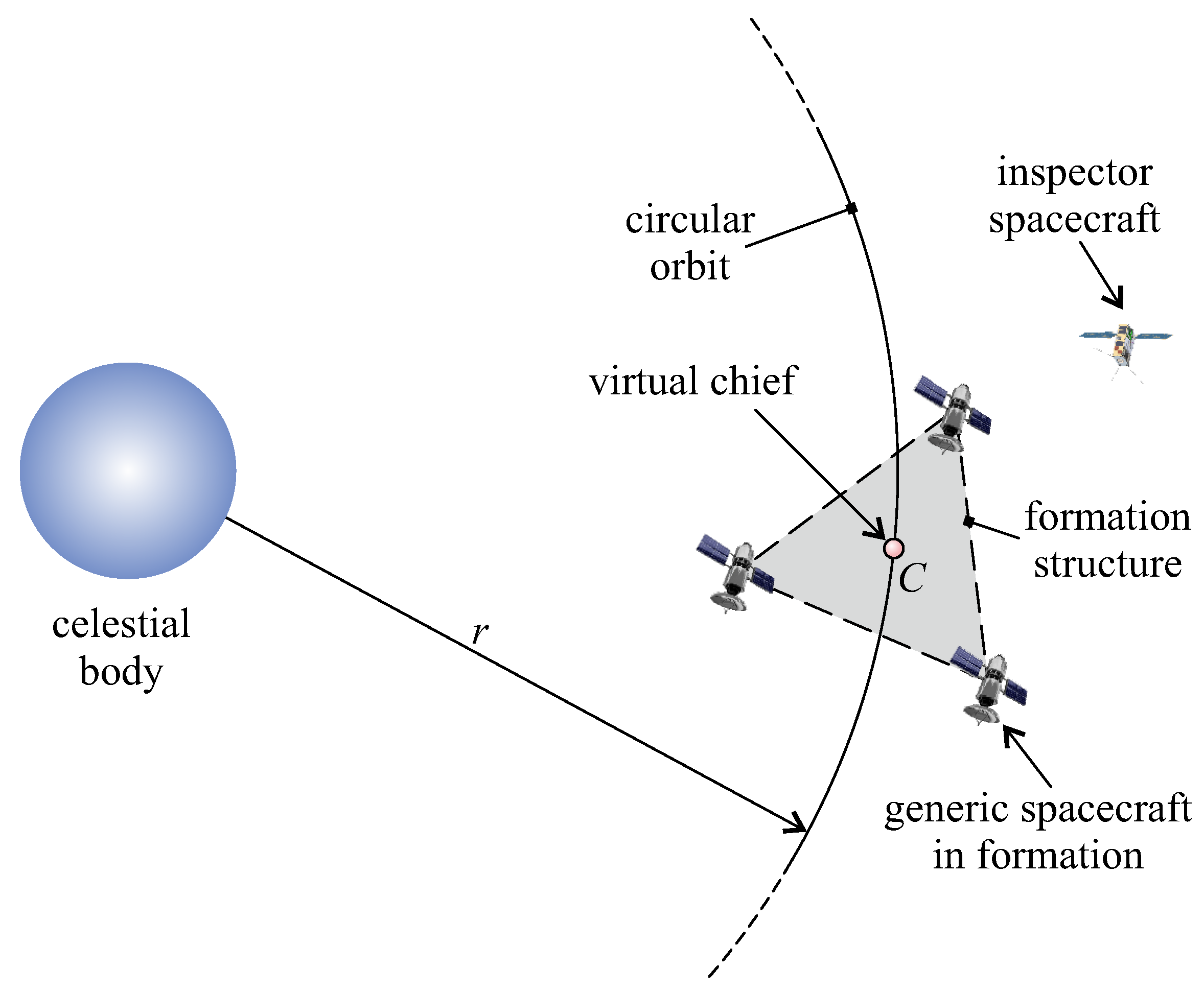
2. Mission Description and Mathematical Model

Consider a formation composed of n 2 satellites flying around a celestial body of gravitational parameter μ . The formation has a virtually rigid structure (with a three-dimensional shape), while virtual chief C traces a Keplerian circular orbit of radius r and prescribed orientation (equivalently, specific angular momentum vector h is assigned). Assume that, when t < t 0 0 , the position of the IS coincides with that of virtual chief C, while its velocity relative to the i-th spacecraft (with i { 1 , 2 , , n } ) in the formation is zero. In other terms, when t < t 0 , the IS and all the satellites in the formation have a constant relative distance and an orbital speed approximately coincident with the speed of virtual chief C along the circular design orbit. The inspection mission starts at time t = t 0 with an impulsive maneuver that inserts the IS into a path that allows for the first inspected satellite to be reached at time t = t 1 > t 0 . Then, a second velocity variation is applied at time t 1 to insert the IS into a second arc that allows for the second spacecraft to be inspected at time t = t 2 > t 1 , as illustrated in Figure 2.
The whole inspection trajectory tracked by the IS can, therefore, be ideally partitioned into a sequence of n Keplerian arcs patched by n 1 impulsive maneuvers. The generic i-th arc starts at time t i 1 , just after the ( i 1 ) -th impulsive maneuver that gives a velocity variation Δ v i 1 , and ends at time t i , just before the i-th impulsive maneuver that gives a velocity variation Δ v i . The IS traces a multiple-impulse rest-to-rest (relative) trajectory; that is, the IS velocity relative to the formation structure is zero at both the beginning (when the IS position coincides with that of C) and the end (when the IS is close to the last inspected spacecraft) of the mission; see Figure 2.
Since the first (or last) arc starts (or ends) with an impulsive velocity variation applied at time t = t 0 (or t = t n ), the total number of required impulsive maneuvers is n + 1 , while the total flight time required by the IS to complete the mission (i.e., to inspect all of the formation spacecraft) is Δ t = t n t 0 t n . The geometry of the generic arc can be obtained by analyzing the IS dynamics relative to the formation, as discussed in the next section.

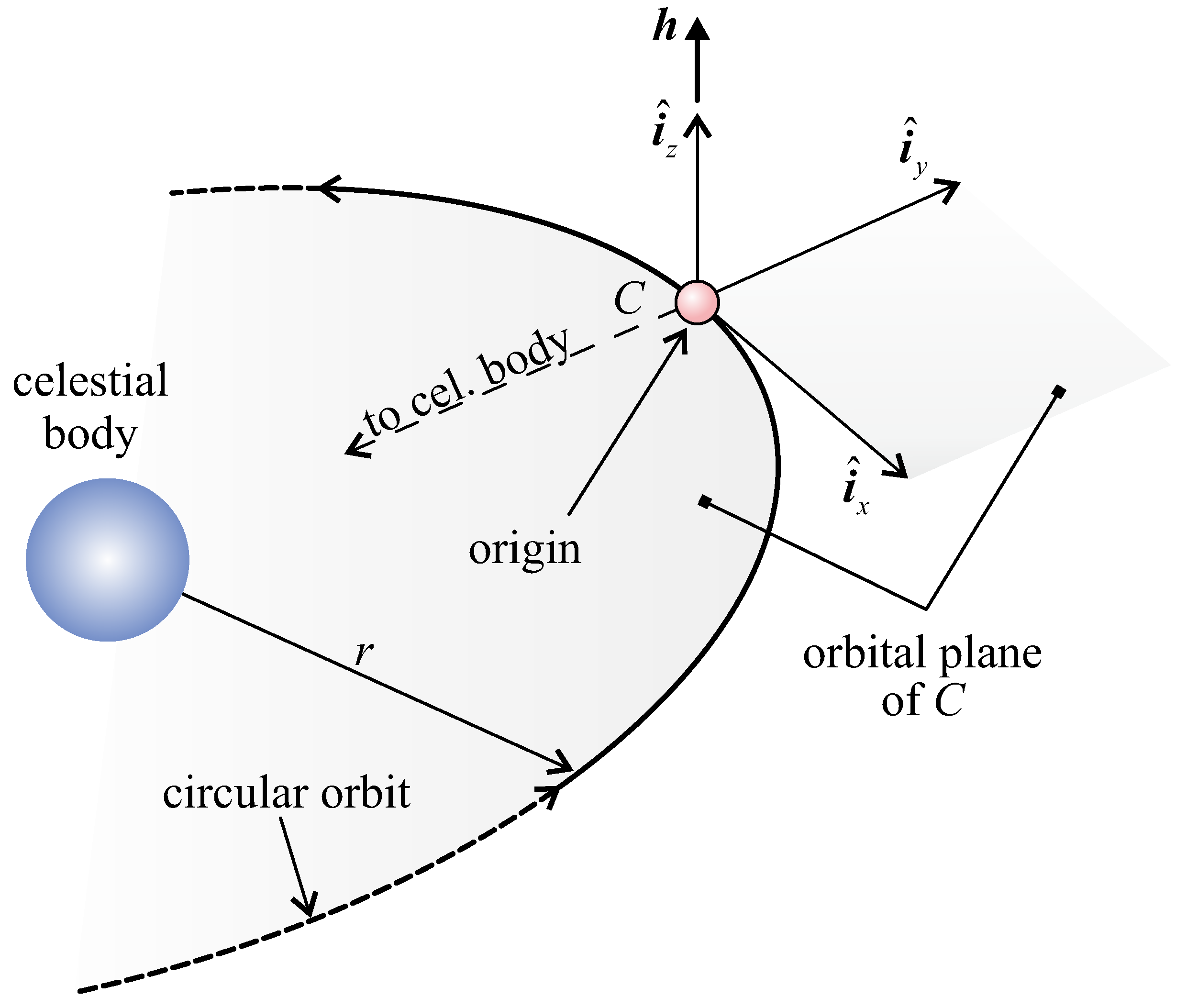
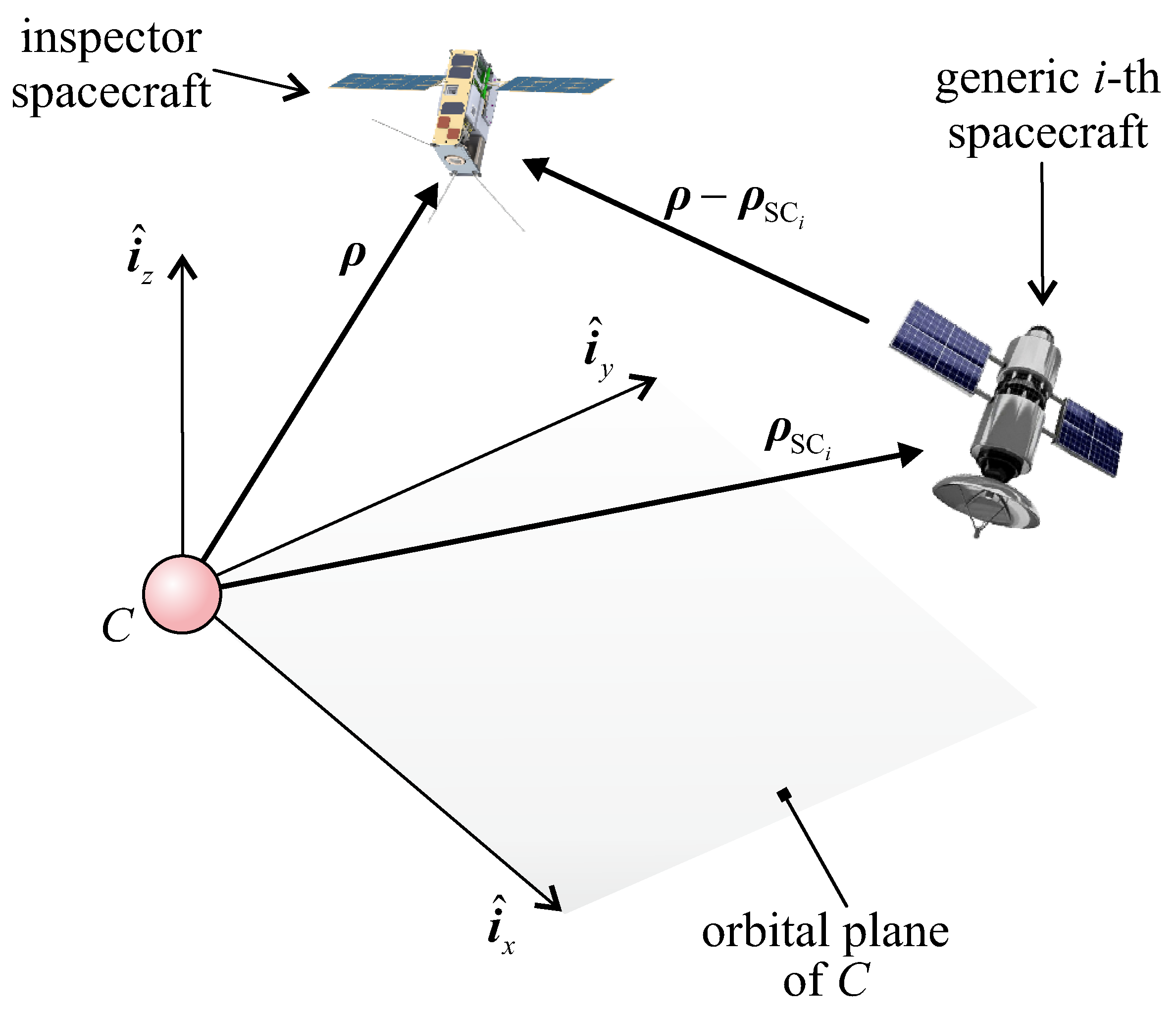
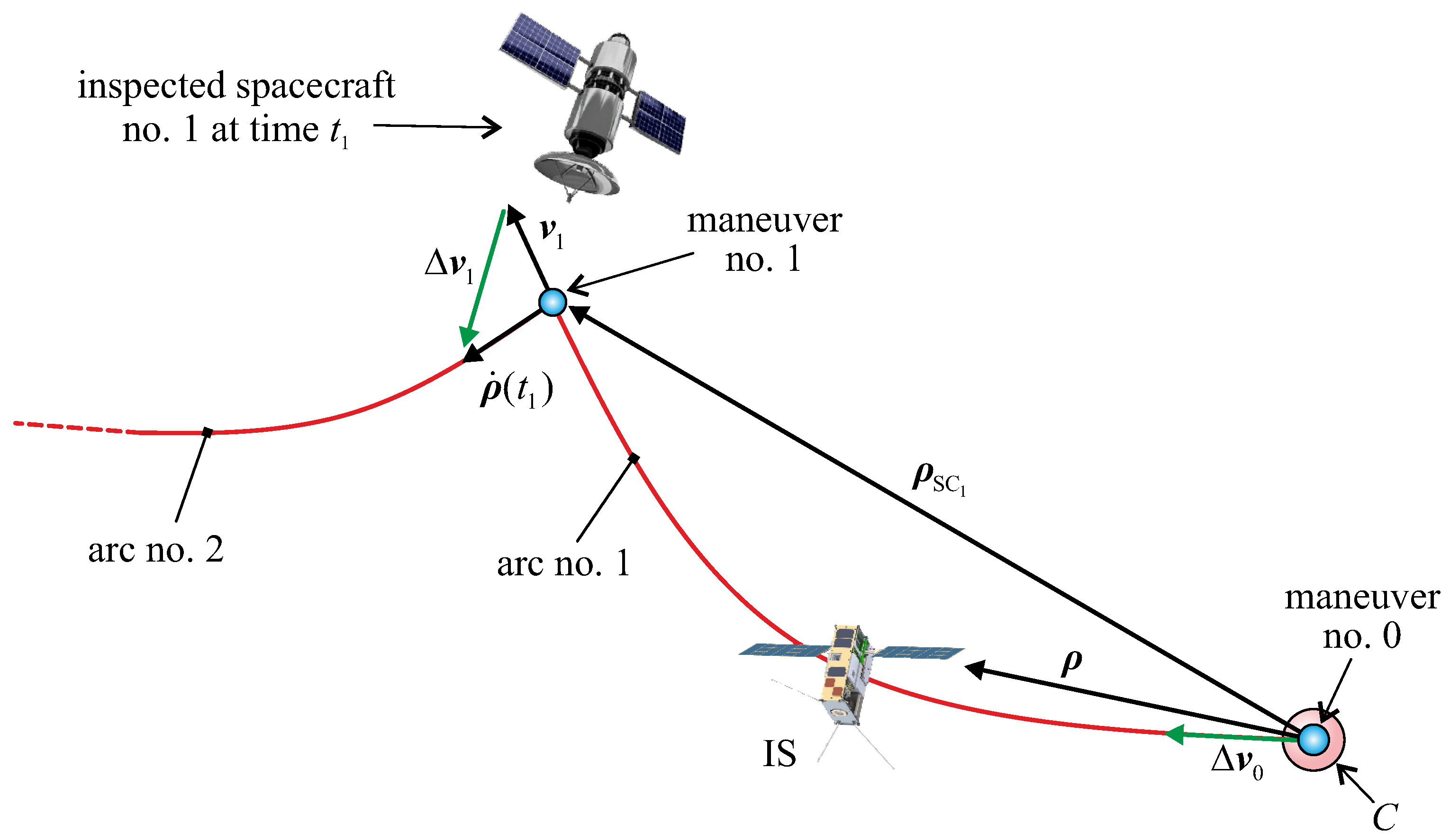
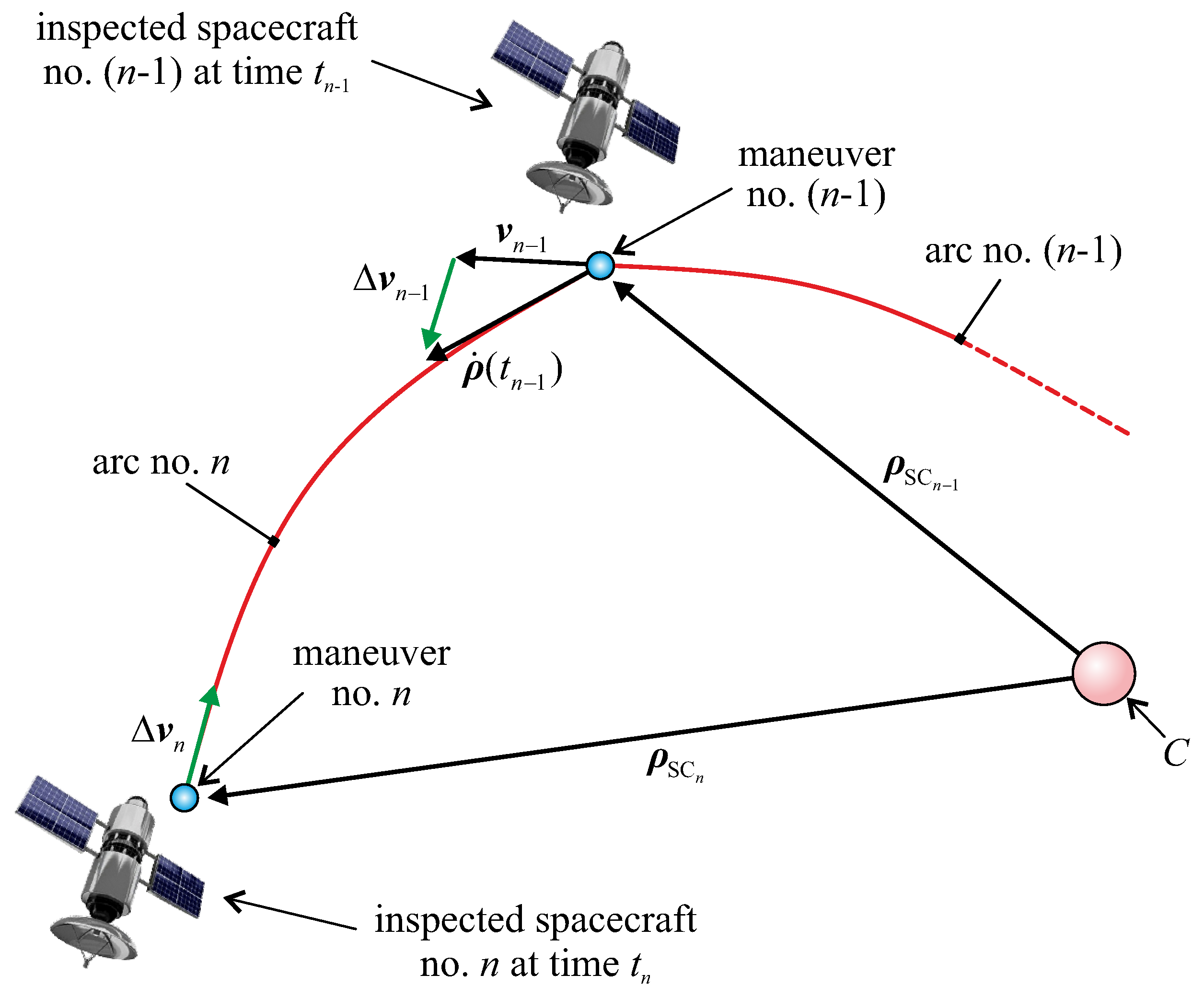
2.1. IS Relative Dynamics

Consider the generic i-th arc, which starts (or ends) at time t i 1 (or t i ). In that arc, the IS dynamics relative to the formation may be described by introducing a local–vertical–local–horizontal (or Hill’s) reference frame T H ( C ; i ^ x , i ^ y , i ^ z ) of origin C in which unit vector i ^ y is aligned with the celestial body-C line, the plane ( i ^ x , i ^ y ) coincides with the orbital plane of virtual chief C, and unit vector i ^ z is aligned with h ; see Figure 3. i ^ x is opposite to the motion direction of C along its circular orbit, while frame T H rotates around the (inertially fixed) direction of h with a period equal to 2 π r 3 / μ .
In the rotating reference frame, the position vector of IS and that of the i-th spacecraft in the formation are denoted by ρ R 3 × 1 and ρ SC i R 3 × 1 , respectively, as illustrated in Figure 4.
The IS motion in T H is described in linearized form by the classical Hill–Clohessy–Wiltshire (HCW) equations [13]:
x ¨ = 2 ω y ˙
y ¨ = 2 ω x ˙ + 3 ω 2 y
z ¨ = ω 2 z
where the dot represents a time derivative, ω μ / r 3 is the constant angular velocity of virtual chief C along the design circular orbit, and { x , y , z } are the three components in the T H of IS position vector ρ . Equations (1)–(3) can be equivalently written as follows.
ρ ¨ + A ρ ˙ + B ρ = 0
where A R 3 × 3 and B R 3 × 3 are two constant matrices defined as
A 0 2 ω 0 2 ω 0 0 0 0 0
B 0 0 0 0 3 ω 2 0 0 0 ω 2
The initial conditions that complete second-order vectorial differential Equation (4) were obtained by enforcing the IS position ( ρ i 1 ) and velocity ( ρ ˙ i 1 ) vectors at the beginning of the i-th arc, that is, just after the ( i 1 ) -th impulsive maneuver. At the beginning of the i-th arc (with i 1 ) the IS is close to the ( i 1 ) -th inspected spacecraft, i.e., the spacecraft with position vector ρ SC i 1 . At time t 0 , when the IS is at C (origin of T H ) with zero velocity relative to the spacecraft in the formation, the initial conditions of Equation (4) in a generic arc can be written as follows.
ρ ( t i 1 ) = 0 if i = 1 ρ SC i 1 if i 1
ρ ˙ ( t i 1 ) = Δ v 0 if i = 1 v i 1 + Δ v i 1 if i 1
where v i 1 is the IS relative velocity vector at the end of the ( i 1 ) -th arc (with i 1 ), that is, just before the ( i 1 ) -th impulsive maneuver that gives velocity variation Δ v i 1 . v i 1 coincides with the value of velocity vector ρ ˙ calculated at the end of the ( i 1 ) -th arc (with i 1 ).
Differential Equation (4) may be solved with standard methods to obtain the time variation in the IS relative position ( ρ ) and velocity ( ρ ˙ ) along the generic i-th arc. Paralleling the procedure detailed in Chobotov’s textbook [13] and observing that, in the i-th arc, the time ranges within interval t [ t i 1 , t i ] , the result is as follows.
ρ ( t ) = M ( t ) ρ ( t i 1 ) + N ( t ) ρ ˙ ( t i 1 )
ρ ˙ ( t ) = S ( t ) ρ ( t i 1 ) + T ( t ) ρ ˙ ( t i 1 )
where { M , N , S , T } R 3 × 3 are time-variant matrices defined as follows.
M ( t ) 1 6 ω t sin ( ω t ) 0 0 4 3 cos ( ω t ) 0 0 0 cos ( ω t )
N ( t ) 1 ω 4 sin ( ω t ) 3 ω t 2 1 cos ( ω t ) 0 2 1 cos ( ω t ) sin ( ω t ) 0 0 0 sin ( ω t )
S ( t ) ω 0 6 1 cos ( ω t ) 0 0 3 sin ( ω t ) 0 0 0 sin ( ω t )
T ( t ) 4 cos ( ω t ) 3 2 sin ( ω t ) 0 2 sin ( ω t ) cos ( ω t ) 0 0 0 cos ( ω t )
Equations (9)–(14) are used to calculate the total velocity variation Δ v tot required by the IS to complete its inspection mission, as discussed in the next section.
The described approach may be extended to the case in which virtual chief C covers an elliptical orbit using the results of Yamanaka and Ankersen [14], who provided a state transition matrix to compute the state of the chaser spacecraft relative to the target at a generic time as a function of the initial state. In that case, Equations (9)–(10) should be properly modified in order for the general case of elliptical orbits to be investigated. However, this issue goes beyond the scope of this paper and is left to future investigations.

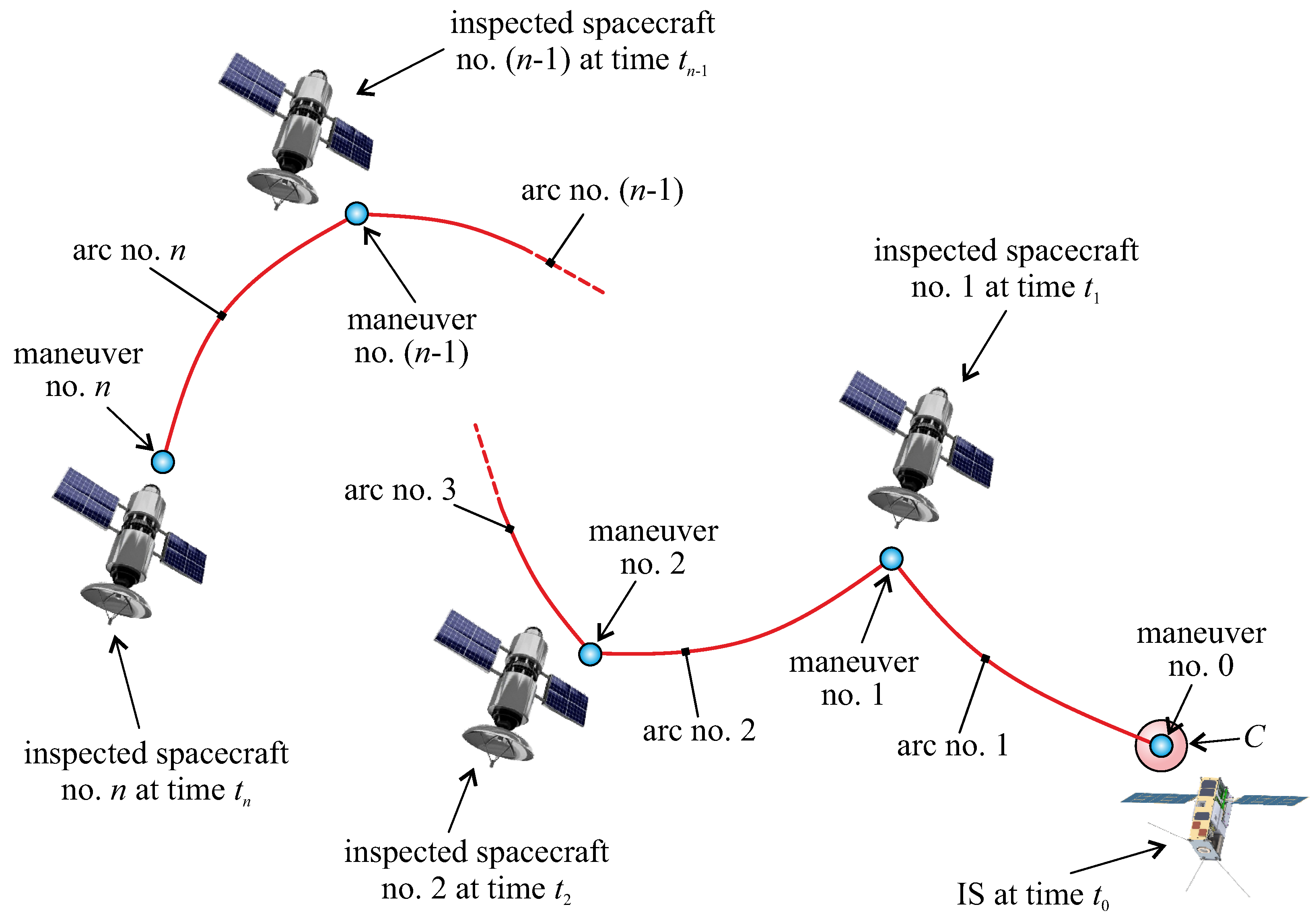
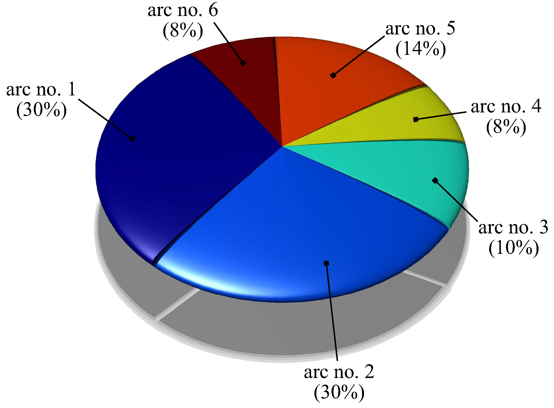
2.2. Total Velocity Variation Evaluation

Total velocity variation Δ v tot is the sum of the magnitude of each (vectorial) velocity variation Δ v that enters Equation (8), that is,
Δ v tot = j = 0 n Δ v j
The components of generic Δ v j , with j { 0 , 1 , , n } , can be recursively calculated as a function of the sequence of inspected spacecraft and of the time instants at which impulsive maneuvers are performed.
For example, consider the first arc, and assume selecting time instant t 1 and the first formation element to be inspected, that is, the components in T H of vector ρ SC 1 ; see Figure 5. t 1 and the first inspected spacecraft are both outputs of the optimization problem described in the next section.
Taking the initial conditions of Equations (7) and (8) into account, and assuming that matrix N ( t 1 ) in Equation (12) is nonsingular, Equation (9) gives the expression of initial velocity variation vector
Δ v 0 = N ( t 1 ) 1 ρ SC 1
The value of Δ v 0 is used to obtain velocity variation vector Δ v 1 just before the beginning of the second arc ( i = 2 ) as a function of time instant t 2 and the position of the second inspected spacecraft, that is, the components in T H of vector ρ SC 2 . In this case, since the IS position at the beginning of the second arc coincides with vector ρ SC 1 , Equations (7)–(9) give
Δ v 1 = N ( t 2 ) 1 ρ SC 2 M ( t 2 ) ρ SC 1 v 1
where v 1 is the (relative) velocity vector ρ ˙ calculated at the end of the first arc through Equation (10):
v 1 = T ( t 1 ) Δ v 0 T ( t 1 ) N ( t 1 ) 1 ρ SC 1 ;
see also Equation (16).
The result from Equation (17) can then be used to evaluate the velocity variation at the end of the third arc, that is, Δ v 2 , as a function of the two additional parameters t 3 and ρ SC 3 . The procedure is then repeated until the IS completes the inspection of the formation structure. The last arc ends with an impulsive maneuver characterized by a velocity variation Δ v n , which stops the IS motion relative to the formation; see Figure 6. The last velocity variation is, therefore, Δ v n = ρ ˙ ( t n ) , so that Equation (10) gives
Δ v n = S ( t n ) ρ SC n 1 T ( t n ) v n 1 + Δ v n 1
where v n 1 is calculated at the end of the last but one or ( n 1 ) -th arc; see Figure 6.
The total velocity variation of Equation (15) is, therefore, a function of 2 n control variables, that is, the sequence of inspected spacecraft (n contributions) and time instants { t 1 , t 2 , , t n } . The control variables can be collected in a control vector u R 2 n × 1 , so that the total velocity variation can be written in a functional form:
Δ v tot = Δ v tot ( u )
n components of the control vector are positive integers that describe the sequence of the inspected formation elements, while the remaining n components are positive real numbers that coincide with the time instants at which the formation satellites are reached, and the impulsive maneuvers are performed. The control vector and total velocity variation are the solution of the optimization problem described in the next section.

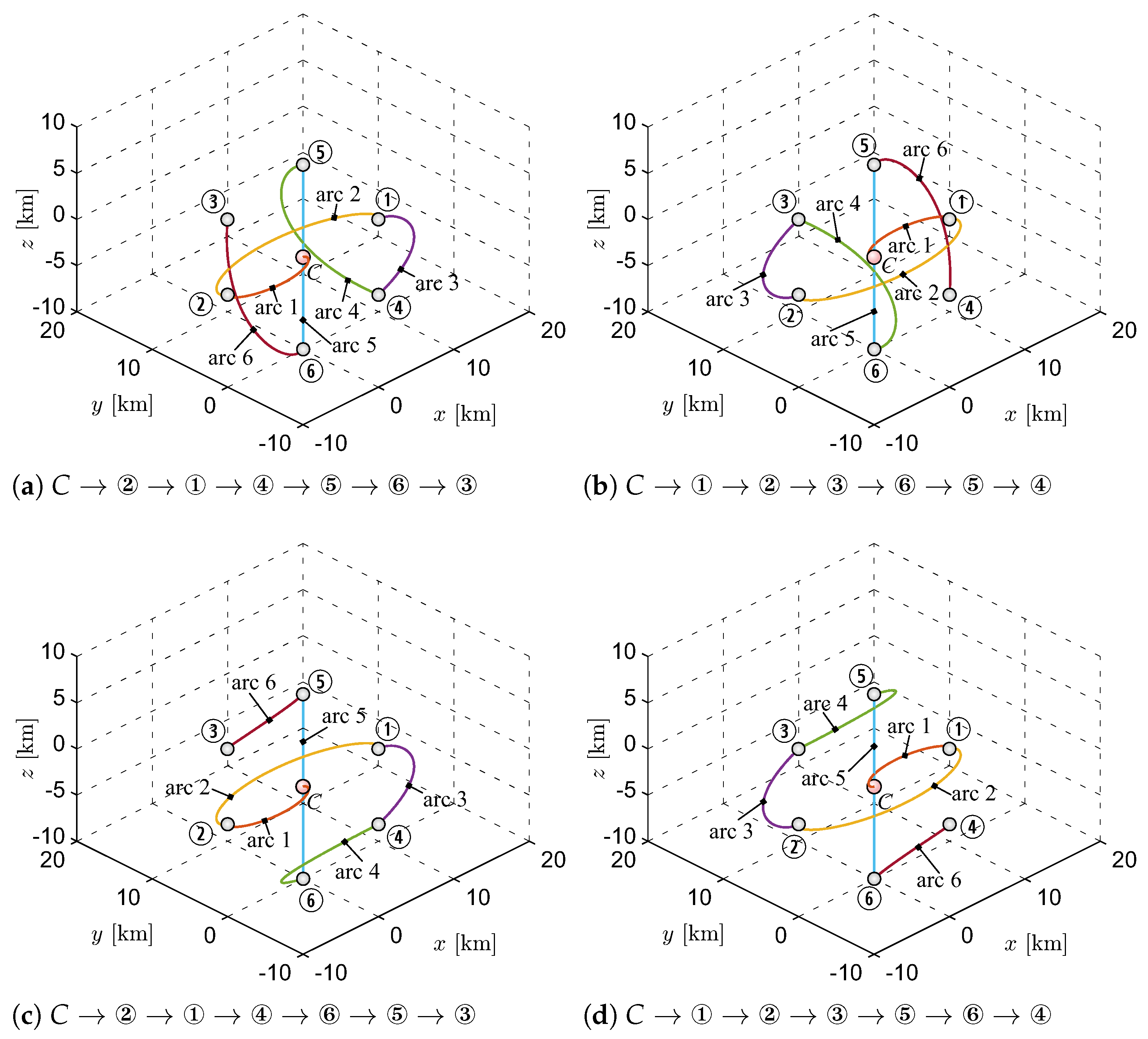
3. Trajectory Optimization and Numerical Simulations

The IS relative trajectory is obtained by evaluating the optimal value of control vector u that minimizes the total velocity variation defined in Equation (20), which coincides with the performance index J of the optimization problem:
J Δ v tot ( u )
The mixed-type components of u (partly constituted by real numbers and partly by integer numbers), which induce J to be characterized by several local minima [15], suggest solving the optimization problem with evolutionary or stochastic algorithms [16] to improve the convergence rate. Paralleling the procedure detailed in [9], on the basis of the evaluation of the success rate parameter introduced by Vasile et al. [17], comparative analysis between some evolutionary and stochastic techniques (including genetic algorithms and particle swarm optimization-based procedures) indicates that a hybrid method that combines differential evolution (DE) algorithms [18,19] and the Nelder–Mead simplex algorithm [20] allows for the optimal value of performance index J to be calculated with reduced computational cost. In particular, the success rate parameter [17] used in the preliminary analysis [9] of the optimization problem is defined as the ratio of the number of times the solution obtained in a test case is close to the optimal value of the performance index J to the total number of algorithm executions.

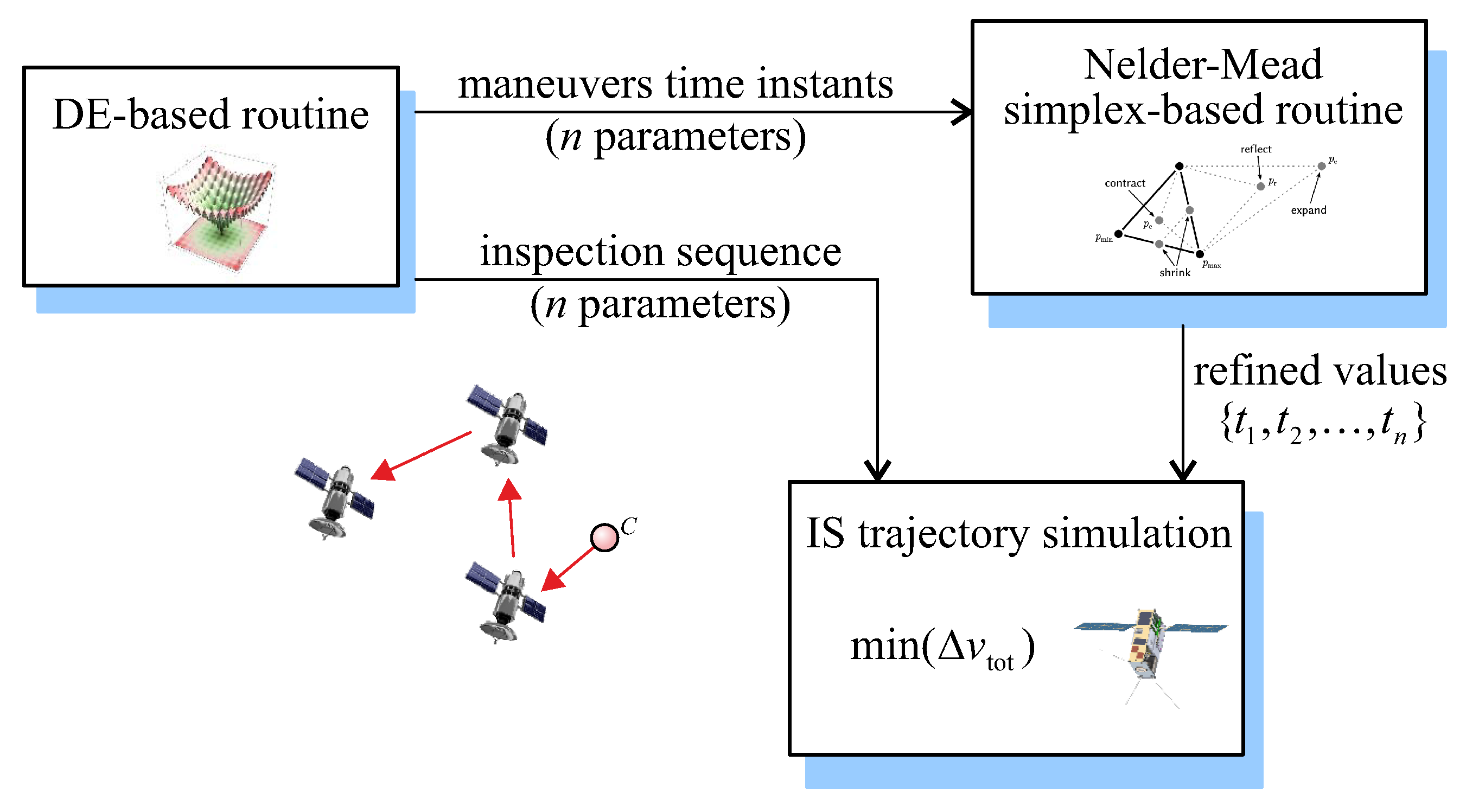
3.1. Two-Step Optimization Procedure

In the proposed two-step procedure, a DE-based method is first used to rapidly obtain an initial guess of the control vector u that allows for the actual minimal value of the total velocity variation to be roughly estimated. Then, the n components of u that define the optimal sequence of inspected formation elements is maintained constant, while the other n components that give maneuver time instants { t 1 , t 2 , , t n } are further refined through a Nelder–Mead simplex-based optimization algorithm, as illustrated in Figure 7.
Such a two-step optimization procedure is an extension of the method used by the authors to solve the two-point boundary value problem associated with a calculus of a variation-based optimization procedure in several trajectory-optimization problems for propellantless [21,22] and continuous-thrust spacecraft [23,24,25]. The proposed procedure resembles the method introduced by Englander et al. [26,27], which uses an algorithm comprising two nested loops: the outer loop determines the integer part of the solution vector (in this case, the sequence of inspected spacecraft), while the inner loop computes the optimal set of maneuver times.
The DE part of the optimization procedure, which is based on the model discussed by Storn and Price [18], begins with the definition of a randomly chosen population of 200 feasible control vectors. The algorithm then selects two random vectors, { u b a n d u c } , and adds their weighted difference to a third vector, u a , through an operation called mutation in order to obtain an updated control vector u m :
u m = u a + β u b u c
where β [ 0.2 , 0.8 ] is a dimensionless positive scaling factor. At that point, a crossover operation is performed in which the components of feasible control vector u m are combined (with a probability of 0.8 ) with a fourth vector, called the target vector, to obtain a new trial vector. Lastly, a selection takes place where the target and trial vector fitness values are compared, and the best survives to the next generation. This procedure is repeatedly applied to all of the population members and for a number of generations equal to 500. The set of parameters used for the DE algorithm is the one that maximizes the success rate, that is, the number of times the algorithm is able to find a solution close to the global minimum [9].
The second part of the two-step optimization procedure, which is based on the use of the Nelder–Mead simplex algorithm, uses built-in MATLAB function fminsearch” to refine the value of the set of maneuver times { t 1 , t 2 , , t n } obtained through the DE-based part (the inspection sequence remains unchanged in this part of the procedure). In this case, the maximal number of function evaluation is set to be 1000 (sufficient for the convergence of the simplex method), while the termination tolerance on the function value is set to be 10 6 . The optimization procedure was applied to a test case that had been studied in the literature [9] in order to validate the results, as discussed in the next section.

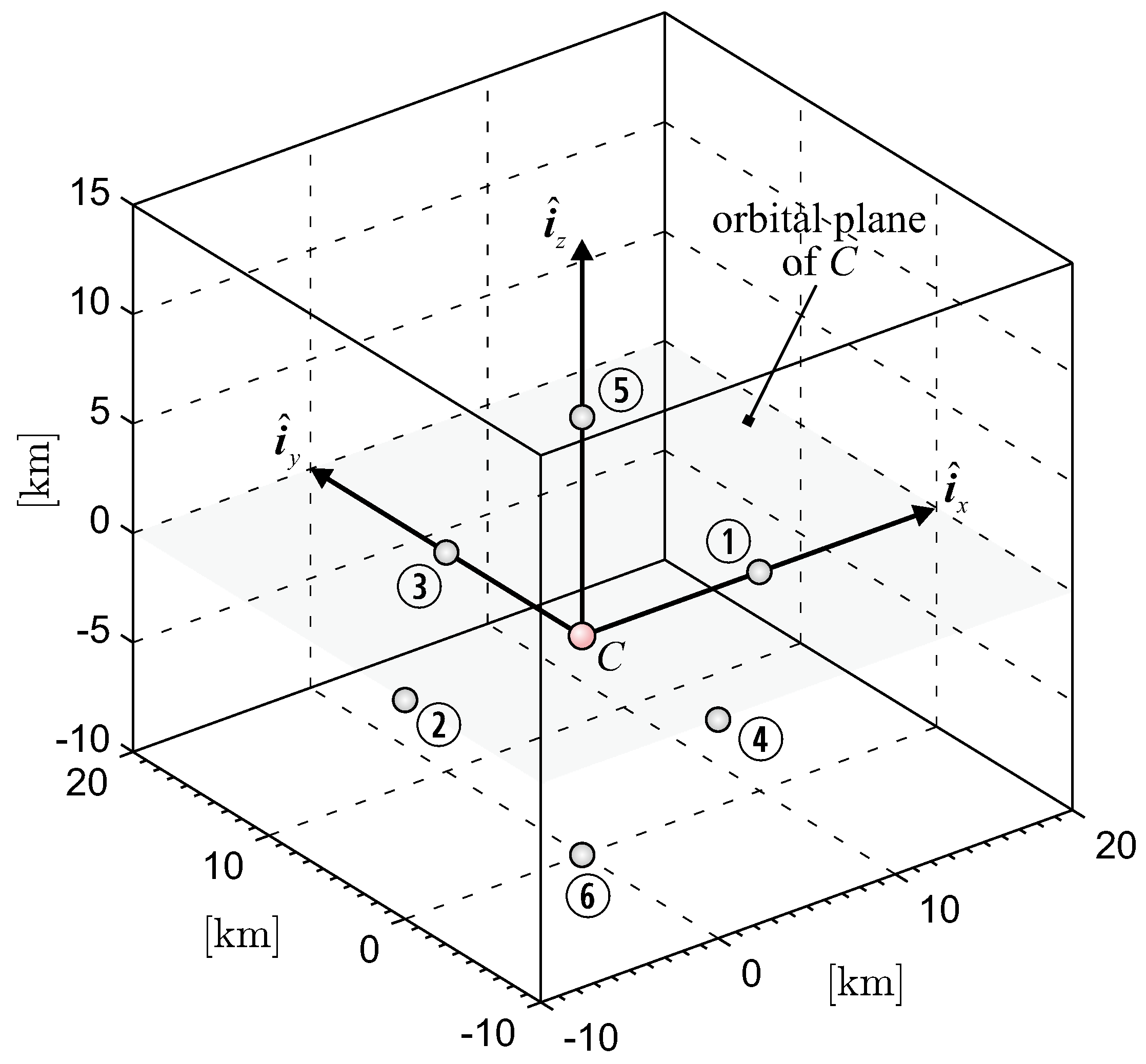
3.2. Test Case and Model Validation

Consider a three-dimensional Earth-centered inspection mission where a formation of n = 6 satellites covers a circular low-Earth orbit of altitude 300 km (Earth’s gravitational parameter is μ = μ 3.986 × 10 5 km 3 / s 2 ). The angular velocity of virtual chief C along the circular orbit is ω 4.164 rad / hour , and the spacecraft formation completes a revolution around the planet in about 90 min .
The components of generic spacecraft position vector ρ SC i are summarized in Table 1, where labels { , , , , , } are used to identify the spacecraft in the formation structure; see also Figure 8. Clearly, the distance between virtual chief C and the generic formation element was much smaller than the distance between the spacecraft and Earth’s center of mass (which is about 6700 km ). Hill–Clohessy–Wiltshire Equations (1)–(3) used in the proposed procedure are, therefore, consistent with the actual dynamics of the IS that, at time t 0 , is at the origin of rotating reference frame T H (point C).
A similar inspection mission scenario was deeply analyzed in [9] by considering a rendezvous with each formation member, and using different optimization algorithms and numerical procedures. The minimal value of the total velocity variation in that case was evaluated by analyzing each of the 720 possible inspection sequences, and optimizing maneuver time instants { t 1 , t 2 , , t n } . The results of [9] gave a minimal value of the total velocity variation of about 91.5 m / s , which is used in this work as a reference (upper) value of performance index J defined in Equation (21).
The procedure proposed in this work gave a minimal total velocity variation of 69.902 m / s , a value consistent with the current technology readiness level (see, for example, the VACCO green propellant integrated propulsion system [28]). In principle, the value of total velocity variation, which was obtained by enforcing a maximal travel time of 2 h along each leg of the IS trajectory, may be reduced by extending the duration of the entire maneuver. However, the computed value of 69.902 m / s was reduced by only a few meters per second when the maximal travel time was increased up to 24 h. To validate our model, the total velocity variation computed with the HCW model was compared with that obtained with a Keplerian motion model. In particular, by solving a series of Lambert’s targeting problems using the optimal sequence of inspected spacecraft and the flight time along each leg computed with the proposed approach, we found a total velocity variation of 69.919 m / s , which is very close to the value obtained with the HCW model. Notably, the optimization of performance index J was obtained with a calculation time that was about one order of magnitude smaller than that required by the method discussed in [9]. The minimal value of velocity variation Δ v tot was reached in four different inspection sequences, as summarized in Table 2, a result that is consistent with the geometric symmetry in the formation structure. The IS inspected trajectories in the four optimal sequences described in Table 2 are shown in Figure 9.
The total flight time, which is an output of the optimization process, was Δ t 5.05 h , while the flight time distribution on the six arcs is reported in the pie chart of Figure 10. The flight time distribution along the six arcs was roughly the same for the four optimal inspection sequences listed in Table 2. This aspect is again consistent with the numerical results of [9].

4. Conclusions

This paper analyzed the optimal rest-to-rest multiple-impulse transfer of an inspector spacecraft in a formation that covers a design circular orbit around an assigned celestial body. Using the linearized Hill–Clohessy–Wiltshire equations, an iterative procedure was detailed to evaluate the total velocity variation required by an inspector spacecraft to carry out a full inspection mission. The minimal value of the total velocity variation was calculated through a two-step procedure that combined DE algorithms and Nelder–Mead simplex method-based routines. The optimization algorithm, which extends and refines a recent technique proposed by the authors in a similar mission scenario, was implemented in such a way that the procedure may handle both real and integer variables. In particular, it is necessary to determine the optimal sequence of inspected spacecraft with the constraint that each spacecraft in the sequence must be unique. Because standard DE algorithms hardly handle this type of constraint, the procedure was slightly modified, so that at each iteration, the algorithm may choose the sequence from a list containing all the spacecraft labels. Once a spacecraft is chosen, it is deleted from the list, so that the subsequent spacecraft can be selected. Moreover, the Nelder–Mead simplex algorithm is only suitable for solving minimization problems of real-valued functions. Therefore, the sequence of inspected spacecraft determined by the DE algorithm is maintained constant during the second step of optimization process, which is a necessary step to refine the solution.
The numerical simulations confirm that the refined procedure allows for computational time to be significantly smaller when compared to that of the previous approach. The natural extension of this work is to analyze a rest-to-rest optimal transfer using a more accurate model of the inspector spacecraft dynamics by including the presence of orbital perturbations, such as the J 2 effect or atmospheric drag. Analysis can also be further extended to the general case where the virtual chief traces an elliptical orbit with the aid of the Tschauner–Hempel equations.

Author Contributions

Conceptualization, A.C. and A.A.Q.; methodology, A.C.; software, A.C.; writing—original draft preparation, A.A.Q., A.C. and G.M.; writing-review and editing, M.B. All authors have read and agreed to the published version of the manuscript.

Funding

This work was partly supported by the University of Pisa, Progetti di Ricerca di Ateneo (grant no. PRA_2022_1).

Data Availability Statement

Not applicable.

Conflicts of Interest

The authors declare no conflict of interest.

References

  1. Alfriend, K.T.; Vadali, S.R.; Gurfil, P.; How, J.P.; Breger, L.S. Spacecraft Formation Flying: Dynamics, Control and Navigation; Butterworth-Heinemann: Oxford, UK, 2010. [Google Scholar] [CrossRef]
  2. Bandyopadhyay, S.; Foust, R.; Subramanian, G.P.; Chung, S.J.; Hadaegh, F.Y. Review of formation flying and constellation missions using nanosatellites. J. Spacecr. Rocket. 2016, 53, 567–578. [Google Scholar] [CrossRef] [Green Version]
  3. Capó-Lugo, P.A.; Bainum, P.M. Orbital Mechanics and Formation Flying: A Digital Control Perspective; Woodhead Publishing: Sawston, UK, 2011. [Google Scholar]
  4. Williams, T. Orbital inspection vehicle trajectories based on line-of-sight maneuvers. Acta Astronaut. 2002, 50, 49–53. [Google Scholar] [CrossRef]
  5. Horri, N.M.; Kristiansen, K.U.; Palmer, P.; Roberts, M. Relative attitude dynamics and control for a satellite inspection mission. Acta Astronaut. 2012, 71, 109–118. [Google Scholar] [CrossRef]
  6. Prince, E.R.; Cobb, R.G. Optimal inspector satellite guidance to quasi-hover via relative teardrop trajectories. Acta Astronaut. 2018, 153, 201–212. [Google Scholar] [CrossRef]
  7. Capolupo, F.; Labourdette, P. Receding-horizon trajectory planning algorithm for passively safe on-orbit inspection missions. J. Guid. Control Dyn. 2019, 42, 1023–1032. [Google Scholar] [CrossRef]
  8. Maestrini, M.; Di Lizia, P. Guidance strategy for autonomous inspection of unknown non-cooperative resident space objects. J. Guid. Control Dyn. 2022, 45, 1126–1136. [Google Scholar] [CrossRef]
  9. Caruso, A.; Mengali, G.; Quarta, A.A. Optimal formation inspection using small spacecraft. In Proceedings of the 4th IAA Conference on University Satellite Missions and CubeSat Workshop, Roma, Italy, 4–7 December 2017. [Google Scholar]
  10. Hill, G.W. Researches in the Lunar Theory. Am. J. Math. 1878, 1, 5. [Google Scholar] [CrossRef]
  11. Alfriend, K.T.; Lee, D.J.; Creamer, N.G. Optimal Servicing of Geosynchronous Satellites. J. Guid. Control Dyn. 2006, 29, 203–206. [Google Scholar] [CrossRef]
  12. Zhang, G.; Ye, D. Optimal short-range rendezvous using on-off constant thrust. Aerosp. Sci. Technol. 2017, 69, 209–217. [Google Scholar] [CrossRef]
  13. Chobotov, V.A. (Ed.) Orbital Mechanics; AIAA Education Series; AIAA: Reston, VA, USA, 2002; Chapter 7; pp. 155–159. [Google Scholar] [CrossRef]
  14. Yamanaka, K.; Ankersen, F. New state transition matrix for relative motion on an arbitrary elliptical orbit. J. Guid. Control Dyn. 2002, 25, 60–66. [Google Scholar] [CrossRef]
  15. Kim, D.Y.; Woo, B.; Park, S.Y.; Choi, K.H. Hybrid optimization for multiple-impulse reconfiguration trajectories of satellite formation flying. Adv. Space Res. 2009, 44, 1257–1269. [Google Scholar] [CrossRef]
  16. Simon, D. Evolutionary Optimization Algorithms; John Wiley & Sons: Hoboken, NJ, USA, 2013; pp. 305–308. ISBN 978-0-470-93741-9. [Google Scholar]
  17. Vasile, M.; Minisci, E.; Locatelli, M. Analysis of Some Global Optimization Algorithms for Space Trajectory Design. J. Spacecr. Rocket. 2010, 47, 334–344. [Google Scholar] [CrossRef] [Green Version]
  18. Storn, R.; Price, K. A Simple and Efficient Heuristic for global Optimization over Continuous Spaces. J. Glob. Optim. 1997, 11, 341–359. [Google Scholar] [CrossRef]
  19. Nocedal, J.; Wright, S.J. Numerical Optimization; Springer: New York, NY, USA, 2006. [Google Scholar] [CrossRef] [Green Version]
  20. Lagarias, J.C.; Reeds, J.A.; Wright, M.H.; Wright, P.E. Convergence properties of the Nelder-Mead simplex method in low dimensions. SIAM J. Optim. 1998, 9, 112–147. [Google Scholar] [CrossRef] [Green Version]
  21. Mengali, G.; Quarta, A.A. Trajectory analysis and optimization of Hesperides mission. Universe 2022, 8, 364. [Google Scholar] [CrossRef]
  22. Bassetto, M.; Caruso, A.; Quarta, A.A.; Mengali, G. Optimal heliocentric transfers of a Sun-facing heliogyro. Aerosp. Sci. Technol. 2021, 119, 1–14. [Google Scholar] [CrossRef]
  23. Mengali, G.; Quarta, A.A. Fuel-optimal, power-limited rendezvous with variable thruster efficiency. J. Guid. Control Dyn. 2005, 28, 1194–1199. [Google Scholar] [CrossRef]
  24. Quarta, A.A.; Mengali, G. Minimum-Time Space Missions with Solar Electric Propulsion. Aerosp. Sci. Technol. 2011, 15, 381–392. [Google Scholar] [CrossRef]
  25. Bassetto, M.; Niccolai, L.; Boni, L.; Mengali, G.; Quarta, A.A.; Circi, C.; Pizzurro, S.; Pizzarelli, M.; Pellegrini, R.C.; Cavallini, E. Sliding Mode Control for Attitude Maneuvers of Helianthus Solar Sail. Acta Astronaut. 2022, 198, 100–110. [Google Scholar] [CrossRef]
  26. Englander, J.; Conway, B.A.; Williams, T. Automated Interplanetary Trajectory Planning. In Proceedings of the AIAA/AAS Astrodynamics Specialist Conference, Minneapolis, MN, USA, 13–16 August 2012. [Google Scholar] [CrossRef]
  27. Englander, J.A.; Conway, B.A.; Williams, T. Automated Mission Planning via Evolutionary Algorithms. J. Guid. Control Dyn. 2012, 35, 1878–1887. [Google Scholar] [CrossRef]
  28. Cappelletti, C.; Battistini, S.; Malphrus, B.K. CubeSat Handbook. from Mission Design to Operations; Elsevier Science: Amsterdam, The Netherlands, 2020; Chapter 15; pp. 287–294. ISBN 978-0-128-17884-3. [Google Scholar]
Figure 1. Conceptual sketch of a formation with three vehicles and a CubeSat inspector spacecraft.
Remotesensing 14 05192 g001
Figure 2. Scheme of the multiple-impulse, rest-to-rest, IS relative trajectory.
Remotesensing 14 05192 g002
Figure 3. Local–vertical–local–horizontal (or Hill’s) reference frame T H ( C ; i ^ x , i ^ y , i ^ z ) .
Remotesensing 14 05192 g003
Figure 4. Spacecraft position vector in T H .
Remotesensing 14 05192 g004
Figure 5. Impulsive maneuvers at the first and second arcs.
Remotesensing 14 05192 g005
Figure 6. Last two arcs and impulsive maneuvers.
Remotesensing 14 05192 g006
Figure 7. Conceptual sketch of the two-step optimization procedure.
Remotesensing 14 05192 g007
Figure 8. Test case formation structure in rotating reference frame T H .
Remotesensing 14 05192 g008
Figure 9. Optimal IS inspection trajectories in the four optimal sequences listed in Table 2.
Remotesensing 14 05192 g009
Figure 10. Duration of the generic arc in percentages of the total flight time Δ t 5.05 h .
Remotesensing 14 05192 g010
Table 1. Position vector components of the formation elements in the test case inspection scenario.
SC Label ρ SC i · i ^ x [km] ρ SC i · i ^ y [km] ρ SC i · i ^ z [km]
1000
−1000
0100
0−100
0010
00−10
Table 2. Inspection sequences that give a total velocity variation of about 70 m / s .
SequenceSC Label
first C
second C
third C
fourth C
Publisher’s Note: MDPI stays neutral with regard to jurisdictional claims in published maps and institutional affiliations.

