Technical Note

A Novel Dual-Branch Neural Network Model for Flood Monitoring in South Asia Based on CYGNSS Data

1
College of Oceanography and Space Informatics, China University of Petroleum (East China), Qingdao 266580, China
2
Laboratory for Marine Mineral Resources, Qingdao National Laboratory for Marine Science and Technology, Qingdao 266071, China
3
National Space Science Center, Chinese Academy of Sciences, Beijing 100190, China
*
Author to whom correspondence should be addressed.
Remote Sens. 2022, 14(20), 5129; https://doi.org/10.3390/rs14205129
Submission received: 13 August 2022 / Revised: 8 October 2022 / Accepted: 10 October 2022 / Published: 14 October 2022
(This article belongs to the Special Issue GNSS-R Earth Remote Sensing from SmallSats)

Abstract

:
Microwave remote sensing is widely applied in flood monitoring due to its independence from severe weather conditions, which usually restrict the usage of optical sensors. However, it is challenging to track the variation process of flood events in a timely manner by traditional active and passive microwave techniques, since they cannot simultaneously provide measurements with high spatial and temporal resolution. The emerging Global Navigation Satellite System Reflectometry (GNSS-R) technique with high spatio-temporal resolution offers a new solution to the dynamic monitoring of flood inundation. Considering the high sensitivity of GNSS-R signals to flooding, this paper proposes a dual-branch neural network (DBNN) with a convolution neural network (CNN) and a back propagation (BP) neural network for flood monitoring. The CNN module is used to automatically extract the abstract features from delay-Doppler maps (DDMs), while the BP module is fed with GNSS-R typical features, such as surface reflectivity and power ratio, as well as vegetation information from Soil Moisture Active Passive satellite (SMAP) data. In the experiments, the superiority of the DBNN method is firstly demonstrated by comparing it with the surface reflectivity and power ratio methods. Then, the spatio-temporal variation process of the 2020 South Asian flood events is analyzed by the proposed method based on Cyclone Global Navigation Satellite System (CYGNSS) data. The understanding of flood change processes could help enhance the capacity for resisting flood disasters.

Graphical Abstract

1. Introduction

The arrival of South Asia’s annual southwest monsoons usually brings continuous heavy rainfall, leading to significant flood events and other natural disasters in parts of India, Nepal, and Bangladesh. The particularly noticeable flood inundation event in 2020 was South Asia’s most significant flood disaster over the past decade, causing huge property losses to local people [1,2,3]. Due to the highly dynamic nature of floods, rapid and effective flood monitoring is important for early disaster prevention, midterm relief, and post-disaster reconstruction [4].
The existing remote sensing means for flood monitoring mainly include optical and microwave remote sensing. However, optical remote sensing means cannot be used on rainy and cloudy days due to the sensors’ inherent characteristics, although they are capable of obtaining Earth surface observations with a satisfactory spatial resolution [4,5,6,7]. Conversely, passive microwave sensors, such as radiometers, have the ability to penetrate clouds and heavy fog owing to their long wavelength, which is requisite for flood monitoring as floods often occur during the rainy season. Nevertheless, the low spatial resolution of even dozens of kilometers limits the successful applications of passive microwave sensors for flood monitoring. On the other hand, active microwave remote sensing normally has a higher spatial resolution than passive microwave remote sensing. However, it also has a relatively lower temporal resolution and is still unable to conduct dynamic flood monitoring in a timely manner [
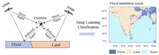
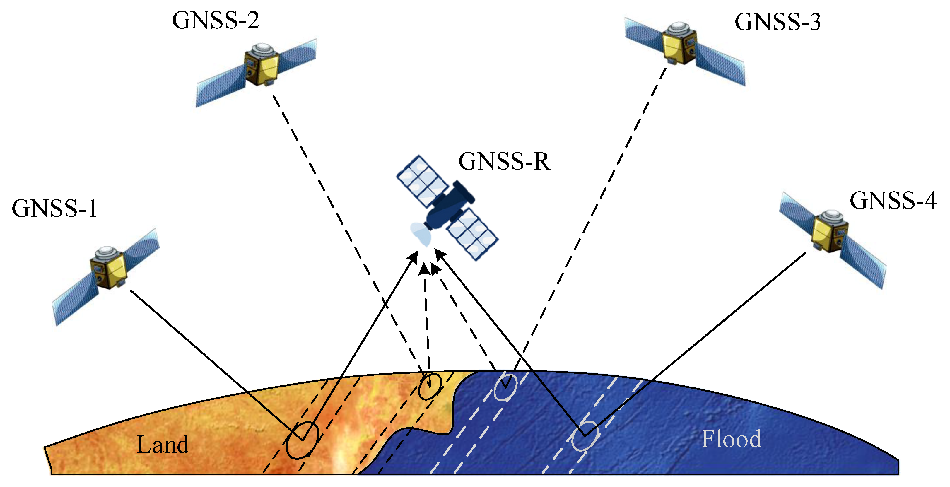
8]. The recently developed Global Navigation Satellite System Reflectometry (GNSS-R) is a novel remote sensing technology for physical parameter inversion by means of GNSS signals reflected from the Earth’s surface [9,10,11]. The Cyclone Global Navigation Satellite System (CYGNSS), launched by NASA, provides openly accessed GNSS-R data, which has been successfully employed in the inversion of sea surface wind speed [12,13,14], soil moisture estimation [15,16,17], flood dynamics monitoring [7,18,19], and other features. The CYGNSS constellation constitutes eight small satellites, on which the receivers are mounted to capture the direct and reflected signals from the navigation satellites. The average revisit period of CYGNSS is only 7 hours, and the spatial resolution is about 3.5 km × 0.5 km on the land surface. Compared with other microwave remote sensing technologies, CYGNSS simultaneously provides observations with higher spatio-temporal resolution, which can be more suitable for dynamic flood monitoring [18,20,21].
Research on GNSS-R flood monitoring first began in 2018. Chew produced a flood inundation map using surface reflectivity (SR) on specular points [18]. Based on CYGNSS data, Wei Wan and Wentao Yang also conducted flood monitoring by surface reflectivity in 2019 and 2021, respectively [7,19]. Furthermore, Unnithan produced large-scale, high-resolution flood inundation maps in 2020 by combining the feature of signal-to-noise ratio in delay-Doppler maps (DDMs) with the topographic information [22]. Through further research, Chew proposed a theoretical model for flood monitoring based on changes in surface reflectivity in different land cover types in 2020. The research results showed that surface reflectivity was mainly dependent on surface roughness. When flood events occurred, the surface reflectivity in densely vegetated areas greatly varied, while that of the relatively smooth surfaces changed little, both before and after the flood [20]. Later, Al-Khaldi proposed the power ratio (PR) method in 2021 to detect water bodies using the coherent properties of DDMs from CYGNSS, and found that over 90% of the land surface reflections presented incoherent scattering, while about 80% of the coherent reflections were related to water bodies [23].
Reviewing the current GNSS-R flood monitoring methods, it is found that most of them are only based on a specific GNSS-R physical feature, such as SR, PR, or signal-to-noise ratio. However, one single GNSS-R feature cannot simultaneously represent the dielectric constant and roughness of the reflective surface. For example, SR is calculated from the power of the specular point [7], so it mainly represents the dielectric property of the specular point rather than the roughness property of the reflective surface, which is essential for the flood inversion [24]. Furthermore, the impact of vegetation on GNSS (direct and reflected) signals has not yet been considered in the available literature [24,25]. As the primary observation data of GNSS-R, DDMs contain much useful detailed information, such as SR and PR. Some scholars have utilized DDMs-based features for flood monitoring, such as PR and signal-to-noise ratio. However, the valuable information in DDMs has not yet been fully excavated. In recent years, deep learning (DL) has been widely employed to automatically learn feature representations from data and establish the intrinsic relationship between inputs and outputs [26]. Among a variety of DL algorithms, convolution neural network (CNN) has surpassed most other DL algorithms in two-dimensional image processing due to its local connectivity, weight sharing, and down-sampling strategies, which can reduce the complexity of neural networks and successfully learn feature representations of images [26]. Moreover, the back propagation (BP) neural networks have powerful nonlinear mapping ability, which is especially suitable for solving the complicated internal mapping problem between one-dimensional input vectors and outputs [
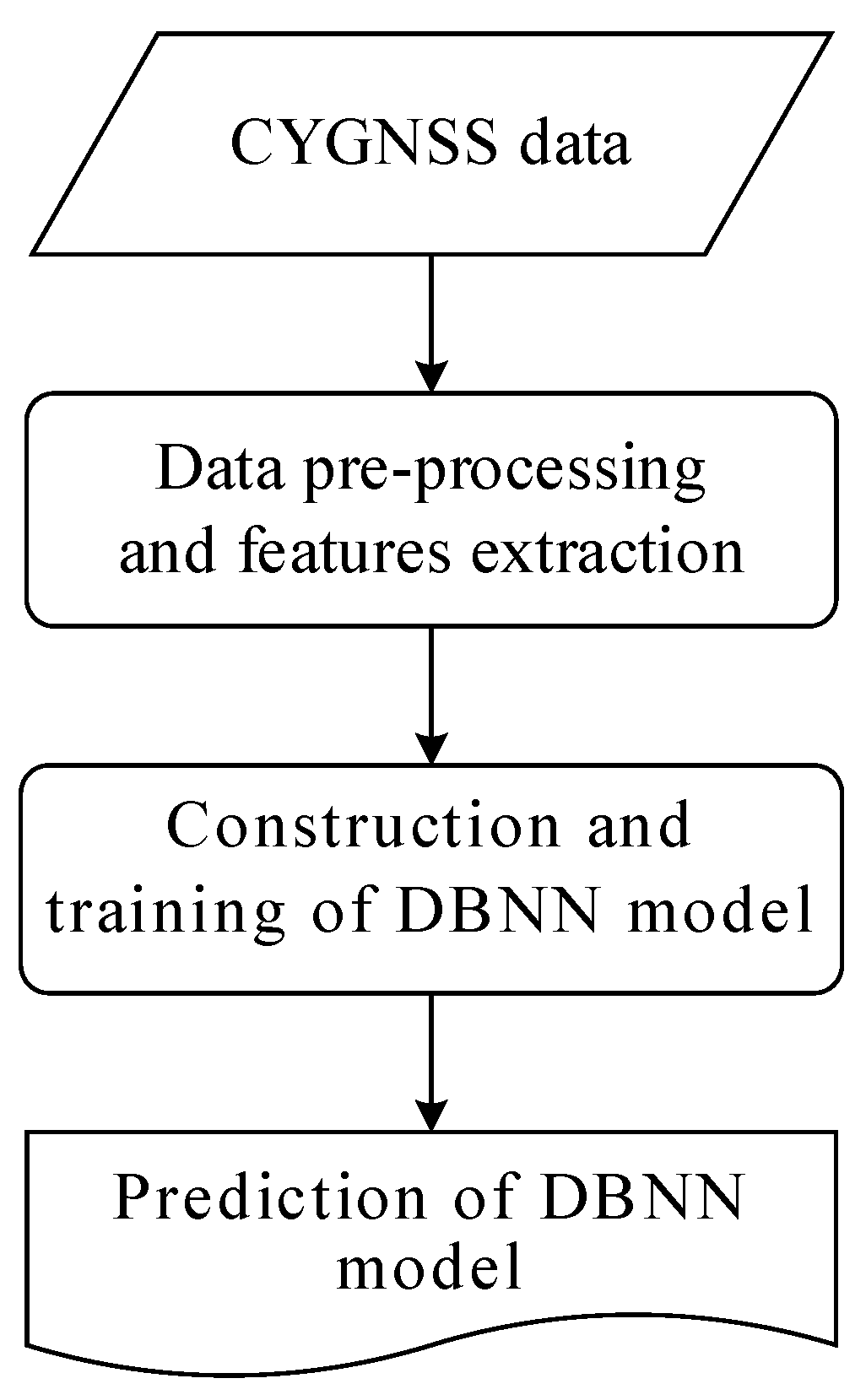
27]. Therefore, by combining a CNN and a BP neural network in parallel, a dual-branch neural network (DBNN) is constructed for better flood monitoring. In the model, the CNN takes two-dimensional DDMs as input and automatically extracts the deep abstract features in DDMs. The BP neural network is fed with the existing typical GNSS-R features and the vegetation information provided by the Soil Moisture Active Passive satellite (SMAP) [28].
The rest of this paper is organized as follows. Section 2 provides the descriptions of CYGNSS data, SMAP data, and the study area. Section 3 introduces the proposed method in detail. The experimental results and discussion are given in Section 4. Finally, Section 5 concludes the study.

2. Data and Study Area

2.1. CYGNSS Data

The GNSS-R data in this study were produced from the CYGNSS constellation, a bi-static radar system (shown in Figure 1). This constellation is capable of collecting the near-global (between 38°N and 38°S latitudes) daily reflected L-1 coarse acquisition GPS signals in the form of DDMs [29,30,31,32]. CYGNSS data have been widely employed in GNSS-R scientific research and other practical applications [30]. The mean and median revisit periods of the CYGNSS were 7 h and 3 h, respectively. The spatial resolution is related to surface roughness, which is around 3.5 km × 0.5 km on the land surface and about 25 km × 25 km on the rough sea surface [23]. Compared with conventional microwave remote sensing, the CYGNSS has higher spatial and temporal resolution in observing the Earth’s surface, which is conducive to in-depth scientific research by GNSS-R techniques [21,24,33].
The data employed in this study is the 3.0 version CYGNSS product at L1 level, which primarily contains DDMs and a range of metadata describing the geometry and instrument parameters in acquisition. CYGNSS data can be acquired in NetCDF format from https://podaac.jpl.nasa.gov (accessed on 10 September 2021). The primary variables utilized are summarized in Table 1; including DDMs, the transmitter/receiver distance to the specular point, transmitter and receiver, antenna gain, etc.

2.2. SMAP Data

The SMAP mission, launched by NASA in January 2015, has been designed to collect L-band signals which are sensitive to land surface soil moisture (~5 cm of depth). The SMAP satellite is equipped with active radar and passive radiometer sensors. However, the radar failed to work in orbit after two months. Hence, the satellite currently relies only on the L-band radiometer to retrieve land surface information, such as soil moisture and vegetation information, by measuring brightness temperature. Since the signals received by SMAP satellite and GNSS signals are both L-band with similar frequencies and sensitivity to the land surface, SMAP data can be employed for comparison analysis with CYGNSS data. The SMAP satellite observes land area between 85°S and 85°N, with a revisit frequency of 2–3 days [28].
The data product utilized in this study is the SMAP Enhanced L3 Radiometer Global Daily 9 km EASE-Grid Soil Moisture, available at https://nsidc.org/data/SPL3SMP_E/versions/4 (accessed on 16 October 2021) [34,35,36]. The enhanced SMAP product is an interpolated and gridded result of SMAP Radiometer measurements, which are posted to the 9 km Equal-Area Scalable Earth Grid, Version 2.0 (EASE-Grid 2.0). The primary data are summarized in Table 2. It is worth noting that two datasets from SMAP, soil moisture and vegetation opacity, were employed in this study. Soil moisture is used to verify the accuracy of the inversion results, while vegetation opacity information is fed as auxiliary input data to the model for flood inversion.

2.3. Study Area

South Asia is an ideal area for flood inversion research using GNSS-R technology, due to its frequent large-scale flooding inundation. As shown in Figure 2, the subgraph (a) displays the coverage area of one CYGNSS satellite in a day, and the subgraph (b) represents the intercepted area of South Asia ranging from 4°N–28°N and 66°E–96°E. The northern part of the region is the Himalayan mountains, with an average elevation of more than 6000 meters; the central part is the Great Plain, with dense river networks and numerous irrigation canals; and the southern part is the Deccan Plateau. The total land area of the study area is approximately 3.24 million square kilometers. In addition, the region is situated in a tropical monsoon climate, with the hot season usually from March to May, the rainy season usually from June to October, and the cool season usually from November to the following February. During the rainy season, the southwest monsoons carry large amounts of water vapor as they pass over the warm ocean, leading to extremely abundant rainfall in South Asia. In 2020, the rainy season in South Asia lasted from June to September, causing the region to experience the most severe flooding of the past decade. Therefore, CYGNSS data ranging from May to October 2020 are selected to conduct the flood inversion, as well as the spatio-temporal dynamic analysis by the proposed DBNN model.

3. Method

In this study, a DBNN model for flood monitoring is proposed, which is mainly composed of two parallel subnetworks: the CNN and BP neural network. In this model, two-dimensional DDMs are input into the CNN, which automatically extracts the abstract features from images, while the BP neural network is fed with seven typical GNSS-R features, including surface reflectivity [18], power ratio [23], and the leading edge of slope [37], etc., as well as vegetation information from SMAP data [28]. The output results of the model are the probability values that DDMs belong to the submerged region. The proposed method consists of three steps, as follows: (1) data pre-processing and features extraction; (2) construction and training of DBNN model; and (3) prediction of DBNN model. The process of this method is shown in Figure 3.

3.1. Data Pre-Processing and Features Extraction

In order to obtain good inversion results, only CYGNSS data meeting the following conditions are employed in this study:
(1)
If the SNR of DDM is too small, there are fewer signals and more noise in the DDM. Therefore, the DDMs are filtered out with SNR less than 1.5 dB.
(2)
The left-handed circular polarization signals received by CYGNSS decrease with the increase of the incident angle. When the incident angle is larger than 65°, the proportion of the left-handed circular polarization signals rapidly decreases; thus, DDMs with the incident angle larger than 65° are filtered out in this study [7,38].
(3)
In this study, only DDMs with transmitter and receiver antenna gain greater than 0 are selected according to the references [25,38].
(4)
The positions of the peak points move toward the edge of DDMs with altitude, and the DTU10 digital elevation model used by CYGNSS does not sufficiently consider the effect of land topography, which results in significant errors in the estimation of positions of specular points with elevations greater than 600 m [23]. Thus, in this study, only DDMs with peak points occurring in delay bins inside of 7–10 pixels are retained [38].
The power values of some pixels in DDMs, which cannot be mapped to the real Earth’s surface, are mainly generated by thermal noise (as shown in the white area in Figure 4). Fortunately, the thermal noise pixels in DDMs can be eliminated by using the method provided by Al-Khaldi [23] after screening CYGNSS data. The DDMs before and after removing the thermal noise pixels are displayed in Figure 5.
The dielectric constant and roughness of the land surface obviously vary when floods occur, so they can be regarded as very useful physical parameters for judging whether floods have occurred or not. Therefore, seven features related to the above two parameters are extracted from DDMs in this study as the inputs of the BP neural network, which include surface reflectivity [18], power ratio [32], leading edge of slope [37], trailing edge of slope [25], peak point power, DDM average [39], and signal-to-noise ratio [12] (as shown in Table 3).

3.2. Construction and Training of DBNN Model

3.2.1. Construction of DBNN Model

The DBNN model consists of two parallel sub-networks, the CNN module and the BP neural network module, which are followed by a concatenate layer, a full connection layer, and an output layer, as illustrated in Figure 6b. In this model, the CNN module consists of two convolutional layers, made up of 16 and 32 the 3 × 3 convolution kernels, respectively, and two pooling layers. Each convolution kernel can be regarded as a feature extractor, which convolves with the input DDMs to generate feature maps. Taking the operation of the kth convolution kernel in the first convolution layer as an example, the input DDM is processed by the convolution kernel to generate the feature map h k ( 1 ) , which can be expressed as follows:
h k ( 1 ) = f ( ( W k ( 1 ) X ) + b k ( 1 ) )
where X is the input DDM, W k ( 1 ) and b k ( 1 ) are the weight and bias of the kth convolution kernel respectively, represents the convolution operation, and f denotes the activation function; this study adopts the widely used ReLU function with the following equation:
f ( z ) = max ( 0 , z )
The max pooling layers with size 2 × 2 and stride 2 are applied in the CNN module to downsample the feature maps from the convolution layers, so as to reduce the redundant information and retain critical features.
In the DBNN model, the BP module consists of two fully connected layers equipped with 16 and 32 neurons, respectively. Each neuron in the module conducts the weighted summation operation on the inputs, which is subsequently processed by the ReLU activation function to create an output feature. As an example, consider the operation of the ith neuron in the first fully connected layer, its output feature y i ( 1 ) can be expressed by the following equation:
y i ( 1 ) = f ( ( x j × w i j ( 1 ) ) + b i ( 1 ) )
where x j is the jth input feature of the neuron, w i j ( 1 ) and   b i ( 1 ) are the weight and bias of this neuron, respectively. f ( · ) denotes the ReLU activation function.
The features output from the CNN module and the BP module are then transferred into the concatenation layer. After being further nonlinearly processed by the full connection layer with 64 neurons, these concatenated features are finally delivered to the output layer. The output layer contains two neurons with the softmax activation function [40,41,42] and outputs probabilities p i of the input DDM corresponding to the submerged region and the unsubmerged region, respectively. The probabilities p i can be expressed as follows:
p i = exp ( v i ) j = 1 k exp ( v j )   w h e r e   i = 1 , 2
where k is the number of neurons in the output layer, set to 2; and v 1 , v 2 are the input values of the softmax function. It should be noted that the softmax function in the neural networks outputs a set of probability values belonging to each classification category, and the summation of all probability values equals 1, where the category corresponding to the largest probability value is the attribution category of the sample. As a binary classification model, the proposed DBNN model only outputs two probability values. Therefore, if there is a probability value greater than 0.5, the corresponding category will be identified as the classification category. Since there are only two probability values output from the DBNN model and their summation is 1, the probability value belonging to the flooded region can be selected as the prediction result of the model. Therefore, samples with probability values greater than 0.5 are regarded as submerged.

3.2.2. Training of DBNN Model

The dataset in this study is obtained by spatio-temporal matching of CYGNSS data and SMAP data ranging from May to September 2020, where CYGNSS data provide DDMs and seven features, as shown in Table 3, and SMAP data offer vegetation information and the target label derived from the classification results of inundated versus non-inundated areas classified by SMAP soil moisture [43]. In this study, 50,000 samples were randomly selected from the dataset as the sample set of the DBNN model, and the sample set was divided into training, validation, and testing subsets at a rate of 80%, 15%, and 5%, respectively [15]. These subsets are designed to provide sufficient data to train the network, evaluate its performance, and tune the hyper-parameters. In addition, all the remaining samples in the dataset are predicted by the DBNN model for the inversion of flood monitoring.
The information forward propagation and the error back-propagation algorithms are adopted for the training of the DBNN model. During the forward propagation, the parameters of the neural network are constant, while in the backward propagation, the parameters are automatically updated to minimize the loss function using the Adam optimizer. The loss function of the model is given in Equation (6):
L = 1 M m = 1 M k = 1 K y m k ×   log ( h θ ( x m , k ) )
where M is the number of training samples in each round; K is the number of classes, set to 2 in this study; y m k is the target label, which is derived from the classification results of inundated versus non-inundated areas classified by SMAP soil moisture [43], for training example m for class k; x is the input for training example m; h θ is the neural network model with weights θ . In each round of training, the weights θ of the DBNN model are updated according to the following formula:
{ g = θ L m = β 1 m + ( 1 β 1 ) g s = β 2 s + ( 1 β 2 ) g 2 m ^ = m 1 β 1 t s ^ = s 1 β 2 t θ = θ η m ^ / s ^ + ϵ
where θ and g denote the gradient operation and the gradient value of the loss function L on the parameter θ ; η is the learning step, defaulted to 0.001; m and s denote the first- and second-order moment variables (initialized to be 0), respectively; β 1 and β 2 represent the exponential decay coefficients of m and s; ϵ is a small constant, set to 10 6 ; t is the number of iterations, which is set to 300 in this experiment.
Specifically, the training process of the proposed DBNN model can be described as follows:
(1)
Initialize the parameters of the neural network, and input the training data into the neural network.
(2)
Proceed forward propagation and compute the loss function using Formula (6).
(3)
Update the parameters in the neural network by means of the back propagation and Adam optimizer.
(4)
Complete the training when the variation of the loss function values is less than 0.001 among ten consecutive epochs, or the training times reach the preset number of iterations.

3.3. Prediction of DBNN Model

The trained DBNN model can be applied as a classifier for flood monitoring. The flow of flood monitoring is presented in Figure 6a: (1) CYGNSS data are input into the DBNN model to obtain the probability values that the CYGNSS data belong to the submerged area. Specifically, probability values greater than 0.5 are regarded as the submerged areas, while those less than 0.5 are considered as the non-submerged areas. (2) Afterwards, the geolocation of each DDM is realized by using the longitude and latitude of its specular point, and the scatter maps of the predicted results are drawn by combining the prediction results with the location of DDMs. (3) Finally, the scatter maps of the prediction results are gridded into 9 km × 9 km images.

4. Results and Discussion

Flood monitoring is conducive to understanding the dynamic process of flood occurrence and development, which further helps with disaster prevention, relief, and post-disaster reconstruction. In this study, the experimental district was drawn from South Asia, since it had experienced severe flood incidents in the past decade, and especially in 2020. The effectiveness of the DBNN method was first validated by comparing it with the conventional SR and PR methods, and then the spatio-temporal dynamic process of the flood inundation during the 2020 rainy season was investigated using the proposed method.

4.1. Effectiveness Validation

In this study, the proposed DBNN model is compared with conventional SR and PR methods, which are frequently employed for flood monitoring. The SR can be calculated following the equations in the literature [20]. Most studies on flood monitoring by SR methods use simple threshold judgments [18,19], where the average value of the surface reflectivity of permanent water bodies throughout the study area is used as the classification threshold [18,19,20]. In this study, 15 dB is used as the threshold of the SR method to delineate the flood inundation areas. In addition, the PR is computable according to the literature [
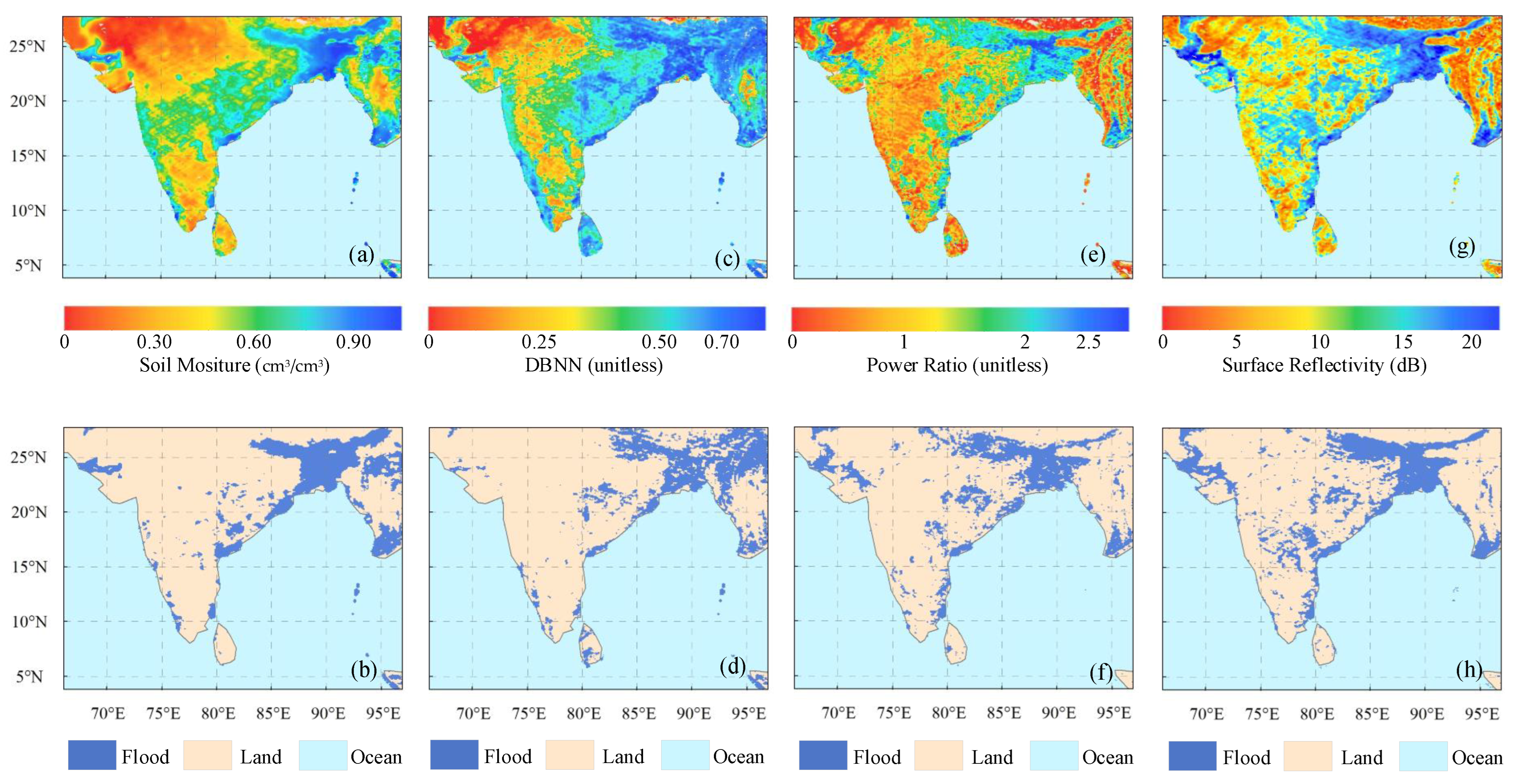
23] and uses the constant value of 2 as the threshold to distinguish between flood or land. In this study, the CYGNSS data ranging from 1 to 15 October 2020 are used as an example to investigate the inundation extent of the study area. In Figure 7, the inversion and classification results are presented for the flood monitoring in the study area, where the inversion results refer to the continuous values output by the methods, such as the surface reflectivity output of the SR method, and the classification results refer to the extent of flooding and land divided by the thresholds in various methods. In this study, the reference for judging the flood inundation range is obtained by the SMAP soil moisture threshold method due to the lack of measured data of the surface flood extent. Areas with soil moisture greater than 0.4 cm3/cm3 are classified as the inundated areas, and areas less than 0.4 cm3/cm3 are regarded as non-inundated areas [43]. Figure 7a shows the continuous spatial distribution of soil moisture, and Figure 7b shows flood inundation extent extracted by the soil moisture threshold method.
In this study, type I error, type II error, and overall accuracy are used to evaluate the classification results, which can be calculated as follows:
E 1 = a a + b + c E 2 = b a + b + c C = c a + b + c
where E 1 and E 2 denote the type I error and type II error, respectively. C represents the overall accuracy, a indicates the number of samples that misclassify water bodies as land, b is the number of samples that misclassify land as water bodies, and c is the number of correctly classified samples.
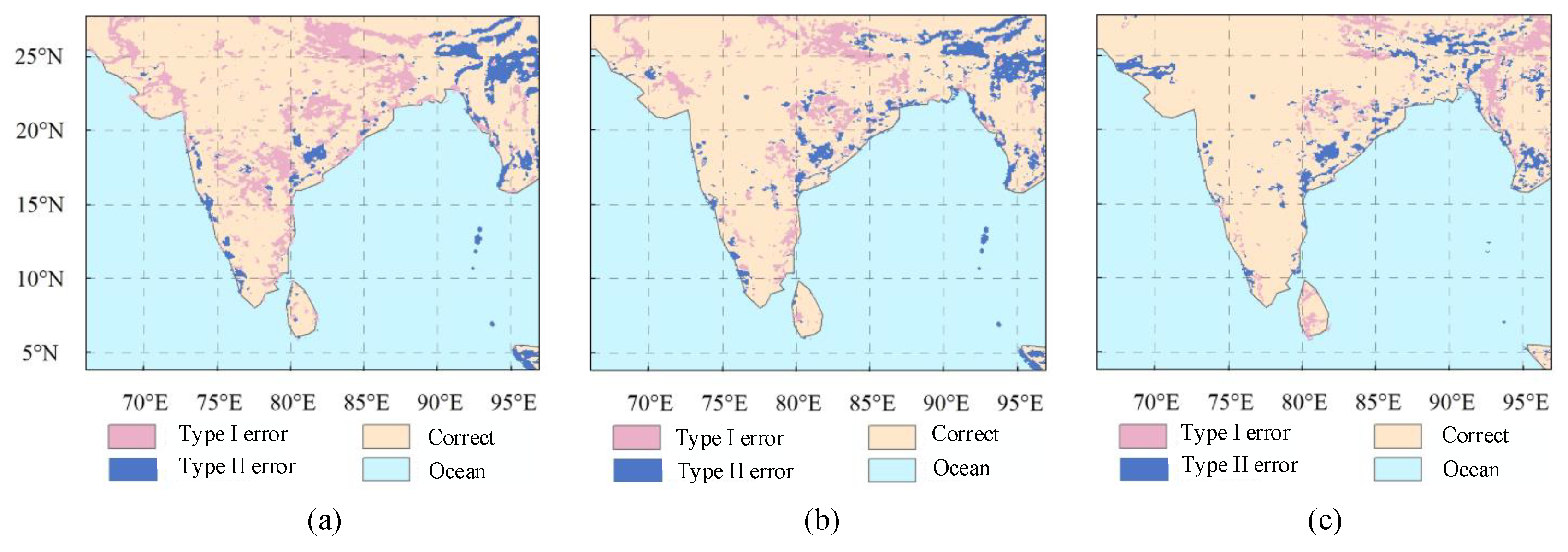
According to flood inundation extent delineated by the SMAP soil moisture threshold method, the overall accuracy, type I error, and type II error of the classification result of SR, PR, and DBNN methods are shown in Figure 8 and Table 4, where the DBNN method has the highest inversion accuracy of 85.4%, and the SR and PR methods have inversion accuracies of 80.17% and 81.34%, respectively. In addition, the DBNN method is additionally superior to SR and PR methods in terms of both type I error and type II error, which can be mainly attributed to the following aspects. Firstly, the DBNN model can fully exploit the underlying abstract features from DDMs, while combining the representative features as inputs of the model, which greatly enhances the utilization of GNSS-R data. Secondly, the DBNN model considers the influence of the vegetation factor on GNSS direct signals and reflected signals. However, it is worth noting that the DBNN model is fed with vegetation information from SMAP, whereas the previous SR and PR methods operate based on the CYGNSS data only.

4.2. Spatio-Temporal Analysis of Flood Inundation

In order to provide support for disaster-resistant activities in the study area, it is crucial to understand the development process of flood events. Therefore, the particularly severe flood incident occurring from May to September 2020 is selected as a flood monitoring case, and the experimental results retrieved by the DBNN model on CYGNSS data are shown in Figure 9 and Figure 10. Before the onset of the 2020 rainy season in the study area, the regions occupied by water bodies are mainly distributed in coastal areas such as Bangladesh, covering about 6.6% of the total land area. From 20 May 2020, the areas inundated by floods gradually expanded to Nepal and the northeast of India with the arrival of frequent rains. The flooded areas accounted for about 17.9% of the total area on 20 June 2020, and reached 28.7% by 20 July 2020. On 20 August 2020, the areas flooded reached their largest, covering around 34.8% of the total area. After 20 August 2020, the flooded areas gradually reduced because of the decrease in rainfalls. Observing the process of flood changes, we could find the increased area, which refers to the difference between the maximum flood area detected during the rainy season and the area of water bodies before the rainy season, accounting for 28.2% of the total study area, mainly in Nepal and the northeastern states of India. In particular, the proportion of the increased flood area in some states is calculated and summarized in Table 5, where Bihar State experienced the most severe flooding event with an increased area accounting for 89.92% of the total area, while Magway State had the smallest increased area, only covering about 5.50%.
Through further observation of Figure 9 and Figure 10, it can be found that the flooded areas are mostly located in Bangladesh, Nepal, and northeast of India, which is mainly caused by three factors; i.e., the large quantities of water vapor carried by the southwest monsoons, as well as the influence of topography and water systems. In terms of topography, the region is located at the southern foothills of the Himalayas and on the windward slope of the southwest monsoons. When the southwest monsoon is blocked by the northern mountains, it is forced to lift up and form topographic rain, leading to high rainfall in the study area. In terms of the water system, rainwater from the northern foothills is usually collected in the northeast of the study area, due to the low topography and dense river networks, making the region more vulnerable to the threat of flooding.

4.3. Discussion

Compared to SMAP data, the regions with more errors in the inversion results of CYGNSS data are mainly located in high altitude and inland permanent water regions, such as the Western Ghats and the Malwa plateau. The reason for such errors is that CYGNSS uses the DTU10 digital elevation model to calibrate the locations of specular points [23], which does not sufficiently consider the effect of land topography, resulting in high errors in the estimated positions of specular points with altitudes greater than 600 m on land. In addition, the difference in spatial resolution between CYGNSS data and SMAP data can also increase errors in the inversion results. For example, a small area of water may be identified by CYGNSS data, but not by SMAP data with a lower spatial resolution, which will increase the errors in inversion results.
Although the DBNN method could achieve a relatively higher inversion accuracy in flood monitoring, its accuracy would decrease in some special areas, such as flat areas. The DBNN method may misclassify the flat areas as water bodies because both of them have less surface roughness, thus producing similar coherent DDMs. In future research, inversion accuracy in flat areas is expected to be improved by extracting new physical features. In addition, considering that the DBNN method needs to learn an abundance of parameters and takes a large amount of computation to construct the optimal neural network model compared with the traditional methods, more lightweight models for flood monitoring should be anticipated to highly improve their operational efficiency in the future.

5. Conclusions

This study proposes a DBNN model for GNSS-R flood monitoring, which is mainly composed of a CNN module and a BP neural network module. The former is adopted to extract the underlying abstract features from DDMs, while the latter takes typical GNSS-R physical features and vegetation information as input. This kind of dual-branch neural network scheme can adequately combine GNSS-R physical features with the abstract features mined by CNN, which helps the DBNN model better utilize GNSS-R data for flood inversion and dynamic monitoring of inundation. Taking the study area in South Asia as an example, the effectiveness of the DBNN method was verified by comparison with the SR and PR methods. Then, the 2020 flood inundation in the study area was retrieved by the DBNN method, and it was found that DBNN had significant flood monitoring capabilities and could track the evolution process of floods over time. This study indicates that although CYGNSS is designed to observe ocean surface wind speed during hurricanes, it also possesses a promising future in flood monitoring applications.

Author Contributions

Conceptualization, methodology, D.S. and Q.Z.; software, Q.Z.; validation, writing—original draft preparation, D.S., Q.Z. and B.W.; writing—review and editing, D.S., Q.Z., C.Y. and J.X.; visualization, Q.Z.; funding acquisition, D.S. and B.W. All authors have read and agreed to the published version of the manuscript.

Funding

This work was supported by the National Key Research and Development Program of China under Grant 2019YFC1509202, the National Natural Science Foundation of China under Grant 61371189, 41701513, 41772350, and the Key Research and Development Program of Shandong Province under Grant 2019GGX101033.

Data Availability Statement

The CYGNSS datasets used during the study are available from NASA, https://podaac.jpl.nasa.gov (accessed on 10 September 2021). The SMAP datasets analyzed during the current study are available in https://nsidc.org/data/SPL3SMP_E/versions/4 (accessed on 16 October 2021).

Acknowledgments

The authors are grateful to the public CYGNSS data from the NASA Physical Oceanography Distributed Active Archive Center and SMAP data provided by National Snow and Ice Data Center.

Conflicts of Interest

There is no conflict of interest among the authors of this paper.

Abbreviations

The following abbreviations are used in this manuscript:
BPBack Propagation
CNNConvolutional Neural Network
CYGNSSCyclone Global Navigation Satellite System
DBNNDual-branch neural network
DDMDelay-Doppler map
DLDeep Learning
GNSS-RGlobal Navigation Satellite System-Reflectometry
PRPower ratio
SMAPSoil Moisture Active Passive satellite
SRSurface reflectivity

References

  1. Diakakis, M.; Boufidis, N.; Grau, J.M.S.; Andreadakis, E.; Stamos, I. A systematic assessment of the effects of extreme flash floods on transportation infrastructure and circulation: The example of the 2017 Mandra flood. Int. J. Disaster Risk Reduct. 2020, 47, 101542. [Google Scholar] [CrossRef]
  2. Messner, F.; Meyer, V. Flood damage, vulnerability and risk perception—Challenges for flood damage research. In Flood Risk Management: Hazards, Vulnerability and Mitigation Measures; Springer: Dordrecht, The Netherlands, 2006; pp. 149–167. [Google Scholar]
  3. Sharafi, S.; Kamangir, H.; King, S.A.; Safaierad, R. Effects of extreme floods on fluvial changes: The Khorramabad River as case study (western Iran). Arab. J. Geosci. 2021, 14, 1140. [Google Scholar] [CrossRef]
  4. Brivio, P.; Colombo, R.; Maggi, M.; Tomasoni, R. Integration of remote sensing data and GIS for accurate mapping of flooded areas. Int. J. Remote Sens. 2002, 23, 429–441. [Google Scholar] [CrossRef]
  5. Drusch, M.; Del Bello, U.; Carlier, S.; Colin, O.; Fernandez, V.; Gascon, F.; Hoersch, B.; Isola, C.; Laberinti, P.; Martimort, P. Sentinel-2: ESA’s optical high-resolution mission for GMES operational services. Remote Sens. Environ. 2012, 120, 25–36. [Google Scholar] [CrossRef]
  6. Platnick, S.; King, M.D.; Ackerman, S.A.; Menzel, W.P.; Baum, B.A.; Riédi, J.C.; Frey, R.A. The MODIS cloud products: Algorithms and examples from Terra. IEEE Trans. Geosci. Remote Sens. 2003, 41, 459–473. [Google Scholar] [CrossRef] [Green Version]
  7. Yang, W.; Gao, F.; Xu, T.; Wang, N.; Tu, J.; Jing, L.; Kong, Y. Daily Flood Monitoring Based on Spaceborne GNSS-R Data: A Case Study on Henan, China. Remote Sens. 2021, 13, 4561. [Google Scholar] [CrossRef]
  8. Kuenzer, C.; Guo, H.; Huth, J.; Leinenkugel, P.; Li, X.; Dech, S. Flood mapping and flood dynamics of the Mekong Delta: ENVISAT-ASAR-WSM based time series analyses. Remote Sens. 2013, 5, 687–715. [Google Scholar] [CrossRef] [Green Version]
  9. Hein, G.W. Status, perspectives and trends of satellite navigation. Satell. Navig. 2020, 1, 22. [Google Scholar] [CrossRef] [PubMed]
  10. Rodriguez-Alvarez, N.; Camps, A.; Vall-Llossera, M.; Bosch-Lluis, X.; Monerris, A.; Ramos-Perez, I.; Valencia, E.; Marchan-Hernandez, J.F.; Martinez-Fernandez, J.; Baroncini-Turricchia, G. Land geophysical parameters retrieval using the interference pattern GNSS-R technique. IEEE Trans. Geosci. Remote Sens. 2010, 49, 71–84. [Google Scholar] [CrossRef]
  11. Chew, C.; Shah, R.; Zuffada, C.; Hajj, G.; Masters, D.; Mannucci, A.J. Demonstrating soil moisture remote sensing with observations from the UK TechDemoSat-1 satellite mission. Geophys. Res. Lett. 2016, 43, 3317–3324. [Google Scholar] [CrossRef]
  12. Foti, G.; Gommenginger, C.; Jales, P.; Unwin, M.; Shaw, A.; Robertson, C.; Rosello, J. Spaceborne GNSS reflectometry for ocean winds: First results from the UK TechDemoSat-1 mission. Geophys. Res. Lett. 2015, 42, 5435–5441. [Google Scholar] [CrossRef] [Green Version]
  13. Wang, C.; Yu, K.; Qu, F.; Bu, J.; Han, S.; Zhang, K. Spaceborne GNSS-R Wind Speed Retrieval Using Machine Learning Methods. Remote Sens. 2022, 14, 3507. [Google Scholar] [CrossRef]
  14. Guan, D.; Park, H.; Camps, A.; Wang, Y.; Onrubia, R.; Querol, J.; Pascual, D. Wind direction signatures in GNSS-R observables from space. Remote Sens. 2018, 10, 198. [Google Scholar] [CrossRef] [Green Version]
  15. Roberts, T.M.; Colwell, I.; Chew, C.; Lowe, S.; Shah, R. A Deep-Learning Approach to Soil Moisture Estimation with GNSS-R. Remote Sens. 2022, 14, 3299. [Google Scholar] [CrossRef]
  16. Azemati, A.; Melebari, A.; Campbell, J.D.; Walker, J.P.; Moghaddam, M. GNSS-R Soil Moisture Retrieval for Flat Vegetated Surfaces Using a Physics-Based Bistatic Scattering Model and Hybrid Global/Local Optimization. Remote Sens. 2022, 14, 3129. [Google Scholar] [CrossRef]
  17. Chen, S.; Yan, Q.; Jin, S.; Huang, W.; Chen, T.; Jia, Y.; Liu, S.; Cao, Q. Soil Moisture Retrieval from the CyGNSS Data Based on a Bilinear Regression. Remote Sens. 2022, 14, 1961. [Google Scholar] [CrossRef]
  18. Chew, C.; Reager, J.T.; Small, E. CYGNSS data map flood inundation during the 2017 Atlantic hurricane season. Sci. Rep. 2018, 8, 9336. [Google Scholar] [CrossRef]
  19. Wan, W.; Liu, B.; Zeng, Z.; Chen, X.; Wu, G.; Xu, L.; Chen, X.; Hong, Y. Using CYGNSS data to monitor China’s flood inundation during typhoon and extreme precipitation events in 2017. Remote Sens. 2019, 11, 854. [Google Scholar] [CrossRef] [Green Version]
  20. Chew, C.; Small, E. Estimating inundation extent using CYGNSS data: A conceptual modeling study. Remote Sens. Environ. 2020, 246, 111869. [Google Scholar] [CrossRef]
  21. Clarizia, M.P.; Pierdicca, N.; Costantini, F.; Floury, N. Analysis of CYGNSS data for soil moisture retrieval. IEEE J. Sel. Top. Appl. Earth Obs. Remote Sens. 2019, 12, 2227–2235. [Google Scholar] [CrossRef]
  22. Unnithan, S.K.; Biswal, B.; Rüdiger, C. Flood inundation mapping by combining GNSS-R signals with topographical information. Remote Sens. 2020, 12, 3026. [Google Scholar] [CrossRef]
  23. Al-Khaldi, M.M.; Johnson, J.T.; Gleason, S.; Loria, E.; O’Brien, A.J.; Yi, Y. An algorithm for detecting coherence in cyclone global navigation satellite system mission level-1 delay-Doppler maps. IEEE Trans. Geosci. Remote Sens. 2020, 59, 4454–4463. [Google Scholar] [CrossRef]
  24. Morris, M.; Chew, C.; Reager, J.T.; Shah, R.; Zuffada, C. A novel approach to monitoring wetland dynamics using CYGNSS: Everglades case study. Remote Sens. Environ. 2019, 233, 111417. [Google Scholar] [CrossRef]
  25. Dong, Z.; Jin, S. Evaluation of the land GNSS-Reflected DDM coherence on soil moisture estimation from CYGNSS data. Remote Sens. 2021, 13, 570. [Google Scholar] [CrossRef]
  26. Zhang, L.; Zhang, L.; Du, B. Deep learning for remote sensing data: A technical tutorial on the state of the art. IEEE Geosci. Remote Sens. Mag. 2016, 4, 22–40. [Google Scholar] [CrossRef]
  27. Rumelhart, D.E.; Hinton, G.E.; Williams, R.J. Learning representations by back-propagating errors. Nature 1986, 323, 533–536. [Google Scholar] [CrossRef]
  28. Entekhabi, D.; Njoku, E.G.; O’Neill, P.E.; Kellogg, K.H.; Crow, W.T.; Edelstein, W.N.; Entin, J.K.; Goodman, S.D.; Jackson, T.J.; Johnson, J. The soil moisture active passive (SMAP) mission. Proc. IEEE 2010, 98, 704–716. [Google Scholar] [CrossRef]
  29. Chew, C.; Small, E. Soil moisture sensing using spaceborne GNSS reflections: Comparison of CYGNSS reflectivity to SMAP soil moisture. Geophys. Res. Lett. 2018, 45, 4049–4057. [Google Scholar] [CrossRef] [Green Version]
  30. Gleason, S.; Ruf, C.S.; O’Brien, A.J.; McKague, D.S. The CYGNSS level 1 calibration algorithm and error analysis based on on-orbit measurements. IEEE J. Sel. Top. Appl. Earth Obs. Remote Sens. 2018, 12, 37–49. [Google Scholar] [CrossRef]
  31. Zavorotny, V.U.; Voronovich, A.G. Scattering of GPS signals from the ocean with wind remote sensing application. IEEE Trans. Geosci. Remote Sens. 2000, 38, 951–964. [Google Scholar] [CrossRef]
  32. Al-Khaldi, M.M.; Shah, R.; Chew, C.C.; Johnson, J.T.; Gleason, S. Mapping the Dynamics of the South Asian Monsoon Using CYGNSS’s Level-1 Signal Coherency. IEEE J. Sel. Top. Appl. Earth Obs. Remote Sens. 2020, 14, 1111–1119. [Google Scholar] [CrossRef]
  33. Lei, F.; Senyurek, V.; Kurum, M.; Gurbuz, A.C.; Boyd, D.; Moorhead, R.; Crow, W.T.; Eroglu, O. Quasi-global machine learning-based soil moisture estimates at high spatio-temporal scales using CYGNSS and SMAP observations. Remote Sens. Environ. 2022, 276, 113041. [Google Scholar] [CrossRef]
  34. O’Neill, P.E.; Chan, S.; Njoku, E.G.; Jackson, T.; Bindlish, R.; Chaubell, J. SMAP Enhanced L3 Radiometer Global Daily 9 km EASE-Grid Soil Moisture, 4th ed.; NASA National Snow and Ice Data Center Distributed Active Archive Center: Boulder, CO, USA, 2020. [Google Scholar]
  35. Boulder, Colorado USA. NASA National Snow and Ice Data Center Distributed Active Archive Center. Available online: https://nsidc.org/data/spl3smp_e/versions/4 (accessed on 16 October 2021).
  36. Chaubell, J.; Yueh, S.; Entekhabi, D.; Peng, J. Resolution enhancement of SMAP radiometer data using the Backus Gilbert optimum interpolation technique. In Proceedings of the 2016 IEEE International Geoscience and Remote Sensing Symposium (IGARSS), Beijing, China, 11–15 July 2016; pp. 284–287. [Google Scholar]
  37. Guo, W.; Du, H.; Cheong, J.W.; Southwell, B.J.; Dempster, A.G. GNSS-R wind speed retrieval of sea surface based on particle swarm optimization algorithm. IEEE Trans. Geosci. Remote Sens. 2021, 60, 4202414. [Google Scholar] [CrossRef]
  38. Chew, C.; Small, E. Description of the UCAR/CU soil moisture product. Remote Sens. 2020, 12, 1558. [Google Scholar] [CrossRef]
  39. Yan, Q.; Huang, W. Spaceborne GNSS-R sea ice detection using delay-Doppler maps: First results from the UK TechDemoSat-1 mission. IEEE J. Sel. Top. Appl. Earth Obs. Remote Sens. 2016, 9, 4795–4801. [Google Scholar] [CrossRef]
  40. Goodfellow, I.; Bengio, Y.; Courville, A. Deep Learning; MIT Press: Cambridge, MA, USA, 2016. [Google Scholar]
  41. Gao, B.; Pavel, L. On the properties of the softmax function with application in game theory and reinforcement learning. arXiv 2017, arXiv:1704.00805. [Google Scholar]
  42. Aueb, T.R. One-vs-each approximation to softmax for scalable estimation of probabilities. Adv. Neural Inf. Process. Syst. 2016, 29. [Google Scholar]
  43. Rahman, M.S.; Di, L.; Shrestha, R.; Eugene, G.Y.; Lin, L.; Zhang, C.; Hu, L.; Tang, J.; Yang, Z. Agriculture flood mapping with Soil Moisture Active Passive (SMAP) data: A case of 2016 Louisiana flood. In Proceedings of the 2017 6th International Conference on Agro-Geoinformatics, Fairfax, VA, USA, 7–10 August 2017; pp. 1–6. [Google Scholar]
Figure 1. Schematic of the GNSS-R technique. GNSS satellites transmit signals to the Earth’s surface. The signal is reflected by the Earth’s surface and captured by GNSS-R receivers onboard low Earth-orbiting satellites. The specific locations of the specular points depend on the geometric positions of the transmitting and receiving satellites.
Remotesensing 14 05129 g001
Figure 2. (a) The coverage area of one CYGNSS satellite in a day. (b) The study area in South Asia.
Remotesensing 14 05129 g002
Figure 3. Flow chart of the inversion method.
Remotesensing 14 05129 g003
Figure 4. Mapping relationship between the spatial coordinate system and delay-Doppler coordinate system. The subfigure on the left depicts the spatial coordinate system. The ellipse and the curve represent a delay isoline and a Doppler shift isoline, respectively. The subfigure on the right represents the delay-Doppler coordinate system, where the blue and yellow delay Doppler pixels in DDMs correspond to one and two spatial points in the left subfigure, respectively, while white pixels represent the thermal noise pixels without corresponding spatial point. SP: the specular point.
Remotesensing 14 05129 g004
Figure 5. (a) DDM before removing the thermal noise pixels; (b) DDM after removing the thermal noise pixels.
Remotesensing 14 05129 g005
Figure 6. (a) Flooding monitoring process of DBNN method; (b) DBNN model structure. FC: full connection layer.
Remotesensing 14 05129 g006
Figure 7. The inversion and classification results for the flood monitoring in the study area. (a) Soil moisture values provided by SMAP mission and (b) flood inundation extent classified by threshold method, respectively. The inversion results of (c) DBNN method, (e) PR method, and (g) SR method. The classification result of (d) DBNN method, (f) PR method, and (h) SR method.
Remotesensing 14 05129 g007
Figure 8. (a) The difference image between SR classification result and SMAP classification result. (b) The difference image between PR classification result and SMAP classification result. (c) The difference image between DBNN classification result and SMAP classification result.
Remotesensing 14 05129 g008
Figure 9. The spatial distribution of the study area flood inundation retrieved by DBNN model on CYGNSS. The period spans from May to September 2020.
Remotesensing 14 05129 g009
Figure 10. The temporal variation process of the flooded area, spanning from May to September 2020. “CYGNSS-DBNN” indicates flood inundation area retrieved by DBNN method based on CYGNSS data, while “SMAP-Threshold” denotes flood inundation area classified by threshold method based on SMAP data.
Remotesensing 14 05129 g010
Table 1. Main parameters of CYGNSS satellite data.
ParametersUnitsComment
raw_countswattDDM bin raw counts
gps_tx_power_db_wdBiGPS Space Vehicle transmit power
rx_to_sp_rangemReceiver to specular point range
tx_to_sp_rangemTransmitter to specular point range
gps_ant_gain_db_idBiGPS Space Vehicle transmit antenna gain
sp_rx_gaindBiSpecular point receiver antenna gain
sp_latdegreeSpecular point latitude
sp_londegreeSpecular point longitude
sp_inc_angledegreeSpecular point incident Angle
Table 2. Main parameters of SMAP mission data.
ParametersUnitsComment
latitudedegrees_northLatitude of the center of the Earth based grid cell.
longitudedegrees_eastLongitude of the center of the Earth based grid cell.
soil_moisturecm3/cm3Representative soil moisture measurement for the Earth based grid cell.
surface_temperatureKelvinsTemperature at land surface based on GMAO GEOS-5 data
vegetation_opacityunitlessThe measured opacity of the vegetation used in retrievals in the grid cell.
roughness_coefficientunitlessA unitless value that is indicative of bare soil roughness used in retrievals within the 9 km grid cell.
Table 3. Features extracted from DDMs.
NumberFeatures SymbolFeatures Name
1DDMADDM average
2TESTail edge of slope
3LESLeading edge of slope
4SRSurface reflectivity
5PRPower ratio
6SNRSignal to noise ratio
7PeakDDM peak value
Table 4. Classification error and accuracy of PR and DBNN.
Type I Error (%)Type II Error (%)Accuracy (%)
SR10.769.0780.17
PR9.259.4181.34
DBNN7.297.1785.54
Table 5. The proportion of the increased flood area to the state area.
StateProportion (%)StateProportion (%)
West Bengal39.83Bihar89.92
Assam16.35Narayani Zone37.33
Rakhine State18.65Lumbini Zone41.79
Chattogram15.88Uttar Pradesh76.12
Karnali Zone25.92Odisha51.70
Seti Zone66.67Ayeyarwady45.12
Janakpur Zone31.84Yangon67.20
Sagarmatha Zone28.44Bago39.74
Bhojpur24.65Jharkhand65.25
Mechi Zone17.12Madhya Pradesh17.42
Sagaing12.26Chhattisgarh53.82
Rangpur19.57Magway5.50
Publisher’s Note: MDPI stays neutral with regard to jurisdictional claims in published maps and institutional affiliations.

