Time-Lagged Ensemble Quantitative Precipitation Forecasts for Three Landfalling Typhoons in the Philippines Using the CReSS Model, Part II: Verification Using Global Precipitation Measurement Retrievals

Abstract

In this study, high-resolution quantitative precipitation forecasts (QPFs) in lagged runs with a cloud-resolving model are evaluated for three typhoons in the Philippines: Mangkhut (2018), Koppu (2015), and Melor (2015), hitting northern Luzon, central Luzon, and the middle section of the Philippine archipelago, respectively. In Part I of this study, the QPFs were verified using 56 gauge observations on land over the Philippines. Here, in Part II, they are verified against the Global Precipitation Measurement (GPM) satellite estimates (also covering nearby oceans), using categorical scores in the same way. For each typhoon, rainfall valid at a selected 24 h period and the whole event (48 or 72 h) is examined. For 24 h rainfall inside the short range (lead time ≤ 72 h), good QPFs (with a threat score of ≥0.2) were produced for Koppu at 200 mm by almost all runs, and at 100 mm by all runs for Mangkhut, but only 22% of the runs for Melor. At longer lead times, good QPFs at 100 mm were also produced by all runs for Koppu, half of the runs for Mangkhut, and only 1 out of 16 runs for Melor. For whole events (48 or 72 h), the QPFs were similarly the best for Koppu, followed by Mangkhut, and least ideal for Melor. The quality of the GPM data during the three typhoons was found to be generally good and suitable for QPF verification, and the results were more stable and, thus, more reliable for the assessment of bias. However, the threat scores using the GPM dropped lower at high thresholds, and the results could become different from those obtained against the gauges (Part I), suggesting a much higher skill. Thus, verification using rain gauges is still needed toward high thresholds, especially over mountain regions where satellite estimates tend to exhibit larger errors.

1. Introduction

Located along the main path of tropical cyclones (TCs), or typhoons in the western North Pacific, the Philippines is the world’s most exposed country when it comes to the hazards of these fierce storms [1,2,3,4]. Thus, in addition to gale-force winds and storm surges near the centers of the TCs, e.g., [5,6,7], accurate quantitative precipitation forecasts (QPFs) for heavy rainfall are also important [8,9] and under high demand due to their associated hazards of flooding, inundation, landslides, and debris flow [10,11,12]. However, in modern numerical weather prediction (NWP), heavy-rainfall QPFs are still a highly challenging area [9,13], and very few studies have performed such tasks for TCs in the Philippines in a quantitative and objective manner thus far, e.g., [14,15,16].

In Taiwan, which is just north of the Philippines across the Luzon Strait, the development of typhoon QPFs began earlier, and there are more related studies in the literature. As Taiwan is mountainous and has steep topography (peaking at almost 4 km), it has long been recognized that the rainfall pattern brought by a TC in Taiwan is mainly controlled by the relative location of its center to the island due to topographic enhancements on the windward slopes facing the TC circulation [17,18,19], and, thus, the total rainfall is dictated by the track of the storm [20,21,22]. Partly owing to this rainfall mechanism phase-locked to the terrain, typhoon QPFs in Taiwan have been shown to be quite skillful within the short range (≤72 h) through deterministic high-resolution models [23,24,25], when the track errors are often within a reasonable range. Moreover, the skill scores are higher and, thus, the heavy rainfall is more predictable in larger events (in terms of rainfall) [23], including at high thresholds of ≥500 mm (per 24 h) [24,25].

As high resolution is required for QPFs [26] and it is not ideal to split the available computational resource among multiple members as usually adopted, e.g., [22], the time-lagged strategy [27] has been recommended and used by [28] for ensembles to account for the stochastic nature of NWP [29,30] and to obtain the probability information, e.g., [31,32,33]. In the past, time-lagged ensembles were mostly used for short-range forecasts, e.g., [34,35,36,37]. On the other hand, the system in [28] not only allows for high-quality QPFs comparable to those noted earlier at the short range, but with a range out to eight days, it also has the potential for QPFs at longer lead times (if the track is close enough). Essentially, these runs at longer lead times can provide different rainfall scenarios associated with different TC tracks, including the key information of a realistic “worst-case” scenario (e.g., with a direct hit), for the authority to start early preparations [28]. Later, as the lead time shortens and the uncertainty in tracks reduces, the most likely rainfall scenario emerges, as reflected in the temporal evolution of derived probabilities from successive runs. Then, the authority can arrange for proper adjustments. Of course, case-to-case variations exist in predictability due to the specific environment and flow pattern associated with each TC [26,28,38,39]. However, it should be pointed out that such time-lagged ensembles do not account for initial conditions and model uncertainty, and the earlier runs may have a lower skill.

Due to the close proximity and geological characteristics of the Philippines and Taiwan, one wonders how well a similar time-lagged ensemble system can predict typhoon QPFs for the Philippines. Such a study was recently carried out, and its first part (Part I) was reported [40]. As in [23,24,28,38,39], the 2.5 km cloud-resolving storm simulator (CReSS) [41,42] was used to perform QPFs for three typhoons that reached landfall through different parts of the Philippines (Figure 1a): typhoons (TYs) Mangkhut (2018), Koppu (2015), and Melor (2015). The tracks and QPFs were verified using categorical measures against 56 rain gauge observations. The performance was the best for Koppu, which penetrated central Luzon, as many runs within the short range exhibited high skills of up to 350–500 mm (observed peak amount = 695 mm in 72 h for the whole event). For Melor, which passed through the middle part of the Philippine archipelago, some members at the short range were also skillful at 200–350 mm (peak = 407 mm in 72 h). For Mangkhut, which struck northern Luzon and produced the most rainfall among the three TCs (based on rain gauges, 786 mm in 48 h), the rainfall was the least predictable. The best short-range member for it was skillful only up to 200 mm. At longer lead times beyond the short range, approximately one-third of the runs also produced quality QPFs up to 350 mm for both Koppu and Melor, but none for Mangkhut, due to larger northward track biases at such longer ranges. Thus, overall, a fair chance exists for decent and realistic QPFs at lead times of approximately 3–7 days in two (out of three) landfalling TCs in the Philippines, and the rain gauge verification results are encouraging [40].

While Part I was among the earliest studies to verify QPFs with high-resolution models for TC rainfall in the Philippines using objective and quantitative methods, a few issues can be further explored. First, the 56 rain gauges were from manned weather stations operated by the Philippine Atmospheric, Geophysical and Astronomical Services Administration (PAGASA) and scattered across the nation. They provided accurate rainfall measurements for model verification, but the density was not high compared to Taiwan (approximately 450 sites), and very few stations are located in the mountains (Figure 1b). Thus, the rainfall caused by the three TCs in the mountains might have not been well captured, and the QPF verification results could be more random and unstable. Since the time of the Tropical Rainfall Measuring Mission (TRMM) [43], many satellite-derived rainfall products have been put forward [44,45,46] and widely used in studies across a variety of spatial and time scales, e.g., [47,48], including those in the Philippines [49,50,51,52]. While these gridded datasets are estimates and may possess certain errors [50], the most notable being the underestimations in heavy rainfall over the terrain, e.g., [53,54,55,56], they do have the advantages of high resolution and even coverage over both land and ocean [43,44,45,46,49,52]. The latest such product is the Global Precipitation Measurement (GPM) mission [57,58], and its Integrated Multisatellite Retrieval for GPM (IMERG) product [52,53,59] was evaluated to be suitable for NWP evaluations over the Maritime Continent and the Philippines at daily and subdaily time scales [60]. Therefore, as our primary objective here in Part II, the high-resolution GPM IMERG data during the three typhoons are employed to verify their QPFs using the same methods as in Part I. The verification results are compared with those in Part I, which used the rain gauges [40], so as to assess the general quality of the GPM IMERG data during the three rather extreme TC rainfall events. This is our second objective. In addition, the three TCs were quite intense at landfall (at least category three on the Saffir–Simpson scale, Figure 1a), and the intensity predictions with the time-lagged ensemble are verified along with the probability information of heavy rainfall, both of which are aspects not covered in Part I [40].

The rest of this paper is arranged as follows. In Section 2, data and methodology are described, including the CReSS model, hindcast experiments, GPM data, and the verification of the model QPFs. In Section 3, Section 4 and Section 5, the time-lagged ensemble results in track, intensity, and QPFs for TYs Mangkhut (2018), Koppu (2015), and Melor (2015) are presented and discussed following this order, respectively. In Section 6, a further comparison and discussion of QPF results are given, and, finally, the conclusions are drawn in Section 7.

2. Data and Methodology

2.1. The CReSS Model and Hindcast Experiments

Since the numerical model, hindcast experiments, and methods to verify the model QPFs were all identical to those in Part I [40], these aspects were only described very briefly here, and the readers are encouraged to refer to Part I [40] for more details when needed. In this study, the CReSS model (version 3.4.2) of Nagoya University [41,42] was used for all hindcast experiments. It is a single-domain cloud-resolving model designed to simulate clouds and various weathers at high resolution, and, thus, treats all clouds only explicitly using a double-moment bulk cold-rain scheme based on [42,61,62,63,64,65] by option (

Table 1. Domain configuration and physical packages of the CReSS model in this study.

Map projection	Lambert conformal (center at 123°E, secant at 5°N and 20°N)
Grid spacing (km)	2.5 × 2.5 × 0.1–0.5695 (0.4) *
Grid dimension (x, y, z)	864 × 696 × 50
Domain size (km)	2160 × 1740 × 20
Forecast frequency	Every 6 h (at 0000, 0600, 1200, and 1800 UTC)
Forecast length	8 days (192 h)
IC/BCs	NCEP GFS 0.5° × 0.5° analyses and forecasts (26 levels)
Cloud microphysics	Double-moment bulk cold-rain scheme
PBL parameterization	1.5-order closure with turbulent kinetic energy prediction
Surface processes	Shortwave/longwave radiation and momentum/energy fluxes
Soil model	43 levels, every 5 cm to 2.1 m in depth

* The vertical grid of CReSS is uneven and stretched (smallest at the bottom) and the parentheses give the average value.

). At the subgrid scale, the turbulence in the planetary boundary layer (PBL) [66,67], as well as the radiation, momentum, and energy fluxes at the surface [68,69], were parameterized, the latter with aid from a substrate model [42].

The horizontal grid size was 2.5 km, as in [23,28,40], with 50 vertical levels at a mean spacing of 400 m (smallest at the bottom). With 864 × 696 grid points, the domain size was 2160 km × 1740 km (Table 1, Figure 2). For all CReSS runs, the initial and boundary conditions (IC/BCs) were from the National Centers for Environmental Prediction (NCEP) Global Forecast System (GFS) gross analyses and forecasts (0.5° × 0.5°, 26 levels) conducted every 6 h [70,71] (Table 1). For each of the three typhoons, hindcast experiments were run every 6 h out to a range of eight days (192 h), except every 12 h for some early runs for Mangkhut. Since only data available up to the initial time (t₀) of each run were used, our results were equivalent to performance in real time.

2.2. Observation Data for Model Verification

To verify different aspects of the model hindcasts, the following data were used. For the TC track and intensity, the best track data from the Joint Typhoon Warning Center (JTWC) and Japan Meteorological Agency (JMA) were used. For QPF verification, the GPM IMERG data (Final Run V06B) [64] were used, as mentioned. This dataset has high spatial and temporal resolutions of 0.1° × 0.1°, conducted every 30 min, and provides data as far back as 2000. During the production, quasi-Lagrangian time interpolation, gauge data, and climatological adjustments were performed [59]. At each grid point (0.1° apart) inside the area of verification (see Section 2.3), the GPM data every 30 min were summed over the selected periods during the three TCs, either 24, 48, or 72 h in length. For comparison and discussion, the results of the QPF verification in Part I [40] against 56 rain gauges (Figure 1b) were also referenced.

2.3. Verification of Model QPFs

Additionally, identical to Part I [40], the categorical measures were adopted as the main tool to verify model QPFs, so they were only briefly described here. The method is widely used for binary or dichotomous (yes/no) events, where an event in QPFs is defined as reaching a specified threshold at a given point. Using the 2 × 2 contingency table [72,73,74], the results of model forecasts at a set of N verification points could be classified into four categories: correct predictions of events (hit (H)), events observed but not predicted (miss (M)), events predicted but not occurred (false alarm (FA)), and correct predictions of no events (correct negative (CN)). Thus, N = H + M + FA + CN, and commonly used scores, such as the probability of detection (POD, of observed events), success ratio (SR, of forecast events), threat score (TS), and bias score (BS), could be computed [72,73,74], respectively, as

POD = H/(H + M),

(1)

SR = H/(H + FA),

(2)

TS = H/(H + M + FA), and

(3)

BS = (H + FA)/(H + M).

(4)

Since the four categories were exclusive to each other, one could see that the POD, SR, and TS were all fractions and ranged from 0 to 1, the higher the better. Additionally, the TS could be no higher than either the POD or SR. The BS, on the other hand, indicated underprediction (BS < 1) or overprediction (BS > 1) with the model relative to the observation, so a BS = 1 would be its best score. In the performance diagram, which used the SR and POD as its two axes, all four scores could be shown simultaneously [75]. Later, the discussion mainly focused on the TS and BS. In this study, the model QPFs were interpolated onto the observation sites using the bilinear method, and the scores were computed at seven fixed thresholds (0.05, 10, 50, 100, 200, 350, and 500 mm) as in Part I, so the results could be compared. In the large domain that encloses the entire Philippines (5.35°–18.75°N and 119.55°–126.95°E), there were 74 × 134 = 9916 GPM grid points, so the sampling rate was much higher compared to the rain gauges (56 sites).

Besides the categorical scores, the similarity skill score (SSS) measures the overall similarity between the observed and predicted rainfall patterns [39,40], and is defined as

$$\mathrm{SSS}=1-\frac{\frac{1}{N}{{\displaystyle \sum }}_{i=1}^N{\left(f_i-o_i\right)}^2}{\frac{1}{N}\left({{\displaystyle \sum }}_{i=1}^N{f}_i{}^2+{{\displaystyle \sum }}_{i=1}^N{o}_i{}^2\right)},$$

(5)

where f_i and o_i are the forecast and observed rainfall, respectively, at the ith point among N. Thus, using the mean squared error (MSE) to reflect similarity, the SSS was the skill score measured against the largest possible MSE, i.e., the one when the model rainfall never overlapped with the observation (such that f_i and o_i did not coexist and the second term on the right was equal to one). Thus, 0 ≤ SSS ≤ 1 (the higher the better) and SSS = 1 meant a perfect match, where f_i = o_i at all of the points. As the categorical scores, the SSS was also computed at the observation points.

3. Time-Lagged Ensemble QPFs for TY Mangkhut (2018)

3.1. Track and Intensity of TY Mangkhut (2018)

Using the method described in Section 2, a total of 19 hindcast experiments was performed for TY Mangkhut (2018) up to the initial time at 1200 UTC on 14 September every 6 h, except at 0000 and 1200 UTC, only during 9–10 September as in Part I [40]. In Figure 2a, the predicted tracks are shown along with the JTWC’s best track. For Mangkhut that reached landfall in northern Luzon at approximately 1800 UTC on 14 September at a translation speed of approximately 30 km h⁻¹ (also Figure 1a), the earlier predictions determined during 9–11 September had northward biases that generally reduced with time, whereas the track errors afterwards were quite small and all within 80 km at landfall (Figure 2a). For more details in track errors, the readers are referred to Part I [40].

In Figure 3a, the intensity forecasts for Mangkhut are shown in both the minimum central mean sea level pressure (MSLP) and near-center maximum surface wind speed (at 10 m height). Besides the JTWC’s best track (black), data from the JMA (gray) were also plotted for comparison, but the latter used 10 min averages for the wind speed. As the only category five storm to make landfall among the three cases (Figure 1a), the JMA estimated a steady central MSLP of 905 hPa and wind speed of 56.5 m s⁻¹ up to landfall for Mangkhut, while the JTWC estimates were more variable with time, but at 911 hPa and 72 m s⁻¹ at landfall (Figure 3a). Except for the one at 0000 UTC on 14 September, all the lagged hindcasts produced a minimum central MSLP between 887 and 913 hPa at or near landfall with good agreement, including those during 9–10 September. In terms of peak surface wind speed (Figure 3b), again, the one at 0000 UTC on 14 September was the weakest (54 m s⁻¹), while all other runs reached 57–67 m s⁻¹ near landfall. The highest model wind speed was 70 m s⁻¹ and was produced by the run at 0600 UTC on 11 September, as the TC center missed landfall in Luzon (see Figure 2a). Thus, in wind speed, almost all hindcasts exceeded the JMA’s estimates, but could not fully match the JTWC’s best track data, with a deficit of approximately 5–15 m s⁻¹ at landfall (Figure 3b).

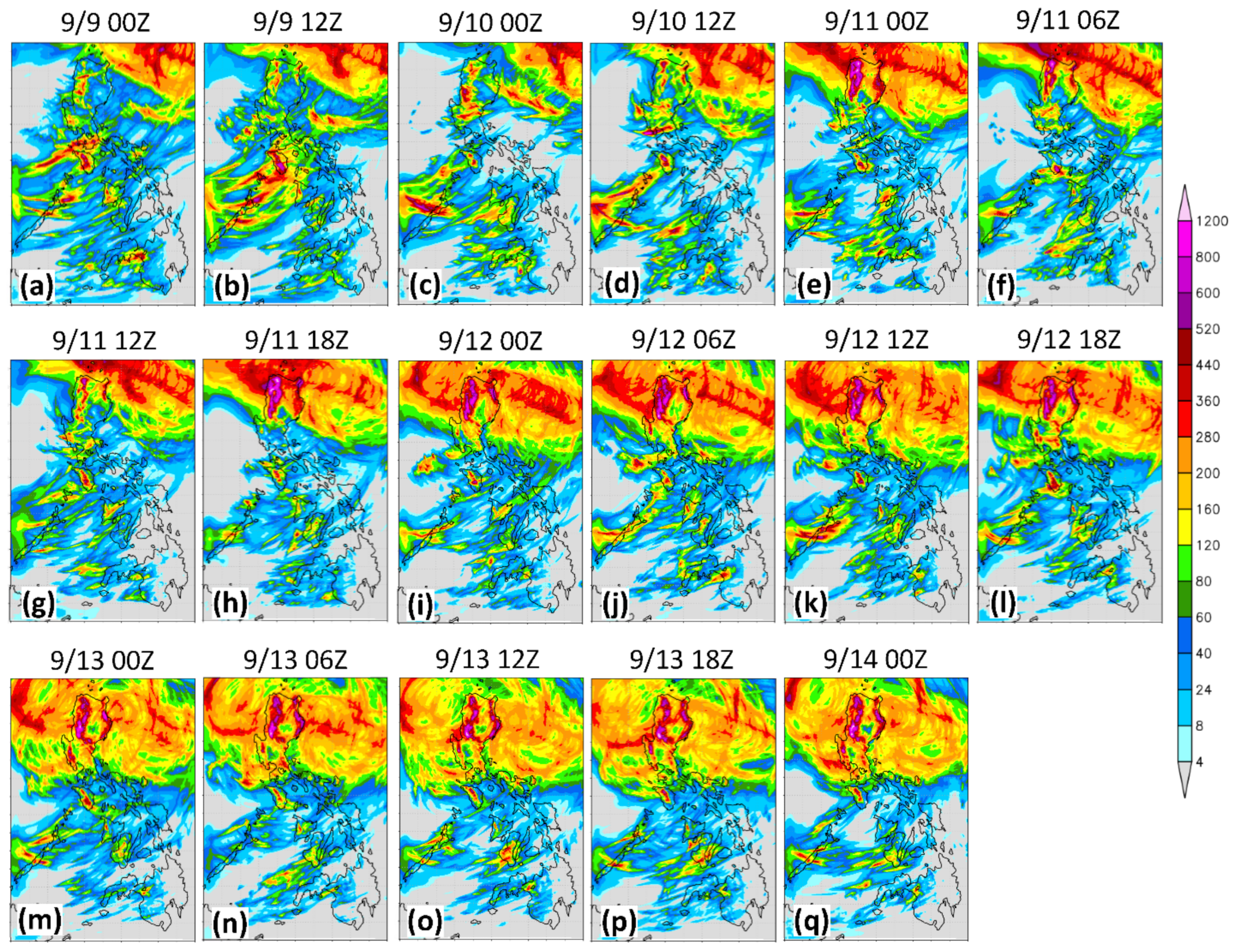
3.2. Observed and Predicted Rainfall of TY Mangkhut (2018)

The rainfall distributions over the Philippines and nearby oceans in the GPM retrievals during TY Mangkhut (2018) are shown in Figure 4 for 14 and 15 September and also the combined 48 h period. On 14 September (Figure 4a), the GPM depicted a peak daily rainfall of 451.5 mm approximately 150 km off the eastern coast of Luzon. Over land, the maximum was approximately 250 mm near 17°N along the Sierra Madre Mountain (SMM). On 15 September after Mangkhut reached landfall, the peak daily rainfall on land was 337.9 mm over the Cordillera Central Mountain (CCM, Figure 4b). When summed together over two days, the maximum rainfall offshore reached 455.2 mm and the CCM region also received over 280 mm, with peaks reaching approximately 400 mm (Figure 4c). Among all the gauge sites on land [40], 785.8 mm was observed over 14–15 September at Baguio, which was at an elevation of 1.5 km over the southwestern CCM (see Figure 1b). Therefore, while the overall rainfall pattern from Mangkhut in GPM, with significant amounts north of approximately 14.5°N in Luzon, should have been representative [60], the peak amount near Baguio might have been underestimated [50,52,53,76]. For TY Morakot (2009), associated with extreme rainfall in Taiwan, ref. [55] also found underestimations in several satellite products, especially in mountain regions.

Figure 5 presents the distributions of model QPFs with the lagged runs for the 48 h period of 14–15 September during Mangkhut, with t₀ between 0000 UTC on 9 September and 0000 UTC on 14 September. While a few panels were shown in Part I [40], they serve as an example to examine the QPF’s overall quality. Compared to Figure 4c, it was evident that the TC-associated rainfall in the early runs during 9–11 September was displaced northward due to track biases (Figure 5a–h). The TC center started to reach landfall in northern Luzon since 12 September (in t₀), and the overall rainfall regions became better predicted (Figure 5i–q). On Luzon, when track errors were small, most rainfall was produced over the CCM and SMM quite consistently with the lagged runs, in good agreement with the GPM in pattern. However, many members during 12–14 September produced rainfall amounts reaching 800–1000 mm over the CCM near Baguio (and ~600–800 mm along the SMM), considerably higher than the GPM estimated (~400 mm), but close to the rain gauge measurement of 785.8 mm at Baguio [40]. Over the ocean east of Luzon, the model rainfall was maximized along the eyewall just to the south and north of the center (e.g., Figure 5a–l), as one would expect for an intense, westward-moving TC such as Mangkhut. Presumably correct, this model rainfall characteristic was not well reflected in the GPM retrieval. Near 16.5°N 123.5°E, where a peak of 455.2 mm was seen in the GPM data (Figure 4c), most hindcast runs could only produce approximately 300–350 mm in the area, even with a good track (Figure 5). Nonetheless, in the last several runs during 13–14 September, the overall rainfall distribution did appear to improve (Figure 5m–q).

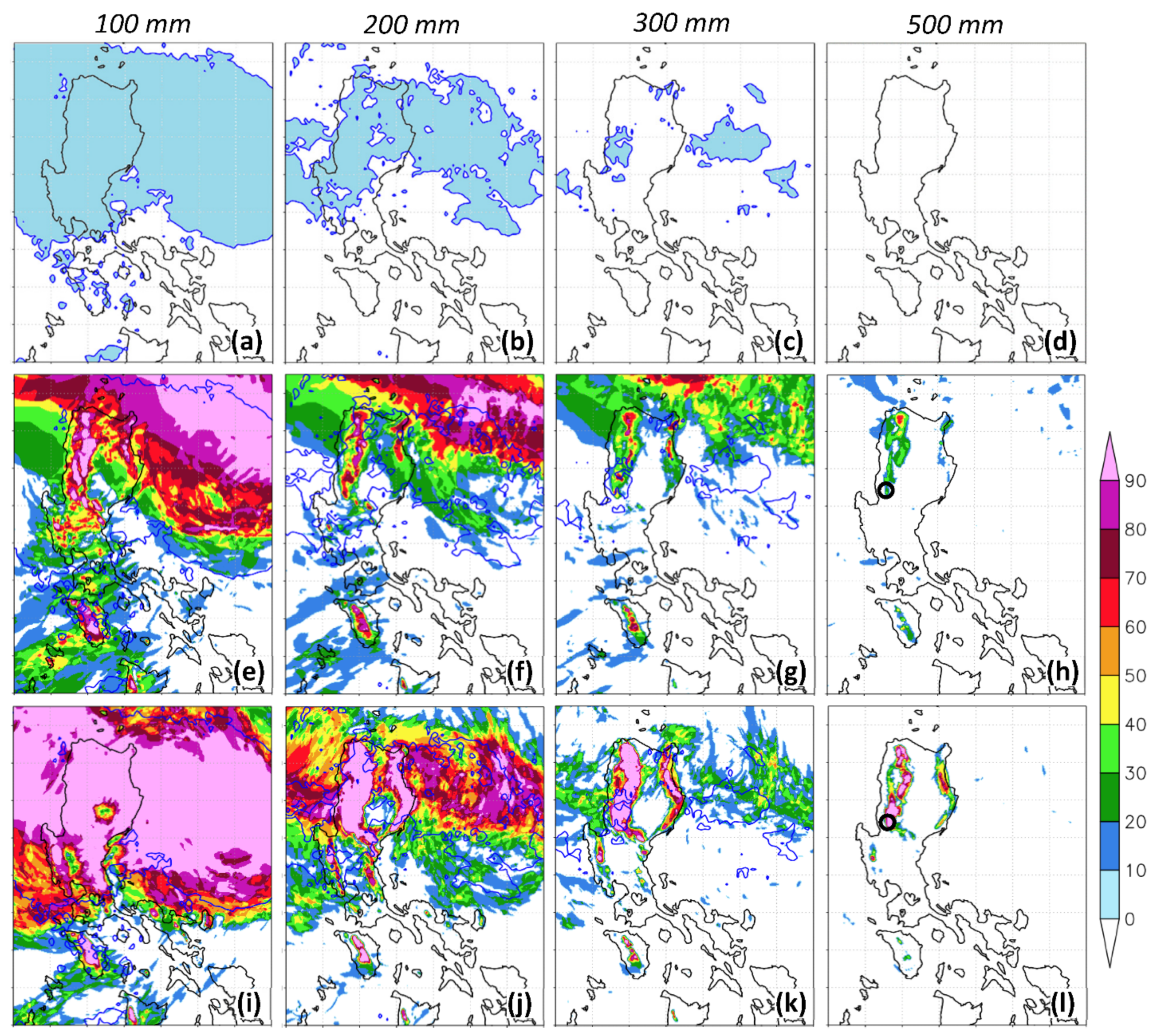
3.3. Heavy Rainfall Probabilities of TY Mangkhut (2018)

One distinct advantage of the time-lagged ensemble compared to deterministic forecasts was the availability of probability information, an aspect not examined in Part I [40]. In Figure 6, the probabilities of heavy rainfall reaching thresholds of 100, 200, 300, and 500 mm from TY Mangkhut (2018) for the period of 14–15 September (48 h), as derived from the first eight (Figure 6e–h) versus the last nine members (Figure 6i–l) in Figure 5, were compared with the actual regions in the GPM retrieval (Figure 6a–d). At the lowest selected threshold of 100 mm (per 48 h), a wide swatch in the GPM was seen to meet the criterion, roughly from 14.5°N to the Luzon Strait (Figure 6a). Due to the track bias, the high-probability region (say, ≥70%) derived from the first eight members (those executed during 9–11 September) was also displaced northward (Figure 6e). This error was corrected in the last nine members (those with t₀ at and after 0000 UTC on 12 September), as the region of ≥80% matched well with the observation (Figure 6i). When the threshold was raised to 200 mm, the swatch to reach this value in the GPM became narrower and covered roughly the northern half of Luzon (Figure 6b). Again, the first eight members had the high-probability area too far north (over the Luzon Strait), and the area was shifted back south in the last nine members (Figure 6f,j). In Figure 6j, both the CCM and SMM had over a 90% chance to receive a total amount of ≥200 mm, in good agreement with the GPM. However, the probabilities in some offshore areas east of Luzon were below 60% and not very high, reflecting the underprediction in rainfall amounts there (compared to the GPM).

At 300 mm, the GPM showed, roughly, only two regions to reach this amount: over the offshore ocean east of Luzon and in southern CCM surrounding Baguio on land (Figure 6c). For the offshore region, no more than 30% of the first eight members produced 300 mm with their track biases, while the percentages of ≤50% from the last nine members were not much higher, potentially due to the underprediction noted above (Figure 6g,k). Over land, on the other hand, the likelihood of rainfall reaching 300 mm over the CCM (and SMM) rose significantly as the lead time shortened, from below 60–70% in the first eight to over 90% in the last nine members. At the highest threshold of 500 mm, which was not reached anywhere in the GPM (Figure 6d), the earlier predictions still yielded an approximately 20–40% chance for their occurrence near Baguio (Figure 6h), and the likelihood further increased to approximately 90% in the last nine runs (Figure 6l). As discussed, even though the GPM only indicated approximately 360 mm in the southern CCM (Figure 4c), little doubt existed that this value from Mangkhut was underestimated (likely in the SMM as well) [50,52,53,76], as the rain gauge at Baguio recorded almost 800 mm. Therefore, the probability information over the mountain regions of Luzon for TY Mangkhut (2018) appeared to be much improved in the last nine runs (Figure 6). This result for Mangkhut was quite encouraging, and was achieved because the effect of a topographic enhancement in mountain areas could be properly simulated in high-resolution models. Linked to this enhancement, the hazards of flash floods and mud/debris flows were often higher in the mountains. On the other hand, the probability estimates over the ocean east of Luzon were likely on the low side, even with the later members with small track errors.

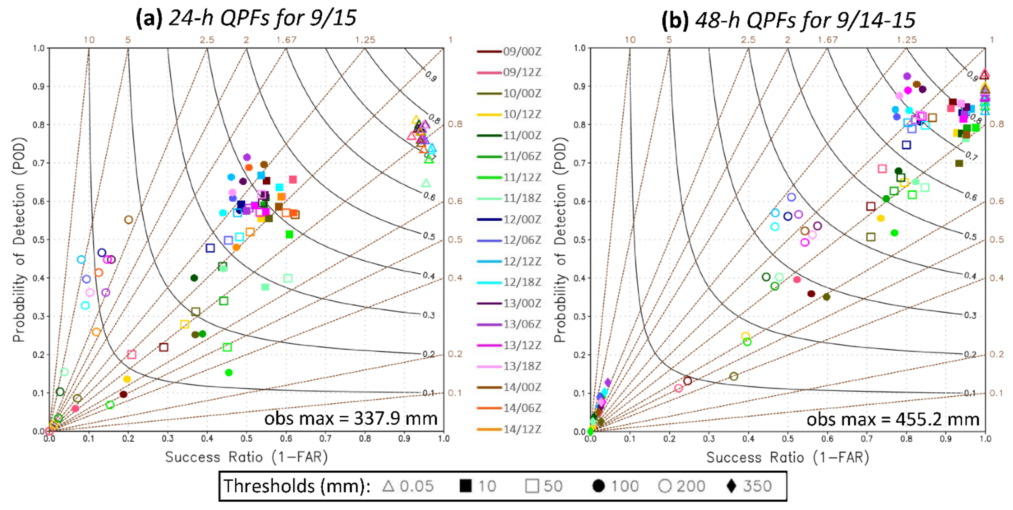
3.4. Objective Skill Scores of QPFs for TY Mangkhut (2018)

In this subsection, the categorical statistics obtained following the method described in Section 2.2 are presented, for 24 h QPFs targeted on 15 September (0000-2400 UTC, Figure 7a) and 48 h QPFs valid for 14–15 September (Figure 7b) during Mangkhut. As mentioned, the GPM retrievals were treated as the ground truth here, and, later, the results were compared with the same statistics from Part I [40] against the rain gauge measurements. On 15 September, the peak 24 h rainfall in GPM was 337.9 mm near Baguio in the CCM (see Figure 4b) rather than offshore, and this was why this date was chosen. In Figure 7a, the TS values from the lagged runs were clustered together at low thresholds, and were mostly 0.7–0.8 at 0.05 mm (per 24 h). Toward higher thresholds, the TSs decreased and the points became less concentrated, and were approximately 0.15–0.4 at 50 mm and ≤0.17 at 200 mm. Since the next threshold at 350 mm had already exceeded 337.9 mm, it was not a valid threshold to examine [40]. In the BS, most data points were between 0.5 and 1.5, thus, suggesting reasonable rain area sizes, except at 200 mm, where some members exhibited overprediction with BSs of 2–5.

Figure 7a could be compared with the same statistics for 15 September, but against the rain gauges, i.e., Figure 5b in Part I [40].

Table 2. Comparison of mean TS values and their range (maximum minus minimum) with the CReSS hindcasts for TY Mangkhut (2018) obtained against the GPM retrievals (left) and the rain gauges (right) in each category: 24 h (top half, for 15 September) and 48 h QPFs (bottom half, for 14–15 September, both in UTC) within the short range for the day 1 forecast (t₀ ≤ 48 h before the beginning of accumulation) and at longer ranges beyond. For each range group, the number of lagged runs was given in the parentheses and the three highest thresholds available were selected (based on the observed peak rainfall amount). Bold faces indicate the better result between the two data sources: a higher score but smaller range (except for mean TS = 0).

Mangkhut	Against GPM				Against Rain Gauges
24 h QPFs	Obs. Max	Threshold (mm)			Obs. Max	Threshold (mm)
	(mm)	50	100	200	(mm)	50	100	200
t0 within 48 h (7)
Mean TS	337.9	0.39	0.39	0.12	535.6	0.30	0.42	0.21
Range of TS		0.08	0.13	0.09		0.13	0.46	1.00
t0 beyond 48 h (12)
Mean TS	337.9	0.24	0.22	0.04	535.6	0.18	0.12	0.00
Range of TS		0.24	0.34	0.12		0.30	0.17	0.00
48 h QPFs	Obs. Max.	Threshold (mm)			Obs. Max.	Threshold (mm)
	(mm)	100	200	350	(mm)	100	200	350
t0 within 48 h (9)
Mean TS	455.2	0.72	0.36	0.02	785.8	0.29	0.27	0.00
Range of TS		0.10	0.05	0.02		0.20	0.34	0.00
t0 beyond 48 h (8)
Mean TS	455.2	0.43	0.18	0.01	785.8	0.15	0.12	0.00
Range of TS		0.29	0.20	0.02		0.21	0.29	0.00

(top half) also summarizes the comparison at three thresholds in mean TSs and their range among the runs. One could see that the TS values here tended to be higher at lower thresholds within the short range (t₀ inside 48 h from the beginning of accumulation), and also up to 200 mm (per 24 h) at longer ranges. This suggested better results in the rainfall region when the dense and gridded GPM data not confined to land areas were adopted. With 9916 total points, the TS values also often had smaller ranges and were, thus, more stable when using the GPM data. On the other hand, two runs were able to produce TS = 1 and 0.5 at 200 mm (at Baguio) against the rain gauges at the short range [40]; thus, they performed better at thresholds of ≥100 mm (Table 2, top half). Since many points reached this amount in the GPM (Figure 4b), such high TSs at higher thresholds would be difficult to achieve. Beyond the short range, the more stable results using the GPM tended to be better for Mangkhut, as the larger track errors prevented good QPFs at Baguio against the gauges [40]. The BSs in Figure 7a also indicated little bias in the rain area size from 0.05 to 100 mm, but the rain gauge results [40] suggested an overprediction by most members (1 ≤ BS ≤ 2.5). Thus, as one might anticipate, using satellite retrievals or rain gauges could produce somewhat different results.

The categorical scores for the 48 h QPFs over 14–15 September for Mangkhut are shown in Figure 7b, where the peak amount in GPM was 455.2 mm over the ocean (Figure 4c). Again, the data points at low thresholds were fairly concentrated, and the TSs were approximately 0.83–0.93 (and SR = 1) at 0.05 mm (per 48 h). At higher thresholds, the scores of all the runs executed during 12–14 September were confined to 0.63–0.73 at 50 mm and 0.33–0.39 at 200 mm, respectively. Only before 12 September, when the northward track bias was larger (eight runs), the TSs were lower (Figure 7b), and typically more so in earlier runs. Interestingly, in most runs, their TSs at 100 mm were higher than those at 50 mm, since the rain area reaching 100 mm was more confined, mostly north of 14°N (Figure 4c). At the highest threshold of 350 mm (per 48 h), the TS values all dropped to below 0.02, linked to the general underprediction over the ocean where rainfall in the GPM reached 350 mm in Figure 4c, as discussed earlier in Section 4.1.

If Figure 7b was compared to the same statistics (for 48 h QPFs) at the same thresholds using rain gauge data in Part I [40] (their Figure 5c), one could see that the TS values were almost all exclusively higher with smaller ranges here using the GPM (Table 2, bottom half). The differences were smaller at 0.05 and 10 mm, but were larger at higher thresholds, and maximized at 100 mm, where TSs using the GPM were higher by approximately 0.35–0.55. Here, at 100 mm, the range of TS values was 0.29 from runs beyond the short range, and although somewhat larger than that in Part I (0.21), it reflected the fact that the TSs could go much higher than those using the gauges. Additionally, even though the TSs were low at 350 mm in Figure 7b, they were all zero (no hits) when verified against the gauges in Part I [40]. Thus, for Mangkhut, the TSs using the GPM tended to be higher, except at short range over 100–200 mm, when the rainfall near Baguio could be captured. In [40], the BSs were mostly over 1–2.5 and, thus, indicated overprediction, but Figure 7b suggests no such tendency, or even a slight underforecast across the lower thresholds from 0.05 to 50 mm. These differences arose because the GPM data had a much higher sampling rate in space (more points), also covered the nearby oceans, and possessed some biases of their own.

Using the SSS as the measure for the overall skill of the QPFs (Figure 8a), the scores for the two day totals (of 14–15 September) over the large domain (solid black) showed gradual improvements from approximately 0.62 to 0.84 from 0000 UTC 9 September to 0000 UTC 12 September, then stayed quite stable until 0000 UTC 14 September. If only the QPFs for the first 24 h (14 September) were evaluated (solid red), the scores were also close. For some runs, the former scores were slightly higher, whereas the opposite was true for the others. If computed for the small domain surrounding Luzon (see Figure 4c), the scores (dashed) were slightly lower in both instances, by roughly 0.05. For 15 September, however, the SSS values were considerably lower, and rose from only 0.4–0.45 in the early runs to 0.65–0.73 since 12 September (solid blue, Figure 8a). Additionally, for the small domain, where most of the heavy amounts occurred (Figure 4b), the scores were considerably higher, by nearly 0.1–0.15 (dashed blue), in contrast to the QPFs for the first day and the two-day period. This result implied that when Mangkhut moved through the mountainous region of northern Luzon (on 15 September), the lagged runs tended to better predict such rainfall when phase-locked and enhanced with the CCM and SMM. In other words, the predictability of rainfall was higher there, similar to the mountains in Taiwan, e.g., [25].

The same SSS values, but computed against the 56 rain gauges over the Philippines, were plotted in Figure 8b, where the two curves for 14–15 September were shown in Part I [40]. The scores for the three verification periods were quite different from those obtained using the GPM data, and also from each other, except toward the end (at and after 1200 UTC on 13 September). The scores were the highest for 14 September, and rose from approximately 0.41 in the early runs to 0.79 in some later runs for both domains (red). For 15 September, on the contrary, the scores were the lowest (blue), and ranged from approximately 0.2 to 0.66. The scores for the 48 h QPFs (black) were in the middle and increased from approximately 0.35–0.4 to 0.7–0.75 near the end. In all three instances, the scores for the small domain were better than those for the large domain almost exclusively. Although all curves in Figure 8b exhibited a general trend to rise with a decreasing lead time, they were less stable and could have larger fluctuations from one run to the next, most likely linked to the fewer points available and, thus, offering a greater random impact from any of them. Overall, the SSS values for Mangkhut using the GPM data were higher and more stable compared to those using the rain gauge data, in agreement with earlier results from the categorical measures.

4. Time-Lagged Ensemble QPFs for TY Koppu (2015)

4.1. Track and Intensity of TY Koppu (2015)

The second case of TY Koppu (2015) moved due west and reached landfall at approximately 2300 UTC on 17 October at a slow translation speed of approximately 15 km h⁻¹, and then penetrated the middle part of Luzon, moved offshore, and turned north even more slowly (Figure 1a). For this case, 19 runs were carried out. The hindcasts during the first 2.5 days (before 1200 UTC on 15 October) also gradually deviated to the north and had an early northward turn (over land). Afterwards, the northward bias was alleviated and the track errors all became inside 75 km at landfall (Figure 2b). However, a premature northward turn still occurred, such that the TC center did not reach the western shore of Luzon until the last two runs, with t₀ at 0600 and 1200 UTC on 17 October.

TY Koppu (2015) reached landfall as a category four storm, its central MSLP was estimated by the JTWC to decrease from 993 hPa during 13–14 October to 926 hPa at 1200 UTC on 17 October before landfall (Figure 3c). The JMA gave a similar value of 925 hPa at 1800 UTC on 17 October. At landfall, the estimates were 942 and 938 hPa, respectively. The early hindcast runs during 13–15 October could reach a central MSLP of 908–918 hPa before landfall, which was lower than both best track estimates. Starting from 0000 UTC on 16 October, the lowest central MSLPs reached were 925–932 hPa, and were closer to the estimates, while the run at 0600 UTC on 17 October could only hit 939 hPa (Figure 3c). At the time of actual landfall (2300 UTC on 17 October), the predicted central MSLP of Koppu had a large range of 910–960 hPa, but the ones since 1200 UTC on 15 October tended to be closer to the best tracks near 940 hPa. In terms of wind speed (Figure 3d), the peak intensity of Koppu prior to landfall was estimated to be 66.5 m s⁻¹ by the JTWC and 51 m s⁻¹ by the JMA. Essentially, nearly all the lagged runs produced a peak wind speed between 59 and 65 m s⁻¹ prior to landfall, so they exceeded the JMA data and almost matched the JTWC estimate, including the earlier runs. The only two exceptions were the latest runs at 0600 and 1200 UTC on 17 October (54–55 m s⁻¹), when the model TC was already close to landfall. Overall speaking, the model performed quite well in capturing the intensity of Koppu, compared to Mangkhut.

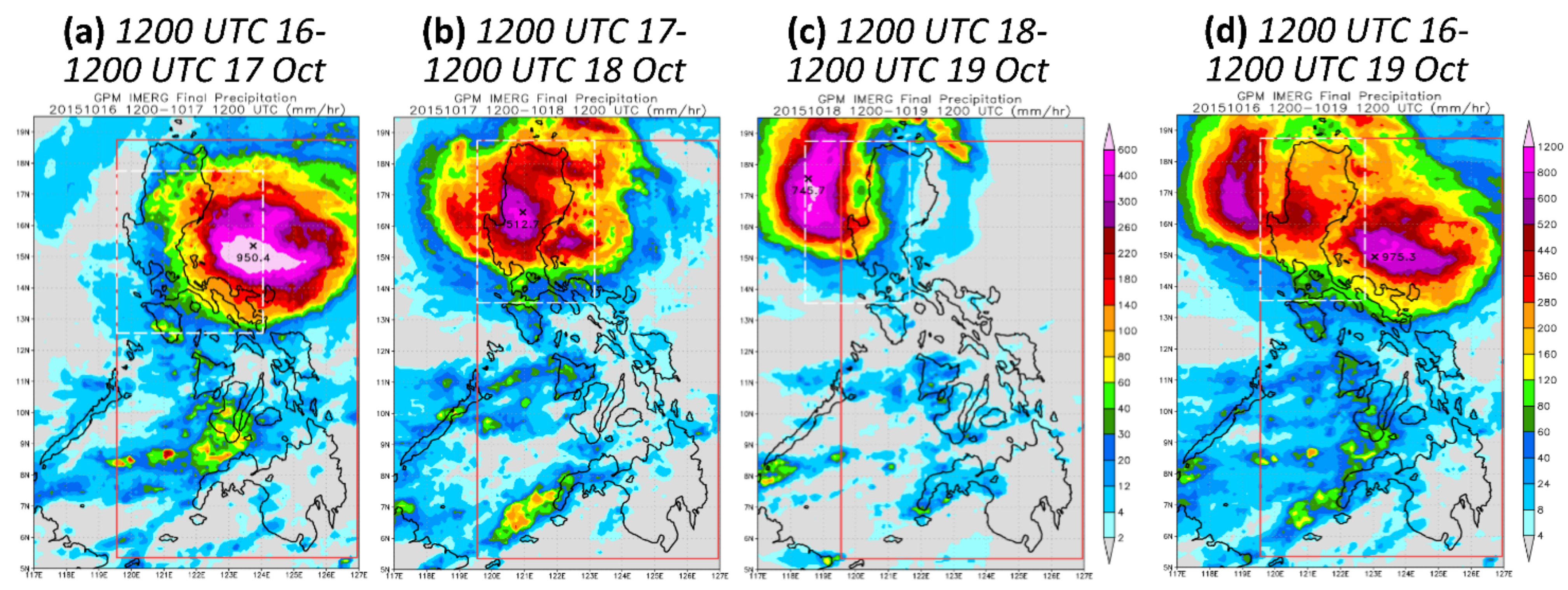
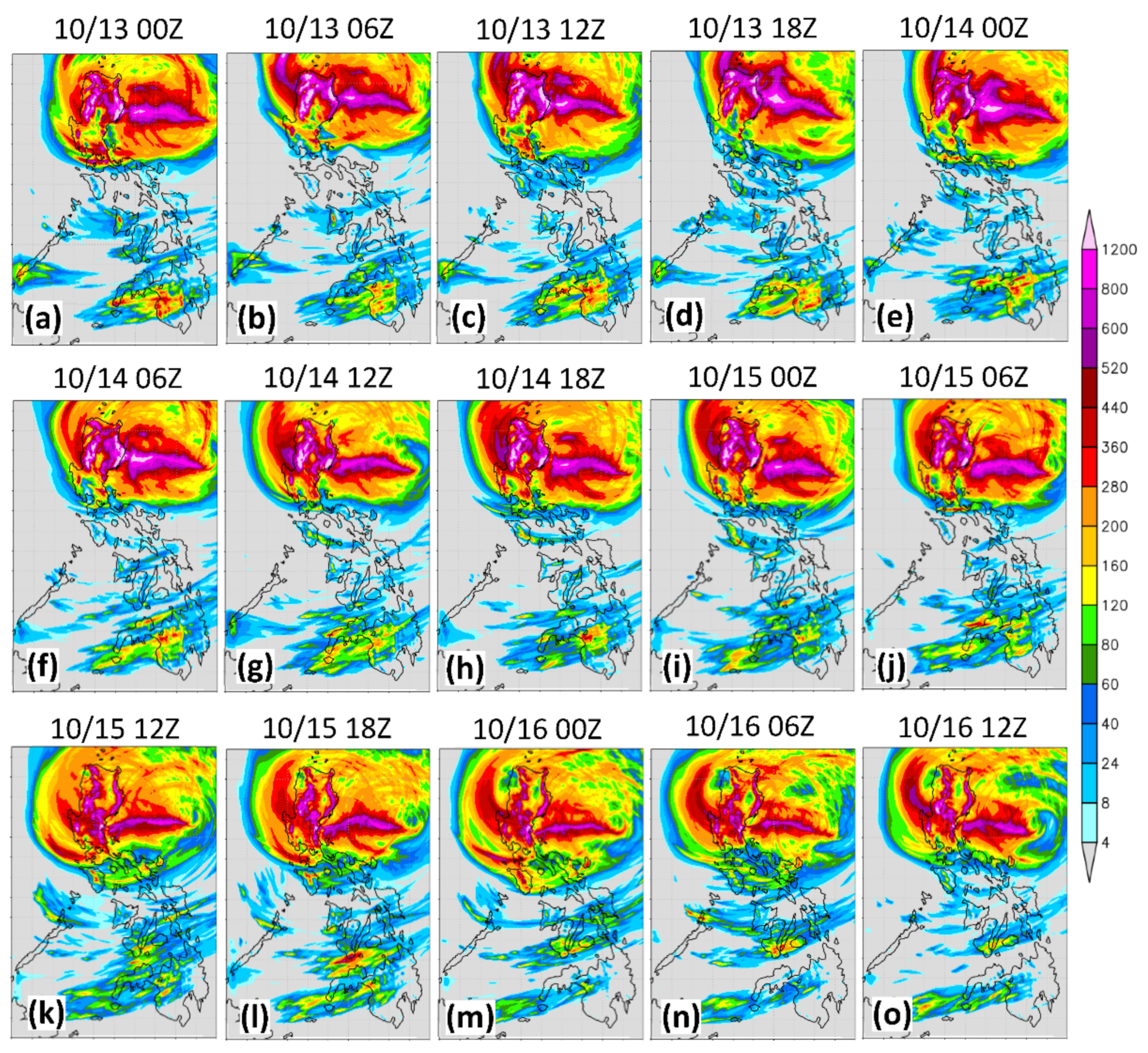
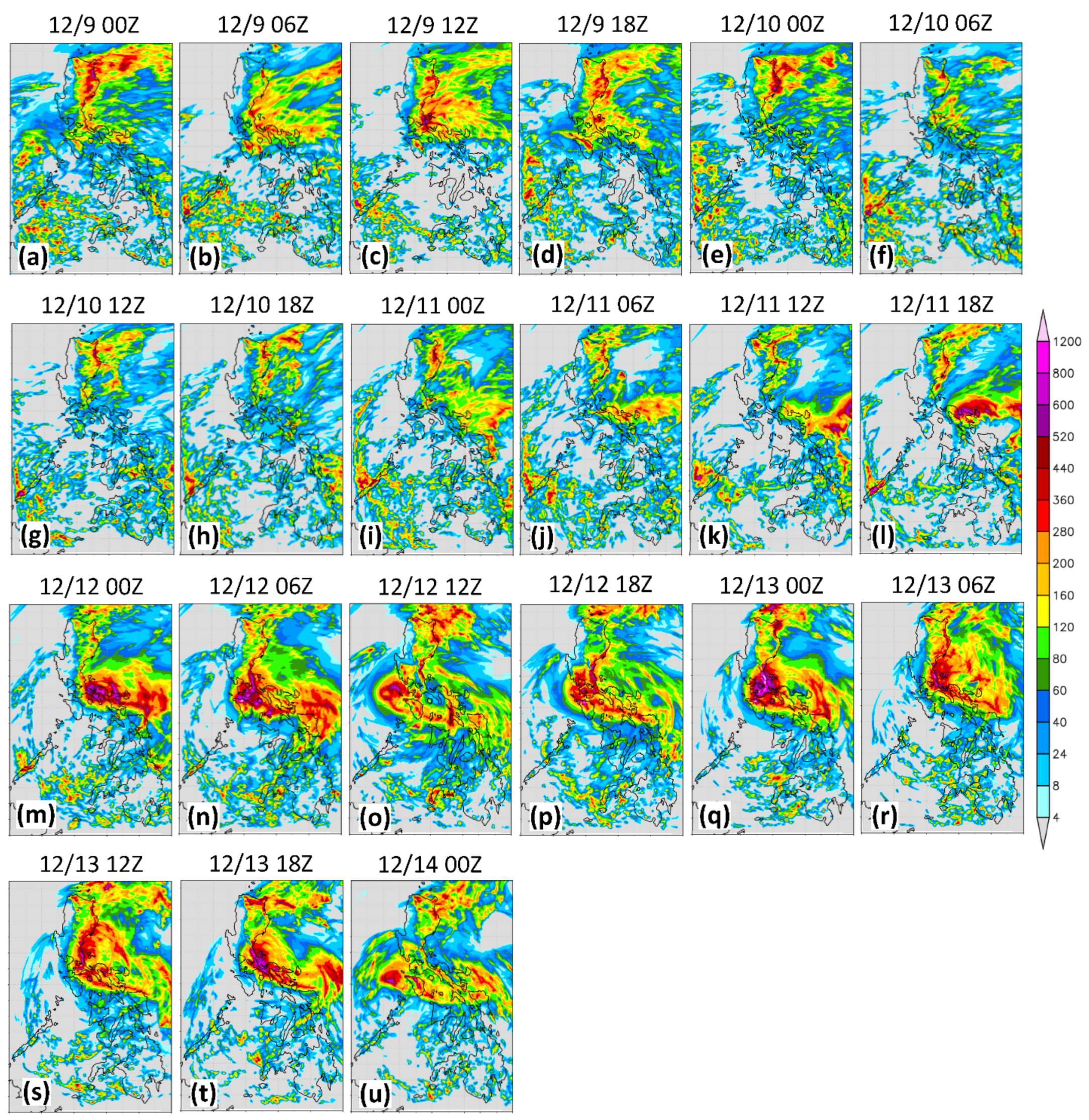
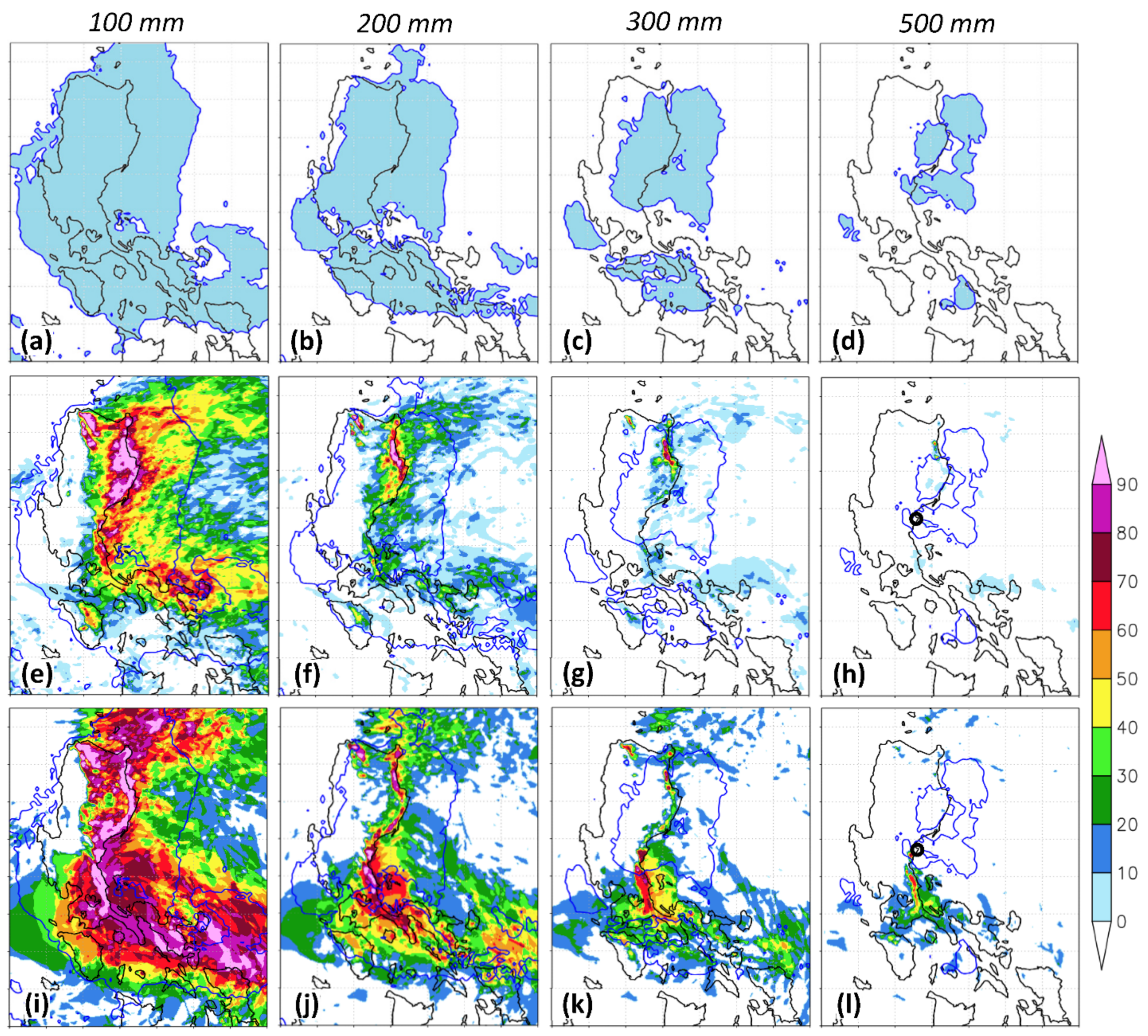
4.2. Observed and Predicted Rainfall of TY Koppu (2015)

Due to the slow translation speed of Koppu, the GPM retrievals showed different rainfall distributions day by day. From 1200 UTC on 16 to 1200 UTC on 17 October (Figure 9a), most rain was over the ocean east of central Luzon, with a peak amount of 950.4 mm. Over the second 24 h that covered the landfall period, the rain was over central and northern Luzon (north of approximately 15°N) and the peak was located in southern CCM (Figure 9b), again near Baguio. After 1200 UTC on 18 October, the 24 h rainfall was mostly near shore off north-western Luzon when the TC center exited the land, with a peak amount of 745.7 mm (Figure 9c). For the 72 h total, significant rainfall occurred in all three regions above, but the peak value was off the eastern coast of Luzon at 975.3 mm (Figure 9d). During each 24 h period, the middle part of the Philippine archipelago also received some rain in the GPM, but the local maxima were mostly below 100–150 mm.

As the convection was more active in the southern eyewall of Koppu, the QPFs over the whole period, by many lagged hindcasts, showed only one swath of maximum rainfall during the approach in Figure 10, and was in general agreement with Figure 9a. Due to the northward track bias, however, the position of this strip of higher rainfall was too far north in all the earlier runs (Figure 10a–j), and, apparently, became better only after 0600 UTC on 15 October (Figure 10k–o). In earlier runs, the peak value there could reach approximately 1000–1300 mm, and also exceeded the 975.3 mm in GPM data. Later, as the track improved, the peak value also became closer to the GPM value. For the rainfall over Luzon, not surprisingly, the northern part of the CCM and SMM received too much rain in the earlier runs with northward bias. With peak rainfall on land in the GPM (Figure 9d), the southern CCM also had plenty of rain in some earlier runs, and was in better agreement with the GPM perhaps since the run at 1200 UTC on 15 October (Figure 10). For the rain off western Luzon during and after landfall (mostly west of 119.5°E) in the GPM (Figure 9b–d), it was too close to land in most runs in Figure 10 due to the premature northward turn, except in the last 4–5 runs. In terms of amounts, the model seemed to predict too much rain over the CCM and SMM over land compared to the GPM, especially along the SMM, but was roughly on par for the offshore regions. Among all rain gauge sites (on land), again, the maximum was at Baguio at 695.3 mm and roughly 100 mm higher than the GPM. Therefore, the rainfall amounts over the mountain regions during Koppu might have been somewhat underestimated in the GPM as well.

4.3. Heavy Rainfall Probabilities of TY Koppu (2015)

The heavy-rainfall probabilities to reach 100, 200, 300, and 500 mm from the entire event of TY Koppu (2015) over 72 h (from 1200 UTC on 16 to 1200 UTC on 19 October), obtained from the first eight versus the last seven members are shown in Figure 11. At 100 and 200 mm (per 72 h), the areas of high probabilities from the first eight members (executed during 13–14 October), compared to the GPM (Figure 11a,b), were displaced north, mainly over the ocean, and did not extend east and south enough before landfall or west enough after landfall (Figure 11e,f) due to the larger track biases. Such a deficiency was alleviated at shorter lead times in the last seven runs, i.e., those from 0000 UTC on 15 to 1200 UTC on 16 October (Figure 11i,j). However, the high-probability region was still smaller than that in the GPM, as some northward bias before landfall and a premature northward turn over Luzon still existed (see Figure 2b). Over the ocean on both sides of Luzon, similar situations appeared in the probabilities of higher amounts of 300 and 500 mm, but the later members clearly improved and agreed better with the GPM (Figure 11c,d,g,h,k,l). On land, the probabilities of heavy rainfall at these two higher thresholds were again the highest over the CCM and SMM, and displaced northward in the early runs (Figure 11g,h). Not surprisingly, this error was corrected in the later runs, where the agreement at 300 mm with the GPM was particularly good in central Luzon (Figure 11k). In the GPM retrieval, a small area just east of Baguio reached 500 mm, while the 72 h accumulation measured with the rain gauge at Baguio recorded 695.3 mm [40], as mentioned. In the lagged runs, high probabilities at Baguio were also predicted, including in the earlier runs, despite their larger track biases (Figure 11h,l). Therefore, the lagged hindcasts during Koppu performed reasonably well in the probability estimates, especially with the later runs since 15 October. However, over the nearby ocean, the probability estimates (before and after landfall) were not as good due to track errors.

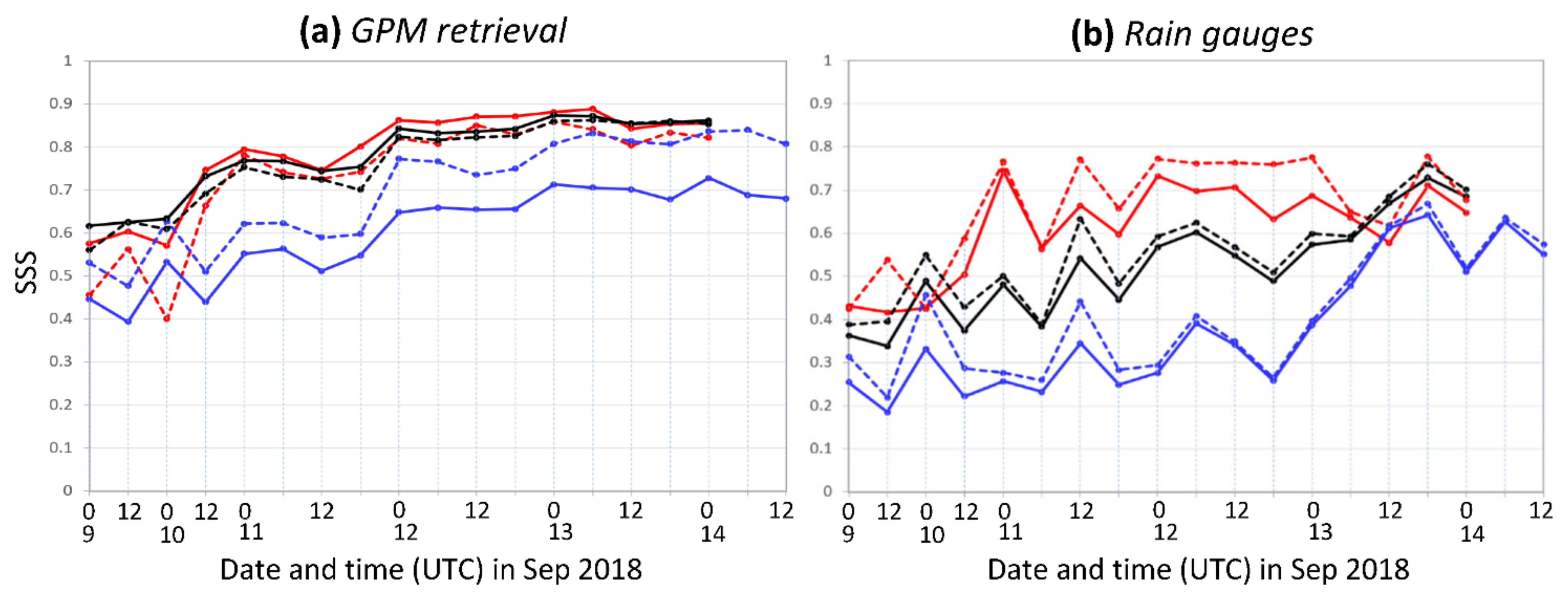
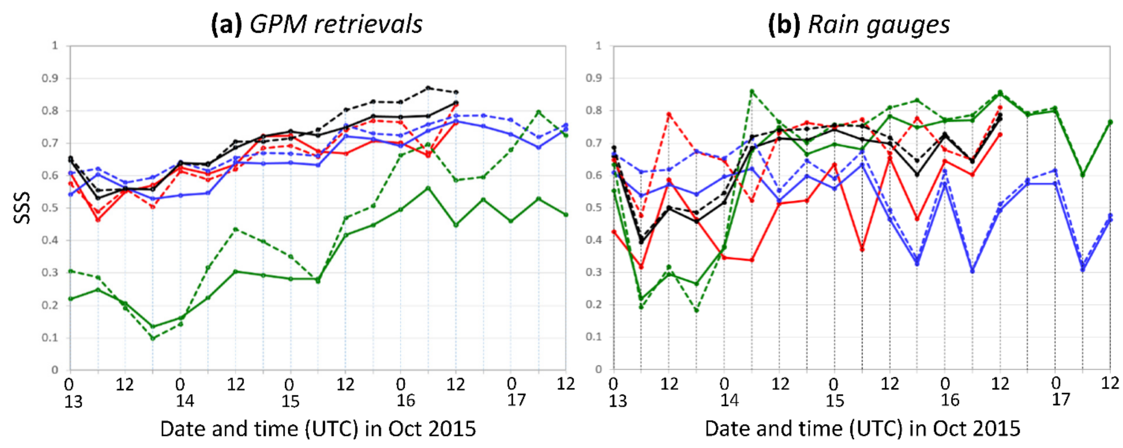
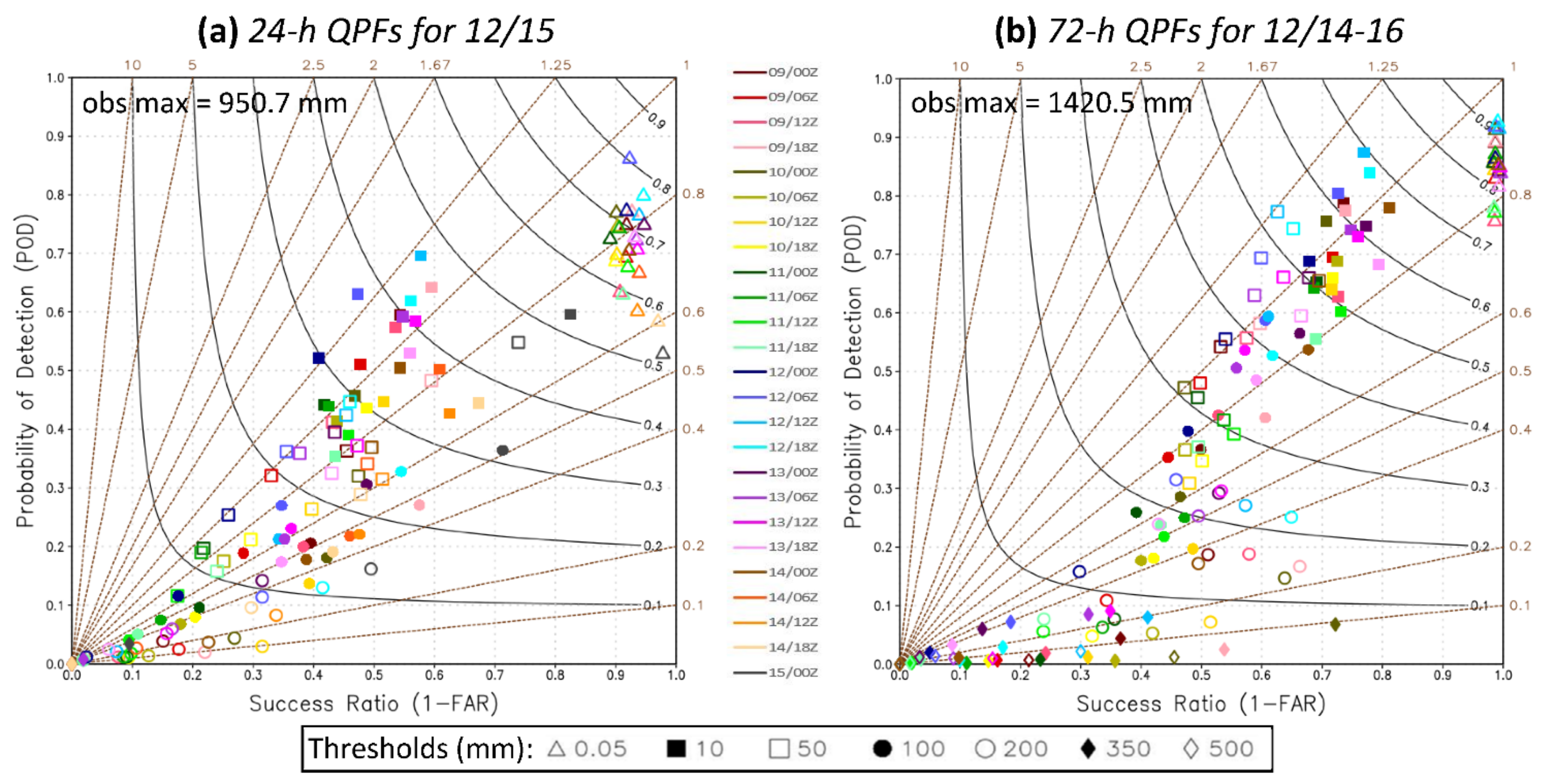
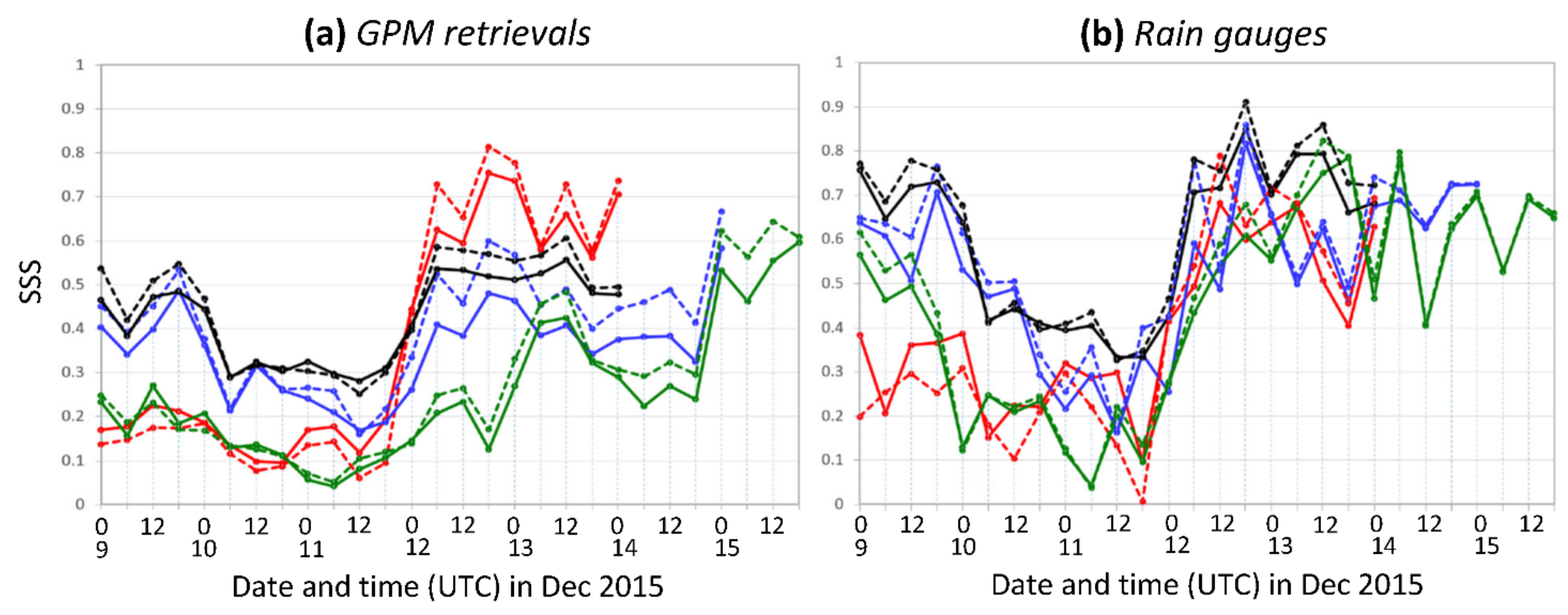
4.4. Objective Skill Scores of QPFs for TY Koppu (2015)

The categorical skill scores of the QPFs targeted for one 24 h and one 72 h period (entire event) for Koppu are plotted in Figure 12. The 24 h period chosen was from 1200 UTC on 17 to 1200 UTC on 18 October, again, because of there being more rainfall on land (Figure 9b), with a peak amount of 512.7 mm just east of Baguio. For this 24 h, the TSs were approximately 0.6–0.8 at 0.05 mm, over 0.48–0.7 at 50 mm, and mostly 0.1–0.31 at 200 mm, respectively (Figure 12a). Compared to those using rain gauges as the observation in Part I [40], i.e., their Figure 9b, the values here were considerably higher, both within the short range and beyond (except at 10 mm), particularly at 50 and 100 mm, as also summarized in

Table 3. As in Table 2, but for the comparison for TY Koppu (2015), in which the 24 h QPFs were for the second (1200 UTC on 17 to 1200 UTC on 18) and third (1200 UTC on 18 to 1200 UTC on 19) periods, and 72 h QPFs for 1200 UTC on 16 to 1200 UTC on 19 October 2015.

Koppu	Against GPM				Against Rain Gauges
24 h QPFs	Obs. Max.	Threshold (mm)			Obs. Max.	Threshold (mm)
Second period	(mm)	10	50	100	(mm)	10	50	100
t0 within 48 h (9)
Mean TS	512.7	0.54	0.54	0.42	188.8	0.53	0.24	0.11
Range of TS		0.07	0.14	0.08		0.20	0.12	0.18
t0 beyond 48 h (10)
Mean TS	512.7	0.50	0.60	0.47	188.8	0.47	0.29	0.18
Range of TS		0.12	0.16	0.18		0.08	0.13	0.15
24 h QPFs	Obs. Max.	Threshold (mm)			Obs. Max.	Threshold (mm)
Third period	(mm)	100	200	350	(mm)	100	200	350
t0 within 48 h (5)
Mean TS	400.0 #	0.26	0.10	0.01	502.3	0.36	0.28	0.40
Range of TS		0.10	0.06	0.04		0.14	0.50	1.00
t0 beyond 48 h (14)
Mean TS	400.0 #	0.16	0.05	0.00	502.3	0.21	0.24	0.46
Range of TS		0.21	0.14	0.04		0.32	0.50	1.00
72 h QPFs	Obs. Max.	Threshold (mm)			Obs. Max.	Threshold (mm)
	(mm)	200	350	500	(mm)	200	350	500
t0 within 48 h (9)
Mean TS	975.3	0.52	0.26	0.06	695.3	0.27	0.28	0.72
Range of TS		0.08	0.15	0.09		0.12	0.13	1.00
t0 beyond 48 h (6)
Mean TS	975.3	0.39	0.09	0.01	695.3	0.21	0.13	0.06
Range of TS		0.13	0.11	0.02		0.13	0.33	0.33

^# Estimated value inside the large domain from Figure 9c.

(top third). In Figure 12a, most TS values at 350 mm were also above zero and could be up to approximately 0.1, but this was not a valid threshold, since the maximum recorded with the gauges was only 188.8 mm at Baguio [40] (Table 3). In Figure 12a, the BS values indicated a slight underprediction (0.6 < BS < 0.8) at the lowest threshold of 0.05 mm and some overprediction (1.25 < BS ≤ 4) at the highest available threshold of 350 mm, but little tendency in between. On the contrary, the BSs of approximately 1–5 in Part I [40] suggested a strong overprediction, more serious toward the higher thresholds. This different result may have been somewhat expected, since the peak amount observed with the rain gauge network (over land only) was considerably lower than that in the GPM.

In Table 3, results for the third 24 h period (starting at 1200 UTC on 18 October) during Koppu were also compared because of their different characteristics. During this period, Baguio received 502.3 mm of heavy rainfall and the maximum value inside the large domain in the GPM was approximately 400 mm (Figure 9c). For this period, the TS results using the gauges were all higher than those against the GPM across the three available thresholds (100, 200, and 350 mm) in both forecast ranges, and more so at higher thresholds (Table 3, middle third). The former group (against the gauges) also exhibited greater ranges in values. Thus, for these two 24 h periods, distinctly different results were obtained using the two datasets. That is, due to there being much fewer verification points of the rain gauges (N = 56), the results in the categorical measures could be more unstable toward the higher thresholds, thus, could be much better or worse than the more stable results using the GPM IMERG data (N = 9916).

For the QPFs for the 72 h total rainfall from Koppu, the categorical scores are shown in Figure 12b, while the rainfall maximum in the GPM was 975.3 mm near 15°N 123°E (Figure 9d). The TSs were 0.76–0.88 at 0.05 mm (per 72 h), 0.52–0.65 at 100 mm, and from 0.05 to 0.35 at 350 mm, respectively (Figure 12b). At 500 mm, all the runs also registered nonzero TS values, and the highest one reached 0.11. Compared to the values in Part I [40], one could see that the scores using the GPM were considerably higher from 50 to 200 mm, and the two were comparable at low thresholds and at 350 mm (also Table 3, bottom third). However, almost all runs since 1200 UTC on 14 September in Part I [40] produced TSs of 1 or 0.5 at 500 mm when they captured the heavy rainfall at Baguio (peak amount = 693.5 mm in gauge observation). With a large number of verification points and more stable results, such high TS values at 500 mm using GPM data in Koppu (given the track errors) would not be possible here, as the hit rate was, at most, approximately 10% in the best member (see Figure 11h). In terms of the BS values, again, there was little bias in rain-area sizes in Figure 12b using the GPM data, but they indicated an overprediction in Part I [40]. Near Baguio, the GPM retrieval was approximately 700 mm, and was quite close to the rain gauge measurement, but the timing as derived from the satellites appeared to be shifted early (from after to before 1200 UTC on 18 October) when Figure 9 was compared with gauge measurements in Part I.

Figure 13 shows the results of the SSS for Koppu. First, for the 72 h total rainfall, the SSS values of the QPFs (between Figure 9d and Figure 10) over the large domain with the lagged runs increased gradually with time, from approximately 0.55–0.65 in the earlier runs to 0.83 in the last available run at 1200 UTC on 16 October (Figure 13a, solid black), which was in agreement with the track improvement and Figure 11. For the first 24 h period, when the main rainfall areas were east of Luzon (Figure 9a), the SSS values were slightly lower and also did not improve as much in the later runs (solid red). Similar SSS values were also obtained for the second 24 h period (1200 UTC on 17 to 1200 UTC on 18 October), when most of the rainfall on land occurred (in the GPM, Figure 9b), and the four latest runs became available with SSS values just below 0.8 (solid blue, Figure 13a). For these two 24 h periods, and also the 72 h period, the SSS values over the small domain (dashed) tended to be slightly higher than their counterparts over the entire Philippines, mostly by approximately 0.05 to 0.1. Note that the small domains were different for different 24 h periods (Figure 9). However, for the third 24 h period, the SSS values were much lower (solid green, Figure 13a) and only approximately 0.3 or below before t₀ = 1200 UTC on 15 October and approximately 0.4–0.56 afterwards (over the large domain). In general, the longer range of QPFs targeted at the last 24 h period could yield lowered SSS values in Figure 13a due to larger errors, compared to those targeted at earlier periods with the same runs. More specifically, the lowered scores were because the main rainfall areas already moved offshore during this period (see Figure 9c), but abundant rainfall occurred over Luzon due to the premature northward turn of the TC in the model, thus, producing a mismatch between the two patterns. Over the small domain that was moved farther west to include the main rainfall areas offshore (dashed green), the SSS was improved and could reach 0.7 in some runs (Figure 13a).

The above SSS curves were also compared with those obtained for the same domains but using the land-based rain gauge observations in Figure 13b, where the two curves for the 72 h QPFs were also shown in Part I [40]. The SSS results were seen to be less stable with more fluctuations up and down, and were, in general, lower for both the first and second 24 h periods (red and blue) and also the 72 h period (black), if the rain gauges were used. On the contrary, it was the opposite for the last 24 h period, as the hindcast at 1200 UTC on 14 and all those executed between 1200 UTC on 15 and 0000 UTC on 17 October could reach 0.75 against the gauge observations (green, Figure 13b). As discussed earlier, Baguio had 502 mm of rain on this day [40], but the GPM had only approximately 120 mm in Figure 9c, so the SSS could reach high values when the northward track bias became sufficiently small enough to allow for heavy rainfall near Baguio during the (premature) northward turn of Koppu in the model. Thus, the GPM seemed to underestimate the rainfall in southern CCM, potentially quite seriously. Additionally, for the rainfall on the third day, the SSS results over the small and large domains were often similar in Figure 13b (using the rain gauges), since the main rainfall area already moved offshore where there were no gauges.

5. Time-Lagged Ensemble QPFs for TY Melor (2015)

5.1. Track and Intensity of TY Melor (2015)

For Melor, which passed through central Philippines over 14–15 December 2015, a total of 28 hindcasts was determined. The runs during the first three days also had northward track biases during the approach (Figure 2c). For those during the first 24 h, however, the storm tracks turned south again and the errors reduced to ≤200 km toward the later stage of landfall, while those during the next two days moved too slowly even with a recovery, so track errors remained larger. The predicted tracks after 0000 UTC on 12 December improved, and their first landfall at Samar (approximately 0300 UTC on 14 December) was all inside 75 km from the best track (Figure 2c). After that, the model TCs moved through the archipelago during the next 1.5 days or so, as in the observation, and many had a track bias within 100 km at the time of exit. Overall, the track errors reduced to inside 75–80 km since the runs initialized approximately 66 h before the actual landfall for Mangkhut, approximately 59 h for Koppu, and approximately 45 h before the first landfall for Melor (Figure 2). The error of 75–80 km was comparable to averaged values at the lead time of 24 h [40], and, therefore, was considered very good when achieved at much longer lead times.

TY Melor (2015) reached its first landfall at northern Samar as a category four storm (Figure 1a). At this time, the minimum central MSLP was estimated to be near 934 hPa (Figure 3e). It then weakened somewhat before, finally, exiting Mindoro at approximately 953 hPa. The earlier runs before 1800 UTC on 11 December (those deviated northward) could not capture the rapid deepening over 12–13 December. While the intensity gradually improved, the hindcasts determined on 12 and 13 December could only produce a minimum MSLP of 952–963 hPa (except for the one at 1200 UTC on 13 December at t₀). Afterwards, the model storms could not deepen much from their initial MSLP of ≥972 hPa, as Melor was about to reach landfall, or already had (Figure 3e). Thus, the lagged runs could not fully capture the rapid intensification of Melor, whose central MSLP dropped by approximately 60 hPa in just 48 h. Similarly, for the maximum wind speed, estimated to be 62 m s⁻¹ by the JTWC near Melor’s first landfall (Figure 3f), the better members during 12–13 December could reach only approximately 50–54 m s⁻¹ (approximately 10 m s⁻¹ too low). Nonetheless, they exceeded the JMA estimate of 49 m s⁻¹. For the runs before 1800 UTC on 11 December and after 13 December, they could only reach approximately 40 m s⁻¹ at most (Figure 3f). Thus, deficits existed in the maximum wind speed for Melor, similar to the MSLP.

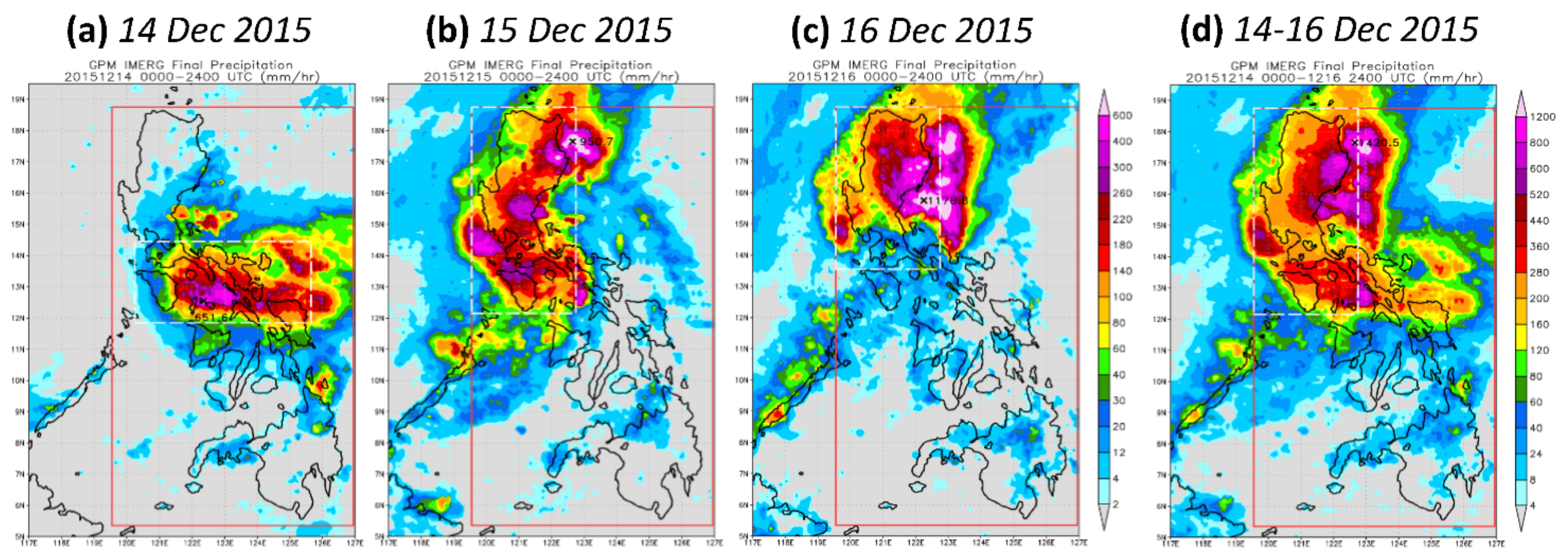
5.2. Observed and Predicted Rainfall of TY Melor (2015)

Although Melor moved through the Philippine archipelago at a moderate speed, it nearly stalled till 16 December after moving offshore (Figure 1a). Therefore, its impact duration was also quite long and, thus, three 24 h periods on 14–16 December were selected for examination. On the first day (14 December) that covered much of the landfall period, heavy rainfall occurred in central Philippines in the GPM data, including northern Samar, with a peak amount of 651.6 mm near 12.5°N, 122°E (Figure 14a). On 15 December, as Melor slowly moved across northern Mindoro (Figure 1a), significant rainfall was observed in northern Mindoro and nearby regions, and also near northeastern and central Luzon along the SMM, with a maximum of 950.7 mm near 17.5°N 123°E (Figure 14b). Along the SMM, localized rainfall also reached 600 mm on this day. On 16 December, as Melor stalled just west of Luzon, the most rainfall occurred in northeastern Luzon and the nearby ocean (Figure 14c), with a peak amount of 1178.8 mm approximately 80 km offshore, to the east of Baler (see Figure 1b for location). When summed over the three days, the peak rainfall amount in the GPM reached 1420.5 mm offshore near 17.5°N 123°E (Figure 14d), while the most rainfall on land was in northeastern to central Luzon, with over 800 mm along the SMM, followed by northern Mindoro, and the southernmost part of Luzon (approximately 300 mm).

In Part I [40], the maximum rainfall recorded with the rain gauges was 169.6 mm in central Philippines on 14, 209.2 mm in northern Mindoro on 15, and 273.8 mm at Baler to the east of SMM on 16 December, respectively. The maximum 72 h total over 14–16 December was 407 mm also at Baler [40]. In the GPM retrievals (Figure 14), the rainfall amounts at these locations were also comparable to the gauge data, although much higher amounts were indicated over the ocean. Along the SMM, over northeastern Luzon, the peak rainfall of >600 mm in Figure 14d could not be verified because of a lack of rain gauges in that region. However, at least on land, the GPM did not appear to overestimate or underestimate the total rainfall from Melor by much.

The QPFs for the 72 h rainfall over 14–16 December with the lagged runs are presented in Figure 15. Some of the earliest runs, as mentioned, exhibited relatively small track errors and, thus, could capture the abundant rainfall along the SSM and the eastern coast of Luzon, and even the rainfall in northern Mindoro (Figure 15a–e). However, in the next several runs (Figure 15f–k), the northward biases were larger and the landfall was delayed in the model, so the rainfall over northeastern Luzon also decreased. During 11 December (Figure 15i–l), the tracks gradually improved and some TCs could reach landfall over central Philippines (Figure 2c). After 0000 UTC on 12 December, the track forecasts further improved and a swath of more concentrated rainfall through central Philippines started to emerge in the predictions (Figure 15m–u), until the last available run at 0000 UTC on 14 December. Due to better tracks in these later runs, the predicted rainfall along the SSM in eastern Luzon also increased and could reach approximately 300–450 mm. In some runs, the rainfall in northern Mindoro was also captured, such as that initialized at 0600 and 1800 UTC on 12 (Figure 15n,p), and the two at 0000 UTC on 13 and 14 December (Figure 15q,u). However, most of the lagged runs predicted more rain along the SSM, but very few had comparable amounts over the offshore ocean, where the GPM data indicated much rainfall, except perhaps those from 0600 to 1800 UTC on 13 December (Figure 15r–t). Thus, a larger disagreement existed east of Luzon between the GPM and model predictions.

5.3. Heavy Rainfall Probabilities of TY Melor (2015)

In Figure 16, the probabilities of 72 h rainfall over 14–16 December to reach the four thresholds of 100, 200, 300, and 500 mm calculated from the first 12 runs versus the last nine runs for Melor are shown. The GPM data indicated that almost the entire northern half of the Philippines received a total rainfall of ≥100 mm (Figure 16a), including the entire Luzon island, the ocean within 150–200 km off its eastern shore, and regions from northern Samar to Mindoro. From the first 12 runs (with a t₀ up to 1800 UTC on 11 December), the highest probabilities to reach 100 mm appeared along the eastern shore and near the southeastern tip of Luzon, and also over Mindoro, but the probabilities were too low in western Luzon and the oceans in central Philippines (Figure 16e). In the last nine runs (Figure 16i), the low probabilities in central Philippines along the storm track were drastically improved due to the improvements in tracks, so were those in eastern Luzon and the offshore oceans. In western Luzon, however, the improvement seemed limited. At 200 mm, a smaller region reached this criterion in the GPM, but only slightly smaller (Figure 16b). In contrast, the probabilities from the lagged hindcasts reduced considerably almost everywhere. Due to the track errors, except along the SSM, the probabilities from the first 12 runs were too low over much of Luzon, its offshore ocean (to approximately 150 km), and central Philippines (Figure 16f). In the last nine members, the improvements were significant in central Philippines (from northern Samar to northern Mindoro) and along the eastern shore of Luzon, but not by much elsewhere (Figure 16j).

At 300 mm, the GPM (Figure 16c) still indicated a large area to meet this criterion, approximately 100 km both onshore and offshore of eastern Luzon from 15°N to 18°N, the ocean surrounded by southern Luzon and Mindoro, and an area west of Manila Bay, where Melor stalled. Except along a short segment of the SSM, the probabilities in the first 12 runs to reach 300 mm were all too low (Figure 16g). Again, the values were improved along the storm track and the SSM in the later members, including the area near Baler (Figure 16k). At 500 mm, the conditions were similar (Figure 16h,l). In the last nine runs, the probability to reach 500 mm was roughly 60–70% along the eastern coast of Luzon near Baler, where the gauge observed 407 mm. Overall, when the TC tracks were improved, the rainfall probabilities also improved quite significantly in central Philippines and along the SSM in eastern Luzon. In other regions, where the GPM also indicated heavy rainfall (>200 mm), however, the model seemed to underpredict rainfall and the improvement in probability in later runs appeared small.

5.4. Objective Skill Scores of QPFs for TY Melor (2015)

The categorical skill scores of the QPFs for the 24 h period on 15 December and the 72 h period of 14–16 December during Melor are shown in Figure 17. Here, 15 December was chosen because the rainfall on land was the most widespread among the three days (Figure 14b). In Figure 17a, the QPFs for 15 December with the lagged runs were seen to yield TSs of 0.52–0.8 at 0.05 mm (per 24 h) and from 0.05 to approximately 0.32 at 100 mm, respectively, while the observed peak amount was 950.7 mm in the GPM. At 200 mm, all the runs also produced nonzero TSs, which were maximized at 0.14, but the highest TS was only 0.03 at 350 mm. In Part I [40], the peak amount with the gauges was 209.2 mm in northern Mindoro, where the GPM captured approximately 260 mm, and was in reasonable agreement. As shown in

Table 4. As in Table 2, but for the comparison of TY Melor (2015), in which the 24 h QPFs are for 15 December and 72 h QPFs for 14–16 December 2015 (all in UTC).

Melor	Against GPM				Against Rain Gauges
24 h QPFs	Obs. Max.	Threshold (mm)			Obs. Max.	Threshold (mm)
	(mm)	50	100	200	(mm)	50	100	200
t0 within 48 h (9)
Mean TS	950.7	0.18	0.06	0.00	209.2	0.46	0.3	0.12
Range of TS		0.19	0.12	0.03		0.29	0.39	1.00
t0 beyond 48 h (16)
Mean TS	950.7	0.12	0.03	0.00	209.2	0.24	0.10	0.03
Range of TS		0.23	0.10	0.00		0.36	0.67	0.33
72 h QPFs	Obs. Max.	Threshold (mm)			Obs. Max.	Threshold (mm)
	(mm)	100	200	350	(mm)	100	200	350
t0 within 48 h (9)
Mean TS	1420.5	0.39	0.20	0.04	407	0.48	0.32	0.08
Range of TS		0.16	0.12	0.07		0.35	0.58	0.33
t0 beyond 48 h (12)
Mean TS	1420.5	0.21	0.09	0.02	407	0.22	0.11	0.00
Range of TS		0.19	0.12	0.06		0.32	0.31	0.00

(top half), the TSs obtained using the gauges were all better across the three thresholds of 50, 100, and 200 mm compared to those using the GPM at both the short range and beyond, even though they were also less stable with larger ranges. In Figure 17a, the points also indicated some underprediction at the lowest threshold of 0.05 mm (BSs approximately 0.6–0.9) and higher thresholds of 100 mm (BSs approximately 0.4–0.8) and above (BS ≤ 0.5 mostly), while little bias to a slight overprediction existed at 10 and 50 mm.

Over 14–16 December, the peak amount with the gauges was 407 mm at Baler in Part I [40]. The GPM estimated a very high value of 1420.5 mm offshore of northeastern Luzon, but approximately 500 mm near Baler, also only somewhat higher than the gauge record. Therefore, the GPM appeared reasonable during Melor, but some past studies suggested caution in their extreme values, e.g., the top 1% [60]. The categorical scores for the 3-day total rainfall against the GPM were plotted in Figure 17b. The TSs were 0.75–0.92 at 0.05 mm (per 72 h) and decreased to approximately 0.05 to 0.24 at 200 mm. At 350 mm, all runs produced TSs above zero (up to 0.08), while 9 out of 21 runs also yielded TS > 0, but only up to 0.02. These TS values from 100 to 350 mm in Figure 17b were somewhat worse than their counterparts using the gauge data at the short range (where high TS values could appear occasionally), but roughly comparable at longer ranges (Table 4, bottom half). In Figure 17b, the BSs, again, suggested an underprediction at thresholds beyond 100 mm, especially at 350 and 500 mm (with BSs mostly below 0.5). This result was consistent with the low heavy rainfall probabilities over Luzon and the offshore ocean to the east in Figure 16. In Part I [40], the verification using rain gauges also indicated underforecasting.

In terms of the SSS, the values for 14 December for the large domain from the earlier runs at longer lead times were quite low at approximately 0.1–0.2 (solid red, Figure 18a), as the northward track errors could not be reduced in time. However, since 0600 UTC on 12 December, all the runs yielded an SSS of at least approximately 0.6 as the TC tracks improved. For 15 December, the runs on 9 December (solid blue, Figure 18a) could produce better SSS values (approximately 0.4–0.5) when the storm turned south again, but the later members also had approximately 0.4–0.6, clearly due to the underprediction of rainfall over eastern Luzon and offshore against the GPM (see Figure 16 and Figure 17a). For 16 December, the SSS values from runs before 0000 UTC on 13 December were also low and below 0.25 (solid green), and improved to approximately 0.5–0.6 only in the last several runs on 15 December. For the 72 h QPFs for 14–16 December, the earlier runs on 9 December could also achieve SSS values of 0.4–0.5, followed by less ideal results, then improved to 0.5 and above since 0600 UTC on 12 December (solid black, Figure 18a), in agreement with Figure 14, Figure 15, Figure 16 and Figure 17. Over the small domain, which had an east–west orientation for 14 December (see Figure 14), the SSS values tended to be slightly higher than those over the large domain, but this was not always the case (dashed curves, Figure 18a).

For comparison, the SSS results against the rain gauge observations are shown in Figure 18b, in which the two curves for the 72 h QPFs were shown in Part I [40]. Again, the values using the rain gauge data were less stable and spanned a wider range, with a lower minimum (nearly zero) and a higher maximum (>0.9). However, in most runs, the values in Figure 18b were higher than those using the GPM data, especially for those during the first day (on 9 December) and since 0600 UTC on 12 December, in contrast to the results shown in Figure 8 and Figure 13 for Mangkhut and Koppu. Nevertheless, such a result for Melor was in agreement with the underprediction in rainfall over the ocean east of Luzon. Thus, using the GPM data, which included the ocean, the resulting SSS values tended to be lower for Melor.

6. Discussion

In previous sections, the QPF verification results for the three typhoons were seen to be different to some extent when two different data sources were used: the GPM IMERG retrievals and rain gauge data. Here, such differences were further discussed. In Section 3, Section 4 and Section 5, Table 2, Table 3 and Table 4 were used to compare the TS values for selected target periods for the three TCs, and they indicated that the TSs were much more stable using the high-resolution GPM data compared to the rain gauges (which were much fewer in number), especially at lower thresholds, over longer accumulation periods, and in earlier forecasts with longer lead times. On the other hand, toward the high thresholds, where the TSs against the GPM inevitably dropped, the results using the rain gauges (more random) could become much better, particularly within the short range when the track errors became small. Presumably mainly due to the difference in the density and number of points available for verification, this phenomenon of diverging verification results clearly occurred in both Koppu (also beyond the short range) and Melor (≥50–100 mm), and also in Mangkhut (≥100 mm for 15 September), to a lesser degree.

As for the reliability of the GPM data in the three TC cases, the overall quality seemed reasonable. However, the satellite retrievals were likely to underestimate the rainfall from Mangkhut in the mountain regions (CCM and SMM) in Luzon, where some timing issues (too early) also existed during Koppu. For Melor, the estimates on land seemed reasonable, but the values offshore were very high and could potentially exhibit overestimation, which could not be confirmed. Based on the categorical verification results using the GPM IMERG data only, the QPF performance was the best for Koppu, followed by Mangkhut, and the worst for Melor, while the differences among cases were not too large due to the more stable results. In Part I [40], the order was not the same in Koppu, Melor, and Mangkhut. However, Koppu remained the most predictable among the three events.

Thus, based on our results here, we suggest that the GPM data were, in general, reasonable and suitable for the verification of QPFs with NWP models using the categorical measures, even on a routine basis in the long run. However, toward the high and extreme thresholds, if they revealed different results, station data from rain gauges (although few in number) would still be necessary to provide a second verification. This was especially true near and over the mountains, where satellite estimates could possess larger errors, such as Baguio (in the southwestern CCM) and Baler (along the SMM) in Luzon.

Compared to categorical scores, the SSS was not so sensitive to the number of verification points, as all points with rainfall were involved in the calculation, rather than only those reaching a given threshold. Additionally, hits were not required, so the same differences below or above the observed amount contributed almost the same, in contrast to the situation of categorical measures for over- (hits) or underprediction (no hits). In

Table 5. Comparison of mean, median, and range of SSS values with the CReSS hindcasts for the three typhoons against the GPM retrievals (left) and the rain gauges (right) in each category: 24 h QPFs over small domains for selected periods of P1, P2, and P3 (top) and 48 h or 72 h QPFs for entire events over the large domain (bottom), within the short range (t₀ ≤ 48 h before the beginning of accumulation) and beyond. All the periods shown are the same as those in Section 4, Section 5 and Section 6, and the number of lagged runs is given in the parentheses. Bold faces indicate the better result between the two data sources (higher mean/median but smaller range).

Forecast Range	Against GPM				Against Rain Gauges
24 h QPFs	Obs. Max.	SSS values			Obs. Max.	SSS values
Typhoon/period	(mm)	Mean	Median	Range	(mm)	Mean	Median	Range
t0 within 48 h
Mangkhut, P1 (9)	451.5	0.830	0.820	0.055	209.2	0.728	0.762	0.160
Mangkhut, P2 (7)	337.9	0.821	0.813	0.033	535.6	0.558	0.574	0.273
Koppu, P1 (9)	950.4	0.713	0.692	0.201	109.6	0.733	0.712	0.162
Koppu, P2 (9)	512.7	0.754	0.756	0.067	188.8	0.474	0.493	0.311
Koppu, P3 (5)	400.0 #	0.676	0.679	0.209	502.3	0.767	0.792	0.254
Melor, P1 (9)	651.6	0.671	0.728	0.380	169.6	0.612	0.631	0.367
Melor, P2 (9)	950.7	0.488	0.461	0.265	209.2	0.649	0.657	0.248
Melor, P3 (8)	1178.8	0.457	0.444	0.352	273.8	0.618	0.647	0.388
t0 beyond 48 h
Mangkhut, P1 (8)	451.5	0.634	0.695	0.382	209.2	0.591	0.575	0.346
Mangkhut, P2 (12)	337.9	0.634	0.622	0.296	535.6	0.321	0.291	0.237
Koppu, P1 (6)	950.4	0.555	0.567	0.124	109.6	0.626	0.647	0.313
Koppu, P2 (10)	512.7	0.631	0.631	0.091	188.8	0.641	0.649	0.162
Koppu, P3 (14)	400.0 #	0.367	0.334	0.597	502.3	0.625	0.756	0.678
Melor, P1 (12)	651.6	0.128	0.136	0.125	169.6	0.208	0.215	0.303
Melor, P2 (16)	950.7	0.364	0.356	0.441	209.2	0.523	0.517	0.696
Melor, P3 (20)	1178.8	0.207	0.171	0.432	273.8	0.419	0.451	0.787
48/72 h QPFs	Obs. Max.	SSS values			Obs. Max.	SSS values
Typhoon	(mm)	Mean	Median	Range	(mm)	Mean	Median	Range
t0 within 48 h
Mangkhut (9)	455.2	0.852	0.855	0.042	785.8	0.605	0.585	0.240
Koppu (9)	975.3	0.754	0.749	0.138	695.3	0.702	0.712	0.171
Melor (9)	1420.5	0.505	0.519	0.151	407.0	0.703	0.706	0.424
t0 beyond 48 h
Mangkhut (8)	455.2	0.705	0.738	0.152	785.8	0.427	0.364	0.204
Koppu (6)	975.3	0.595	0.599	0.117	695.3	0.535	0.507	0.292
Melor (12)	1420.5	0.365	0.325	0.204	407.0	0.519	0.429	0.423

^# Estimated value inside the large domain from Figure 9c (as in Table 3).

, a comparison in the SSS is given. For 24 h QPFs (over small domains), the two methods were quite comparable inside the short range (Table 5, top), with better SSS values from the GPM data for Mangkhut, but not so much for the majority of periods for Koppu and Melor. However, the GPM did tend to produce smaller ranges in the SSS due to larger numbers of points (see Figure 4, Figure 9 and Figure 14). At longer ranges (Table 5, middle), the GPM again yielded better SSS values for Mangkhut, but the opposite for both Koppu and Melor (mostly due to the model’s ability to capture heavy rainfall near Baguio). For QPFs for the entire events (48 or 72 h), SSS values (over the large domain) using the GPM were clearly better at both forecast ranges for Mangkhut and Koppu, but not so much for Melor (Table 5, bottom). Compared to the other two TCs, the differences for Koppu were relatively small. Overall, the SSS values computed using GPM data were highest for Mangkhut, followed by Koppu, and lowest for Melor (Table 5, left half). As a skill score, the SSS could faithfully reflect the overall quality of the QPFs over the verification domain in an objective and quantitative manner, but except that, the errors were squared (using MSE); this did not emphasize high rainfall amounts.

7. Conclusions

In this two-part study, the 2.5 km CReSS was applied to three landfalling typhoons in the Philippines: Mangkhut (2018), Koppu (2015), and Melor (2015), using the time-lagged approach every 6 h to form an ensemble. The single-model lagged method was adopted to achieve a high resolution, and, eventually, the multimember ensemble with the same resolution would be desired when more computation resources become available, e.g., [77,78]. The three westward-moving typhoons reached landfall in northern Luzon, central Luzon, and the middle part of the entire Philippine archipelago, respectively. Using categorical scores and the SSS, the QPFs were evaluated at 56 rain gauge sites in Part I [40] and, subsequently, using 0.1° × 0.1° high-resolution GPM IMERG rainfall retrievals in the same way in the present work. The verification results were compared and the quality of the GPM data was also assessed. In this study, the intensity forecasts and heavy-rainfall probabilities derived from successive lagged members at different lead-time groups were also evaluated. The major findings were summarized below.

Over the large domain that covers the entire Philippines (including nearby oceans) with 9916 grid points, the general quality of the GPM data during the three TCs was reasonable. However, an underestimation likely occurred in the mountain regions of Luzon during Mangkhut, and some timing issues also appeared during Koppu. For Melor, the peak amount offshore (over 1400 mm in 72 h) seemed excessive and potentially overestimated. Based on the categorical statistics against the GPM, the model QPFs performed the best for Koppu, followed by Mangkhut, and the worst for Melor. This order of predictability was different (switched) between Mangkhut and Melor from Part I [40], but Koppu remained the most predictable case in rainfall.

For TY Koppu (2015), the 24 h period selected for verification was 1200 UTC on 17 to 1200 UTC on 18 October (peak = 512.7 mm at southern CCM), and the lagged runs at the short range (entire verification period was within 72 h from t₀) produced mean TSs of 0.24 and 0.05 at 200 and 350 mm (per 24 h) against the GPM, respectively. At lead times, beyond the short range, the mean TSs at the same thresholds were 0.12 and 0.01. For the entire 72 h event (1200 UTC on 16 to 1200 UTC on 19 October), the maximum rainfall in the GPM was 975.3 mm (over ocean), and the short-range runs produced mean TSs of 0.52 and 0.06 at 200 and 500 mm (per 72 h), respectively. Beyond the short range, the mean TSs at 200 mm were 0.39. The BS values for Koppu generally showed little biases in rain-area sizes. At both short range and beyond, the majority of runs (>90%) produced rainfall of ≥500 mm near Baguio in the southern CCM, with high probabilities of heavy rainfall. The intensity forecasts were also the best for Koppu (926 hPa and 66.5 m s⁻¹ in JTWC’s best track) among the three cases, as many short-range runs reached ≤920 hPa and ≥60 m s⁻¹.

For TY Mangkhut (2018), which hit the northernmost part of Luzon, the most rainy 24 h on land was 15 September, with a peak rainfall of 337.9 mm in the southern CCM in the GPM. For this period, the mean TSs were 0.39 and 0.12 at 100 and 200 mm (per 24 h) inside the short range and 0.22 and 0.04 at longer lead times, respectively. For the two-day total rainfall (14–15 September, peak amount = 455.2 mm offshore), the mean TSs reached 0.36 at 200 mm and 0.02 at 350 mm (per 48 h) at the short range. Beyond the short range, the mean TSs were 0.18 and 0.01 at the same thresholds, respectively. The BSs indicated little bias at low to middle thresholds and some overprediction at high thresholds. Due to a reduction in track errors, the probabilities of heavy rainfall at 300 and 500 mm improved considerably from longer lead times to within the short range, as well as in the mean TS and SSS values (from 0.71 to 0.85). As the most intense (category five) storm before landfall among the three cases (905 hPa and 72 m s⁻¹), Mangkhut was also well captured in its intensity with the lagged runs, as many runs produced ≤900 hPa and at least 60 m s⁻¹.

For TY Melor (2015), which penetrated the middle section of the Philippine archipelago, the 24 h period selected was 15 December, when the maximum rainfall in the GPM reached 950.7 mm offshore and approximately 600 mm along the SSM on land. The mean TSs for this period were only 0.06 and 0.03 at 100 mm (per 24 h) inside the short range and beyond. For the three-day total rainfall (peak = 1420.5 mm offshore and over 800 mm in the SMM), the mean TSs at 200 and 350 mm (per 72 h) from short-range runs were 0.20 and 0.04, respectively. At longer lead times, the mean TSs at 200 mm were 0.09. The BSs for Melor suggested an underprediction toward the higher thresholds, especially for the three-day total, consistent with the relatively low TSs and the derived probabilities. Even at short range (for the first 24 h of the total period), roughly 60–70% of runs produced rainfall over 300 mm and 30–50% reached ≥500 mm along the southern SMM. For Melor (933 hPa and 62 m s⁻¹), the intensity forecasts were also less ideal, as only six to seven runs in the middle of the whole ensemble reached ≤960 hPa and ≥50 m s⁻¹.

Compared to the categorical statistics against the rain gauge observations in Part I [40], the results against the GPM IMERG retrievals were much more stable, especially at lower thresholds, over longer accumulation periods, and in earlier forecasts at longer lead times. However, due to the large number of points, the TSs inevitably dropped toward the high thresholds using the GPM data. In such circumstances, the results using the rain gauges could become much better, particularly within the short range when track errors became small. Such diverging verification results occurred in both Koppu and Melor, and also in Mangkhut, to a lesser degree. In terms of the BS values, the two data sources may have also given somewhat different results, but those using the GPM should have been more reliable.

Therefore, based on our results, it is suggested that the GPM is, in general, suitable for the verification of model QPFs using categorical measures, even routinely in the long-term. Over ocean and data-sparse regions, such satellite products may be the only data source available and robust enough for rainfall. However, toward higher and extreme thresholds, rain gauge observations are still needed to provide additional assessments of model performance, if they reveal different results. This is especially true near and over mountains, such as the CCM and SMM in Luzon, since satellite estimates may have larger errors there. As for the SSS, it could faithfully reflect the overall quality of the QPFs, but it did not focus on high rainfall thresholds.

References

1. Brown, S. The Philippines is the most storm-exposed country on Earth. Time, 11 November 2013. [Google Scholar]
2. Wannewitz, S.; Hagenlocher, M.; Garschagen, M. Development and validation of a sub-national multi-hazard risk index for the Philippines. GI_Forum 2016, 1, 133–140. [Google Scholar] [CrossRef] [Green Version]
3. Cinco, T.A.; de Guzman, R.G.; Ortiz, A.M.D.; Delfino, R.J.P.; Lasco, R.D.; Hilario, F.D.; Juanillo, E.L.; Barba, R.; Ares, E.D. Observed trends and impacts of tropical cyclones in the Philippines. Int. J. Climatol. 2016, 36, 4638–4650. [Google Scholar] [CrossRef] [Green Version]
4. Guha-Sapir, D.; Hoyois, P.; Wallemacq, P.; Below, P. Annual Disaster Statistical Review 2016. The Numbers and Trends; Centre for Research on the Epidemiology of Disasters (CRED), Institute of Health and Society (IRSS), and Université Catholique de Louvain: Brussels, Belgium, 2017; 80p, Available online: https://www.emdat.be/sites/default/files/adsr_2016.pdf (accessed on 20 June 2022).
5. NDRRMC (National Disaster Risk Reduction and Management Council). Effects of Typhoon “Yolanda” (Haiyan). SitRep. 108; NDRRMCL: Quezon City, Philippines, 2014; 67p. Available online: https://www.ndrrmc.gov.ph/attachments/article/1329/Effects_of_Typhoon_YOLANDA_(HAIYAN)_SitRep_No_108_03APR2014.pdf (accessed on 7 April 2020).
6. Soria, J.L.A.; Switzer, A.D.; Villanoy, C.L.; Fritz, H.M.; Bilgera, P.H.T.; Cabrera, O.C.; Siringan, F.P.; Maria, Y.Y.S.; Ramos, R.D.; Fernandez, I.Q. Repeat storm surge disasters of Typhoon Haiyan and its 1897 predecessor in the Philippines. Bull. Am. Meteorol. Soc. 2016, 97, 31–48. [Google Scholar] [CrossRef]
7. Wang, C.-C.; Lee, C.-Y.; Jou, B.J.-D.; Celebre, C.P.; David, S.; Tsuboki, K. High-resolution time-lagged ensemble prediction for landfall intensity of Super Typhoon Haiyan (2013) using a cloud-resolving model. Weather Clim. Extrem. 2022, 37, 100473. [Google Scholar] [CrossRef]
8. Golding, B.W. Quantitative precipitation forecasting in the UK. J. Hydrol. 2000, 239, 286–305. [Google Scholar] [CrossRef]
9. Fritsch, J.M.; Carbone, R.E. Improving quantitative precipitation forecasts in the warm season. A USWRP research and development strategy. Bull. Am. Meteorol. Soc. 2004, 85, 955–965. [Google Scholar] [CrossRef] [Green Version]
10. Czajkowski, J.; Villarini, G.; Michel-Kerjan, E.; Smith, J.A. Determining tropical cyclone inland flooding loss on a large scale through a new flood peak ratio-based methodology. Environ. Res. Lett. 2013, 8, 044056. [Google Scholar] [CrossRef]
11. Opiso, E.M.; Puno, G.R.; Alburo, J.L.P.; Detalla, A.L. Landslide susceptibility mapping using GIS and FR method along the Cagayan de Oro-Bukidnon-Davao City route corridor, Philippines. KSCE J. Civ. Eng. 2016, 20, 2506–2512. [Google Scholar] [CrossRef]
12. Cabrera, J.S.; Lee, H.S. Flood risk assessment for Davao Oriental in the Philippines using geographic information system-based multi-criteria analysis and the maximum entropy model. J. Flood Risk Manag. 2020, 13, e12607. [Google Scholar] [CrossRef] [Green Version]
13. Cuo, L.; Pagano, T.C.; Wang, Q.J. A review of quantitative precipitation forecasts and their use in short- to medium-range streamflow forecasting. J. Hydormeteorol. 2011, 12, 713–728. [Google Scholar] [CrossRef]
14. Kneis, D.; Abona, C.; Bronsterta, A.; Heistermanna, M. Verification of short-term runoff forecasts for a small Philippine basin (Marikina). Hydrol. Sci. J. 2017, 62, 205–216. [Google Scholar] [CrossRef]
15. MacLeod, D.; Easton-Calabria, E.; de Perez, E.C.; Jaime, C. Verification of forecasts for extreme rainfall, tropical cyclones, flood and storm surge over Myanmar and the Philippines. Weather Clim. Extrem. 2021, 33, 100325. [Google Scholar] [CrossRef]
16. Yeh, T.-C.; Cayanan, E.O.; Hsiao, L.-F.; Chen, D.-S.; Tsai, Y.-T. A study of the rainfall and structural changes of Typhoon Koppu (2015) over northern Philippines. Terr. Atmos. Ocean. Sci. 2021, 32, 619–632. [Google Scholar] [CrossRef]
17. Chang, C.-P.; Yeh, T.-C.; Chen, J.-M. Effects of terrain on the surface structure of typhoons over Taiwan. Mon. Weather Rev. 1993, 121, 734–752. [Google Scholar] [CrossRef]
18. Cheung, K.K.W.; Huang, L.-R.; Lee, C.-S. Characteristics of rainfall during tropical cyclone periods in Taiwan. Nat. Hazards Earth Syst. Sci. 2008, 8, 1463–1474. [Google Scholar] [CrossRef]
19. Su, S.-H.; Kuo, H.-C.; Hsu, L.-H.; Yang, Y.-T. Temporal and spatial characteristics of typhoon extreme rainfall in Taiwan. J. Meteorol. Soc. Jpn. 2012, 90, 721–736. [Google Scholar] [CrossRef] [Green Version]
20. Lee, C.-S.; Huang, L.-R.; Shen, H.-S.; Wang, S.-T. A climatology model for forecasting typhoon rainfall in Taiwan. Nat. Hazards 2006, 37, 87–105. [Google Scholar] [CrossRef]
21. Lee, C.-S.; Huang, L.-R.; Chen, D.Y.-C. The modification of the typhoon rainfall climatology model in Taiwan. Nat. Hazards Earth Syst. Sci. 2013, 13, 65–74. [Google Scholar] [CrossRef]
22. Hong, J.-S.; Fong, C.-T.; Hsiao, L.-F.; Yu, Y.-C.; Tzeng, C.-Y. Ensemble typhoon quantitative precipitation forecasts model in Taiwan. Weather Forecast. 2015, 30, 217–237. [Google Scholar] [CrossRef]
23. Wang, C.-C. The more rain, the better the model performs—The dependency of quantitative precipitation forecast skill on rainfall amount for typhoons in Taiwan. Mon. Weather Rev. 2015, 143, 1723–1748. [Google Scholar] [CrossRef]
24. Wang, C.-C.; Chang, C.-S.; Wang, Y.-W.; Huang, C.-C.; Wang, S.-C.; Chen, Y.-S.; Tsuboki, K.; Huang, S.-Y.; Chen, S.-H.; Chuang, P.-Y.; et al. Evaluating quantitative precipitation forecasts using the 2.5 km CReSS model for typhoons in Taiwan: An update through the 2015 season. Atmosphere 2021, 12, 1501. [Google Scholar] [CrossRef]
25. Wang, C.-C.; Paul, S.; Huang, S.-Y.; Wang, Y.-W.; Tsuboki, K.; Lee, D.-I.; Lee, J.-S. Typhoon quantitative precipitation forecasts by the 2.5 km CReSS model in Taiwan: Examples and role of topography. Atmosphere 2022, 13, 623. [Google Scholar] [CrossRef]
26. Gentry, M.S.; Lackmann, G.M. Sensitivity of simulated tropical cyclone structure and intensity to horizontal resolution. Mon. Weather Rev. 2010, 138, 688–704. [Google Scholar] [CrossRef] [Green Version]
27. Hoffman, R.N.; Kalnay, E. Lagged average forecasting, an alternative to Monte Carlo forecasting. Tellus A 1983, 35, 100–118. [Google Scholar] [CrossRef]
28. Wang, C.-C.; Huang, S.-Y.; Chen, S.-H.; Chang, C.-S.; Tsuboki, K. Cloud-resolving typhoon rainfall ensemble forecasts for Taiwan with large domain and extended range through time-lagged approach. Weather Forecast. 2016, 31, 151–172. [Google Scholar] [CrossRef]
29. Lorenz, E.N. Deterministic nonperiodic flow. J. Atmos. Sci. 1963, 20, 130–141. [Google Scholar] [CrossRef]
30. Epstein, E.S. Stochastic dynamic prediction. Tellus 1969, 21, 739–759. [Google Scholar] [CrossRef]
31. Toth, Z.; Kalnay, E. Ensemble forecasting at NMC: The generation of perturbations. Bull. Am. Meteorol. Soc. 1993, 74, 2317–2330. [Google Scholar] [CrossRef]
32. Molteni, F.; Buizza, R.; Palmer, T.N.; Petroliagis, T. The ECMWF Ensemble Prediction System: Methodology and validation. Q. J. R. Meteorol. Soc. 1996, 122, 73–119. [Google Scholar] [CrossRef]
33. Roebber, P.J.; Schultz, D.M.; Colle, B.A.; Stensrud, D.J. Toward improved prediction: High-resolution and ensemble modeling systems in operations. Weather Forecast. 2004, 19, 936–949. [Google Scholar] [CrossRef]
34. Mittermaier, M.P. Improving short-range high-resolution model precipitation forecast skill using time-lagged ensembles. Q. J. R. Meteorol. Soc. 2007, 133, 1487–1500. [Google Scholar] [CrossRef]
35. Lu, C.; Yuan, H.; Schwartz, B.E.; Benjamin, S.G. Short-range numerical weather prediction using time-lagged ensembles. Weather Forecast. 2007, 22, 580–595. [Google Scholar] [CrossRef]
36. Yuan, H.; McGinley, J.A.; Schultz, P.J.; Anderson, C.J.; Lu, C. Short-range precipitation forecasts from time-lagged multimodel ensembles during the HMT-West-2006 campaign. J. Hydrometeorol. 2008, 9, 477–491. [Google Scholar] [CrossRef]
37. Trilaksono, N.J.; Otsuka, S.; Yoden, S. A time-lagged ensemble simulation on the modulation of precipitation over West Java in January–February 2007. Mon. Weather Rev. 2012, 140, 601–616. [Google Scholar] [CrossRef] [Green Version]
38. Wang, C.-C.; Chen, S.-H.; Tsuboki, K.; Huang, S.-Y.; Chang, C.-S. Application of time-lagged ensemble quantitative precipitation forecasts for Typhoon Morakot (2009) in Taiwan by a cloud-resolving model. Atmosphere 2022, 13, 585. [Google Scholar] [CrossRef]
39. Chen, S.-H.; Wang, C.-C. Developing objective guidance for the quality of quantitative precipitation forecasts of westward-moving typhoons affecting Taiwan through machine learning. Atmos. Sci. 2022, 50, 78–124, (In Chinese with English Abstract). [Google Scholar]
40. Wang, C.-C.; Tsai, C.-H.; Jou, B.J.-D.; David, S.J. Time-lagged ensemble quantitative precipitation forecasts for three landfalling Typhoons in the Philippines using the CReSS model, Part I: Description and verification against rain-gauge observations. Atmosphere 2022, 13, 1193. [Google Scholar] [CrossRef]
41. Tsuboki, K.; Sakakibara, A. Large-scale parallel computing of cloud resolving storm simulator. In High Performance Computing; Zima, H.P., Jou, K., Sato, M., Seo, Y., Shimasaki, M., Eds.; Springer: Berlin/Heidelberg, Germany, 2002; pp. 243–259. [Google Scholar]
42. Tsuboki, K.; Sakakibara, A. Numerical Prediction of High-Impact Weather Systems. In The Textbook for the Seventeenth IHP Training Course in 2007; Hydrospheric Atmospheric Research Center, Nagoya University, and UNESCO: Nagoya, Japan, 2007; 273p. [Google Scholar]
43. Huffman, G.J.; Bolvin, D.T.; Nelkin, R.J.; Wolff, D.B.; Adler, R.F.; Gu, G.; Hong, Y.; Bowman, K.P.; Stocker, E.F. The TRMM Multisatellite Precipitation Analysis: Quasi-global, multiyear, combined-sensor precipitation estimates at fine scale. J. Hydrometeorol. 2007, 8, 38–55. [Google Scholar] [CrossRef]
44. Joyce, R.J.; Janowiak, J.E.; Arkin, P.A.; Xie, P. CMORPH: A method that produces global precipitation estimates from passive microwave and infrared data at high spatial and temporal resolution. J. Hydrometeorol. 2004, 5, 487–503. [Google Scholar] [CrossRef]
45. Ashouri, H.; Hsu, K.; Sorooshian, S.; Braithwaite, D.K.; Knapp, K.R.; Cecil, L.D.; Nelson, B.R.; Prat, O.P. PERSIANN-CDR: Daily precipitation climate data record from multisatellite observations for hydrological and climate studies. Bull. Am. Meteorol. Soc. 2015, 96, 69–83. [Google Scholar] [CrossRef] [Green Version]
46. Funk, C.; Peterson, P.; Landsfeld, M.; Pedreros, D.; Verdin, J.; Shukla, S.; Husak, G.; Rowland, J.; Harrison, L.; Hoell, A.; et al. The climate hazards infrared precipitation with stations—A new environmental record for monitoring extremes. Sci. Data 2015, 2, 150066. [Google Scholar] [CrossRef] [PubMed]
47. Hsu, J.; Huang, W.-R.; Liu, P.-Y. Performance assessment of GPM-based near-real-time satellite products in depicting diurnal precipitation variation over Taiwan. J. Hydrol. Reg. Stud. 2021, 38, 100957. [Google Scholar] [CrossRef]
48. Hsu, J.; Huang, W.-R.; Liu, P.-Y.; Li, X. Validation of CHIRPS precipitation estimates over Taiwan at multiple timescales. Remote Sens. 2021, 13, 254. [Google Scholar] [CrossRef]
49. Jamandre, C.A.; Narisma, G.T. Spatio-temporal validation of satellite-based rainfall estimates in the Philippines. Atmos. Res. 2013, 122, 599–608. [Google Scholar] [CrossRef]
50. Peralta, J.C.A.C.; Narisma, G.T.T.; Cruz, F.A.T. Validation of high-resolution gridded rainfall datasets for climate applications in the Philippines. J. Hydrometeorol. 2020, 21, 1571–1587. [Google Scholar] [CrossRef]
51. Huang, W.-R.; Hsu, J.; Liu, P.-Y.; Deng, L. Multiple satellite-observed long-term changes in the summer diurnal precipitation over Luzon and its adjacent seas during 2000–2019. Int. J. Appl. Earth Obs. Geoinf. 2022, 110, 102816. [Google Scholar] [CrossRef]
52. Veloria, A.; Perez, G.J.; Tapang, G.; Comiso, J. Improved rainfall data in the Philippines through concurrent use of GPM IMERG and ground-based measurements. Remote Sens. 2021, 13, 2859. [Google Scholar] [CrossRef]
53. Sunilkumar, K.; Yatagai, A.; Masuda, M. Preliminary evaluation of GPM-IMERG rainfall estimates over three distinct climate zones with APHRODITE. Earth Space Sci. 2019, 6, 1321–1335. [Google Scholar] [CrossRef] [Green Version]
54. Liu, Z.; Ostrenga, D.; Teng, W.; Kempler, S. Tropical Rainfall Measuring Mission (TRMM) precipitation data and services for research and applications. Bull. Am. Meteorol. Soc. 2012, 93, 1317–1325. [Google Scholar] [CrossRef] [Green Version]
55. Chen, S.; Hong, Y.; Cao, Q.; Kirstetter, P.-E.; Gourley, J.J.; Qi, Y.; Zhang, J.; Howard, K.; Hu, J.; Wang, J. Performance evaluation of radar and satellite rainfalls for Typhoon Morakot over Taiwan: Are remote-sensing products ready for gauge denial scenario of extreme events? J. Hydrol. 2013, 506, 4–13. [Google Scholar] [CrossRef]
56. Zhou, Y.; Lau, W.K.-M.; Huffman, G.J. Mapping TRMM TMPA into average recurrence interval for monitoring extreme precipitation events. J. Appl. Meteorol. Climatol. 2015, 54, 979–995. [Google Scholar] [CrossRef]
57. Hou, A.Y.; Kakar, R.K.; Neeck, S.; Azarbarzin, A.A.; Kummerow, C.D.; Kojima, M.; Oki, R.; Nakamura, K.; Iguchi, T. The Global Precipitation Measurement Mission. Bull. Am. Meteorol. Soc. 2014, 95, 701–722. [Google Scholar] [CrossRef]
58. Kubota, T.; Aonashi, K.; Ushio, T.; Shige, S.; Takayabu, Y.N.; Kachi, M.; Arai, Y.; Tashima, T.; Masaki, T.; Kawamoto, N.; et al. Global Satellite Mapping of Precipitation (GSMaP) products in the GPM era. In Satellite Precipitation Measurement. Advances in Global Change Research; Levizzani, V., Kidd, C., Kirschbaum, D., Kummerow, C., Nakamura, K., Turk, F., Eds.; Springer: Cham, Switzerland, 2020; Volume 67, pp. 355–373. [Google Scholar] [CrossRef]
59. Huffman, G.J.; Bolvin, D.T.; Braithwaite, D.; Hsu, K.; Joyce, R.; Kidd, C.; Nelkin, E.J.; Sorooshian, S.; Tan, J.; Xie, P. Algorithm Theoretical Basis Document (ATBD) Version 06: NASA Global Precipitation Measurement (GPM) Integrated Multi-Satellite Retrievals for GPM (IMERG); NASA/GSFC: Greenbelt, MD, USA, 2020. Available online: https://gpm.nasa.gov/sites/default/files/2020–05/IMERG_ATBD_V06.3.pdf (accessed on 1 August 2019).
60. Da Silva, N.A.; Webber, B.G.M.; Matthews, A.J.; Feist, M.M.; Stein, T.H.M.; Holloway, C.E.; Abdullah, M.F.A.B. Validation of GPM IMERG extreme precipitation in the Maritime Continent by station and radar data. Earth Space Sci. 2021, 8, e2021EA001738. [Google Scholar] [CrossRef]
61. Lin, Y.-L.; Farley, R.D.; Orville, H.D. Bulk parameterization of the snow field in a cloud model. J. Clim. Appl. Meteorol. 1983, 22, 1065–1092. [Google Scholar] [CrossRef]
62. Cotton, W.R.; Tripoli, G.J.; Rauber, R.M.; Mulvihill, E.A. Numerical simulation of the effects of varying ice crystal nucleation rates and aggregation processes on orographic snowfall. J. Clim. Appl. Meteorol. 1986, 25, 1658–1680. [Google Scholar] [CrossRef]
63. Murakami, M. Numerical modeling of dynamical and microphysical evolution of an isolated convective cloud—The 19 July 1981 CCOPE cloud. J. Meteorol. Soc. Jpn. 1990, 68, 107–128. [Google Scholar] [CrossRef] [Green Version]
64. Ikawa, M.; Saito, K. Description of a nonhydrostatic model developed at the Forecast Research Department of the MRI. MRI Tech. Rep. 1991, 28, 238. [Google Scholar]
65. Murakami, M.; Clark, T.L.; Hall, W.D. Numerical simulations of convective snow clouds over the Sea of Japan: Two-dimensional simulation of mixed layer development and convective snow cloud formation. J. Meteorol. Soc. Jpn. 1994, 72, 43–62. [Google Scholar] [CrossRef] [Green Version]
66. Deardorff, J.W. Stratocumulus-capped mixed layers derived from a three-dimensional model. Bound.-Layer Meteorol. 1980, 18, 495–527. [Google Scholar] [CrossRef]
67. Louis, J.F.; Tiedtke, M.; Geleyn, J.F. A short history of the operational PBL parameterization at ECMWF. In Proceedings of the Workshop on Planetary Boundary Layer Parameterization, Reading, UK, 25–27 November 1981; ECMWF: Reading, UK, 1982; pp. 59–79. [Google Scholar]
68. Kondo, J. Heat balance of the China Sea during the air mass transformation experiment. J. Meteorol. Soc. Jpn. 1976, 54, 382–398. [Google Scholar] [CrossRef] [Green Version]
69. Segami, A.; Kurihara, K.; Nakamura, H.; Ueno, M.; Takano, I.; Tatsumi, Y. Operational mesoscale weather prediction with Japan Spectral Model. J. Meteorol. Soc. Jpn. 1989, 67, 907–924. [Google Scholar] [CrossRef]
70. Kanamitsu, M. Description of the NMC global data assimilation and forecast system. Weather Forecast. 1989, 4, 335–342. [Google Scholar] [CrossRef]
71. Kleist, D.T.; Parrish, D.F.; Derber, J.C.; Treadon, R.; Wu, W.S.; Lord, S. Introduction of the GSI into the NCEP global data assimilation system. Weather Forecast. 2009, 24, 1691–1705. [Google Scholar] [CrossRef] [Green Version]
72. Schaefer, J.T. The critical success index as an indicator of warning skill. Weather Forecast. 1990, 5, 570–575. [Google Scholar] [CrossRef]
73. Mason, I.B. Binary events. In Forecast Verification—A Practitioner’s Guide in Atmospheric Science; Jolliffe, I.T., Stephenson, D.B., Eds.; Wiley and Sons: West Sussex, UK, 2003; pp. 37–76. [Google Scholar]
74. Wilks, D.S. Statistical Methods in the Atmospheric Sciences, 3rd ed.; Academic Press: Cambridge, MA, USA, 2011; 704p, ISBN 9780123850225. [Google Scholar]
75. Roebber, P.J. Visualizing multiple measures of forecast quality. Weather Forecast. 2009, 24, 601–608. [Google Scholar] [CrossRef] [Green Version]
76. Racoma, B.A.B.; David, C.P.C.; Crisologo, I.A.; Bagtasa, G. The change in rainfall from tropical cyclones due to orographic effect of the Sierra Madre Mountain Range in Luzon, Philippines. Philipp. J. Sci. 2016, 145, 313–326. [Google Scholar]
77. Fang, X.; Kuo, Y.-H. Improving ensemble-based quantitative precipitation forecasts for topography-enhanced typhoon heavy rainfall over Taiwan with a modified probability-matching technique. Mon. Weather Rev. 2013, 141, 3908–3932. [Google Scholar] [CrossRef] [Green Version]
78. Ferrett, S.; Frame, T.H.A.; Methven, J.; Holloway, C.E.; Webster, S.; Stein, T.H.M.; Cafaro, C. Evaluating convection-permitting ensemble forecasts of precipitation over Southeast Asia. Weather Forecast. 2021, 36, 1199–1217. [Google Scholar] [CrossRef]
Figure 1. (a) The geography of the Philippines and the JTWC’s best tracks of the three typhoons in this study (center positions given every 6 h, with dates labeled at 0000 UTC) with intensity indicated (color, see legend below). Major islands and the capital city of Manila are labeled. (b) The topography (m, color), major mountains, and locations of rain gauges (red dots) in the Philippines. Rain gauge sites where maximum rainfall was observed are labeled (see text for details).
Remotesensing 14 05126 g001
Figure 2. The JTWC’s best track (black) and predicted tracks (color, see inset) of (a) TY Mangkhut (2018), (b) TY Koppu (2015), and (c) TY Melor (2015) with time-lagged forecasts at different initial times. The model domain (light gray shading) and height contours at 1 km over land (dark gray) are also plotted (replotted from Part I [40]).
Remotesensing 14 05126 g002
Figure 3. Intensity comparison of (a) minimum central MSLP (hPa) and (b) near-center maximum surface wind speed (m s−1) for TY Mangkhut (2018) between the JTWC’s (black) and JMA’s (gray) best track data and predictions with time-lagged forecasts at different initial times (color, see inset). The two dotted vertical lines mark the landfall period based on the JTWC’s best track. For each experiment, the initial time is depicted with a square, and a triangle indicates that the initial time was before 0000 UTC on 12 September when the TC center was outside the model domain. (bf) As in (a,b), except for (c,d) Koppu in October and (e,f) Melor in December of 2015, respectively.
Remotesensing 14 05126 g003
Figure 4. The GPM IMERG rainfall observation (mm, color) over the Philippines for the 24 h period of (a) 14 and (b) 15 September and (c) for the 48 h period of 14–15 September during TY Mangkhut (2018). All times are in UTC. The red and dashed white boxes depict the big and small domains for QPF verification, respectively. The “x” marks the peak rainfall inside the big domain. Panels (a,b) use the same color bar plotted on the right side of (b).
Remotesensing 14 05126 g004
Figure 5. Predicted 48 h rainfall distributions (mm, scale to the right), all valid for the period from 0000 UTC on 14 September to 0000 UTC on 16 September during TY Mangkhut (2018), with the time-lagged forecasts every 12 h at the initial time from (a) 0000 UTC on 9 September to (d) 1200 UTC on 10 September, and every 6 h from (e) 0000 UTC on 11 September to (q) 0000 UTC on 14 September 2018, respectively. The color scale is the same for all panels. Some panels were shown in Part I [40].
Remotesensing 14 05126 g005
Figure 6. Areas to receive at least (a) 100, (b) 200, (c) 300, and (d) 500 mm of rainfall, respectively, during 14–15 September (in UTC) from TY Mangkhut (2018) in the GPM data (top row). Probabilities of 48 h QPFs (%, color) for the same period (eh) to reach the four thresholds, respectively, from the first eight time-lagged members with t0 up to 1800 UTC on 11 September (middle row), and (gl) those from the last nine members with t0 from 0000 UTC on 12 September to 0000 UTC on 14 September 2018 (bottom row). In (el), the observed areas in GPM are depicted by the dark blue contours, and the location of Baguio is marked with an open circle in (h,l).
Remotesensing 14 05126 g006
Figure 7. Performance diagrams for (a) 24 h QPFs targeted for 15 September and (b) 48 h QPFs targeted for 14–15 September (all in UTC) created with forecasts at different initial times (color) during TY Mangkhut (2018), verified against the GPM IMERG rainfall data at six selected thresholds from 0.05 to 350 mm (symbol, see inset at bottom).
Remotesensing 14 05126 g007
Figure 8. Similarity skill score (SSS) of 24 h QPFs targeted for 14 (red) and 15 September (blue) and 48 h QPFs for 14–15 September (black, all times in UTC) computed over the big (entire Philippine, solid) and small (Luzon island only, dashed) domains as functions of initial time from 0000 UTC on 9 September to 1200 UTC on 14 September during TY Mangkhut (2018), computed using (a) GPM rainfall retrievals and (b) rain gauge observations. Note that experiments were conducted only twice daily (at 0000 and 1200 UTC) during 9–10 September. The two domains are shown in Figure 4.
Remotesensing 14 05126 g008
Figure 9. As in Figure 4, except for the GPM IMERG rainfall observation (mm, color), for the 24 h period of (a) 1200 UTC on 16 to 1200 UTC on 17, (b) 1200 UTC on 17 to 1200 UTC on 18, (c) 1200 UTC on 18 to 1200 UTC on 19, and (d) for the 72 h period of 1200 UTC on 16 to 1200 UTC on 19 Oct during TY Koppu (2015). Panels (ac) used the same color bar plotted on the right side of (c).
Remotesensing 14 05126 g009
Figure 10. As in Figure 5, except for predicted 72 h rainfall distributions (mm), all valid for the period from 1200 UTC on 16 to 1200 UTC on 19 October during TY Koppu (2015), with the time-lagged forecasts every 6 h from (a) 0000 UTC on 13 to (o) 1200 UTC on 16 October 2015, respectively. Some panels were shown in Part I [40].
Remotesensing 14 05126 g010
Figure 11. As in Figure 6, except for (ad) areas reaching the specified thresholds, respectively, for the 72 h period from 1200 UTC on 16 to 1200 UTC on 19 October from TY Koppu (2015) and probabilities (%) of 72 h QPFs for the same period to reach those thresholds from (eh) the first eight time-lagged members (with t0 during 13–14 October) and (il) the last seven members (with t0 during 15–16 October). The location of Baguio is marked with an open circle in (h,l).
Remotesensing 14 05126 g011
Figure 12. As in Figure 7, except for (a) 24 h QPFs targeted for 1200 UTC on 17 to 1200 UTC on 18 October and (b) 72 h QPFs for the combined period (from 1200 UTC on 16 to 1200 UTC on 19 October) during TY Koppu (2015) at thresholds from 0.05 to 350 mm (symbol), plus 500 mm in (b).
Remotesensing 14 05126 g012
Figure 13. As in Figure 8, except for SSS of 24 h QPFs for the three target periods from 1200 UTC on 16 to 1200 UTC on 17 (red), 1200 UTC on 17 to 1200 UTC on 18 (blue), and 1200 UTC on 18 to 1200 UTC on 19 October (green) and 72 h QPFs for the period from 1200 UTC on 16 to 1200 UTC on 19 October during TY Koppu (2015), computed over the big (solid) and small (dashed) domains using (a) GPM rainfall retrievals and (b) rain gauge observations. The two domains are shown in Figure 9.
Remotesensing 14 05126 g013
Figure 14. As in Figure 9, except for the GPM IMERG rainfall observation (mm, color) for the 24 h period of (a) 14, (b) 15, and (c) 16 December, and (d) for the 72 h period of 14–16 December during TY Melor (2015). All times are in UTC.
Remotesensing 14 05126 g014
Figure 15. As in Figure 5, except for predicted 72 h rainfall distributions (mm) valid for the period from 0000 UTC on 14 to 0000 UTC on 17 December during TY Melor (2015), with the time-lagged forecasts every 6 h from (a) 0000 UTC on 9 to (u) 0000 UTC on 14 December 2015, respectively. Some panels were shown in Part I [40].
Remotesensing 14 05126 g015
Figure 16. As in Figure 11, except for (ad) areas reaching the four thresholds for the 72 h period of 14–16 December from TY Melor (2015) and probabilities (%) of QPFs from (eh) the first 12 time-lagged members (with t0 during 9–11 December) and (il) the last nine members (with t0 during 12–14 December), respectively. The location of Baler is marked with an open circle in (h,l).
Remotesensing 14 05126 g016
Figure 17. As in Figure 12, except for (a) 24 h QPFs targeted for 15 December and (b) 72 h QPFs for the combined period of 14–16 December (all times in UTC) during TY Melor (2015).
Remotesensing 14 05126 g017
Figure 18. As in Figure 13, except for SSS of 24 h QPFs for 14 (red), 15 (blue), and 16 December (green) and 72 h QPFs for 14–16 December (all times in UTC) during TY Melor (2015), computed over the big (solid) and small (dashed) domains using (a) GPM rainfall retrievals and (b) rain gauge observations. The two domains are shown in Figure 14.
Remotesensing 14 05126 g018