Article

Individual Tree Species Classification Based on a Hierarchical Convolutional Neural Network and Multitemporal Google Earth Images

1
School of Earth Sciences and Resources, China University of Geosciences, Beijing 100083, China
2
International Research Center of Big Data for Sustainable Development Goals, Beijing 100094, China
3
Aerospace Information Research Institute, Chinese Academy of Sciences, Beijing 100094, China
4
Xueqin College, Chinese University of Hong Kong, Shenzhen 518172, China
*
Author to whom correspondence should be addressed.
Remote Sens. 2022, 14(20), 5124; https://doi.org/10.3390/rs14205124
Submission received: 29 August 2022 / Revised: 7 October 2022 / Accepted: 10 October 2022 / Published: 13 October 2022
(This article belongs to the Special Issue Remote Sensing and Smart Forestry)

Abstract

:
Accurate and efficient individual tree species (ITS) classification is the basis of fine forest resource management. It is a challenge to classify individual tree species in dense forests using remote sensing imagery. In order to solve this problem, a new ITS classification method was proposed in this study, in which a hierarchical convolutional neural network (H-CNN) model and multi-temporal high-resolution Google Earth images were employed. In an experiment conducted in a forest park in Beijing, China, GE images of several significant phenological phases of broad-leaved forests, namely, before and after the mushrooming period, the growth period, and the wilting period, were selected, and ITS classifications based on these images along with several typical CNN models and the H-CNN model were conducted. In the experiment, the classification accuracy of the multitemporal images was higher by 7.08–12.09% than those of the single-temporal images, and the H-CNN model offered an OA accuracy 2.66–3.72% higher than individual CNN models, demonstrating that multitemporal images rich in the phenological features of individual tree species, together with a hierarchical CNN model, can effectively improve ITS classification.

Graphical Abstract

1. Introduction

Forest ecosystems, as an important part of the earth’s ecosystem, play an irreplaceable role in the sustainable development of the economy, society, and environment [1]. A comprehensive and efficient forest resource survey is the basis of effective forest management. Traditional forest surveys mainly rely on field surveys, which are time-consuming and laborious. Dense forests with overlapping tree crowns not only make traditional surveys more difficult, but also reduce the accuracy of forest parameter acquisition [2,3]. Meanwhile, field surveys suffer from several problems such as difficulties in monitoring the changes in individual trees on a landscape scale [4]. Remote sensing technology has become a fast and micrometrics approach for forest planning and monitoring [5].
With the development of high-resolution remote sensing technology, an increasing number of researchers have employed high-resolution images for tree species classification. High-resolution images that can identify individual trees have facilitated studies of individual tree species (ITS) classification. ITS classification is carried out on an individual tree unit and can be used to estimate the forest parameters of individual trees, such as tree height, diameter at breast height (DBH), stock volume, and health status [6,7], facilitating the estimation of species diversity. Therefore, ITS classification provides great assistance to forest resource management and applications [8].
According to existing studies on ITS remote sensing classification, the use of airborne high-resolution multispectral data, hyperspectral data, and high-density light detection and ranging (LiDAR) point clouds can achieve high accuracies for tree species identification [9,10,11]. However, the cost of LiDAR data and airborne imagery is relatively high, and the processing is complex [12]. In contrast, high-resolution remote sensing images acquired on satellite platforms, such as images retrieved from Google Earth (denoted as GE images henceforth) and Gaofen-2 imagery, are relatively low-cost and easy to access and can provide multiscale spectral and texture information on forests. Moreover, high-resolution images contain phenological information of vegetation, highlighting the differences among diverse tree species [12,13,14]. Hill et al. used five airborne images to classify six tree species, which showed that the best combination of the autumn, green-up, and full-leaf images offered the highest classification accuracy [15]. Fang et al. used 12 WorldView-3 images, which cover each phenophase of the growing season to classify street trees. The combination of images from April and November (peak senescence) achieved an overall accuracy of 73.7% [16]. The above studies show that multitemporal and high-resolution remote sensing image data can improve the accuracy of individual ITS identification.
Traditional tree classification methods include manual feature extraction, manual feature selection, and machine learning classification. Common machine learning classification methods include the K-nearest neighbour (KNN), maximum likelihood (MLC), decision tree (DT), random forest (RF), support vector machine (SVM), and artificial neural network (ANN) methods [17]. Franklin et al. utilized RF to classify four classes of tree species in multispectral images collected by UAV, which yielded an overall accuracy of approximately 78% [18]. Feature selection and extraction based on remote sensing images is essential for tree species classification [19]. However, the highly subjective manual feature extraction and selection in traditional classification methods makes the classification results inaccurate. Sun et al. employed RF and ResNet50 for ITS classification, and the classification accuracy results for RF were much lower than those for a convolutional neural network (CNN), demonstrating the superiority of CNN in tree species classification [19].
Deep learning classification technology extracts deep features for classification from research data through CNNs [20,21]. The deep learning method has achieved excellent classification performances on both natural images and remote sensing images. Recently, it has been gradually applied to ITS classification based on satellite images [22,23,24,25]. For example, Rezaee et al. utilized the VGG-16 model and Worldview-3 data for individual tree crown delineation and ITS classification of four tree species using Worldview-3 imagery, which achieved an overall accuracy of 92.13% [26]. Chen et al. employed the ResU-Net model and Worldview-3 data for ITS classification of five tree species, providing a classification accuracy of 94.29% [27]. Yu et al. utilized a masked region-based CNN and unmanned aerial vehicle (UAV) images for individual tree crown detection, which offered an overall accuracy of 94.68% [28], demonstrating the potential of deep learning networks for ITS classification. Although the above studies all achieved high classification accuracy, there were still many problems, such as the studies being all based on sparse forests and rarely classifying dense forests. Accurate ITS classification of dense and mixed forests remains a challenge [29,30]. In the complex forest structure, some tree species have strong inter-category similarity, while others do not. This highly uneven visual distinguishability of tree species increases the difficulty of classification. Therefore, it is not appropriate to classify tree species with uneven differences simultaneously, which requires a more targeted and hierarchical classifier to be involved [31,32].
Hierarchical classification relies on the classification tree structure, which divides the categories into different groups for further classification [33]. Classification trees are structured in two ways: predefined and automatically generated. Predefined classification trees are usually derived from specialized fields (such as tree classification) or from the knowledge of experts, while automatically generated classification trees are learned by top-down or bottom-up methods such as hierarchical clustering [32,34]. A large number of studies combine hierarchical classification with CNNs for visual recognition and other applications [35,36]. For example, Yan et al. [31] proposed a hierarchical deep CNN (HD-CNN), and its performances were assessed using several datasets, such as the CIFAR 100 class and large-scale ImageNet 1000 benchmark datasets. The accuracies of the HD-CNN increased by 13% compared with common CNNs. The combination of hierarchical classification and CNNs also yields outstanding performances in the classification of remote sensing images. Liu et al. [37] used the Wasserstein distance method to construct a hierarchical classification structure with CNNs, and the researchers obtained a classification accuracy of 96.98%. Moreover, hierarchical classification has great advantages in the distinguishability of vegetation species [12,38,39,40]. Jiang et al. [39] used the Z score algorithm to automatically generate hierarchical tree structures. The performance of the RF and hierarchical RF classification methods were compared for ten land cover classes. The experimental results showed that hierarchical classification combined with RF could offer the highest classification accuracy. Illarionova et al. [12] classified four tree species utilizing a multiple-CNNs hierarchy structure in forest stands. Compared to the common CNNs, the classification accuracies of the hybrid approach improved by 10.2% to 12% in different datasets. The effectiveness of hierarchical classification for tree species classification has been demonstrated. However, the studies mentioned above have only applied hierarchical classification to land cover classification and forest stand classification. Hierarchical classification has not yet been applied to tree species classification at the individual tree level. Therefore, in this study, the combination of hierarchical classification and CNNs was explored to improve the classification accuracy of ITS classification in dense forests.
To meet the urgent need to extract ITS information from large-scale dense forests at a relatively low cost and with high accuracy, the potential of phenological characteristics of different tree species and the combined classification methods of hierarchical classification and CNNs were explored. Five high-resolution Google Earth (GE) images recorded in different months covering the growing period of each of the considered tree species were employed to take full advantage of the phenological characteristics of the tree species for ITS classification. To find the optimal combination of hierarchical classification and CNNs, three typical CNNs were considered candidates for the modules of the hierarchical classification structure. Then, four hybrid classification approaches were constructed, and their performances were evaluated using multitemproal GE images. The results of this work provide useful references for ITS classification using multitemporal satellite images. The proposed ITS classification approach yielded a relatively high accuracy and can be used in large areas at a relatively low cost.

2. Study Area and Materials
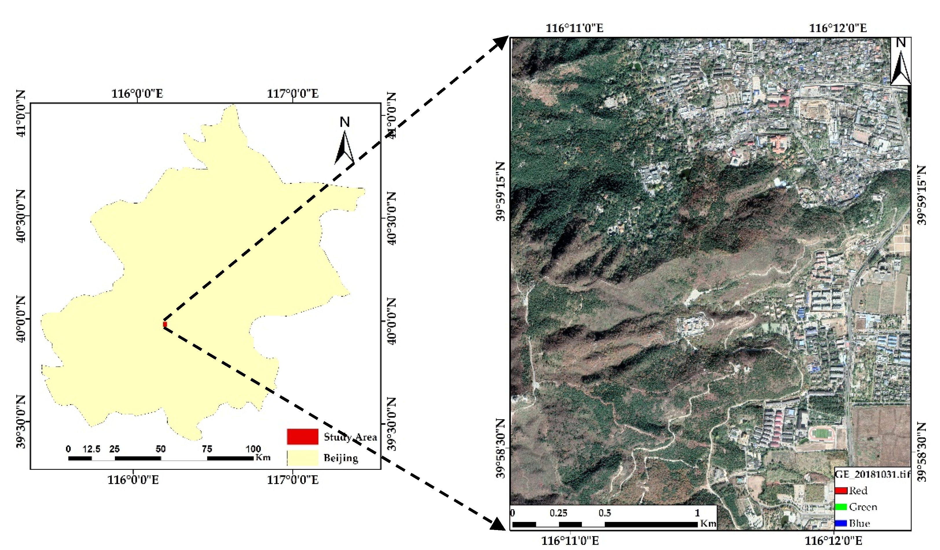
2.1. Study Area

The study area was selected from a typical high-density fixed forest area in the Xishan Forest Park of Beijing, China (39°58′14″ to 39°59′43″N, 116°10′45″ to 116°12′18″E, Figure 1), with a total area of 5.99 km2. The location of Xishan Forest Park features a warm-temperate semi-humid continental monsoon climate with four distinct seasons.
The Xishan Forest Park of Beijing has abundant forest resources. Due to severe human destruction in the past, the natural tree forest only has a few species, such as Ulmus pumila (Ul. p) and Koelreuteria bipinnata (Ko. b). Planted forests occupy a main part of the western suburb of Beijing, such as Pinus tabuliformis (Pi. t), Platycladus orientalis (Pl. o), Robinia pseudoacacia (Ro. p), Acer truncatum (Ac. t), Ginkgo biloba (Gi. b), and Quercus variabilis (Qu. v). According to the phenological features of trees, two phenological periods were classified: the growth period and the senescence period. The growth period is the period from leaf unfolding in the spring to the appearance of leaf discoloration in early autumn and is characterized by leaf unfolding and growth. The senescence period is the period from the first appearance of autumn-colored leaves to the end of defoliation, featuring leaf discoloration and defoliation [41]. As shown in Table 1, seven types of tree species in the study area have different seasonal variation characteristics.

2.2. Materials

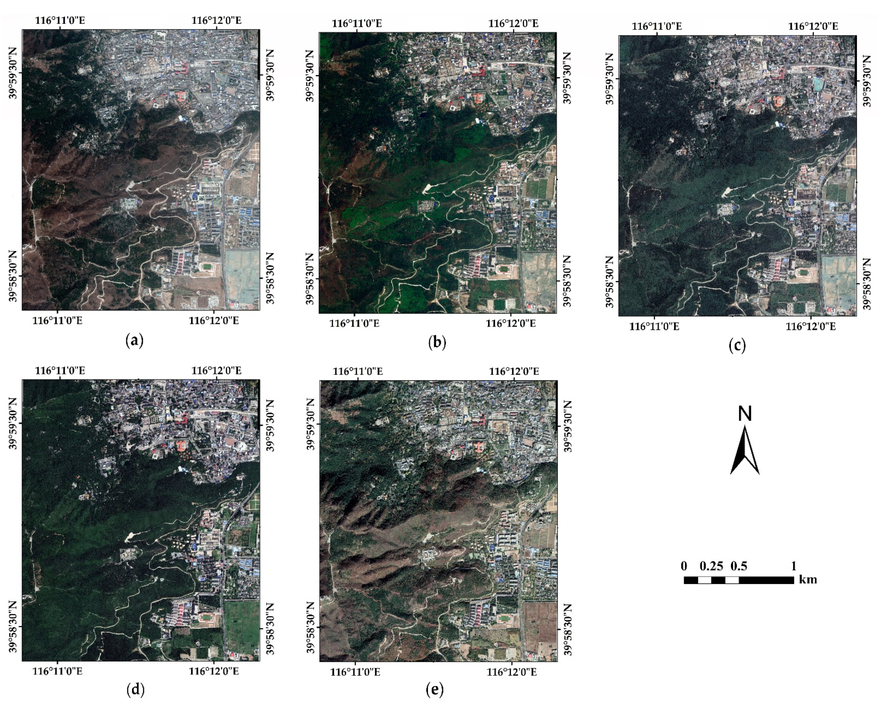
2.2.1. Multitemporal GE Data

Google Earth images are from different multispectral image sources, and the GE images consist of the three primary colors (red, green, and blue). The GE images used in this study were carefully selected to ensure that each image corresponds to a single image source. Moreover, due to the difference in temperature between seasons, broad-leaved forests exhibit significant defoliation in the autumn and regrowth in the spring [42]. Therefore, five high-resolution GE images recorded in different months of 2018 (31 March, 26 April, 11 June, 23 August, and 31 October) [40,43] were employed for ITS classification to explore the seasonal change features of the tree crowns in the growing and senescence periods of broad-leaved forests [41]. All images were in TIF format and had the Universal Transverse Mercator (UTM) projection with datum WGS-1984. As shown in Figure 2, the spatial resolutions of the GE images were all approximately 0.3 m, including the red, green, and blue channels.

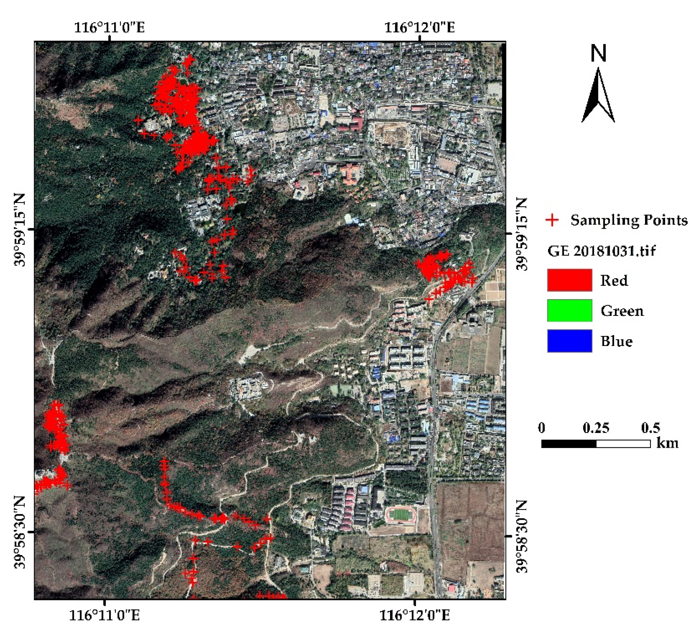
2.2.2. Field Dataset

Two field surveys were carried out in the study area in October and December 2020. Figure 3 shows the sample collection points, and the sample points were all selected near roads, making the coordinates of each sampling point more precise. A Trimble® Geo7X global positioning system (GPS) handheld device (Trimble Inc., Sunnyvale, CA, USA) was utilized to collect the sample points. The species class, DBH, trunk coordinates, and crown radius of each tree were recorded. A camera was employed to take realistic photographs of each sample tree and its surrounding trees to facilitate the identification of the sampled trees on remote sensing imagery. At the end of each day during the field survey, the sampling points were compared with the remote sensing images to confirm the accuracy of the GPS positioning coordinates of each point. A total of 670 trees were collected for seven tree species categories: 120 for Platycladus orientalis, 120 for Pinus tabuliformis, 120 for Robinia pseudoacacia, 70 for Acer truncatum, 100 for Quercus variabilis, 70 for Ginkgo biloba, and 70 for Koelreuteria bipinnata.

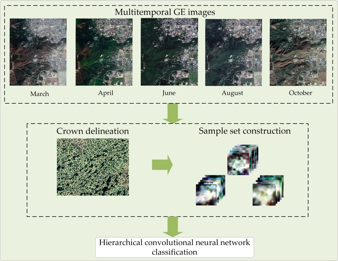
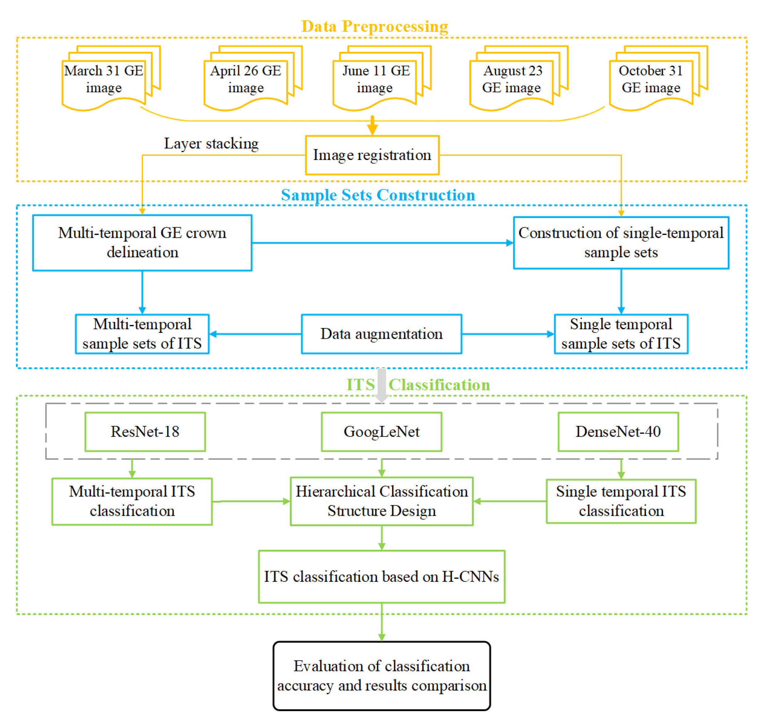
3. Experimental Process

The experimental process consists of four parts: data preprocessing, sample set construction, ITS classification, and the comparison and evaluation of the classification results, as shown in Figure 4.

3.1. GE Preprocessing

In this study, five GE images over the Xishan Forest Park of Beijing were acquired [15,43]. The downloaded GE images did not require radiometric calibration and atmospheric correction. However, there were geometric rectifications for further high-precision tree species classification. Apparent surface objects that did not change on the time-series image were selected as control points in the GE platform, such as road intersections and building corners, and the five obtained GE images were corrected by ENVI 5.3 software so that the roads, buildings, and trees of the five GE images corresponded well to each other. In addition, approximately 20 control points (evenly distributed) were selected for each image, with a root mean square error (RMSE) lower than 0.3 pixels. After geometric rectification, each of the considered sampled points was located in an individual tree crown on the GE images.

3.2. Construction of Remote Sensing Image Sets

To compare the performances of the single- and multitemporal GE data used for ITS classification, two groups of image sets were produced to construct the sample sets in this study. The first group was the single-temporal image set, and five single-temporal image sets were generated from each of the five GE images. The other group was a multitemporal image set, which was formed by stacking the five GE images. After the removal of non-crown areas, tree crown delineation was performed using multitemporal remote sensing images [44]. In addition, this study used the final crown delineation map of the multitemporal GE data for the construction of the subsequent sample sets.

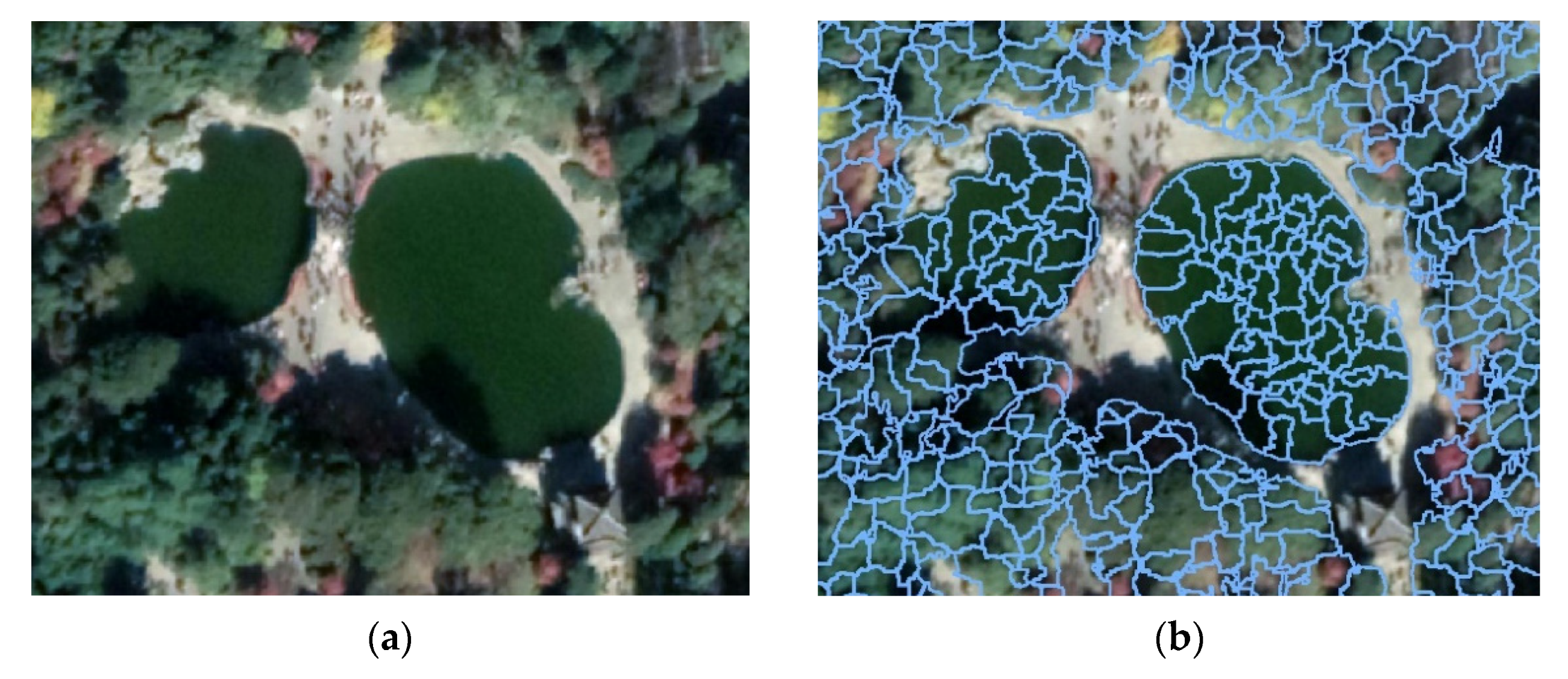
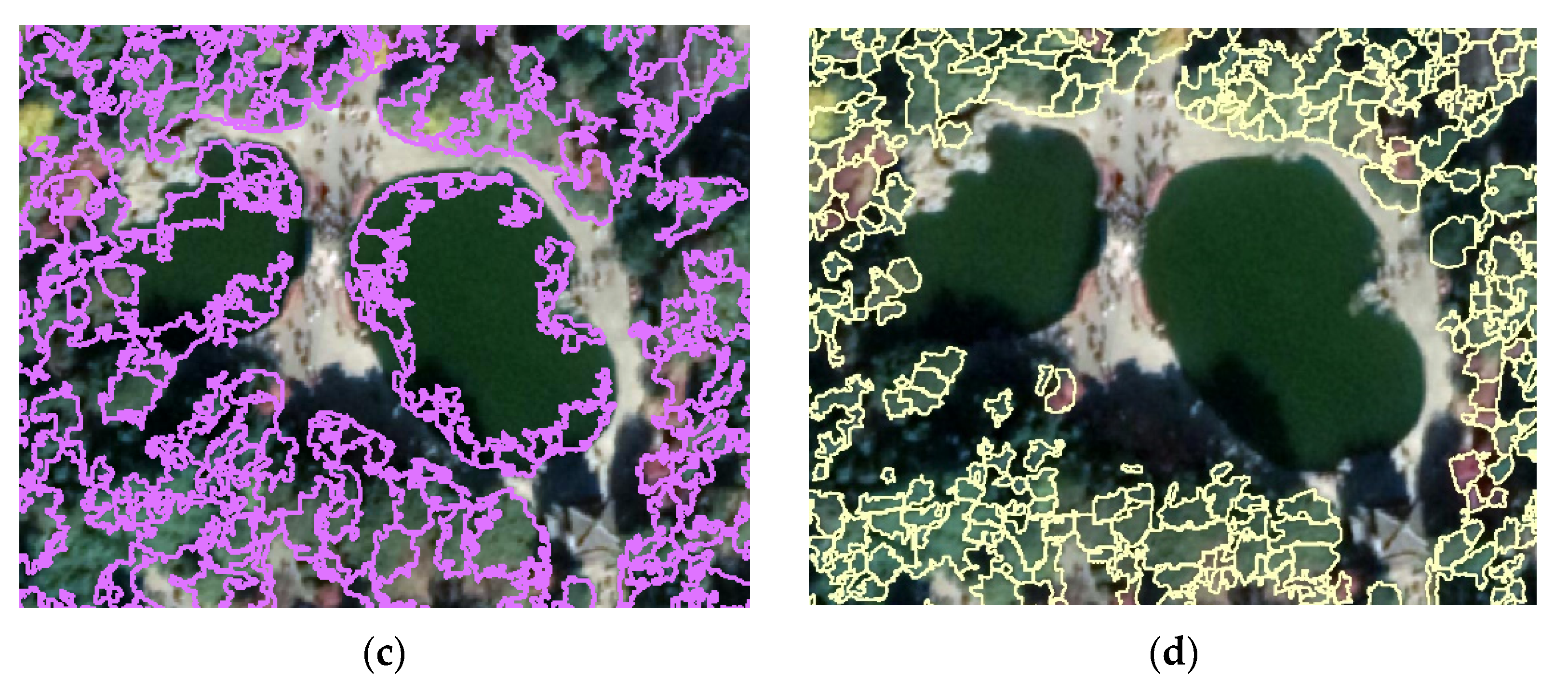
3.2.1. Individual Tree Crown Delineation Using Multitemporal GE Images

The high accuracy of the individual tree crown delineation results facilitates the improvement in ITS classification accuracy [1,25]. The GE images have only red, green, and blue bands and lack near-infrared bands to calculate vegetation indices, such as the normalized difference vegetation index (NDVI). In the study area, the color of several artificial lakes was close to that of vegetation. Furthermore, there was no corresponding water index in the visible band, which leads to difficulties in extracting tree crowns with high precision. Since 1995, Woebbecke et al. have been working on vegetation–soil differentiation based on vegetation indices in the red, green, and blue bands [45]. Subsequently, several indices have been constructed for UAV RGB images to study vegetation coverage, plant heights, and crop growing conditions. These indices include the green–red difference index NGRDI [46], normalized green–blue difference index NGBDI [47], super green–ultra red difference index EXGR [48], green–red vegetation index MGRVI [49], red–green–blue vegetation index RGBVI [50], and other RGB vegetation indices. In this study, several RGB vegetation indices were applied to multitemporal GE images to extract crowns.

RGB Vegetation Indices Used for Multitemporal GE Images

This study utilized the six vegetation indices listed in Table 2 below for crown extraction, where R, G, and B are the results of red, green, and blue channel normalization, respectively. Six groups of vegetation indices were calculated for each of the five GE datasets to obtain 30 different RGB vegetation index images as scalar maps. Thirty scalar maps were compared to select the scalar maps with large differences between vegetation and indistinguishable green non-vegetation features. Then, the combinations with selected scalar maps were combined in different ways, and threshold segmentation was applied. The combination with the optimal threshold segmentation results was selected, which can distinguish tree crowns from non-crown landforms such as water, roads, and buildings. RGBVI was used for the August GE image, MGRVI was used for the October GE image, and the threshold values were set to 0.14 and 0.5, respectively.

Individual Tree Crown Delineation

The method based on multiscale individual crown delineation proposed by Jing et al. [44] was adapted so that it could be applied to multitemporal data. The differences in the scale and spectral features of different crown horizontal slices were also employed, which can effectively reduce oversegmentation and undersegmentation of the crown in dense forests [44]. The specific steps were as follows: (1) Set the target crown horizontal slice size and select a scale sequence with the crown of 2-pixel increments. (2) Transfer the multitemporal GE image to obtain an image that contains a brightness component. (3) Remove the non-vegetation areas in the multitemporal GE image set according to the optimal combination described above. (4) Calculate the similarity of the pixel values of adjacent crowns and merge those with more remarkable similarity into the same crowns (different branches); divide others into various crowns. (5) Integrate all the crown slices generated by step 5. (6) Utilize the integrated layers generated by step 5 as markers and use the watershed approach to segment the image generated by step 2 and yield the individual tree crown delineation map. Figure 5a indicates a GE remote sensing image of crowns with no delineation; Figure 5b displays the result of delineation using one RGB vegetation index for a single-temporal image (any RGB vegetation index was subject to oversegmentation or undersegmentation, as shown in Figure 5b); Figure 5c displays the result of delineation using multiple RGB vegetation indices for a single-temporal image (any RGB vegetation index combination in a single-temporal image was also subject to oversegmentation or undersegmentation); Figure 5d suggests the results of delineation using the optimal vegetation index combination described above for multitemporal images. In Figure 5b,c, there are signs of obvious oversegmentation or undersegmentation, while water bodies, roads, and shadows are better eliminated in Figure 5d. As some crowns were shaded in the other temporal images, they are not delineated in Figure 5d.

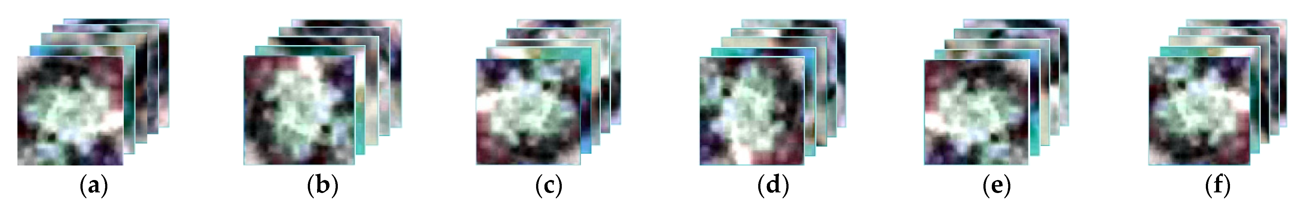
3.2.2. Sample Dataset Construction

The sample datasets were generated with respect to the sample points collected by the field survey. The detailed steps were as follows: (1) The tree polygons in the crown delineation map were labelled according to the tree species and positions of the sampling points. (2) The GE images were clipped according to the smallest outer rectangle of each labelled tree polygon. (3) The clipped subimages were grouped with respect to the labels and then resized to the same image size. Based on the average size of the minimum outer rectangles of the delineated tree crowns, 32 × 32 was chosen as the uniform size for the sample set production [51]. Furthermore, there is a time lag between the collection of sample points and the acquisition of GE images. Therefore, the sample points corresponding to trees that appear highly variable or hidden in shadows were not used to produce a sample image.
A large number of samples is more effective for the training and classification of deep learning methods, so data augmentation was employed to enlarge the sample sets. There are two common methods of data augmentation: geometric transformations and color space transformations. Geometric transformations mainly include flipping, dropout, rotation, cropping, and adding noise. Color space transformations mainly involve saturation, random brightness, and random contrast [52,53]. Moreover, each of five multitemporal remote sensing images was taken at different angles, which caused the trees to tilt and distort in different directions. Therefore, this study utilized the flipping and rotation geometric transformations to augment the number of sample sets. As shown in Figure 6, the original sample set was processed by 90° rotations, 180° rotations, 270° rotations, horizontal flipping, and vertical flipping to augment the sample set to six times the original sample set.
After data augmentation, a total of 3162 sample sets were generated. In addition, the training sets, validation sets, and testing sets were randomly divided in a 3:1:1 ratio before data augmentation, which illustrated the generalization of deep learning classification, with the specific sample numbers shown in Table 3.

3.3. H-CNN Classification

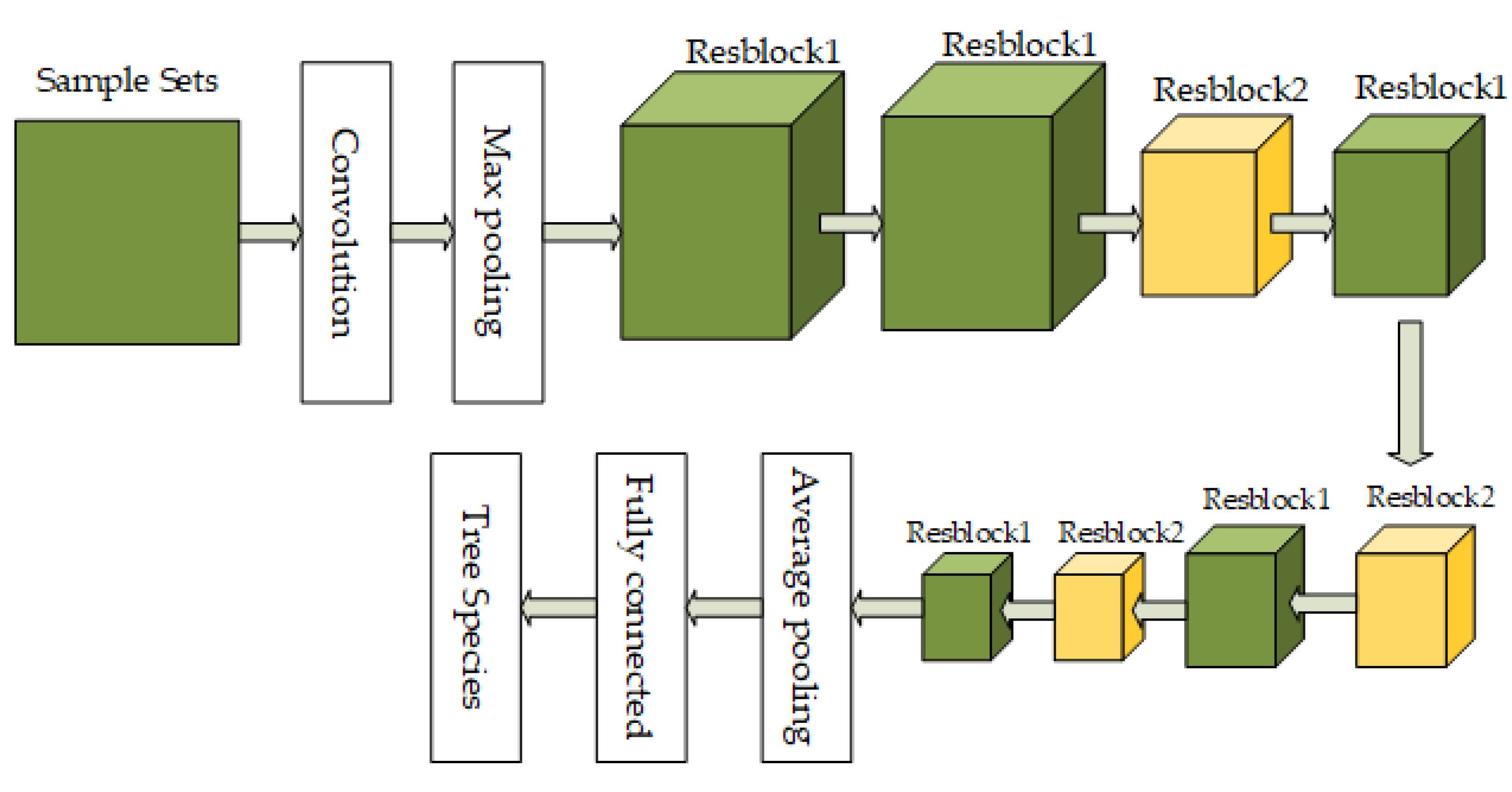
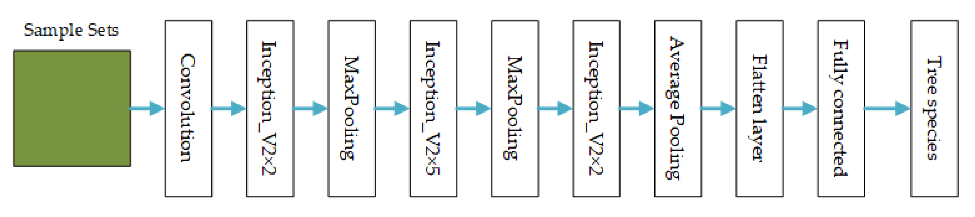
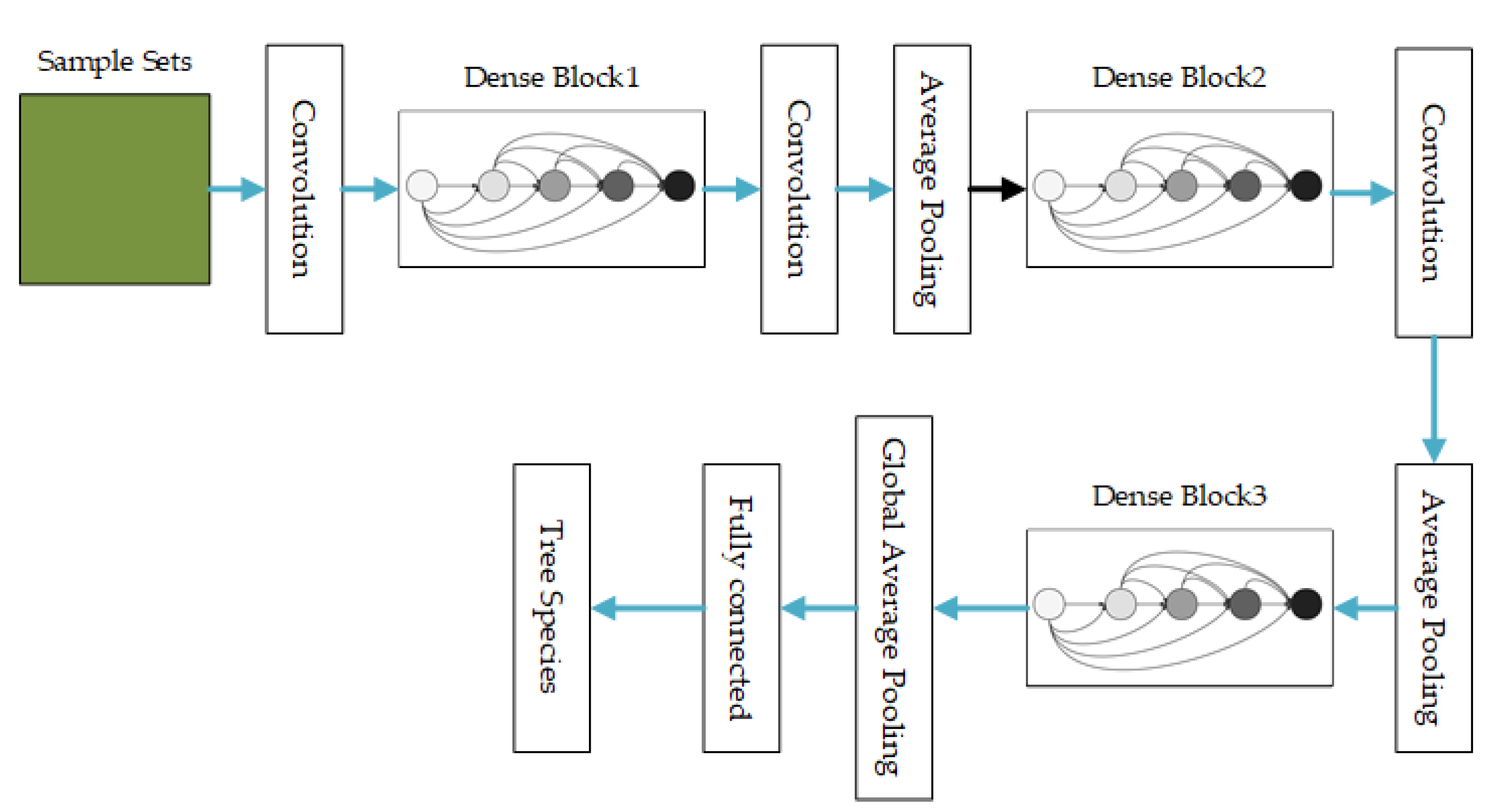
3.3.1. CNN Algorithms

Yan et al. employed ResNet-18 and GoogLeNet for ITS classification, while Li et al. utilized ResNet-18 and DenseNet-40, yielding approximately 7590% classification accuracy for each method [51,54]. Therefore, three CNNs, ResNet-18, GoogLeNet, and DenseNet-40, were selected in this study to combine with the hierarchical classification structure for ITS classification. ResNet, proposed by He et al. [55], won the ILSVRC 2015 competition. The structure of ResNet can accelerate the training of neural networks so that they are extremely fast, and the accuracy of the model has also been improved significantly. Moreover, ResNet-18 has 18 weighting layers, starting with a convolutional layer, then 8 Resblocks (each containing two convolutional layers), and ending with a fully connected layer. The relatively shallow model structure of ResNet-18 is suitable for sample images of a small size (32 × 32) (Figure 7).
GoogLeNet was proposed in 2014 by Szegedy et al. [56]. The Google team clustered sparse matrices into denser submatrices and approximated the optimal sparse structure by constructing dense block structures. Thus, improved performance can be achieved without a large increase in computational effort. The original GoogLeNet model was used to classify the ImageNet image set at 224 × 224 × 3. Thus, it was necessary to modify the network to adapt to the small-scale samples in this study. GoogLeNet consists of one convolutional layer, nine inception modules, two max-pooling layers, one average pooling layer, and one fully connected layer. To make sample sets of the 32 × 32 size function in GoogLeNet, a flattening layer should be added before the fully connected layer, transforming a multidimensional matrix into one dimension. As shown in Figure 8, this modification allows samples of any size with a uniform scale to participate in GoogLeNet.
DenseNet was proposed by Huang et al. [57] in 2017 and won the best paper award at CVPR 2017. DenseNet uses dense blocks with a fully connected layer that alleviates the vanishing gradient problem, enhances feature propagation, and significantly reduces the number of parameters. This structure makes training much more accessible and minimizes overfitting problems for tasks with small training sets (Figure 9).

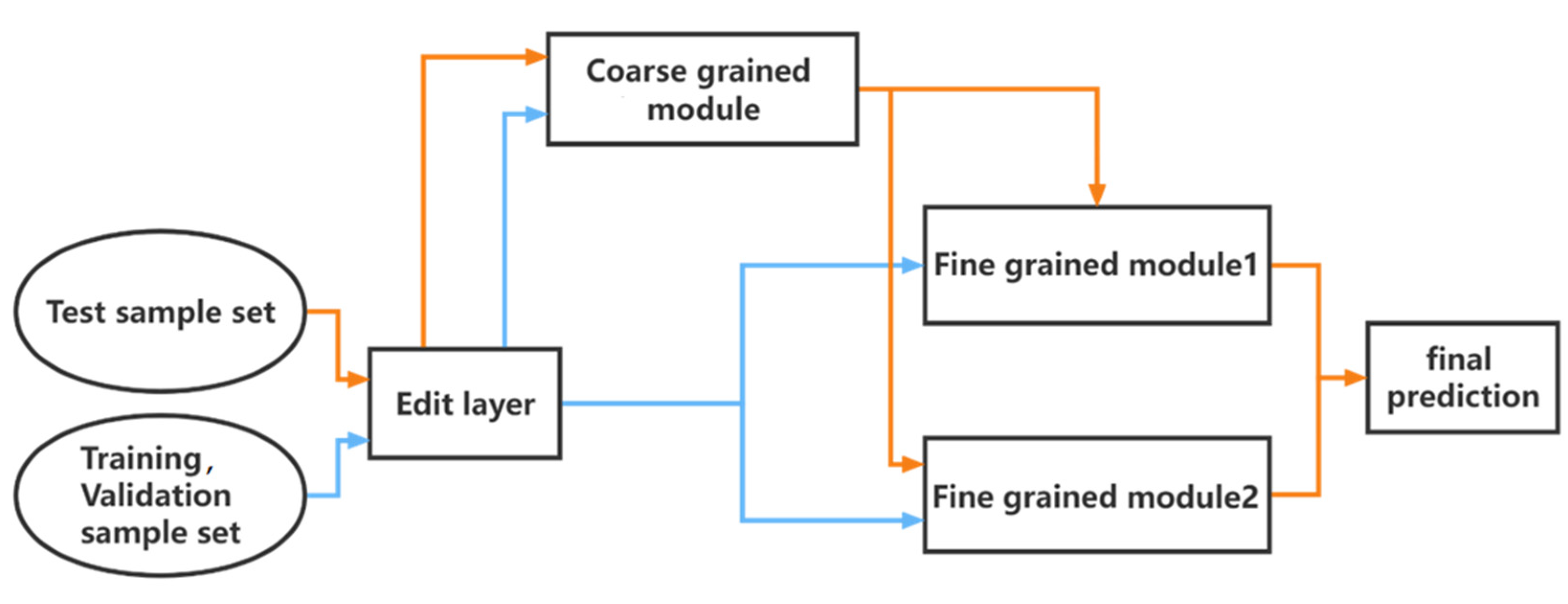
3.3.2. Hierarchical Classification Structure Design

The core of H-CNNs is the construction of tree classifiers. The classification tree structure consists of coarse-grained modules and multiple parallel fine-grained modules. The coarse-grained modules distinguish visually disparate categories, while the fine-grained modules identify the visually less disparate categories. This structure effectively speeds up prediction, reduces computational complexity, and improves the accuracy of predictions within the same level by focusing different levels of classifiers on fewer categories [31,38]. Different from the 3-layer module used by other works [31], this study did not employ a shared layer to merge the first few layers of multiple CNNs. The first few layers of CNNs usually learn information such as the color and edges of sample images [58], while this study requires the classification of tree species based on their color-changing patterns. Therefore, the information acquired by training the first few layers of the CNN is critical and cannot be merged into a CNN shared layer to reduce training time. Although this design increased the number of parameters and the amount of calculation effort, it was essential for the accuracy of the ITS classification.
This study utilized a predefined conceptual tree structure to construct a classifier. Specifically, the considered tree species were divided according to two depths of hierarchy based on different tree species. The flow of the sample set functioning in the H-CNN is shown in Figure 10. The blue line in Figure 10 represents the flow of the input sample set between the modules. The training and validation sample sets were first input into the editing layer, where they were uniformly cropped and further divided into other modules based on category labels. The editing layer connected both coarse-grained and fine-grained modules. Both the coarse- and fine-grained modules consisted of a complete CNN. The yellow line represents the prediction path, where the test sample set passed through the editing layer and entered the coarse- and fine-grained modules sequentially. In the coarse-grained module, the trained coarse-grained classifier performed coarse category predictions on the test sample set. According to the different coarse prediction categories, the test samples were transferred to the corresponding fine-grained module for further fine-grained category prediction. Finally, the classification accuracies of the H-CNN methods were evaluated by comparing the predicted categories with the true labels.

3.3.3. Experimental Environment

The H-CNN classification environment was implemented on a desktop with a Windows 10 OS, an Intel (R) Core (TM) i7-9700K CPU, and an NVIDIA GeForce RTX 2080 Ti GPU. This study employed CUDA11.0 and CUDNN8.0.5 to support the deep learning GPUs [59]. The deep learning framework was built using front-end Keras 2.2.4 and backend TensorFlow 2.4.0, and the programming language was Python 3.7.1.

3.3.4. Training and Prediction

As shown in Table 4, the seven major tree species in the study area were classified into two categories based on their seasonal variation characteristics and tree species attributes. A predetermined conceptual tree structure was constructed based on class I and class II tree species in Table 4. The class I category corresponds to the coarse-grained module, while the class II categories correspond to two different fine-grained modules. To evaluate the effectiveness of the hierarchical classification method combined with the CNNs, three typical CNNs (ResNet-18, GoogLeNet, and DenseNet-40) were trained and utilized to predict ITS separately. According to the misclassification of trees in different CNNs, CNNs with classification advantages for coarse- and fine-grained modules were selected. Then, the advantaged CNNs were set to the corresponding coarse- and fine =-grained modules to form H-CNNs. When the samples were entered into different coarse- and fine- grained modules, the irrelevant category data values were set to 0, which shortened the unnecessary training time and refined the training objectives for each module. Finally, the prediction results of the two types of networks (CNNs and H-CNN) were compared and evaluated. During the training of a CNN, if the accuracy does not improve beyond five iterations, the learning rate was reduced by 0.005. The accuracy improved by 0.001 after five iterations, which was considered an improvement. For the early stop parameter’s setting, the training was ended if the test error increased or the accuracy improvement was less than 0.001 for more than 10 iterations. Based on hierarchical classification, there was a small number and variety of training samples for each module. Therefore, data augmentation was employed in the setting of the training parameters for each module of the H-CNN. Data augmentation included random rotation, random miscut transformation, random zoom in and out, random flipping, and random left–right and top–down shifting. When shifting beyond the original image, ‘reflections’ were used to pad the area. Furthermore, the training parameters of the fine-grained module were fine-tuned according to the performances and the sample image sizes of different CNNs. The learning rate, the number of learning iterations, and the early stop parameters were adjusted to more adequately train the samples. The sample image size, minimum learning rate, and the number of iterations were set to 32 × 32, 0.5 × 10⁻⁶, and 500, respectively.

4. Results

4.1. Classification Accuracy

In this study, three typical CNN models were used to classify each of the six sample sets (five monotemporal GE sample sets and one multitemporal GE sample set), and the confusion matrix was used to assess the accuracy. Furthermore, according to the classification performance of different CNN models, four hierarchical classification CNN models were constructed for multitemporal sample classification. Finally, the accuracy of the H-CNN classification results was evaluated and compared. The evaluation metrics included the overall accuracy (OA, Equation (1)), producer accuracy (PA, Equation (2)), user accuracy (UA, Equation (3)), and kappa coefficient (Equation (4)) [10,60]. Table 5, Table 6, Table 7, Table 8, Table 9 and Table 10 show the classification accuracies of the three typical CNN models for the GE single- and multitemporal testing sets, respectively. According to Table 5, Table 6, Table 7, Table 8, Table 9 and Table 10, Table 5 shows the classification results for the GE image of March. As the leaves had not grown in March, no broad-leaved trees were delineated using the single-temporal image of March 2018. Therefore, only the confusion of conifers and broad-leaved trees in March and the confusion of lateral Platycladus orientalis and Pinus tabuliformis in conifers were discussed. As shown in Table 6, Table 7, Table 8 and Table 9, the highest OA of 77.29% was achieved on the November temporal sample set. On the multitemporal sample set, the ResNet-8 model achieved the lowest OA of 84.37%, and the DenseNet-40 model achieved the highest OA of 89.38%. The accuracy on the multitemporal sample set was significantly higher than the classification accuracy on the single-temporal sample set.
OA = TP + TN TP + TN + FP + FN × 100 %
PA = TP TP + FN
UA = TP TP + FP
Kappa = P o P e 1 P e × 100 %
where TP is true positive, representing the number of correct predictions for positive samples; TN is true negative, showing the number of correct predictions for negative samples; FP is false positive, indicating the number of incorrect predictions for positive samples; FN is false negative, denoting the number of incorrect predictions for negative samples; Po is the number of correctly predicted samples divided by the total number of samples; and Pe is equal to (a1 × b1 + a2 × b2 + … + am × bm)/n × n, where a1 to am represent the number of true samples for each tree species, and b1 to bm indicate the number of samples predicted for each tree species.
In building the hierarchical classification model, the CNNs with the best classification effects at different tree levels need to be selected according to the misclassification of the tree species. In this study, H-CNNs are constructed separately according to the classification of different kinds of sample sets. According to Table 5, Table 6, Table 7, Table 8, Table 9 and Table 10, the number of misclassified samples for different sample sets is shown in Figure 11 (misclassification of the five broadleaf trees in March was not discussed). For the classification of coniferous and broadleaf species using the five single-temporal sample sets, DenseNet-40 had the lowest number of misclassified samples for the March, June, August, and October sample sets. For the classification of Platycladus orientalis and Pinus tabuliformis, DenseNet-40 had the lowest number of misclassified samples for the June, August, and October sample sets. For the classification of five broadleaf species, DenseNet-40 had the lowest number of misclassified samples for the July and August sample sets, whereas GoogLeNet provided the lowest for the March and October sample sets. Therefore, two different H-CNNs, namely, H-CNN1 and H-CNN2, were set up according to the classification of the five single-temporal sample sets. H-CNN1 used DenseNet-40 for the coarse-grained module, the fine-grained module 1, and fine-grained module 2. H-CNN2 employed DenseNet-40 for the coarse-grained module and fine-grained modules 1 and 2. Similarly, with respect to the classification results of the multitemporal sample set shown in Figure 12, another two H-CNNs, namely, H-CNN3 and H-CNN4, were constructed. H-CNN3 used DenseNet-40, ResNet-18, and DenseNet-40 for the coarse-grained module, the fine-grained module 1, and fine-grained module 2, respectively. H-CNN4 employed GoogLeNet, ResNet-18, and DenseNet-40 for the coarse-grained module, fine-grained module 1, and fine-grained module 2, respectively.
The classification results of the four H-CNNs are shown in Table 10. Figure 11 shows a graph of the misclassified sample numbers for different H-CNN models (Figure 12). Comparing Table 5, Table 6, Table 7, Table 8, Table 9, Table 10 and Table 11 and Figure 11 and Figure 12, an OA accuracy of 92.48% was achieved for H-CNN4, which was 15.19% higher than the maximum OA of 77.29% for the single-temporal sample sets, and 3.1% higher than the 89.38% for the multitemporal sample set. Moreover, for the confusion matrices in Table 5, Table 6, Table 7, Table 8, Table 9, Table 10 and Table 11, the bolded words represent the number of correctly classified samples, and the underlined words represent the number of incorrectly classified samples.

4.2. H-CNN vs. CNN Classification Results

The classification results of the four H-CNNs introduced in 4.1 are shown in Table 11 and Figure 12. As shown in Table 10, the results of classifying the multitemporal GE sample set using CNN indicated that the OA results of ResNet-18, GoogLeNet, and DenseNet-40 were 84.37%, 88.35%, and 89.38%, respectively. The four H-CNNs achieved a maximum OA of 92.48% for classifying the multitemporal GE sample set, which was 3.1%–8.11% higher than that of the CNN model. The overall classification accuracy of the H-CNN was significantly improved. The sample confusion of the H-CNN models is shown in Figure 12. Among the classification results of the four H-CNN models, the H-CNN4 model had the lowest number of confusion samples for the coarse-grained module (13 confusion samples). For fine-grained module 1, the H-CNN4 model had the lowest number of confusion samples with 16. For fine-grained module 2, the H-CNN2 model had the lowest numbers of confusion samples (20). The minimum number of confused samples obtained by the coarse- and fine-grained modules corresponding to the CNN for the multitemporal sample set shown in Figure 11 was 23, 19, and 25, respectively. Each module of the CNN had a 5–10 greater number of misclassified samples than the H-CNN, indicating that the H-CNN effectively reduced confusion between tree species.
Furthermore, there are differences between the classification results of different H-CNNs. Compared with H-CNN1 and H-CNN2, the OA value of H-CNN4 yielded increases of 1.62% and 0.89%, respectively. Compared to the other two CNN models, ResNet-18 was employed in H-CNN1 and H-CNN2 to classify Platycladus orientalis and Pinus tabuliformis, which were not adequately trained for the small number of samples. Although the learning rate and early stop parameters were adjusted in this study during hierarchical training, they could not fully compensate for the small number of samples. Therefore, the H-CNNs with ResNet-18 yielded only general classification accuracy for Platycladus orientalis and Pinus tabuliformis. GoogLeNet and DenseNet-40 were slightly better adapted to small sample image sizes, and the H-CNNs with these two models were better at distinguishing Platycladus orientalis and Pinus tabuliformis.

4.3. Comparison of the Classification Results of Different Tree Species

In addition to the resolution of remote sensing data, factors affecting the accuracy of tree species classification include the accuracy of crown extraction and delineation, the number of samples, and the phenological features of the considered tree species, such as the flowering and fruiting periods, flower color, and leaf color. From the single-temporal sample classification results in Table 5, Table 6, Table 7, Table 8 and Table 9, it can be concluded that there was a large number of misclassified samples between Platycladus orientalis and Pinus tabuliformis, Pinus tabuliformis and Robinia pseudoacacia, Robinia pseudoacacia and Koelreuteria bipinnata, and Robinia pseudoacacia and Acer truncatum, and each pair had more than 10 misclassified samples. The multitemporal sample classification results in Table 10 and Table 11 show that Platycladus orientalis, Quercus variabilis, and Ginkgo biloba have better classification accuracy values, where PA > 90% and UA > 80%. Robinia pseudoacacia, Pinus tabuliformis, and Koelreuteria bipinnata have PA values mostly in the range of 70–80%, and misclassification still exists. The reasons for the misclassification can be derived from Table 1. Platycladus orientalis and Pinus tabuliformis are evergreen trees with similar phenological features and leaf shapes. The blooms of Robinia pseudoacacia and Koelreuteria bipinnata are very close, and both have yellowish flowers. Robinia pseudoacacia, Koelreuteria bipinnata, and Acer truncatum have similar leaf colors, varying with season. Robinia pseudoacacia and Pinus tabuliformis show little difference in leaf color during the growing period.

4.4. Comparison of the Classification Results of the Different Sample Sets

In this study, muititemporal GE data consisting of five selected images recorded on 31 March, 26 April, 11 June, 23 August, and 31 October were employed to create a multitemporal sample set. Single-temporal sample sets were also constructed for each of the five GE images. The classification results of the multitemporal sample set were compared with those of the five single-temporal sample sets. As shown in Table 5, the March sample set had the lowest number of misclassifications for conifers and broad-leaved trees and the fewest misclassifications for Platycladus orientalis and Pinus tabuliformis compared to the other single-temporal sample sets. In the April sample set, the classification accuracy of Platycladus orientalis, Pinus tabuliformis, and Quercus variabilis had the highest accuracy, where the PA values were above 70%. Ginkgo biloba and Koelreuteria bipinnata had the lowest accuracy values, and the PA values were below 50%. For the June sample set, only Platycladus orientalis had a PA value that was above 70%, while Koelreuteria bipinnata had a PA value that was below 30%. For the August sample set, Ginkgo biloba had the highest PA value, which was above 85%, while the rest of the species had PA values between 30% and 70%. For the October sample set, Platycladus orientalis, Acer truncatum, Quercus variabilis, and Ginkgo biloba all had PA values that were above 75%, while Koelreuteria bipinnata still had the lowest PA value, which was below 50%. Comparing the results of the four single-temporal sample sets classifications except for March, the October sample set had the highest OA value of up to 77.29%, while the June sample set had the lowest OA value of approximately 60%. The classification accuracies of the October and April sample sets were 1.62% to 14.31% higher than those of the other single-temporal sample sets, respectively, but all of the single-temporal sample set accuracies did not exceed 80%. Table 10 and Figure 11 show the classification results for the multitemporal sample set. The OA values were above 84% and up to 89.38%, which are much higher than the maximum OA values ranging from 7.08% to 12.09% of the single-temporal sample sets. In the multitemporal classification results, all species had PA values above 70%. Koelreuteria bipinnata, which did not exceed 50% in the single-temporal classification, reached a maximum PA value of 92% and a minimum value of 72% in the multitemporal classification task. These findings sufficiently demonstrate that multitemporal data cannot only improve the classification accuracy of indistinguishable tree species but also further reduce the confusion between distinguishable species.

4.5. Classification Map

Based on the classification results in Table 10 and Table 11, the H-CNN4 model corresponding to the multitemporal GE samples with the highest overall classification accuracy was selected for the classification of ITS in the whole study area, and the results are shown in Figure 13. The distribution of Platycladus orientalis and Pinus tabuliformis dominates in the western hills of Beijing, followed by Quercus variabilis, Robinia pseudoacacia, and Acer truncatum, which is in line with the typical mixed forests of northern China.

5. Discussion

5.1. Effect of Combining Multitemporal Data with RGB Vegetation Indices on Crown Delineation

Based on the advantages of RGB vegetation indices applied to UAV RGB imagery to study vegetation and crop growth [47,48,50], this study employed RGB vegetation indices for multitemporal GE remote sensing images to delineate tree crowns. Six vegetation indices (NGRDI, NGBDI, EXG, EXGR, MGRVI, and RGBVI) were used in this study, combined with the color and brightness differences of various features in the multitemporal image. This approach removed the indistinguishable areas of artificial water, shadows, and artificial buildings from the RGB images, which greatly compensated for the lack of near-infrared bands in GE data. Moreover, the shadows in all the single-temporal GE images were excluded from the delineated tree crowns, which provided a solid basis for highly accurate ITS classification. However, several experiments are needed to find the optimal combination of different indices. Furthermore, the images from the multitemporal images of different study areas have different ground objects. Therefore, the optimal combination of RGB vegetation indices should be determined according to the backgrounds of different study areas.

5.2. Influence of the Selection of Multitemporal Data on the Classification of ITS

In this study, five GE images of five different months were selected with respect to the climate of the study area, the tree species, and the trees’ phenological characteristics. It was found that the broad-leaved trees in the study area have not leafed out by March, so they can be well distinguished from the evergreen conifers using the GE image of March. In April, broad-leaved trees leaf out and grow, and they can be easily distinguished from green evergreen conifers according to the differences in greenness between the new and old leaves. At the end of October, the broad-leaved trees are in a period of pigmentation change and defoliation. The Ginkgo biloba leaves turn golden yellow, while the Acer truncatum leaves turn red. These features can be used to better distinguish them from each other using the GE image of October. Moreover, the crowns in June and August are in the flourishing period. In both periods, the crowns and leaves of each tree species have the largest areas, so the GE images covering these two periods were selected to obtain more crown texture information. Therefore, the selection of two temporal images for June and August in this study helped to distinguish between Platycladus orientalis and Pinus tabuliformis, while the amount of data for CNN training was increased. This study used a combination of the above five single-temporal GE images to facilitate the differentiation of the seven major tree species in the study area for multitemporal ITS classification. Compared to the highest OA value of 78.11% achieved by Guo et al. [14], who also used multitemproal high-resolution satellite images of three phases and DenseNet-40, the OA value of DenseNet-40 was 89.38% in this study. The multitemporal GE images consisting of five temporal phases contributed to the significant increase in ITS classification accuracy. The above comparative results illustrate that selecting temporal data according to the categories of the target tree species and their phenological features can increase the differences between tree species and effectively improve the classification accuracy of ITS species.

5.3. Design of the Hierarchical Classification Structure

Hierarchical classification has been gradually applied to tree species classification tasks. For example, Illarionova et al. represented the multiclass forest classification problem as a set of hierarchical binary classification tasks. For each classification task, the researchers selected the most suitable neural network structure to obtain a classification accuracy of up to 77% [12]. Currently, there are few studies that combine hierarchical classification and CNNs for tree species at the individual tree level. Unlike vegetation classification of land cover classes, individual tree species should be considered when constructing a classification tree. Therefore, predefined classification trees based on species attributes are simpler, clearer, and more efficient than those generated by other methods.
In this study, we first classified the sample- and multitemporal images using typical CNNs. Then, a predetermined classification tree structure was built based on the CNN classification results and the species relationship of the considered tree species. Finally, the dominant CNNs were inserted into the corresponding classification modules to improve the accuracy of ITS classification. The H-CNNs obtained the highest accuracy of 92.48%, which increased by 2.66% to 3.72% compared to the highest OA values of typical CNNs. The comparison above illustrates that composing an H-CNN based on advantageous CNNs can improve the accuracy of tree species classification and reduce misclassification. According to the experimental results, there are two factors that affect the classification accuracy of H-CNNs. First, the coarse-grained module in the hierarchical structure was critical. When the coarse-grained module had classification errors, then its submodules (fine-grained modules) could not correctly classify the categories. Second, the hierarchical structure divides the samples into different modules, leading to a reduction in the number of samples. Therefore, a large number of samples is important for the training of the parameters of H-CNNs.

6. Conclusions

This study explored multitemporal high-resolution data consisting of five GE images recorded in different growing periods of tree species for ITS classification. Single- and multitemporal GE sample sets for ITS classification were constructed and classified using three typical CNNs. We explored the potential of low-cost multitemporal GE images for ITS classification in dense forests by comparing the CNN classification results of single- and multitemporal remote sensing images. The hierarchical classification approach combined three typical CNNs to construct four H-CNN models for ITS classification. The classification performance of the four H-CNN models was evaluated by comparing them with the accuracies of CNN-based ITS classification. The results showed that the three CNNs using the multitemporal sample sets offered the highest accuracies, indicating the potential of the low-cost multitemporal GE images used for ITS classification in dense forests. This study combined a predefined hierarchical classification tree structure generated from tree species categories with a corresponding dominant CNN. The construction of the H-CNN had the potential to effectively improve the accuracy of tree species classification and reduce the number of misclassifications. The proposed approach using H-CNN and multitemporal images can help extract ITS information from large-scale dense forests at a relatively low cost and with high accuracy, which could benefit foresters and natural resource managers in their day-to-day operations.
In the H-CNN classification, adjusting the training parameters improved the problem of the small sample size for training each module due to the hierarchical classification structure in the study. However, the small sample problem can be improved in the future by more methods, such as more data augmentation methods based on machine learning or deep learning, and better network model structures for a small number of samples. Furthermore, not every area has a full time series of high-resolution GE remote sensing images. Therefore, in the future, it is possible to make use of other low-cost, large-scale images, such as Gaofen-2, to greatly compensate for the lack of phases in GE multitemporal images for individual tree species classification tasks.

Author Contributions

Conceptualization, Z.L., H.L. and L.J.; Data curation, Z.L.; Funding acquisition, H.L., J.Z., L.J. and Y.T.; Methodology, Z.L. and L.J.; Software, Z.L., H.L. and L.J.; Validation, Z.L. and H.L.; Visualization, Z.L., H.L., J.Z. and H.W.; Writing–original draft, Z.L.; Writing–review & editing, Z.L., H.L. and J.Z. All authors have read and agreed to the published version of the manuscript.

Funding

This research was funded by the Innovative Research Program of the International Research Center of Big Data for Sustainable Development Goals (Grant No.: CBAS2022IRP03); the Aerospace Information Research Institute, Chinese Academy of Sciences (Grant No.: Y951150Z2F); the National Natural Science Foundation of China (Grant No.: 41772347, 41801259, 42071312, 42171291, and 41972308); and the second Tibetan Plateau Scientific Expedition and Research (STEP) (Grant No.: 2019QZKK0806).

Data Availability Statement

Not applicable.

Acknowledgments

The authors would like to thank the Key Laboratory of Digital Earth Science for supporting this research with hardware devices. We thank Changjiang Yuan and Caiyan Chen for their contributions to this research. In addition, we are grateful to the anonymous reviewers who provided helpful comments and suggestions to improve the manuscript.

Conflicts of Interest

The authors declare no conflict of interest.

References

  1. Torabzadeh, H.; Leiterer, R.; Hueni, A.; Schaepman, M.E.; Morsdorf, F. Tree species classification in a temperate mixed forest using a combination of imaging spectroscopy and airborne laser scanning. Agric. For. Meteorol. 2019, 279, 107744. [Google Scholar] [CrossRef]
  2. Komura, R.; Muramoto, K. Classification of forest stand considering shapes and sizes of tree crown calculated from high spatial resolution satellite image. In Proceedings of the 2007 IEEE International Geoscience and Remote Sensing Symposium, Barcelona, Spain, 23–28 July 2007; pp. 4356–4359. [Google Scholar]
  3. Wang, M.; Zheng, Y.; Huang, C.; Meng, R.; Pang, Y.; Jia, W.; Zhou, J.; Huang, Z.; Fang, L.; Zhao, F. Assessing Landsat-8 and Sentinel-2 spectral-temporal features for mapping tree species of northern plantation forests in Heilongjiang Province, China. For. Ecosyst. 2022, 9, 100032. [Google Scholar] [CrossRef]
  4. Kamińska, A.; Lisiewicz, M.; Stereńczak, K. Single tree classification using multi-temporal ALS data and CIR imagery in mixed old-growth forest in Poland. Remote Sens. 2021, 13, 5101. [Google Scholar] [CrossRef]
  5. Fricker, G.A.; Ventura, J.D.; Wolf, J.A.; North, M.P.; Davis, F.W.; Franklin, J. A convolutional neural network classifier identifies tree species in mixed-conifer forest from hyperspectral imagery. Remote Sens. 2019, 11, 2326. [Google Scholar] [CrossRef] [Green Version]
  6. Chemura, A.; van Duren, I.; van Leeuwen, L.M. Determination of the age of oil palm from crown projection area detected from WorldView-2 multispectral remote sensing data: The case of Ejisu-Juaben district, Ghana. ISPRS J. Photogramm. Remote Sens. 2015, 100, 118–127. [Google Scholar] [CrossRef]
  7. Yin, W.; Yang, J.; Yamamoto, H.; Li, C. Object-based larch tree-crown delineation using high-resolution satellite imagery. Int. J. Remote Sens. 2015, 36, 822–844. [Google Scholar] [CrossRef]
  8. Allouis, T.; Durrieu, S.; Vega, C.; Couteron, P. Stem volume and above-ground biomass estimation of individual pine trees from LiDAR data: Contribution of full-waveform signals. IEEE J. Sel. Top. Appl. Earth Obs. Remote Sens. 2013, 6, 924–934. [Google Scholar] [CrossRef]
  9. Jamal, J.; Zaki, N.A.M.; Talib, N.; Saad, N.M.; Mokhtar, E.S.; Omar, H.; Latif, Z.A.; Suratman, M.N. Dominant tree species classification using remote sensing data and object -based image analysis. IOP Conf. Ser. Earth Environ. Sci. 2022, 1019, 012018. [Google Scholar] [CrossRef]
  10. Qin, H.; Zhou, W.; Yao, Y.; Wang, W. Individual tree segmentation and tree species classification in subtropical broadleaf forests using UAV-based LiDAR, hyperspectral, and ultrahigh-resolution RGB data. Remote Sens. Environ. 2022, 280, 113143. [Google Scholar] [CrossRef]
  11. Bergmüller, K.O.; Vanderwel, M.C. Predicting tree mortality using spectral indices derived from multispectral UAV imagery. Remote Sens. 2022, 14, 2195. [Google Scholar] [CrossRef]
  12. Illarionova, S.; Trekin, A.; Ignatiev, V.; Oseledets, I. Neural-based hierarchical approach for detailed dominant forest species classification by multispectral satellite imagery. IEEE J. Sel. Top. Appl. Earth Obs. Remote Sens. 2021, 14, 1810–1820. [Google Scholar] [CrossRef]
  13. Liu, H. Classification of urban tree species using multi-features derived from four-season RedEdge-MX Data. Comput. Electron. Agric. 2022, 194, 106794. [Google Scholar] [CrossRef]
  14. Guo, X.; Li, H.; Jing, L.; Wang, P. Individual tree species classification based on convolutional neural networks and multitemporal high-resolution remote sensing images. Sensors 2022, 22, 3157. [Google Scholar] [CrossRef] [PubMed]
  15. Hill, R.A.; Wilson, A.K.; George, M.; Hinsley, S.A. Mapping tree species in temperate deciduous woodland using time-series multi-spectral data. Appl. Veg. Sci. 2010, 13, 86–99. [Google Scholar] [CrossRef]
  16. Fang, F.; McNeil, B.E.; Warner, T.A.; Maxwell, A.E.; Dahle, G.A.; Eutsler, E.; Li, J. Discriminating tree species at different taxonomic levels using multi-temporal WorldView-3 imagery in Washington D.C., USA. Remote Sens. Environ. 2020, 246, 111811. [Google Scholar] [CrossRef]
  17. Xie, Z.; Chen, Y.; Lu, D.; Li, G.; Chen, E. Classification of land cover, forest, and tree species classes with ZiYuan-3 multispectral and Stereo data. Remote Sens. 2019, 11, 164. [Google Scholar] [CrossRef] [Green Version]
  18. Franklin, S.E.; Ahmed, O.S. Deciduous tree species classification using object-based analysis and machine learning with unmanned aerial vehicle multispectral data. Int. J. Remote Sens. 2018, 39, 5236–5245. [Google Scholar] [CrossRef]
  19. Sun, Y.; Xin, Q.; Huang, J.; Huang, B.; Zhang, H. Characterizing tree species of a tropical Wetland in southern China at the individual tree level based on convolutional neural network. IEEE J. Sel. Top. Appl. Earth Obs. Remote Sens. 2019, 12, 4415–4425. [Google Scholar] [CrossRef]
  20. Zhang, L.; Zhang, L.; Du, B. Deep learning for remote sensing data: A technical tutorial on the state of the art. IEEE Geosci. Remote Sens. Mag. 2016, 4, 22–40. [Google Scholar] [CrossRef]
  21. Krizhevsky, A.; Sutskever, I.; Hinton, G.E. ImageNet classification with deep convolutional neural networks. Commun. ACM 2017, 60, 84–90. [Google Scholar] [CrossRef] [Green Version]
  22. de Souza, I.E.; Falcao, A.X. Learning CNN filters from user-drawn image markers for coconut-tree image classification. IEEE Geosci. Remote Sens. Lett. 2022, 19, 1–5. [Google Scholar] [CrossRef]
  23. Zhang, C.; Sargent, I.; Pan, X.; Li, H.; Gardiner, A.; Hare, J.; Atkinson, P.M. An object-based convolutional neural network (OCNN) for urban land use classification. Remote Sens. Environ. 2018, 216, 57–70. [Google Scholar] [CrossRef] [Green Version]
  24. Zhang, C.; Sargent, I.; Pan, X.; Li, H.; Gardiner, A.; Hare, J.; Atkinson, P.M. Joint deep learning for land cover and land use classification. Remote Sens. Environ. 2019, 221, 173–187. [Google Scholar] [CrossRef] [Green Version]
  25. Zhang, C.; Zhou, J.; Wang, H.; Tan, T.; Cui, M.; Huang, Z.; Wang, P.; Zhang, L. Multi-species individual tree segmentation and identification based on improved mask R-CNN and UAV imagery in mixed forests. Remote Sens. 2022, 14, 874. [Google Scholar] [CrossRef]
  26. Rezaee, M.; Zhang, Y.; Mishra, R.; Tong, F.; Tong, H. Using a VGG-16 network for individual tree species detection with an object-based approach. In Proceedings of the 2018 10th IAPR Workshop on Pattern Recognition in Remote Sensing (PRRS), Beijing, China, 19–20 August 2018; pp. 1–7. [Google Scholar]
  27. Chen, C.; Jing, L.; Li, H.; Tang, Y. A new individual tree species classification method based on the ResU-Net model. Forests 2021, 12, 1202. [Google Scholar] [CrossRef]
  28. Yu, K.; Hao, Z.; Post, C.J.; Mikhailova, E.A.; Lin, L.; Zhao, G.; Tian, S.; Liu, J. Comparison of classical methods and mask R-CNN for automatic tree detection and mapping using UAV imagery. Remote Sens. 2022, 14, 295. [Google Scholar] [CrossRef]
  29. Apostol, B.; Petrila, M.; Lorenţ, A.; Ciceu, A.; Gancz, V.; Badea, O. Species discrimination and individual tree detection for predicting main dendrometric characteristics in mixed temperate forests by use of airborne laser scanning and ultra-high-resolution imagery. Sci. Total Environ. 2020, 698, 134074. [Google Scholar] [CrossRef]
  30. Hologa, R.; Scheffczyk, K.; Dreiser, C.; Gärtner, S. Tree species classification in a temperate mixed mountain forest landscape using random forest and multiple datasets. Remote Sens. 2021, 13, 4657. [Google Scholar] [CrossRef]
  31. Yan, Z.; Zhang, H.; Piramuthu, R.; Jagadeesh, V.; DeCoste, D.; Di, W.; Yu, Y. HD-CNN: Hierarchical deep convolutional neural networks for large scale visual recognition. In Proceedings of the 2015 IEEE International Conference on Computer Vision (ICCV), Santiago, Chile, 13–16 December 2015; pp. 2740–2748. [Google Scholar]
  32. Zheng, Y.; Chen, Q.; Fan, J.; Gao, X. Hierarchical convolutional neural network via hierarchical cluster validity based visual tree learning. Neurocomputing 2020, 409, 408–419. [Google Scholar] [CrossRef]
  33. Waśniewski, A.; Hościło, A.; Chmielewska, M. Can a hierarchical classification of Sentinel-2 data improve land cover mapping? Remote Sens. 2022, 14, 989. [Google Scholar] [CrossRef]
  34. Fan, J.; Zhang, J.; Mei, K.; Peng, J.; Gao, L. Cost-sensitive learning of hierarchical tree classifiers for large-scale image classification and novel category detection. Pattern Recognit. 2015, 48, 1673–1687. [Google Scholar] [CrossRef]
  35. Zhang, H.; Xu, D.; Luo, G.; He, K. Learning multi-level representations for affective image recognition. Neural Comput. Applic. 2022, 34, 14107–14120. [Google Scholar] [CrossRef]
  36. Qiu, Z.; Hu, M.; Zhao, H. Hierarchical classification based on coarse- to fine-grained knowledge transfer. Int. J. Approx. Reason. 2022, 149, 61–69. [Google Scholar] [CrossRef]
  37. Liu, Y.; Suen, C.Y.; Liu, Y.; Ding, L. Scene classification using hierarchical wasserstein CNN. IEEE Trans. Geosci. Remote Sens. 2019, 57, 2494–2509. [Google Scholar] [CrossRef]
  38. Zhao, S.; Jiang, X.; Li, G.; Chen, Y.; Lu, D. Integration of ZiYuan-3 multispectral and stereo imagery for mapping urban vegetation using the hierarchy-based classifier. Int. J. Appl. Earth Obs. Geoinf. 2021, 105, 102594. [Google Scholar] [CrossRef]
  39. Jiang, X.; Zhao, S.; Chen, Y.; Lu, D. Exploring tree species classification in subtropical regions with a modified hierarchy-based classifier using high spatial resolution multisensor Data. J. Remote Sens. 2022, 2022, 1–16. [Google Scholar] [CrossRef]
  40. Fan, J.; Zhou, N.; Peng, J.; Gao, L. Hierarchical Learning of Tree Classifiers for Large-Scale Plant Species Identification. IEEE Trans. Image Process. 2015, 24, 4172–4184. [Google Scholar] [CrossRef]
  41. Xing, X.; Hao, P.; Dong, L. Color characteristics of Beijing’s regional woody vegetation based on natural color system. Color Res. Appl. 2019, 44, 595–612. [Google Scholar] [CrossRef]
  42. Batalova, A.Y.; Putintseva, Y.A.; Sadovsky, M.G.; Krutovsky, K.V. Comparative genomics of seasonal senescence in forest trees. Int. J. Mol. Sci. 2022, 23, 3761. [Google Scholar] [CrossRef]
  43. Li, W.; Dong, R.; Fu, H.; Wang, J.; Yu, L.; Gong, P. Integrating Google Earth imagery with Landsat data to improve 30-m resolution land cover mapping. Remote Sens. Environ. 2020, 237, 111563. [Google Scholar] [CrossRef]
  44. Jing, L.; Hu, B.; Li, J.; Noland, T.; Guo, H. Automated tree crown delineation from imagery based on morphological techniques. IOP Conf. Ser. Earth Environ. Sci. 2014, 17, 012066. [Google Scholar] [CrossRef] [Green Version]
  45. Woebbecke, D.M.; Meyer, G.E.; von Bargen, K.; Mortensen, D.A. Color indices for weed identification under various soil, residue, and lighting conditions. Trans. ASAE 1995, 38, 259–269. [Google Scholar] [CrossRef]
  46. Shimada, S.; Matsumoto, J.; Sekiyama, A.; Aosier, B.; Yokohana, M. A new spectral index to detect Poaceae grass abundance in Mongolian grasslands. Adv. Space Res. 2012, 50, 1266–1273. [Google Scholar] [CrossRef]
  47. Du, M.; Noguchi, N. Monitoring of wheat growth status and mapping of wheat yield’s within-field spatial variations using color images acquired from UAV-camera system. Remote Sens. 2017, 9, 289. [Google Scholar] [CrossRef] [Green Version]
  48. Xie, J.; Zhou, Z.; Zhang, H.; Zhang, L.; Li, M. Combining canopy coverage and plant height from UAV-based RGB images to estimate spraying volume on potato. Sustainability 2022, 14, 6473. [Google Scholar] [CrossRef]
  49. Wan, L.; Li, Y.; Cen, H.; Zhu, J.; Yin, W.; Wu, W.; Zhu, H.; Sun, D.; Zhou, W.; He, Y. Combining UAV-based vegetation indices and image classification to estimate flower number in oilseed rape. Remote Sens. 2018, 10, 1484. [Google Scholar] [CrossRef] [Green Version]
  50. Guo, Z.; Wang, T.; Liu, S.; Kang, W.; Chen, X.; Feng, K.; Zhang, X.; Zhi, Y. Biomass and vegetation coverage survey in the Mu Us sandy land-based on unmanned aerial vehicle RGB images. Int. J. Appl. Earth Obs. Geoinf. 2021, 94, 102239. [Google Scholar] [CrossRef]
  51. Li, H.; Hu, B.; Li, Q.; Jing, L. CNN-Based individual tree species classification using high-resolution satellite imagery and airborne LiDAR data. Forests 2021, 12, 1697. [Google Scholar] [CrossRef]
  52. Chen, L.; Wei, Y.; Yao, Z.; Chen, E.; Zhang, X. Data augmentation in prototypical networks for forest tree species classification using airborne hyperspectral images. IEEE Trans. Geosci. Remote Sens. 2022, 60, 1–16. [Google Scholar] [CrossRef]
  53. Moreno-Barea, F.J.; Jerez, J.M.; Franco, L. Improving classification accuracy using data augmentation on small data sets. Expert Syst. Appl. 2020, 161, 113696. [Google Scholar] [CrossRef]
  54. Yan, S.; Jing, L.; Wang, H. A new individual tree species recognition method based on a convolutional neural network and high-spatial resolution remote sensing imagery. Remote Sens. 2021, 13, 479. [Google Scholar] [CrossRef]
  55. He, K.; Zhang, X.; Ren, S.; Sun, J. Deep residual learning for image recognition. In Proceedings of the 2016 IEEE Conference on Computer Vision and Pattern Recognition (CVPR), Las Vegas, NV, USA, 27–30 June 2016; pp. 770–778. [Google Scholar]
  56. Szegedy, C.; Liu, W.; Jia, Y.; Sermanet, P.; Reed, S.; Anguelov, D.; Erhan, D.; Vanhoucke, V.; Rabinovich, A. Going deeper with convolutions. In Proceedings of the 2015 IEEE Conference on Computer Vision and Pattern Recognition (CVPR), Boston, MA, USA, 7–12 June 2015; pp. 1–9. [Google Scholar]
  57. Huang, G.; Liu, Z.; Van Der Maaten, L.; Weinberger, K.Q. Densely connected convolutional networks. In Proceedings of the 2017 IEEE Conference on Computer Vision and Pattern Recognition (CVPR), Honolulu, HI, USA, 21–26 July 2017; pp. 2261–2269. [Google Scholar]
  58. Zeiler, M.D.; Fergus, R. Visualizing and understanding convolutional networks. In Computer Vision–ECCV 2014; Fleet, D., Pajdla, T., Schiele, B., Tuytelaars, T., Eds.; Lecture Notes in Computer Science; Springer International Publishing: Cham, Germany, 2014; Volume 8689, pp. 818–833. ISBN 978-3-319-10589-5. [Google Scholar]
  59. Minowa, Y.; Kubota, Y.; Nakatsukasa, S. Verification of a deep learning-based tree species identification model using images of broadleaf and coniferous tree leaves. Forests 2022, 13, 943. [Google Scholar] [CrossRef]
  60. Nezami, S.; Khoramshahi, E.; Nevalainen, O.; Pölönen, I.; Honkavaara, E. Tree species classification of drone hyperspectral and RGB imagery with deep learning convolutional neural networks. Remote Sens. 2020, 12, 1070. [Google Scholar] [CrossRef]
Figure 1. Location of the study area.
Remotesensing 14 05124 g001
Figure 2. GE images on (a) 31 March; (b) 26 April; (c) 11 June; (d) 23 August; (e) 31 October 2018.
Remotesensing 14 05124 g002
Figure 3. Field tree species survey.
Remotesensing 14 05124 g003
Figure 4. Experimental flow chart.
Remotesensing 14 05124 g004
Figure 5. Comparison of crown delineation results. (a) A GE remote sensing image of crowns with no delineation; (b) the result of one RGB vegetation index for a single-temporal GE image; (c) the result of multiple RGB vegetation indexes for a single-temporal GE image; (d) the results of the optimal vegetation index combination based on a multitemporal GE image.
Remotesensing 14 05124 g005aRemotesensing 14 05124 g005b
Figure 6. Schematic diagram of data augmentation. (a) Original individual crown sample; (b) 90° rotation; (c) 180° rotation; (d) 270° rotation; (e) horizontal flipping; (f) vertical flipping.
Remotesensing 14 05124 g006
Figure 7. ResNet-18 model structure.
Remotesensing 14 05124 g007
Figure 8. Modified GoogLeNet model structure.
Remotesensing 14 05124 g008
Figure 9. DenseNet-40 model structure.
Remotesensing 14 05124 g009
Figure 10. Flow chart of an H-CNN.
Remotesensing 14 05124 g010
Figure 11. CNN classification number of misclassified samples (a) Number of misclassifications between coniferous and broadleaf trees; (b) Number of misclassifications between Pl. o and Pi. c; (c) Number of misclassifications between five broadleaf species.
Remotesensing 14 05124 g011
Figure 12. Hierarchical classification number of misclassified samples.
Remotesensing 14 05124 g012
Figure 13. Map of the tree species distribution in the western hills of Beijing.
Remotesensing 14 05124 g013
Table 1. Seasonal variation characteristics of tree species.
Tree Species ShorthandFlowering TimeFlower ColorFruiting PeriodFruit ColorLeaf Color ChangeLeaf Shape
Growth PeriodSenescence Period
Pl. oMarch–AprilYellow/CyanOctoberBrownGreenGreenConiferous
Pi. tApril–MayYellowOctoberBrownGreenGreenConiferous
Ro. pJune–JulyLight YellowAugust–OctoberGreenGreenGreen to YellowConiferous
Ac. tApril–MayLight GreenSeptember–OctoberBrownGreenGreen to Yellow to RedConiferous
Qu. vApril–MayGreenSeptemberBrownGreen (from light to dark)Green to Brown to YellowBroadleaf
Gi. bApril–MayGreenSeptember–OctoberWhiteGreen (from light to dark)Green to YellowBroadleaf
Ko. bJune–AugustYellowSeptember–OctoberBrownGreen (from light to dark)Green to Brown to RedBroadleaf
Table 2. RGB vegetation indices.
Abbreviations Vegetation Index NameFormulaReferences
ExGExcess green2G − R − B[45]
NGRDINormalized green–red difference index(G − R)/(G + R)[46]
NGBDINormalized green–blue difference index(G − B)/(G + B)[47]
EXGRExcess green minus excess red2G − R − B − (1.4R − G)[48]
MGRVIModified green–red vegetation index(G2 − R2)/(G2 + R2)[49]
RGBVIRed–green–blue vegetation index(G2 − B × R)/(G2 + B × R)[50]
Table 3. Numbers of sample sets.
Tree SpeciesTraining SamplesValidation SamplesTest SamplesTotal Samples
Pl. o366120120606
Pi. t342114114570
Ro. p372120120612
Ac. t2467878402
Qu. v336108108522
Gi. b1986060318
Ko. b2467878420
Table 4. Classification of tree species categories.
Class I CategoryConifers (Evergreens)Broadleaf (Deciduous) Trees
Class II categoryPl. oPi. tRo. pAc. tQu. vGi. bKo. b
Table 5. ITS classification results for the March sample set.
CNNConfusion MatricesEvaluation Indicators
Tree SpeciesPl. oPi. tRo. pAc. tQu. vGi. bKo. bPAUAOA%/Kappa%
ResNet-18Pl. o1182000000.980.8673.98/
69.38
Pi. t1980070170.700.98
Ro. p0059601180.700.54
Ac. t0018273510.500.47
Qu. v006197310.900.86
Gi. b001612162110.610.85
Ko. b00105121320.530.46
GoogLeNetPl. o10713000000.890.8572.74/
67.71
Pi. t1979450160.690.86
Ro. p0065121330.770.59
Ac. t0061991550.350.61
Qu. v0030103110.950.76
Gi. b0019276860.670.69
Ko. b00144151260.430.55
DenseNet-40Pl. o10911000000.910.8677.73/
73.56
Pi. t1890020040.790.86
Ro. p0072001110.860.73
Ac. t00613112400.240.57
Qu. v0000108001.000.82
Gi. b0011807850.760.72
Ko. b0490126290.480.59
The bolded words represent the number of correctly classified samples, and the underlined words represent the number of incorrectly classified samples.
Table 6. ITS classification results for the April sample set.
CNNConfusion MatricesEvaluation Indicators
Tree SpeciesPl. oPi. tRo. pAc. tQu. vGi. bKo. bPAUAOA%/Kappa
ResNet-18Pl. o9325100010.780.6464.60/
58.21
Pi. t2582100600.720.62
Ro. p11979140250.660.72
Ac. t0415483530.620.51
Qu. v3007853100.790.90
Gi. b42214026120.430.55
Ko. b190121165250.320.45
GoogLeNetPl. o9420060000.780.7970.21/
64.91
Pi. t7960001100.840.66
Ro. p0268260600.680.76
Ac. t0011520960.670.62
Qu. v000890640.830.94
Gi. b2465028150.470.42
Ko. b1609766340.440.58
DenseNet-40Pl. o9024060000.750.7367.70/
61.88
Pi. t1691700000.800.62
Ro. p0258540600.710.70
Ac. t00124453140.560.56
Qu. v6006840120.780.94
Gi. b6601003260.530.59
Ko. b51179013330.420.51
The bolded words represent the number of correctly classified samples, and the underlined words represent the number of incorrectly classified samples.
Table 7. ITS classification results for the June sample set.
CNNConfusion MatricesEvaluation Indicators
Tree SpeciesPl. oPi. tRo. pAc. tQu. vGi. bKo. bPAUAOA%/Kappa%
ResNet-18Pl. o9021101520.750.6955.31/
47.40
Pi. t2976009000.670.63
Ro. p111557177220.460.57
Ac. t0074632200.590.48
Qu. v105111262440.570.59
Gi. b0696224130.400.52
Ko. b021425114220.280.27
GoogLeNetPl. o94121101110.780.7258.70/
51.40
Pi. t2970906000.640.72
Ro. p06542174370.450.48
Ac. t0019510440.650.47
Qu. v6611674410.690.67
Gi. b226613670.600.73
Ko. b012323120190.240.28
DenseNet-40Pl. o9716070000.810.7562.98/
56.35
Pi. t2476205700.670.66
Ro. p213685117140.570.57
Ac. t0012536070.680.51
Qu. v6618272130.670.67
Gi. b0471223140.520.67
Ko. b002412120300.380.52
The bolded words represent the number of correctly classified samples, and the underlined words represent the number of incorrectly classified samples.
Table 8. ITS classification results for the August sample set.
CNNConfusion MatricesEvaluation Indicators
Tree SpeciesPl. oPi. tRo. pAc. tQu. vGi. bKo. bPAUAOA%/Kappa%
ResNet-18Pl. o8455111770.700.6154.28/
46.19
Pi. t32461328490.400.54
Ro. p11866064250.550.58
Ac. t08622236130.280.47
Qu. v10301673060.680.54
Gi. b006005400.900.69
Ko. b115176133230.290.28
GoogLeNetPl. o77210912820.640.6855.31/
47.55
Pi. t2335140148200.310.58
Ro. p11178262200.650.61
Ac. t06102824190.360.48
Qu. v720876690.700.53
Gi. b000505230.870.63
Ko. b64156126290.370.32
DenseNet-40Pl. o8574610710.710.7259.00/
51.88
Pi. t1753101364110.460.58
Ro. p020611303230.510.60
Ac. t01193522010.450.40
Qu. v1000277060.710.59
Gi. b000005640.930.78
Ko. b60175152330.420.42
The bolded words represent the number of correctly classified samples, and the underlined words represent the number of incorrectly classified samples.
Table 9. ITS classification results for the October sample set.
CNNConfusion MatricesEvaluation Indicators
Tree SpeciesPl. oPi. tRo. pAc. tQu. vGi. bKo. bPAUAOA%/Kappa%
ResNet-18Pl. o9912600030.820.6873.45/
68.67
Pi. t2581800000.710.76
Ro. p11490000150.750.75
Ac. t0866216000.790.91
Qu. v6113830140.770.75
Gi. b000005460.900.90
Ko. b49153126290.370.43
GoogLeNetPl. o9225300000.770.6370.80/
65.50
Pi. t2386100000.750.61
Ro. p17227300080.610.75
Ac. t0006612000.850.85
Qu. v602292060.850.79
Gi. b000005190.850.89
Ko. b481810126200.260.47
DenseNet-40Pl. o1200000001.000.7377.29/
73.21
Pi. t2385600000.750.93
Ro. p10687000170.720.84
Ac. t0096216000.790.84
Qu. v600285080.790.73
Gi. b0000048120.800.91
Ko. b60113165370.470.50
The bolded words represent the number of correctly classified samples, and the underlined words represent the number of incorrectly classified samples.
Table 10. ITS classification results for the multitemporal sample set.
CNNConfusion MatricesEvaluation Indicators
Tree SpeciesPl. oPi. tRo. pAc. tQu. vGi. bKo. bPAUAOA%/Kappa%
ResNet-18Pl. o1106004000.930.8884.37/
81.65
Pi. t1389800040.780.89
Ro. p0790050180.720.91
Ac. t001673070.910.84
Qu. v0002103030.940.88
Gi. b000005460.950.85
Ko. b024207630.720.63
GoogLeNetPl. o1095006000.910.8888.35/
86.32
Pi. t15881100000.770.89
Ro. p0684420240.700.88
Ac. t000780001.000.95
Qu. v0000108001.000.93
Gi. b000006001.000.91
Ko. b000006720.920.75
DenseNet-40Pl. o1086006000.900.8689.38/
87.53
Pi. t18841200000.740.88
Ro. p0596600130.800.89
Ac. t000780001.000.93
Qu. v0000108001.000.95
Gi. b000006001.000.91
Ko. b000006720.920.85
The bolded words represent the number of correctly classified samples, and the underlined words represent the number of incorrectly classified samples.
Table 11. ITS classification results for the H-CNNs multitemporal sample set.
ModelEvaluation IndicatorsTree Species
Pl. oPi. tRo. pAc. tQu. vGi. bKo. b
GoogLeNet
ResNet-18
DenseNet-40
H-CNN1Confusion MatrixPl. o985110600
Pi. t139470000
Ro. p0010812000
Ac. t00078000
Qu. v000610200
Gi. b00000582
Ko. b00000078
PA0.820.820.901.000.940.971.00
UA0.880.950.860.810.941.000.97
OA%/Kappa%90.86/89.25
DenseNet-40
ResNet-18
DenseNet-40
H-CNN2Confusion MatrixPl. o1001100603
Pi. t1010310000
Ro. p0610212000
Ac. t00078000
Qu. v000610200
Gi. b00000582
Ko. b00000078
PA0.830.900.851.000.940.971.00
UA0.910.860.990.810.941.000.94
OA%/Kappa%91.59/90.12
DenseNet-40
DenseNet-40
DenseNet-40
H-CNN3Confusion MatrixPl. o113100600
Pi. t1310100000
Ro. p5128406013
Ac. t00078000
Qu. v000010800
Gi. b00000600
Ko. b00200076
PA0.940.890.701.001.001.000.97
UA0.860.890.981.000.901.000.85
OA%/Kappa%91.45/89.94
DenseNet-40
DenseNet-40
GoogLeNet
H-CNN4Confusion MatrixPl. o105600603
Pi. t1010400000
Ro. p049700019
Ac. t00078000
Qu. v000110601
Gi. b00000600
Ko. b00100077
PA0.880.910.811.000.981.000.99
UA0.910.910.990.990.951.000.77
OA%/Kappa%92.48/91.67
The bolded words represent the number of correctly classified samples, and the underlined words represent the number of incorrectly classified samples.
Publisher’s Note: MDPI stays neutral with regard to jurisdictional claims in published maps and institutional affiliations.

