Article

The Response of Land Surface Temperature Changes to the Vegetation Dynamics in the Yangtze River Basin

1
Chongqing Jinfo Mountain Karst Ecosystem National Observation and Research Station, School of Geographical Sciences, Southwest University, Chongqing 400715, China
2
Chongqing Engineering Research Center for Remote Sensing Big Data Application, School of Geographical Sciences, Southwest University, Chongqing 400715, China
3
Key Laboratory of Geospatial Technology for Middle and Lower Yellow River Regions, Henan University, Ministry of Education, Kaifeng 475004, China
*
Author to whom correspondence should be addressed.
Remote Sens. 2022, 14(20), 5093; https://doi.org/10.3390/rs14205093
Submission received: 27 August 2022 / Revised: 14 September 2022 / Accepted: 10 October 2022 / Published: 12 October 2022

Abstract

:
Land surface temperature (LST) is a key parameter in the study of surface energy balance and climate change from local through to global scales. Vegetation has inevitably influenced the LST by changing the surface properties. However, the thermal environment pattern in the Yangtze River Basin (YRB) still remains unclear after the implementation of large-scale ecological restoration projects. In this study, the temporal and spatial variation characteristics of LST were analyzed based on the Theil–Sen estimator, Mann–Kendall trend analysis and Hurst exponent from 2003 to 2021. The relationships between vegetation and LST were further revealed by using correlation analysis and trajectory-based analysis. The results showed that the interannual LST was in a state of fluctuation and rise, and the increasing rate at night time (0.035 °C·yr−1) was faster than that at day time (0.007 °C·yr−1). An obvious cooling trend could be identified from 2007 to 2012, followed by a rapid warming. Seasonally, the warming speed was the fastest in summer and the slowest in autumn. Additionally, it was found that autumn LST had a downward trend of 0.073 °C·yr−1 after 2015. Spatially, the Yangtze River Delta, Hubei province, and central Sichuan province had a significant warming trend in all seasons, except autumn. The northern Guizhou province and Chongqing showed a remarkable cooling trend only in autumn. The Hurst exponent results indicated that the spring LST change was more consistent than the other three seasons. It was found by studying the effect of land cover types on LST changes that sparse vegetation had a more significant effect than dense vegetation. Vegetation greening contributed 0.0187 °C·yr−1 to the increase in LST in winter, which was spatially concentrated in the central region of the YRB. For the other three seasons, vegetation greening slowed the LST increase, and the degree of the effect decreased sequentially in autumn, summer, spring and winter. These results improve the understanding of past and future variations in LST and highlight the importance of vegetation for temperature change mitigation.

Graphical Abstract

1. Introduction

Land surface temperature (LST) is considered a key factor in surface physical processes at the regional and global scales and a crucial parameter for studying the exchange of matter and energy between the surface and atmosphere. Abnormal temperature changes, such as high temperature and heat waves, may pose a serious threat to climate and environmental stability, agricultural production and ecological balance [1,2]. Over the past century, global temperatures have been on an upward trend [3,4,5]. The global average air temperature by 2009 had increased by 0.7–0.8 °C relative to the pre-industrial conditions, and it is estimated to rise by 1.8–4.0 °C over the course of this century [6,7].
Although some studies had investigated the LST variations based on the data of meteorological station observations [8,9,10], studies on LST variability are generally inadequate at the regional and global scale due to the sparse distribution of meteorological stations (especially for the areas with less human intervention), resulting in the lack of temporal and spatial continuity of data [11,12]. Reanalysis data were an effective way to solve this problem. ERA5 reanalysis data, with a spatial resolution of 0.1°, were appropriate for the study of LST and radiation changes in large areas [13]. However, studies have shown that the applicability of reanalysis data was poor in the Tibetan Plateau [14]. The development of remote sensing provides a reliable database for the study of regional and even global LST. Medium resolution imaging spectrometer (MODIS) products have been widely used in the monitoring of LST changes due to their high accuracy (mean error less than 1 k; k is Kelvin, and every change of k is equal to every change of °C) and their ability to provide long-term data [10,15,16]. Studies of LST based on MODIS data have shown that most parts of the globe, especially the southern hemisphere, were experiencing warming [17]; however, the warming rate was discrepant between day time and night time in different regions. For example, there was more variation during the day time than at night time in Iran due to changes in land cover and use [5]. The Tibetan Plateau had a faster warming trend at night time than at day time, with an average rate of 0.069 K·yr−1 and 0.028 K·y−1, respectively, and night-time warming had a large spatial coverage [11]. Through the study of 347 cities in China, it was found that the overall urban heat island intensity at day time (1.25 ± 0.81 °C) was greater than that at night time (0.79 ± 0.43 °C), but the increasing rate of urban heat island at night time was faster than that at day time [18]. In addition, there were significant differences in seasonal LST changes. The most significant warming was found in winter, followed by spring and summer, and the LST in autumn had basically no change in China from 2003 to 2018 [2]. The agricultural ecological belt in northern China showed a warming trend in spring and winter, and a cooling trend occurred in autumn and summer [10]. LST in winter had a strong warming effect at higher elevation in the Andean region [19]. Regional changes in LST can lead to changes in longwave radiation; therefore, the warming and cooling effects can also indirectly affect the global radiation energy balance [20]. Warming in the arctic has been observed to increase the annual downward longwave radiation by 10 to 40 W/m2 [21]. Meanwhile, it was shown that with the increase in surface temperature, a greater proportion of the net radiation was allocated to evaporation, but net radiation decreased due to the increase in the emitted longwave radiation [22]. A further increase in evaporation would lead to the increase in water vapor content in the atmosphere, which changes the characteristics of cloud cover and cloud albedo, thus affecting the atmospheric transmittance, limiting the arrival of shortwave and longwave radiation to the ground, and finally, affecting the radiation balance of the earth–atmosphere coupled system. Therefore, studying the changes in LST can help understand the energy balance. Although previous studies have analyzed past LST changes, they ignored future LST change patterns. The Hurst exponent, as a long-term memory research method, was widely used to study vegetation dynamics but rarely used in the study of LST consistency changes [23]. An experiment that compared the Hurst exponent value of post-random rearrangement LST with the Hurst exponent value of the original time series LST found that both had little difference and were in the same change trend, which showed that the LST trend predicted by the Hurst exponent had scientific rationality and was basically consistent with the actual situation in the future [12]. Therefore, this is a feasible method to explore the future variation patterns by superimposing the change trend of LST and the Hurst exponent value.
As a dynamic parameter, LST variation is controlled by various factors. It was found that precipitation in the southern part of the Qinghai–Tibet Plateau was higher than that in the northern part, resulting in a lower warming rate in the southern part [24]. The LST of most irrigated areas in the world was lower than that of the corresponding non-irrigated areas, indicating that the change of regional soil moisture also affected the change of LST [25]. The large amounts of greenhouse gases and aerosol particles emitted by human activities have significantly increased their concentration in the atmosphere. The change of concentration affected the radiation balance of the climate system by disturbing the radiation process, which caused the change of the global mean LST [26]. In addition, air temperature [1], vegetation [27], land cover [5] and topography [19] were also factors of LST change. Among these, vegetation was proven to be one of the primary factors, which affected the change of LST at the regional and global scale [28,29,30,31,32]. In recent decades, changes in vegetation coverage caused by deforestation and afforestation have had a significant impact on LST. Li et al. [29] found that deforestation caused significant warming in the tropics, up to 0.28 K per decade, and the southern temperate regions showed stronger warming, with a maximum of 0.32 K per decade, while cooling was observed in the northern temperate regions, up to 0.55 K per decade. China’s greening reportedly accounted for a quarter of the global net increase in leaf area, with forests and croplands being the major sources [33]. Therefore, the effects caused by large-scale afforestation and farmland conversion in China on LST in the past 20 years also cannot be ignored. Peng et al. [34] reported that afforestation in China had a cooling effect during the day time and a warming effect at night time. Additionally, the impact of vegetation on LST is related to land cover types. The enormous evapotranspiration of forest, woodland and cropland could cool LST [33], while grassland had a warming effect on LST, mainly depending on the decrease in albedo [31]. The decrease in urban vegetation coverage caused by human activities could accelerate the rise of LST, which was also an important reason for the formation of the urban heat island [35,36]. The relationship between vegetation and LST is affected by different factors. Cloud cover, cloud optical thickness and aerosol content can change atmospheric transmittance and indirectly affect the precipitation process [22,37]. However, due to the control that climatic conditions exert on biophysical characteristics, the evapotranspiration of vegetation was sensitive within a certain precipitation threshold [38], and the evapotranspiration of vegetation would decrease when the precipitation exceeded that threshold. Diurnal temperature range (DTR) can change vegetation phenology. An increase of 1 °C in the DTR of the northern hemisphere can cause the start of the vegetation growing season to be delayed or advanced in different regions [39]. Although previous studies have investigated the relationships between LST and vegetation at day time, night time and different land cover types, the seasonal relationships based on long time series data were not clearly clarified. Additionally, the individual contribution of vegetation change to LST was poorly understood in previous studies.
The YRB, a crucial area of ecological civilization construction, plays an important role in maintaining the ecological balance and security of the adjacent area and even the whole country, China. The large-scale ecological restoration projects’ implementation, such as the shelterbelt system construction project of the YRB, had prompted many studies to focus on the vegetation dynamic [23], albedo variation [28] and evapotranspiration evolution [40]. Due to the complex exchange of energy between the land and atmosphere, the above changes may contribute to variations of LST, which affect the ecological environment and crop growth and development. At the same time, the range of elevation, latitude, slope and aspect of the YRB is relatively large, resulting in an unequal distribution of solar radiation in the region, which may cause the differences of LST [41]. However, the thermal environment pattern in the YRB still remains unclear. In view of this, understanding LST variation and how vegetation affects LST in the YRB will provide a reference for coping with climate change.
Therefore, the objectives of this study were to (1) analyze the temporal and spatial changes of LST in the YRB during the interannual day time and night time, and the four seasons, from 2003 to 2021; (2) study the consistency of LST changes in the YRB based on the Hurst exponent; and (3) explore the relationships between the vegetation dynamic and LST variation.

2. Materials and Methods

2.1. Study Area

The YRB (24°30′N–35°45′N and 90°33′E–122°25′E) is located in southern China (Figure 1a). It is the largest river in China and the third longest river in the world, covering an area of 800,000 square kilometers, accounting for 18.8% of China’s land area. The geographical environment of the YRB is relatively complex, with plateaus, mountains, basins, hills and plains from the western region to the eastern regions (Figure 1b). In terms of climate, the YRB straddles the Qinghai–Tibet Alpine region, the southwest tropical monsoon region and the central China subtropical monsoon region, thus forming a semi-arid region, a semi-humid region and a humid region from the northwest to the southeast.
In this study, the YRB is divided into four sub-basins: the source of the YRB (SYRB), the upper reaches of YRB (UYRB), the middle reaches of YRB (MYRB) and the lower reaches of YRB (LYRB) [42]. The SYRB is located in the east of the Tibetan Plateau, where the temperature is the lowest in the whole basin, with an annual average temperature of −4.4 °C. The Sichuan Basin, Yunnan–Guizhou Plateau and Jinshajiang River Valley in the UYRB form high-temperature closed centers. The annual average temperature in most regions of the MYRB and LYRB is 16–18 °C, which is the highest in the whole basin. The whole basin is rich in forest resources, accounting for more than 25% of the national forest resources (Figure 1c). Because of afforestation and ecological projects, the vegetation coverage in the YRB led to significant changes in the past two decades [27].

2.2. Data Sources

In this study, the LST data between 2003 and 2021 were obtained from the LST product of Aqua MODIS (MYD11A2, 8-day composite, 1 km resolution, Collection 6.1) (http://ladsweb.nascom.nasa.gov (accessed on 9 October 2021). MYD11A2 is obtained by the generalized split-window algorithm [19]. The overpass times of the Aqua satellite (1:30 PM/AM) are close to the times of daily maximum and minimum temperature. Based on version 6.0, version 6.1 products have been improved by undergoing various calibration changes. MRT is used for MODIS data Mosaic and projection transformation, and ArcGIS is used for batch clipping. According to the quality control (QC) documents, grid pixels of average LST error < 1.0 K were extracted to analyze the interannual, day-time, night-time and seasonal LST. Then, the “3σ-Hampel identifier”, a robust method for outlier detection, was used to remove outliers to obtain reliable values [15]. Winter, spring, summer and autumn in this study refer to the periods of December (last year)–February, March–May, June–August and September–November, respectively.
The MODIS normalized difference vegetation index (NDVI) data (MOD13A3, 30-day composite, 1 km spatial resolution, Collection 6.0) (http://ladsweb.nascom.nasa.gov (accessed on 9 October 2021)), representing vegetation coverage, were used to analyze the vegetation dynamics. MOD13A3 is calculated with the distribution function using the atmospheric correction of surface reflectance (bidirectional reflectance distribution function—BRDF) masked by water, clouds, heavy aerosol and cloud shadows [19]. QC documents were used to obtain the NDVI data unaffected by clouds to ensure the accuracy of the results. The pixels with mean NDVI value no greater than zero were excluded from the study to decrease the effects of snow cover and water.
The MODIS land cover type data of 2020 (MCD12Q1, 1-year composite, 1 km resolution, Collection 6.0) (http://ladsweb.nascom.nasa.gov (accessed on 9 October 2021)) were also used in this study. The International Geosphere-Biosphere Program (IGBP) global vegetation classification scheme, with 17 types of vegetation, was combined into 8 classes according to the research of Feng et al. [43] and Yu et al. [4] (Table 1). The shrubland area in the YRB is less than 0.0001%. Therefore, the shrubland was classified as forest in the present study.
In addition, the digital elevation data at a spatial resolution of 500 m and boundary data of the YRB were obtained from the Resource and Environment Science and Data Center (https://www.resdc.cn (accessed on 9 October 2021)).

2.3. Methods

2.3.1. Trend Analysis

(1)
Theil–Sen estimator
The Theil–Sen estimator, a robust nonparametric statistical method for trend analysis, was applied at a pixel scale and river basin scale to analyze the spatial and temporal fluctuations of the LST and NDVI over the period 2003–2021 in this study. Compared with simple linear regression, this method is insensitive to outliers and skewed distributions [11,40]. The trend of LST and NDVI was calculated using the following equation:
S l o p e = m e d i a n x j x i j i , j > i , i = 1 , , n
x j and x i are the value of the time series whose trend is to be analyzed. n is the length of the time series. S l o p e > 0 indicates an increasing trend, and S l o p e < 0 shows a decreasing trend.
Locally weighted scatter point smoothing (LOWESS), based on locally weighted polynomial regression, was used to smooth the time series data of LST [44]. The advantage of LOWESS is that it can make predictions of volatility and cyclical data.
(2)
Mann–Kendall (MK) test
The Theil-Sen estimator cannot judge the significance of a time series trend. Therefore, the MK method is used to test the significance of the trend of the long time series data. It is a nonparametric trend test method, and the advantage of the method is that the samples do not need to follow a normal distribution [4,11,40]. The calculation process is as follows:
(1)
Define the term “ s g n
s g n x j x i = + 1 x j x i > 0     0 x j x i = 0 1 x j x i < 0
(2)
Calculate the MK test statistic S
S = i = 1 n 1 j = i + 1 n s g n x j x i
(3)
Compute the variance
V a r S = n n 1 2 n + 5 18
(4)
The standard normal test statistic Z S is expressed as
Z S = S 1 V a r S S > 0 0 S = 0 S + 1 V a r S S < 0
If Z S > Z 1 α / 2 , this indicates that the data show a significant trend in the detected time series. Z 1 α / 2 is obtained from the standard normal distribution table. In this study, the MK test was run at α = 0.05 significance level. When Z S > 1.65, 1.96 and 2.58, this indicates that the data passed the test with 90%, 95% and 99% confidence interval.

2.3.2. Correlation Analysis

The Pearson correlation coefficient ( R ) was used to calculate the correlation between the average seasonal LST and the average seasonal NDVI. The Pearson correlation coefficient was calculated using the following equation:
R = i = 1 n LST i L S T ¯ NDVI i NDVI ¯ i = 1 n LST i LST ¯ 2 i = 1 n NDVI i NDVI ¯ 2
where i is the monitoring year from 1 to 19. R > 0 means that there is a positive correlation between LST and NDVI. In contrast, R < 0 means that there is a negative correlation between LST and NDVI.

2.3.3. Hurst Exponent

The Hurst exponent ( H ) has been widely used in climatology and vegetation research to evaluate whether the change trend of the time series data is persistent [12,45]. It reflects the autocorrelation of the time series, especially the long-term trend hidden in the series. The Hurst exponent was calculated using the following equations:
(1)
Divide the long time series { LST m } ( m = 1 ,   2 ,   ,   n ) into m subseries X   t , and for each series, t = 1 ,   ,   m
(2)
Define the long-term memory of the time series of the mean LST
L S T ¯ m = 1 m t m L S T m           m = 1 , 2 , , n
(3)
Calculate the accumulated deviation from each mean LST
X t , m = t = 1 t L S T t L S T ¯ m         1 t m
(4)
Define the range sequence of R
R = max 1 t m X t , m lim 1 t m X t , m         m = 1 , 2 , , n
(5)
Define the standard deviation sequence of S
S m = 1 m t = 1 m L S T t L S T m 2 1 / 2         m = 1 , 2 , , n
(6)
Calculate the Hurst exponent
R m S m = c m
(7)
The H value is acquired by fitting the following formula
log R / S n = a + H × log n
The value of H ranges from 0 to 1. The H > 0.5 indicates that the future trend change is consistent with the present research (positive autocorrelation), while the H < 0.5 indicates that the trend change in the future is opposite to the present research (negative autocorrelation).
To reveal the consistency in the dynamic trends of the LST, the results of the trend analysis and the Hurst exponent were superimposed together to obtain coupled information on the consistency and change trends. According to the change trends, p-value and H value, the information can be divided into five grades (Table 2).

2.3.4. Contribution Analysis

Theoretical analysis of potential factors of LST
R n = 1 a l b e d o R s + ε R l σ ε T s 4
R n is the surface net radiation. R s and R l   are the downward shortwave solar radiation and longwave radiation. ε is the surface emissivity; σ is the Stephan–Boltzmann constant ( 5.6697 × 10 8 w / m 2 . K 4 ); and T s is the LST. R l can be further written as the σ T a 4 ( T a is the air temperature) [13,43].
According to the surface energy balance, the earth system is powered mainly by shortwave solar radiation. Part of the shortwave radiation is absorbed by the surface, and the rest is reflected back into the atmosphere, where its distribution is mainly determined by the albedo. The absorbed shortwave radiation heats the ground and reflects upward longwave radiation into the atmosphere, warming the atmosphere. The atmosphere heats up and emits longwave radiation back to the surface. Therefore, the surface temperature depends mainly on the complex distribution of energy sources and the interaction between the surface and the atmosphere. Some studies have shown that surface radiation is correlated with vegetation cover [28,29,30,31,32]. Vegetation can strongly influence atmospheric characteristics and thus atmospheric emissivity through evapotranspiration. Therefore, we analyzed the contribution of vegetation cover to LST change.
To quantify the individual contribution of vegetation change to LST, a trajectory-based method was employed to isolate the comprehensive effects of other factors [43]. The change of LST in the vegetation change regions (significance at p < 0.05) represents the joint influence of vegetation and other factors. The change of LST in the nonchanging vegetation regions (significance at p > 0.05) represents a synthetic result of other factors. The contribution of vegetation to LST was calculated as follows:
C o n v e = L S T V E L S T n o n V e
where C o n v e is the contribution of vegetation change to LST. L S T V E and L S T n o n V e are the change trends of mean LST in regions with vegetation change and without vegetation change, respectively, calculated by the MK test with Sen’s slope. All the statistical analyses were conducted using MATLAB R2017b.

3. Results

3.1. Trend Characteristics of Interannual LST

The interannual average LST exhibited a slight upward trend in the YRB from 2003 to 2021, with change rates of up to 0.020 °C·yr−1 (p < 0.05) (Figure 2a). The upward rate at night time was higher than that of the day time, with the magnitude of 0.035 °C·yr−1 (p < 0.05) and 0.007 °C·yr−1 (p > 0.1), respectively (Figure 2b,c). LOWESS estimated that the change trend of LST in the whole basin was in a state of fluctuation and rise, with two turning points in 2007 and 2012. Because turning points occurred, a piecewise fitting was executed to explore the rate of change for each period. The day time LST showed a significant decreasing (Slope = −0.130 °C·yr−1, p < 0.01) and an unobvious increasing trend (Slope = 0.048 °C·yr−1, p >0.05) from 2003 to 2012 and 2012 to 2021, respectively. The night time LST initially continued to increase until 2007 (Slope = 0.073 °C·yr−1, p > 0.05) but was followed by a decreasing trend until 2012 (Slope = −0.160 °C·yr−1, p > 0.05), after which it rapidly rebounded until 2021 (Slope = 0.017 °C·yr−1, p < 0.05).
The interannual LST warmed and cooled in 74.64 % and 25.36% of the total areas of the YRB, respectively (Figure 3a). The areas’ portion of warming and cooling in day-time LST changed by 20.66% compared with the interannual variation. Among them, the significant warming (p < 0.05) areas decreased by 7.21%, mainly clustered in the central and southwestern UYRB, central MYRB and LYRB. Additionally, the significant cooling (p < 0.05) areas, mainly located in Chongqing and northern Guizhou province (Figure 3b,e), increased by 5.91%. The night-time LST was warming across most regions in the YRB. Only 8.32% of the total area, distributed in the middle of UYRB, experienced a slight cooling (p > 0.05) (Figure 3c,f).

3.2. Seasonal LST Variation

The results on seasonal timescales all revealed a slight upward trend, with a rate of 0.013 °C·yr−1 in winter, 0.029 °C·yr−1 in spring, 0.032 °C·yr−1 (p < 0.1) in summer and 0.010 °C·yr−1 in autumn from 2003 to 2021 (Figure 4a–d). Moreover, we could clearly see that there was an upward trend in winter, spring and summer after 2015, especially in spring, with a more obvious upward trend (Slope = 0.113 °C·yr−1), while there was a slight downward trend in autumn, with a rate of −0.073 °C·yr−1.
In terms of the extent of areas, the warming areas were larger than the cooling areas in the four seasons (Figure 5a–d). In winter and spring, a marked warming occurred in the LYRB, central UYRB and MYRB (p < 0.05), especially in the Yangtze River Delta of LYRB; the warming rate was more than 0.1 °C·yr−1 (p < 0.01), while the SYRB experienced an insignificant cooling trend (p > 0.05) (Figure 5a,b). The warming regions in summer were relatively extensive (75.16%), and a slight warming trend even appeared in the SYRB (Figure 5c). The significant warming areas (p < 0.05) expanded to the west and south of the UYRB compared to winter and spring (Figure 5g). In autumn, a significant warming effect was found in the western and eastern parts of the YRB, accounting for only 4.10% of the total areas of the YRB (p < 0.05). However, 2.22% of the areas observed in northern Guizhou province and Chongqing had experienced obvious cooling, with a decreasing rate of more than 0.1 °C·yr−1 (p < 0.05) (Figure 5h), which was different from the other three seasons.
Over the last 19 years, the change trends in LST varied for different land cover types (Table 3). The value of a significant upward trend ranged from 0.0512 °C·yr−1 (p < 0.05) to 0.1200 °C·yr−1 (p < 0.01), and the regions were mainly distributed in the cropland, grassland and urban land. For the urban land, spring had the largest significant increasing trend value at a rate of 0.1200 °C·yr−1 (p < 0.01), followed by summer and winter with increasing trends of 0.1021 °C·yr−1 (p < 0.01) and 0.0858 °C·yr−1 (p < 0.05), respectively. Similarly, cropland significantly increased (p < 0.05) at large rates in winter and spring (0.0825 °C·yr−1 and 0.0580 °C·yr−1, respectively). As for grassland, only spring had a significant upward trend at a rate of 0.0512 °C·yr−1 (p < 0.05). However, forest and woodland, with high vegetation coverage, and barren land, with sparse vegetation, all showed insignificant change trends in the four seasons.

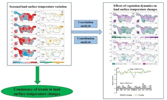
3.3. Consistency of Trends in LST Changes

The areas with Hurst exponent values exceeding 0.5 accounted for 28.54% in winter, 29.21% in spring, 21.47% in summer and 27.79% in autumn. Most areas had Hurst exponent values lower than 0.5, and these regions accounted for more than 70% of the total area of the YRB in four seasons (Figure 6a–d). The information superposition results showed that the region of consistent warming was unevenly distributed in the four sub-basins in autumn and mainly distributed in other areas, except the SYRB, in the other three seasons (Figure 6e–h). The region with consistent cooling was mainly distributed in the SYRB and the junction of UYRB and MYRB in winter, concentrated in the eastern UYRB in autumn and scattered sporadically in the YRB in spring and summer (Figure 6e–h). Generally, the LST in most areas of the YRB was in a state of inconsistent change.

3.4. The Characteristics of the Vegetation Dynamics

The variation of the NDVI trends in the YRB showed the highest and lowest greening rate in winter (0.0044·yr−1) and summer (0.0021·yr−1) from 2003 to 2021 (Figure 7a–d). Spring and autumn increased at a rate of 0.0040·yr−1 and 0.0034·yr−1, respectively (Figure 8a–d). The significant greening regions, accounting for more than 45.85% of the total area in the YRB, mainly occurred in the eastern and middle UYRB and MYRB in the four seasons (Figure 7e–h). The changes in different land cover types showed that the extreme greening trends (p < 0.01) were found in forest, woodland and grassland in the four seasons. Cropland had a greening rate of 0.0031·yr−1 (p < 0.01) and 0.0010 (p < 0.05) in winter and spring, respectively. Wetland showed a significant greening trend (p < 0.05) in spring (0.0011·yr−1) and a significant degradation trend in summer (−0.0016·yr−1). Both urban land and barren land had significant changes (p < 0.05) in summer and autumn (Table 3).

3.5. Contribution of Vegetation Changes to LST

The greening regions (more than 45.85% of the total land areas in the four seasons; Slope > 0, p < 0.05) were much more widespread than the browning regions (less than 2.81%; Slope < 0, p < 0.05) (Figure 7e–h) in the YRB. Therefore, the present study focused mainly on the contribution of greening to the LST variations. In winter, the LST change in the area with vegetation greening was 0.0200 °C·yr−1 and that in the nonchanging area was 0.0013 °C·yr−1. That is, vegetation greening contributed 0.0187 °C·yr−1 to the warming in LST (Figure 8a). In spring and summer, the contribution of vegetation greening was −0.0306 °C·yr−1 and −0.0416 °C·yr−1, respectively (Figure 8b,c). Vegetation greening also had a negative contribution to LST in autumn, with a contribution rate of −0.0672 °C·yr−1, which was slightly stronger than in the spring and summer (Figure 8d).
Considering the spatial distribution of the vegetation, we further analyzed the correlation between LST variations and vegetation dynamics. In the majority of pixels, a positive correlation was observed in winter (65.66%) and spring (56.30%), while a negative correlation was observed in summer (67.99%) and autumn (58.15%) (Figure 9a–d). In winter, the significant positive correlation (11.8%, p < 0.05) was mainly distributed in the north and west of the YRB, and the significant negative correlation (2.60%, p < 0.05) was concentrated in northern Yunnan province (Figure 9e). In spring, the significant correlation (6.90%, p < 0.05) was mainly negative in northern Yunnan province but positive in other areas (5.90%, p < 0.05) (Figure 9f). In summer, 12.61% of the areas showed a strong negative correlation (p < 0.05), most of which were distributed in the UYRB, except for the west (Figure 9g). As for autumn, the significant negative correlation (6.00%, p < 0.05) areas were mainly distributed in the MYRB and LYRB, and the significant positive correlation (3.58%, p < 0.05) areas were mainly scattered in the SYRB and western UYRB (Figure 9h).
The correlation coefficients in different land types varied from −0.691 to 0.632 (Table 3). For grassland and barren land, which were mainly distributed in the plateau, the LST was positively related to vegetation in winter and spring, and these correlations were more significant (p < 0.01) than those in the other seasons. Wetland and cropland showed a significant positive correlation (p < 0.05) in spring, with correlation coefficients of 0.631 and 0.494, respectively, but there was no significant correlation in the other three seasons. Urban LST showed a negative correlation (p < 0.01) with vegetation in summer (−0.691), whereas a positive correlation was found in winter and spring (p < 0.05). Additionally, forest and woodland, which accounted for 59.58% of the total land areas, did not exhibit significant correlations between LST and vegetation.

4. Discussion

4.1. The Spatial and Temporal Change of LST

In the context of global warming, climate change in China, since the 1960s, has been characterized by significant and large-scale warming [9,43,46]. As an important ecological civilization construction region, the YRB also has a certain response to global climate change. Our results suggested that interannual LST has an obvious warming potential, except for Chongqing and northern Yunnan province. This may be related to the positive contribution of CO2 emissions from human activities to global warming. Studies have shown that the 2 °C global warming in the mid-Pliocene was clearly attributable to the increasing CO2 concentration caused by industrialization and urbanization [47,48]. However, asymmetric warming, where the rate was faster at night time than at day time, was found in the YRB (Figure 2). Although the rate of warming at day time was greater than that at night time in some areas, the area of significant warming at night time was twice as large as during the day time (Figure 3b,c). This phenomenon might be driven by changes in cloud cover. Cox et al. [49] argued that increased cloud cover helped keep things cool during the day time but not at night time. Increased cloud cover prevented the loss of ground radiation, which lingered on the surface and acted as a heat preservation effect. From 1984 to 2009, the total cloud cover of MYRB and LYRB showed an increasing trend, and the annual average optical thickness of the Sichuan Basin and the Qinghai–Tibet Plateau increased by more than 0.06·yr−1 [50], which indirectly proved that the asymmetric warming of YRB was related to cloud cover. In addition, high-altitude areas have stronger effects on LST changes at night time than at day time [51,52]. We could clearly see that the LST in the western YRB increased faster at night time than at day time, and the warming area was larger at night time (Figure 3b,c). This result was consistent with the research of Yang et al. [11] in the Tibetan Plateau, who reported that the contributions of elevation to LST variations were 27.12% and 62.98% at day time and night time, respectively.
The National Climate Change Assessment report released by the Chinese government in 2006 predicted that, in the 21st century, the climate in China would continue to warm for the next 20 to 100 years [53]. LST in the YRB all showed a slight upward trend in the four seasons in the past 19 years, which was in agreement with the predicted results. However, the obvious warming occurred in summer (0.032 °C·yr−1), which was contrary to the summer cooling of the agricultural pastural ecotone of northern China [10]. This may be associated with the change of position and intensity of the western Pacific subtropical high (WPSH) system. The sea surface temperature change in the western Pacific triggered a cyclonic circulation on its western side, which was beneficial to the maintenance of WPSH over the YRB, resulting in higher LST in the summer [54]. However, the significant increase in global temperature greatly enhanced the WPSH and moved it westward, which inhibited the water vapor transport in the Indian Ocean [48], thus leading to a significant warming of the Tibetan Plateau. This was the main reason for the apparent warming trend in the western part of the YRB (located on the Tibetan Plateau). Note that the autumn LST showed a slight downward trend after 2015 in the present study, which was mainly attributed to the significant decline of LST in northern Guizhou province and Chongqing (Figure 5d). China’ s National Assessment Report on Climate Change reported that the cooling trend in southwest China recorded in earlier studies was still continuing [53]. Meanwhile, the consistency of trends in LST changes showed that 10% of the YRB area would continue to cool, and 40.96% of the warming regions were likely to experience an opposite trend (Figure 6). These results indicated that the future trend of LST in autumn may decline further.
Although the YRB as a whole showed a warming trend, there was an obvious cooling trend from 2007 to 2012. This phenomenon may be caused by the gap between global changes. Previous studies have shown that the warming trend from 1988 to 2012 was slower than a few decades ago [55,56]. Sun et al. [57] and Du et al. [3] also confirmed that there was a warming gap in China, and the extent of the gap was even more pronounced. The contribution of winter to the national warming gap was the largest, while the contribution of summer was the smallest, which indirectly corresponded to the maximum decreasing rate in winter and the minimum decreasing rate in summer of the YRB from 2007 to 2012.

4.2. Clarification of Biophysical Mechanisms of Interaction between LST and Vegetation

The overall vegetation coverage in the YRB showed a significant improvement trend, and vegetation degradation only occurred in urban land and grassland. This result was consistent with the previous studies in the same area [58,59]. The changes in vegetation coverage would inevitably lead to the variation of evapotranspiration and albedo, thus affecting LST [38].
The alteration of surface thermal properties, particularly decreasing albedo, was shown to be the main reason for controlling the warming effects [43,60]. Specifically, the albedo was reduced by −0.003 ± 0.001, and the surface net shortwave radiation increased by 0.86 ± 0.14 W·m−2 for every 1% increase in NDVI [43]. Vegetation in the eastern part of the Qinghai–Tibet Plateau was significantly greening, while albedo showed a significant decrease for the period 2000 to 2018 [59]. A decrease in albedo resulted in an increase in net radiation from the surface, thus an increase in surface temperature, which explained the positive contribution of vegetation greening to winter LST rise in the central and western regions of the YRB (Figure 8a and Figure 9a). The increasing temperature activated and promoted vegetation photosynthesis and was beneficial to vegetation growth, thus resulting in a positive correlation effect in spring over a large area of the YRB [30,45]. Nevertheless, the positive correlation cannot signify that local LST was rising [33]; for example, grassland and barren land vegetation was greening in winter, but the LST showed a downward trend (Table 3). Similar results were found in the Amur-Heilongjiang River Basin [31]. The positive correlation can be called positive feedback.
By contrast, the cooling effects were more closely related to the increase in evapotranspiration, particularly in summer. Vegetation can change the surface energy flux through evapotranspiration and then change the LST [34,61]. From 1998 to 2017, vegetation restoration in the YRB increased the actual evapotranspiration in most areas, and larger evapotranspiration could decrease the LST and had a negative effect of cooling in the study area [62]. Instead, vegetation degradation increased ground exposure, which prompted more solar radiation being absorbed, and, coupled with less transpiration of vegetation, led to the rise in LST, especially in urban land (Table 3) [35,63]. Meanwhile, high LST usually increased the evaporation of surface water and inhibited the photosynthesis of different vegetation, which would severely limit the growth of vegetation and led to the decline of vegetation greenness [64]. This might be the primary reason for the lowest vegetation greening rate in the YRB in summer, with a value of only 0.0021 °C·yr−1.
Additionally, the effects of evapotranspiration and albedo on LST can be controlled by climatic conditions, to some extent. Evapotranspiration and albedo are relatively sensitive to precipitation within the threshold [38]. The negative correlation found in northern Yunnan province in spring was due to the relatively low precipitation in this region [62], and vegetation cooled the LST by evapotranspiration. Moreover, actual evapotranspiration should increase reasonably with increasing temperature [40]. Studies had shown that rising air temperature could lead to delayed phenology of vegetation and thus promote vegetation greening [33,64]. The bushy vegetation caused an increase in the transpiration and evaporation of water trapped by leaves, and the relatively high temperature also contributed, to some extent, to the increase in actual evapotranspiration, which explained the widespread cooling effect in autumn in the present study.

5. Conclusions

Compared with the commonly used least-square method, Mann–Kendall trend analysis does not require data to meet a certain distribution and is not sensitive to outliers; therefore, it is easier to analyze the change trend of LST in the YRB from 2003 to 2021. The results showed that interannual LST exhibited asymmetric warming, where the increasing rate at night time was faster than that at day time. The change pattern in the four seasons was also different, with the fastest upward rate in summer and the slowest upward rate in autumn. The significant warming areas were mainly distributed in the Yangtze River Delta, Hubei province, and central Sichuan province in all the seasons, except for autumn. Additionally, the northern Guizhou province showed a significant cooling trend in autumn. Moreover, the area of consistent change in LST was the largest in spring and the smallest in summer. Sparse vegetation had a significant positive correlation with LST in winter and spring, and dense vegetation mainly had a negative correlation in summer and autumn. The trajectory-based method showed that vegetation greening played a warming role in LST change in winter, and the opposite effect occurred in the other three seasons. However, LST variations between the area with and without vegetation change may ignore the spatial variability in atmospheric impacts between different regions; therefore, investigating the contribution of vegetation dynamics in the same climatic context in future studies could help mitigate uncertainty.

Author Contributions

Conceptualization, J.L., S.L. and P.Y.; Data curation, J.L.; Formal analysis, J.L.; Funding acquisition, S.L. and P.Y.; Methodology, J.L., X.T., Z.D., M.M. and P.Y.; Project administration, P.Y.; Resources, X.T.; Software, X.T., Z.D. and M.M.; Supervision, S.L. and P.Y.; Writing—original draft, J.L.; Writing—review and editing, J.L., S.L., X.T., Z.D., M.M. and P.Y. All authors have read and agreed to the published version of the manuscript.

Funding

This work was supported by the Fundamental Research Funds for the Central Universities (SWU-KT22009), the National Natural Science Foundation of China (42171175), Strategic Priority Research Program of the Chinese Academy of Sciences (XDA28110201), and the Open Fund of Key Laboratory of Geospatial Technology for the Middle and Lower Yellow River Regions (Henan University), Ministry of Education (GTYR202202).

Data Availability Statement

The data used in this study were obtained from the following platforms: the LAADS of NASA for the MODIS products (http://ladsweb.nascom.nasa.gov (accessed on 9 October 2021)), the Resource and Environment Science and Data Center for the digital elevation data and boundary data (https://www.resdc.cn (accessed on 9 October 2021)).

Acknowledgments

We would like to thank the LAADS of NASA for providing the MODIS products (http://ladsweb.nascom.nasa.gov (accessed on 15 October 2021)) and the Resource and Environment Science and Data Center for providing the digital elevation data and boundary data (https://www.resdc.cn (accessed on 15 October 2021)).

Conflicts of Interest

The authors declare no conflict of interest.

References

  1. Yan, Y.; Mao, K.; Shi, J.; Piao, S.; Shen, X.; Dozier, J.; Liu, Y.; Ren, H.-L.; Bao, Q. Driving forces of land surface temperature anomalous changes in North America in 2002–2018. Sci. Rep. 2020, 10, 1–13. [Google Scholar] [CrossRef] [Green Version]
  2. Zhao, B.; Mao, K.B.; Cai, Y.L.; Meng, J.X. Study of the temporal and spatial evolution law of land surface temperature in China. Remote Sens. Land Resour. 2020, 32, 233–240. [Google Scholar]
  3. Du, Q.; Zhang, M.; Wang, S.; Che, C.; Ma, R.; Ma, Z. Changes in air temperature over China in response to the recent global warming hiatus. J. Geogr. Sci. 2019, 29, 496–516. [Google Scholar] [CrossRef] [Green Version]
  4. Yu, Y.; Duan, S.-B.; Li, Z.-L.; Chang, S.; Xing, Z.; Leng, P.; Gao, M. Interannual Spatiotemporal Variations of Land Surface Temperature in China From 2003 to 2018. IEEE J. Sel. Top. Appl. Earth Obs. Remote Sens. 2021, 14, 1783–1795. [Google Scholar] [CrossRef]
  5. Moradi, M.; Darand, M. Trend analysis of land surface temperature over Iran based on land cover and topography. Int. J. Environ. Sci. Technol. 2022, 19, 1–14. [Google Scholar] [CrossRef]
  6. Easterling, D.R.; Wehner, M.F. Is the climate warming or cooling? Geophys. Res. Lett. 2009, 36, L08706. [Google Scholar] [CrossRef] [Green Version]
  7. European Environmental Agency. The European Environment State and Outlook 2010-Assessment of Global Megatrends; European Environmental Agency: Copenhagen, Denmark, 2010. [Google Scholar]
  8. Feng, J.M.; Liu, Y.H.; Yan, Z.W. Analysis of surface air temperature warming rate of China in the last 50 years (1962–2011) using k-means clustering. Theor. Appl. Climatol. 2015, 120, 785–796. [Google Scholar]
  9. Cao, L.; Zhu, Y.; Tang, G.; Yuan, F.; Yan, Z. Climatic warming in China according to a homogenized data set from 2419 stations. Int. J. Climatol. 2016, 36, 4384–4392. [Google Scholar] [CrossRef] [Green Version]
  10. Wei, B.; Bao, Y.; Yu, S.; Yin, S.; Zhang, Y. Analysis of land surface temperature variation based on MODIS data a case study of the agricultural pastural ecotone of northern China. Int. J. Appl. Earth Obs. Geoinf. ITC J. 2021, 100, 102342. [Google Scholar] [CrossRef]
  11. Yang, M.; Zhao, W.; Zhan, Q.; Xiong, D. Spatiotemporal Patterns of Land Surface Temperature Change in the Tibetan Plateau Based on MODIS/Terra Daily Product From 2000 to 2018. IEEE J. Sel. Top. Appl. Earth Obs. Remote Sens. 2021, 14, 6501–6514. [Google Scholar] [CrossRef]
  12. Yu, Z. Changes of Ground Temperature in Sichuan and Evaluation Model; Cheng University of Technology: Chengdu, China, 2017. [Google Scholar]
  13. Mazhar, U.; Jin, S.; Duan, W.; Bilal, M.; Ali, A.; Farooq, H. Spatio-Temporal Trends of Surface Energy Budget in Tibet from Satellite Remote Sensing Observations and Reanalysis Data. Remote Sens. 2021, 13, 256. [Google Scholar] [CrossRef]
  14. He, Y.F.; Chen, C.; Li, B.; Zhang, Z.L. Prediction of near-surface air temperature in glacier regions using ERA5 data and the random forest regression method. Remote Sens. Appl. Soc. Environ. 2022, 28, 2352–9385. [Google Scholar]
  15. Duan, S.-B.; Li, Z.-L.; Li, H.; Göttsche, F.-M.; Wu, H.; Zhao, W.; Leng, P.; Zhang, X.; Coll, C. Validation of Collection 6 MODIS land surface temperature product using in situ measurements. Remote Sens. Environ. 2019, 225, 16–29. [Google Scholar] [CrossRef]
  16. Zhang, Z.; Lin, A.; Zhao, L.; Zhao, B. Attribution of local land surface temperature variations response to irrigation over the North China Plain. Sci. Total Environ. 2022, 826, 154104. [Google Scholar] [CrossRef] [PubMed]
  17. Mao, K.; Ma, Y.; Tan, X.; Shen, X.; Liu, G.; Li, Z.; Chen, J.; Xia, L. Global surface temperature change analysis based on MODIS data in recent twelve years. Adv. Space Res. 2016, 59, 503–512. [Google Scholar] [CrossRef] [Green Version]
  18. Liu, Y.X.; Yang, Y.B.; Hu, J.; Meng, X.J.; Kuang, K.X.; Hu, X.J.D.; Bao, Y. Temporal and spatial characteristics of diurnal surface urban heat island intensity in China based on long time series MODIS data. Int. J. Geogr. Inf. Sci. 2022, 24, 981–995. [Google Scholar]
  19. Aguilar-Lome, J.; Espinoza-Villar, R.; Espinoza, J.-C.; Rojas-Acuña, J.; Willems, B.L.; Leyva-Molina, W.-M. Elevation-dependent warming of land surface temperatures in the Andes assessed using MODIS LST time series (2000–2017). Int. J. Appl. Earth Obs. Geoinf. ITC J. 2019, 77, 119–128. [Google Scholar] [CrossRef]
  20. Vargas Zeppetello, L.R.; Donohoe, A.; Battisti, D.S. Does surface temperature respond to or determine downwelling longwave radiation? Geophys. Res. Lett. 2019, 46, 2781–2789. [Google Scholar] [CrossRef] [Green Version]
  21. Kim, H.-M.; Kim, B.-M. Relative Contributions of Atmospheric Energy Transport and Sea Ice Loss to the Recent Warm Arctic Winter. J. Clim. 2017, 30, 7441–7450. [Google Scholar] [CrossRef]
  22. Boucher, O.; Randall, D.; Artaxo, P.; Bretherton, C.; Feingold, G.; Forster, P.; Kerminen, V.M.; Kondo, Y.; Liao, H.; Lohmann, U.; et al. Clouds and Aerosols. In Climate Change 2013: The Physical Science Basis; Cambridge University Press: Cambridge, UK, 2014; pp. 571–657. [Google Scholar]
  23. Chen, W.; Bai, S.; Zhao, H.; Han, X.; Li, L. Spatiotemporal analysis and potential impact factors of vegetation variation in the karst region of Southwest China. Environ. Sci. Pollut. Res. 2021, 28, 61258–61273. [Google Scholar] [CrossRef]
  24. Duan, J.; Li, L.; Fang, Y. Seasonal spatial heterogeneity of warming rates on the Tibetan Plateau over the past 30 years. Sci. Rep. 2015, 5, srep11725. [Google Scholar] [CrossRef] [PubMed] [Green Version]
  25. Yang, Q.; Huang, X.; Tang, Q. Global assessment of the impact of irrigation on land surface temperature. Sci. Bull. 2020, 65, 1440–1443. [Google Scholar] [CrossRef]
  26. Zhang, H.; Wang, F.; Wang, F.; Li, J.D.; Chen, X.L.; Wang, Z.Z.; Li, J.; Zhou, X.X.; Wang, Q.Y.; Wang, H.B.; et al. Research progress of cloud radiation feedback in global climate change. Sci. China Earth Sci. 2022, 52, 400–417. [Google Scholar]
  27. Yu, P.; Li, Y.; Liu, S.; Liu, J.; Ding, Z.; Ma, M.; Tang, X. Afforestation influences soil organic carbon and its fractions associated with aggregates in a karst region of Southwest China. Sci. Total Environ. 2022, 814, 152710. [Google Scholar] [CrossRef]
  28. Zhang, Y.-X.; Wang, Y.-K.; Fu, B.; Dixit, A.M.; Chaudhary, S.; Wang, S. Impact of climatic factors on vegetation dynamics in the upper Yangtze River basin in China. J. Mt. Sci. 2020, 17, 1235–1250. [Google Scholar] [CrossRef]
  29. Li, Y.; Zhao, M.; Mildrexler, D.J.; Motesharrei, S.; Mu, Q.; Kalnay, E.; Zhao, F.; Li, S.; Wang, K. Potential and Actual impacts of deforestation and afforestation on land surface temperature. J. Geophys. Res. Atmos. 2016, 121, 14372–14386. [Google Scholar] [CrossRef]
  30. Jiang, L.L.; Guli, J.; Bao, A.M.; Guo, H.; Ndayisaba, F. Vegetation dynamics and responses to climate change and human activities in Central Asia. Sci. Total Environ. 2017, 599–600, 967–980. [Google Scholar] [CrossRef] [PubMed]
  31. Chu, H.; Venevsky, S.; Wu, C.; Wang, M. NDVI-based vegetation dynamics and its response to climate changes at Amur-Heilongjiang River Basin from 1982 to 2015. Sci. Total Environ. 2018, 650, 2051–2062. [Google Scholar] [CrossRef]
  32. Yuan, G.; Tang, W.; Zuo, T.; Li, E.; Zhang, L.; Liu, Y. Impacts of afforestation on land surface temperature in different regions of China. Agric. For. Meteorol. 2022, 318. [Google Scholar] [CrossRef]
  33. Xue, Y.; Lu, H.; Guan, Y.; Tian, P.; Yao, T. Impact of thermal condition on vegetation feedback under greening trend of China. Sci. Total Environ. 2021, 785, 147380. [Google Scholar] [CrossRef]
  34. Peng, S.-S.; Piao, S.; Zeng, Z.; Ciais, P.; Zhou, L.; Li, L.Z.X.; Myneni, R.B.; Yin, Y.; Zeng, H. Afforestation in China cools local land surface temperature. Proc. Natl. Acad. Sci. USA 2014, 111, 2915–2919. [Google Scholar] [CrossRef] [PubMed] [Green Version]
  35. Peng, J.; Ma, J.; Liu, Q.; Liu, Y.; Hu, Y.; Li, Y.; Yue, Y. Spatial-temporal change of land surface temperature across 285 cities in China: An urban-rural contrast perspective. Sci. Total Environ. 2018, 635, 487–497. [Google Scholar] [CrossRef] [PubMed]
  36. Xiao, R.; Cao, W.; Liu, Y.; Lu, B. The impacts of landscape patterns spatio-temporal changes on land surface temperature from a multi-scale perspective: A case study of the Yangtze River Delta. Sci. Total Environ. 2022, 821, 153381. [Google Scholar] [CrossRef] [PubMed]
  37. Srivastava, A.; Rodriguez, J.; Saco, P.; Kumari, N.; Yetemen, O. Global Analysis of Atmospheric Transmissivity Using Cloud Cover, Aridity and Flux Network Datasets. Remote Sens. 2021, 13, 1716. [Google Scholar] [CrossRef]
  38. Zhou, D.; Xiao, J.; Frolking, S.; Liu, S.; Zhang, L.; Cui, Y.; Zhou, G. Croplands intensify regional and global warming according to satellite observations. Remote Sens. Environ. 2021, 264, 112585. [Google Scholar] [CrossRef]
  39. Huang, Y.; Jiang, N.; Shen, M.; Guo, L. Effect of preseason diurnal temperature range on the start of vegetation growing season in the Northern Hemisphere. Ecol. Indic. 2020, 112, 106161. [Google Scholar] [CrossRef]
  40. Zhan, M.Y.; Wang, G.J.; Lu, J.; Chen, L.Q.; Zhu, C.X.; Jiang, T.; Wand, Y.J. Projected evapotranspiration and the influencing factors in the Yangtze River Basin based on CMIP6 models. Trans. Atmos. Sci. 2020, 43, 1115–1126. [Google Scholar]
  41. Wang, L.; Qiu, X.; Wang, P.; Wang, X.; Liu, A. Influence of complex topography on global solar radiation in the Yangtze River Basin. J. Geogr. Sci. 2014, 24, 980–992. [Google Scholar] [CrossRef] [Green Version]
  42. Deng, Y.; Jiang, W.; Tang, Z.; Ling, Z.; Wu, Z. Long-Term Changes of Open-Surface Water Bodies in the Yangtze River Basin Based on the Google Earth Engine Cloud Platform. Remote Sens. 2019, 11, 2213. [Google Scholar] [CrossRef] [Green Version]
  43. Feng, H.; Zou, B. A greening world enhances the surface-air temperature difference. Sci. Total Environ. 2018, 658, 385–394. [Google Scholar] [CrossRef]
  44. Song, Z.; Yang, H.; Huang, X.; Yu, W.; Huang, J.; Ma, M. The spatiotemporal pattern and influencing factors of land surface temperature change in China from 2003 to 2019. Int. J. Appl. Earth Obs. Geoinf. ITC J. 2021, 104, 102537. [Google Scholar] [CrossRef]
  45. Jiapaer, G.; Liang, S.L.; Yi, Q.X.; Liu, J.P. Vegetation dynamics and responses to recent climate change in Xinjiang using leaf area index as an indicator. Ecol. Indic. 2015, 58, 64–76. [Google Scholar]
  46. Wang, X.; Xiao, J.; Li, X.; Cheng, G.; Ma, M.; Zhu, G.; Arain, M.A.; Black, T.A.; Jassal, R.S. No trends in spring and autumn phenology during the global warming hiatus. Nat. Commun. 2019, 10, 1–10. [Google Scholar] [CrossRef] [PubMed] [Green Version]
  47. Zhao, J.; Zhang, S.; Yang, K.; Zhu, Y.; Ma, Y. Spatio-Temporal Variations of CO2 Emission from Energy Consumption in the Yangtze River Delta Region of China and Its Relationship with Nighttime Land Surface Temperature. Sustainability 2020, 12, 8388. [Google Scholar] [CrossRef]
  48. Huang, X.; Yang, S.; Haywood, A.; Jiang, D.; Wang, Y.; Sun, M.; Tang, Z.; Ding, Z. Warming-Induced Northwestward Migration of the Asian Summer Monsoon in the Geological Past: Evidence From Climate Simulations and Geological Reconstructions. J. Geophys. Res. Atmos. 2021, 126, e2021JD03590. [Google Scholar] [CrossRef]
  49. Cox, D.; MacLean, I.M.D.; Gardner, A.S.; Gaston, K.J. Global variation in diurnal asymmetry in temperature, cloud cover, specific humidity and precipitation and its association with leaf area index. Glob. Chang. Biol. 2020, 26, 7099–7111. [Google Scholar] [CrossRef]
  50. Zhou, X.X.; Zhang, H.; Jing, X.W. Distribution and Variation Trends of Cloud Amount and Optical Thickness over China. J. Atmos. Sci. 2016, 11, 1–13. [Google Scholar]
  51. Wang, Q.; Zhang, M.; Wang, S.; Ma, Q.; Sun, M. Changes in temperature extremes in the Yangtze River Basin, 1962–2011. J. Geogr. Sci. 2013, 24, 59–75. [Google Scholar] [CrossRef]
  52. Niu, Z.; Wang, L.; Fang, L.; Li, J.; Yao, R. Analysis of spatiotemporal variability in temperature extremes in the Yellow and Yangtze River basins during 1961–2014 based on high-density gauge observations. Int. J. Clim. 2019, 40, 1–21. [Google Scholar] [CrossRef]
  53. Ding, Y.H. National assessment report of climate change (i): Climate change in China and its future trend. Adv. Clim. Chang. Res. 2006, 2, 3–8. [Google Scholar]
  54. Zhang, Y.Y.; Xu, H.M.; Shi, N. Influence of spring Arctic Oscillation on surface air Temperature over Yangtze River Basin in mid-summer. Chin. J. Atmos. Sci. 2015, 39, 1049–1058. [Google Scholar]
  55. Knight, J.; Kennedy, J.J.; Folland, C.; Harris, G.; Jones, G.S.; Palmer, M. Do global temperature trends over the last decade falsify climate predictions? Bull. Am. Meteorol. Soc. 2009, 90, S20–S21. [Google Scholar]
  56. Medhaug, I.; Stolpe, M.B.; Fischer, E.M.; Knutti, R. Reconciling controversies about the ‘global warming hiatus’. Nature 2017, 545, 41–47. [Google Scholar] [CrossRef] [PubMed]
  57. Sun, X.; Ren, G.; Ren, Y.; Fang, Y.; Liu, Y.; Xue, X.; Zhang, P. A remarkable climate warming hiatus over Northeast China since 1998. Arch. Meteorol. Geophys. Bioclimatol. Ser. B 2017, 133, 579–594. [Google Scholar] [CrossRef]
  58. Chen, C.; Park, T.; Wang, X.; Piao, S.; Xu, B.; Chaturvedi, R.K.; Fuchs, R.; Brovkin, V.; Ciais, P.; Fensholt, R.; et al. China and India lead in greening of the world through land-use management. Nat. Sustain. 2019, 2, 122–129. [Google Scholar] [CrossRef]
  59. Zheng, L.; Qi, Y.; Qin, Z.; Xu, X.; Dong, J. Assessing albedo dynamics and its environmental controls of grasslands over the Tibetan Plateau. Agric. For. Meteorol. 2021, 307, 108479. [Google Scholar] [CrossRef]
  60. He, G.; Zhao, Y.; Wang, J.; Wang, Q.; Zhu, Y. Impact of large-scale vegetation restoration project on summer land surface temperature on the Loess Plateau, China. J. Arid Land 2018, 10, 892–904. [Google Scholar] [CrossRef] [Green Version]
  61. Shen, X.; Liu, Y.; Liu, B.; Zhang, J.; Wang, L.; Lu, X.; Jiang, M. Effect of shrub encroachment on land surface temperature in semi-arid areas of temperate regions of the Northern Hemisphere. Agric. For. Meteorol. 2022, 320, 108943. [Google Scholar] [CrossRef]
  62. Zhan, Y.J.; Zhang, W.; Yan, Y.; Wang, C.X.; Rong, Y.J.; Zhu, J.Y.; Lu, H.T.; Zheng, T.C. Evolution trend and influencing factors of actual evapotranspiration in the Yangtze River Basin. Acta Geol. Sin. 2021, 41, 6924–6935. [Google Scholar]
  63. Clinton, N.; Gong, P. MODIS detected surface urban heat islands and sinks: Global locations and controls. Remote Sens. Environ. 2013, 134, 294–304. [Google Scholar] [CrossRef]
  64. Jiang, W.; Niu, Z.; Wang, L.; Yao, R.; Gui, X.; Xiang, F.; Ji, Y. Impacts of Drought and Climatic Factors on Vegetation Dynamics in the Yellow River Basin and Yangtze River Basin, China. Remote Sens. 2022, 14, 930. [Google Scholar] [CrossRef]
Figure 1. (a) The location of the Yangtze River Basin in China. (b) Four sub-basins: the source of the YRB (SYRB), the upper reaches of YRB (UYRB), the middle reaches of YRB (MYRB) and the lower reaches of YRB (LYRB). (c) Land cover types in 2020 and the 8 classes derived from 17 classes of IGBP.
Remotesensing 14 05093 g001
Figure 2. Average LST change trends from 2003 to 2021: (a) interannual; (b) day time and (c) night time. The green line is a piecewise fitting.
Remotesensing 14 05093 g002
Figure 3. Trend variation and its significance of LST from 2003 to 2021: interannual (a) and (d); day time (b) and ©; and night time (c) and (f). The inset pie charts show the percentage of area with an uptrend and downtrend, respectively (ac), and the percentage of area with a significant uptrend, significant downtrend and insignificant change, respectively (df).
Remotesensing 14 05093 g003
Figure 4. Average LST change trends from 2003 to 2021: (a) winter; (b) spring; (c) summer; (d) autumn. The green line is a piecewise linear fitting.
Remotesensing 14 05093 g004
Figure 5. Trend variation and its significance of LST from 2003 to 2020 in winter (a) and ®; spring (b) and (f); summer (c) and (g); and autumn (d) and (h). The inset pie charts show the percentage of area with an uptrend and downtrend, respectively (ad), and the percentage of area with a significant uptrend, significant downtrend and insignificant change, respectively (eh).
Remotesensing 14 05093 g005
Figure 6. Spatial distribution of the Hurst exponent and consistency of the LST in winter (a,e); spring (b,f); summer (c,g); and autumn (d,h) from 2003 to 2021. The inset pie charts show the percentage of area with more than 0.5 and less than 0.5, respectively (ad). In (eh), the Hurst exponent and overall trend results of the LST are superimposed. The histogram shows the percentage of area with consistent and inconsistent change.
Remotesensing 14 05093 g006
Figure 7. Trend variation and its significance of NDVI from 2003 to 2021 in winter (a,e); spring (b,f); summer (c,g); and autumn (d,h). The inset pie charts show the percentage of area with a significant uptrend, significant downtrend and insignificant change, respectively (eh).
Remotesensing 14 05093 g007
Figure 8. The contribution of vegetation greening to LST in winter (a); spring (b); summer (c); and autumn (d) from 2003 to 2021.
Remotesensing 14 05093 g008
Figure 9. Correlation coefficient between LST and NDVI in winter (a,e); spring (b,f); summer (c,g); and autumn (d,h) from 2003 to 2021. The inset pie charts show the percentage of area with a positive correlation and negative correlation, respectively (ad), and the percentage of area with a significantly positive correlation, significantly negative correlation and insignificant relationship, respectively (eh).
Remotesensing 14 05093 g009
Table 1. Reclassification of 17 classes of vegetation from IGBP and classification criteria of dense vegetation, moderate vegetation and sparse vegetation.
Vegetation TypeReclassified Vegetation Type Vegetation Type in IGBPMulti-Year Mean NDVI
Dense vegetationForestEvergreen Needleleaf Forest>0.55
Evergreen Broadleaf Forest
Deciduous Needleleaf Forest
Deciduous Broadleaf Forest
Mixed Forest
Closed Shrubland
Open Shrubland
WoodlandWoody Savannas
Savannas
Moderate vegetationWetlandPermanent Wetland0.35–0.55
CroplandCropland
Cropland/Natural Vegetation Mosaic
Sparse vegetationGrasslandGrassland0–0.35
Barren landBarren
Urban landUrban and Built-up land
No vegetationWaterWater BodiesPermanent Snow and Ice-
Table 2. Five criteria for dividing the superposition information of trend results and Hurst exponent.
SlopepHTypes
>0<0.05>0.5consistent and significant warming
>0>0.05>0.5consistent and slight warming
<0<0.05>0.5consistent and significant cooling
<0>0.05>0.5consistent and slight cooling
--<0.5inconsistent
Table 3. Trends of LST (°C·yr−1) and NDVI (yr−1) in different land cover types (LC) from 2003 to 2021. Correlation coefficients ® of LST and NDVI in different land cover types for four seasons from 2003 to 2021.
LCPeriodsSen’s SlopeCorrelation
LSTMK TestNDVIMK TestRP
ForestWinter0.02351.11950.0058 **4.96800.2810.245
Spring0.01880.90960.0049 **4.30320.394 •0.095
Summer0.02061.11950.0025 **5.38780.2780.249
Autumn0.00790.41980.0030 **4.47820.1950.425
WoodlandWinter0.02530.69970.0057 **4.96800.1790.464
Spring0.02601.04960.0053 **4.65310.3590.132
Summer0.02411.60930.0025 **5.03790.1620.507
Autumn−0.0141−0.90960.0043 **4.7580−0.2140.378
WetlandWinter0.03550.76970.00081.18950.401 •0.089
Spring0.00070.00020.0011 **2.62390.631 **0.004
Summer0.0477 •1.8192−0.0016 *−2.3090−0.2950.220
Autumn0.0956 •1.81920.00061.46940.2150.376
CroplandWinter0.0825 *2.02920.0031 **3.56850.2200.365
Spring0.0580 *2.16910.0010 *2.48400.494 *0.032
Summer0.03121.29940.00020.76970.0820.739
Autumn−0.0285−1.25950.0015 **2.5889−0.1480.546
GrasslandWinter−0.0355−1.25950.0047 **3.91840.632 **0.004
Spring0.0512 *2.30900.0038 **4.51310.609 **0.006
Summer0.03651.46940.0021 **3.84840.1450.553
Autumn0.00550.20990.0044 **4.47820.451 •0.053
Urban landWinter0.0858 *2.09910.0021 **3.00880.511 *0.025
Spring0.1200 **3.77840.00071.64430.467 *0.044
Summer0.1021 **3.7085−0.0017 **−2.8688−0.691 **0.001
Autumn0.0499 •1.81920.0008 *2.02920.3450.148
Barren landWinter−0.0271−0.48980.00071.39940.609 **0.006
Spring−0.0162−0.20990.00041.64430.614 **0.005
Summer0.0418 •1.74930.0010 **2.93880.2930.224
Autumn0.09001.39940.0004 *2.16910.450 •0.053
• Correlation significant at the 0.1 level (two-tailed); * Correlation significant at the 0.05 level (two-tailed); ** Correlation significant at the 0.01 level (two-tailed).
Publisher’s Note: MDPI stays neutral with regard to jurisdictional claims in published maps and institutional affiliations.

