Air Pollution Monitoring System with Prediction Abilities Based on Smart Autonomous Sensors Equipped with ANNs with Novel Training Scheme

Abstract

The paper presents a concept of an air pollution monitoring system with prediction abilities, based on wireless smart sensors, that takes into account local conditions (microclimate) prevailing in particular areas of the city. In most cases reported in the literature, artificial neural networks (ANNs) are used to predict future pollution levels. In existing solutions of this type, ANNs are trained with generalized datasets common for larger areas, e.g., cities. Our investigations show, however, that conditions may strongly differ even between particular streets in the city, which may impact prediction quality. This results from varying density of urban development, different levels of insolation, airiness, amounts of greenery, etc. As a result, with similar values of ANN input signals, such as current pollution levels, temperature, pressure, etc., the results of the prediction may differ significantly from reality. For this reason, we propose an innovative solution, in which particular sensors are equipped with miniaturized low-power ANNs, trained with datasets gathered directly from their closest environment, without a need for the obtaining of such data from a base station. This may simplify the installation and maintenance process of a network of such sensors. In a further part of this work, we dealt with solutions that enable the reduction of the computational complexity of ANNs in the case of their implementation on specialized integrated circuits. We propose replacing the most complex mathematical operations used in the learning algorithm with simpler solutions. A prototype chip containing the main blocks of such an ANN was also designed.

1. Introduction

One of significant problems in urban areas is a growing number of traffic-related emissions [1], which may harm air quality and impact human health. Among air pollution emitted by vehicles are volatile organic compounds (NMVOC), particulate matter (PM), sulfur oxides (SOx), nitrogen oxides (NOx), ammonia (${\mathrm{NH}}_3$), non-methane volatile organic compounds (NMVOC) and others [2].

From a technical point of view, the process of pollution monitoring is a relatively straightforward task. It needs a sensor network installed in a given area. Particular sensors in such a network operate in parallel, measuring levels of selected pollutants and other relevant parameters. After optional data processing, the sensors send the readings to a base station for further processing. On the basis of gathered data, the base station creates a pollution map, actualized within specified time intervals. Such solutions are already offered on the market by several companies, which include Airly [3], LookO2 [4] and Luftdaten [5].

A substantially different problem to the one described above comes with the ability to reliably predict future pollutant levels over a given time horizon. Such information is particularly crucial for city users who are potentially the most affected by air pollution (cyclists, pedestrians, etc.). Based on a map containing short-time predictions of pollutant levels, they can appropriately plan their way through the city.

In this paper, we present a concept of an air pollution monitoring system with the possibility of predicting pollution levels in a specific time horizon. What is new in our work is how wireless sensors equipped with on-board hardware-implemented ANNs obtain training datasets that are adapted to local environment conditions in the place of installation of particular sensors. In this work, we also deal with the issue of an effective implementation of a hardware ANN used for prediction. For this purpose, we have proposed such modifications to the learning algorithm that allows for the use of much simpler (basic) arithmetic operations that allow for a significant reduction in the computational complexity of the ANN.

The paper is organized as follows. The next section is devoted to state-of-the-art analysis of related topics. After that, we highlight problems that may affect prediction quality. As we observe, the prediction results may substantially differ even for similar values of the weather conditions frequently used. This is influenced by local conditions in particular locations in cities (microclimate, urban development, etc.). For this reason, in the following section we present a novel approach to the configuration of the ANN, in which the learning datasets are completed locally in particular areas of the city. This is a significant difference from what is being proposed in comparison with other state-of-the-art works. As a result, the ANNs, being components of intelligent wireless sensors, do not need to communicate with the base station during the learning process. The following section is devoted to solutions facilitating the implementation of the BP ANN in a specialized low-power application-specific integrated circuit (ASIC). To make this possible, mathematical formulas typically used in such a network were transformed accordingly. As a result, the overall learning process is limited to relatively simple arithmetic operations. Finally, conclusions are drawn in the last section.

2. Related Works

The problem of predicting future pollutant levels is one of the issues that is gaining in importance, as shown by the literature. A lot of work in this area has been devoted to the use of artificial intelligence (AI) solutions, in most cases ANNs, in solving this problem [6,7]. They include, for example, support vector machines [8], fuzzy logic [9,10], deterministic models, multiple linear regression [11], and hidden Markov models [12]. However, the statistical approaches require a large quantity of measurement data under various atmospheric conditions, so in this case they present some limitations. In aiming to overcome these limitations, ANNs [13] can be used along with statistical methods [13]. There has been a growing interest in recent years in the use of ANNs in predicting and forecasting air pollution. Examples of state-of-the art studies in this area are summarized in

Table 1. Details of papers reviewed later in the text.

L.P. (Location)	Inputs	Outputs	Type ANN
[15] (Nan’an District, China)	T, RH, WS, P	${\mathrm{PM}}_{10}$, ${\mathrm{SO}}_2$ and ${\mathrm{NO}}_2$	BP
[16] (Athens, Greece)	T, RH, WS, WD	${\mathrm{PM}}_{10}$	MLP, LR
[17] (Belgium)	T, RH, WS, WD, CC, LAT, etc.	${\mathrm{PM}}_{10}$ (two days)	BP
[18] (Belgium)	${\mathrm{PM}}_{10}$, T, RH, WS, WD	${\mathrm{PM}}_{10}$ (mean/daily)	FF-ANN
[19] (Milan, Italy)	${\mathrm{PM}}_{10}$, ${\mathrm{SO}}_2$, T, P	${\mathrm{PM}}_{10}$	pruned-ANN and lazy learning-ANN,
[20] (Athens and Helsinki)	T, RH, WS, WD, P, TR, SR	${\mathrm{PM}}_{10}$ (hourly)	GA-MLP
[21] (Santiago, Chile)	${\mathrm{PM}}_{10}$, T, T-P24h, PMCA-P24h	${\mathrm{PM}}_{10}$-24H	ANN, persistence and linear models
[22] (Goteborg, Sweden)	${\mathrm{SO}}_2$, ${\mathrm{NO}}_2$, CO, ${\mathrm{O}}_3$, ${\mathrm{PM}}_{10}$, P, SR, RF	AB	nonlinear statistical model ANN and support vector machine (SVM)
[23] (Istanbul)	T (day/night) RH, WS, WD, P	${\mathrm{PM}}_{10}$, ${\mathrm{SO}}_2$ and CO	BP
[14] (Chongqing, China)	WS, WD, BH, SW, TF, VP	${\mathrm{PM}}_{2.5}$, ${\mathrm{PM}}_5$, ${\mathrm{PM}}_{10}$	RBF, BP
[24] (Sarajevo, Bosnia)	T, RH, WS, P, ${\mathrm{PM}}_{10}$	${\mathrm{PM}}_{10}$	BP
[25] (Pescara, Italy)	T, RH, WS, WD, P, ${\mathrm{PM}}_{2.5}$, ${\mathrm{PM}}_{10}$, CO, ${\mathrm{O}}_3$, NO, ${\mathrm{NO}}_2$, ${\mathrm{SO}}_2$	${\mathrm{PM}}_{2.5}$, ${\mathrm{PM}}_{10}$ (1 and 3 days ahead)	MLR vs. FF-ANN

Abbreviations explained in Table 2 below.

, with explanations of the used abbreviations provided in

Table 2. Abbreviations of frequently used terms.

AB	–	airborne	P24h	–	predicted 24 h
BH	–	building height	PMCA	–	potential meteorol. of atmosph. pollut.
BP	–	backpropagation	RBF	–	radial basis
CC	–	cloud coverage	RF	–	rainfall
CO	–	carbon monoxide	RH	–	relative humidity
FF	–	feed-forward	${\mathrm{SO}}_2$	–	sulfur dioxide
GA	–	genetic algorithm	P	–	barometric pressure
LAT	–	latitude	SR	–	solar radiation
LR	–	linear regression	SW	–	street width
MET	–	set of meteorological	T	–	temperature
MLP	–	multi-layer perceptron	TF	–	traffic flow
NO	–	nitrogen monoxide	TR	–	total rainfall
${\mathrm{O}}_3$	–	ozone	VP	–	vehicle proportion
${\mathrm{NO}}_2$	–	nitrogen dioxide	WD	–	wind direction
P24h	–	predicted 24 h	WS	–	wind speed

. We discuss selected works from this table in subsequent sections of this paper, while describing our proposed concept.

The comparative analysis outlined in Table 1 demonstrates that learning data used to train ANNs for prediction purposes in most cases are composed of major meteorological factors, such as temperature (T), relative humidity (RH), wind speed (WD) and direction (WD), as well as selected levels of air pollution factors (typically ${\mathrm{PM}}_{10}$). In reality, various other factors related to urban development in cities play a crucial role. In [14], for example, selected factors related to local urban conditions such as, for example, street width (SW) and building height (BW) were included in the learning dataset.

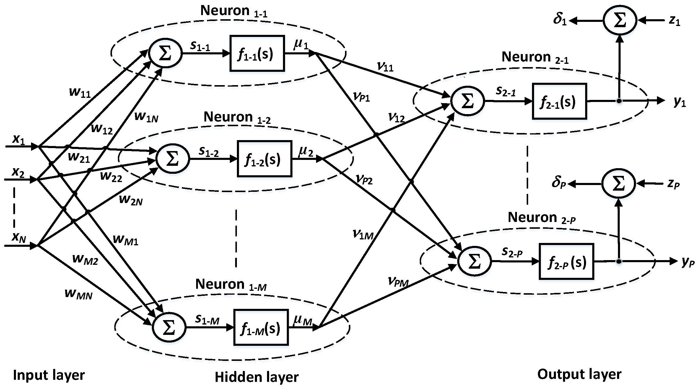
Hardware Implementation of the ANN

A review of the state-of-the art literature shows that multilayer backpropagation (BP) ANNs offer popular solutions for prediction problems. In the problem addressed in this paper, the amount of input data for such ANNs is relatively small and varies between 4 and 15, depending on the described solution. At the same time, the network should output one or several computed signals, each of which is a prediction of one type of pollution.

The BP learning algorithm is now new. One can also find its various hardware realizations, to mention only two of the newest ones [26,27]. In [26], for example, an analog voltage-mode CMOS-memristive BP learning circuit is proposed and implemented in the TSMC CMOS 180 nm technology. The authors of this work paid attention to the realization of basic components used in this circuit, such as sigmoid and tangent activation function, multiplying circuit, an amplifier, and analog switches.

In [27], nanoscale memristive devices have been used to support the design of the BP ANN. It is a hybrid CMOS-memristive convolutional computation system for on-chip learning. A modified backpropagation (BP) algorithm suitable for the proposed memristive neural networks is in this case applied to perform image convolution and recognition.

In our work, we propose another approach. Since the proposed BP architecture is going to become a component of a wireless sensor, a paramount feature is its implementation simplicity and strongly reduced energy consumption, so that the overall sensor does not require a complex power supply block. To make this possible, in our work, we propose such modifications to the learning algorithm so that it can be implemented using only elementary arithmetic operations.

3. Impact of Environmental Conditions on Prediction Results and Proposed Distributed Approach

When implementing the proposed system solution with the ability to predict changes in the level of pollution, the urban structure of the city should be also taken into account. There are many elements constituting a component of a given spatial arrangement of urbanized areas. From this article’s point of view, quite important are buildings and open areas. In cities, this depends, among other things, on dispersion conditions, i.e., spreading, taking into account various precipitation, temperature differences, or air mass movements. For example, large green spaces, such as parks or riverside boulevards, serve as “ventilating wedges”, contributing to the thinning of harmful substances in the air. Therefore, in these types of areas the level of pollution, temperature, or humidity will be different to the rest of the city. Wind speed may also be different, especially along watercourses; within such areas, there will also be other results of temperatures and humidity, which may affect the study of the level of pollution.

It is worth noticing that for similar values of T, RH, WS, WD, ${\mathrm{PM}}_{10}$ factors but for different environmental conditions, predicted pollution levels may differ significantly. Selected conditions that may affect the prediction process are briefly characterized below.

Geographical location of the city—is the factor related to the specificity of the place, which includes not only the structural arrangement, the nature of open spaces (especially green), but also the kind of microclimate of the place (climate zone), e.g., by the river or sea, etc. A tool such as a geographic information system (GIS) may prove helpful here.

Density and height of buildings,—also so-called aerodynamic roughness of the terrain, has a direct impact on ventilation abilities. The wind speed in the city is on average lower by 20% at night and 30% in the day. There may also be an increase in the wind speed in the city, which is the so-called tunnel effect (air flow in accordance with the street route).

The building dimensions are directly related to the exposure of the area to the sun (sunlight/shading), as well as the rate of heating and cooling. These are often the result of local traditions and climatic requirements.

The phenomenon of so-called urban heat islands—the air above the city center is warmer than outside the city, hence as it is lighter it rises and causes local pressure reduction, causing air suction from the areas surrounding the city. The formation of this phenomenon can be compounded by a large number of people and the emission of anthropogenic heat (other conditions will be e.g., in places of large crowds of people—e.g., at a stadium during a match, which will increase the air temperature); Here, the size and spatial structure of the city also matters, because low, not very compact buildings do not create urban heat islands.

However, equally important, in this context, seem to be such factors as the share of impervious surfaces, surface albedo, overall land use or the type and density of buildings, which may contribute to exacerbation or mitigation of the urban heat island phenomena.

Building geometry—is a factor that has an impact on the degree of inhibition of natural air movement in the city. This factor most strongly affects the nature of aerodynamic phenomena in cities, but it is difficult to predict and is associated with the scope of aerodynamics, and more precisely with fluid mechanics ((C)FD—(Computational) Fluid Dynamics). It can be assumed, however, that sudden gusts of wind in the city, in turn, occur e.g., in the vicinity of medium–high, high and high-rise buildings (at walls and in the corners of buildings);

Roads and streets—due to their function and the vehicles moving on them, are one of main sources of pollution, and also depend on the type of surface of the space (the problem of possible sealing of the ground).

Specificity of tightly built-up urban interiors—is also one of main factors influencing the pollution level. Streets or squares/courtyards, especially when the distance between buildings is less than 1.5 times their height, may be a phenomenon of air stagnation or air circulation without replacement. In such spaces, there are certainly other local conditions (on a micro scale—within e.g., places with residual odors, overheating in summer at high temperatures, etc.). This is regarding the so-called Local Climate Zones (LCZ), which were selected and developed for selected cities in Canada [28]. These local climate zones set conditions on a small scale due to typically urban features, including the share of impermeable surfaces, surface albedo, general land use, or the type and density of buildings. They are affected by factors such as the exposure of the area to the sun (sunlight/shading), as well as the rate of heating and cooling.

All the factors described above change daily. They also change throughout the day, but also depend on the season. In some seasons, the relative temperature difference between the city center and its suburbs increases due to the heating of apartments. These changes also take place in different spaces (local zones) and have a different course. Buildings in the center are sometimes higher and denser (which is characteristic of the promoted “compact city”), and its organization and shape have a direct impact on local conditions and air quality [29].

From the point of view of urban planning, the most important thing is to create healthy and comfortable living spaces. Due to many years of spatial development and the flourishing of transport (including individual transport), they are an excellent example of a living space with a rich cultural and economic offering, and at the same time with a deteriorating quality of life caused by harmful and onerous factors. These include smog (air pollution), noise, traffic jams, and shrinking green areas. Therefore, it is extremely important to counteract the aforementioned deterioration of living conditions in cities, especially regarding air quality.

The functions often arranged in a city and the transport network necessary for operation are among the main sources of air pollution in the city. However, the aforementioned development of buildings in so-called downtown contributes to the “stopping” of these harmful substances, additionally hindering their removal (blocking the ventilation of cities).

Currently, researchers focus most often on attempts to eliminate the sources of smog in cities. The most common is the reorganization of urban transport, restricting the movement of especially passenger cars, or informing citizens about the air quality in specific zones, encouraging them to be active outdoors or stay at home, respectively [30]. Various, most often technological solutions (e.g., Intelligent Transport System, electric/biofuel vehicles, etc.) or legal solutions (bans, restrictions, penalties, etc.) serve this purpose. Considering the above problem, it is extremely important to take action on various levels of shaping and functioning of modern cities. Some of them require a longer time to implement (e.g., increasing the biologically active surface, planting trees, etc.). Other measures can be implemented in cities almost immediately, such as a proposed pollution prediction system monitored by a network of air sensors.

To sum up, within the structure of a modern city it is difficult to find a small group of representative urban zones, in which a model prediction process could be carried out. In practice, each sensor in the city responsible for prediction should be trained based on an individual dataset, consisting of a specific vector of the input signals as well as a desired response of the ANN. Current solutions are able to provide only average responses in a specific area. Taking this into account, in the next section we present a solution in which such individual training sets are created automatically, without the need to contact the base station of the wireless sensor network (WSN).

4. Materials

The proposed system is being developed at several levels. On the one hand, these are simulations at the model level, in which the influence of the values of selected parameters on the accuracy of mapping the activation function using the proposed approximating function is examined. These tests are performed in the Matlab/Octave environment. Based on these results, a transistor-level implementation of such a function with the possibility of reconfiguring its parameters was proposed and verified in the Hspice simulation environment. Subsequently, a prototype chip was designed containing selected components of the neural network, which was verified by measurements.

4.1. Octave/Matlab Software Development Environment

One of the solutions proposed in this work is an approximation function that replaces nonlinear activation function and its derivative, which is complex in the case of hardware implementation. An algorithm responsible for determining optimal parameters of the activation function has been realized in the Octave/Matlab environment. It is used to minimize errors made during the approximation, depending on selected values of other parameters. At the same time, the program allows the obtaining of a relatively simple representation of the computed parameters in the fixed-point notation. This is important from the point of view of such hardware implementation, in which particular neurons in the ANNs work in parallel. In the proposed approach, it is assumed that the parameters of the approximation function may be adjusted during the learning process, based on the quality of the learning process of a given ANN.

4.2. Chip Design and Verification

A prototype chip containing selected components to be used in the proposed solution has been designed in the CMOS 130 nm technology. The chip was designed and verified in the Cadence environment, with the use of such modules as Virtuoso, Layout-vs. Schematics (LVS), Spectre simulator, etc. A thorough corner analysis has been performed under varying process, voltage and temperature (PVT) parameters. Comprehensive transistor-level simulations were carried out for the supply voltage varying between 0.8 and 1.2 V, temperature varying between −40 and +140 ${}^{\circ }$C degrees, for typical, slow and fast transistor models.

The chip was tested using a dedicated measurement PCB equipped with, among others, an on-board programmable device XC9572XL (Xilinx), a cross-over matrix in the form of a CPLD (complex programmable logic device) circuit, I/V and V/I converters, and buffers for analog lines.

The PCB cooperated with the measurement equipment, which included a MyRio 1950 measuring card that operates under the control of the LabView (LV) environment, a programmable, precise DC power supply, and Tektronix oscilloscopes and generators.

5. Methods

In this section, we provide a brief description of design methodology related to the proposed solutions. First, we deal with solutions for the overall network of air pollution sensors. Then we focus on the neural network used in the prediction process.

5.1. Proposed Distributed Prediction Tailored to Local Conditions

Based on the considerations presented in previous sections, several general conclusions can be drawn. In many state-of-the-art works presented in Table 1, the ANN with the BP learning algorithm has been successfully used. Another conclusion is that in most cases the used learning dataset was relatively simple, being composed of basic weather conditions. On the other hand, as discussed above, it may be beneficial when other environmental conditions are also included in the learning dataset, especially when an accurate predictive map of air pollution with high spatial resolution is desired.

In our opinion, however, adding urban parameters to the learning dataset is associated with several disadvantages. First, such data must be collected in advance. This is an expensive and logistically challenging task, taking into account an assumed large number of sensor nodes installed in the city.

Secondly, the parameters associated with the environment of the sensor, including its geographical location, are very diverse and complex. Describing them using only parameters such as BH and SW (see Table 2) may be too simplistic. In practice, it can also be problematic to build an appropriate (comprehensive) learning set containing such data. In the case of the ANN trained in a supervised mode, specific input patterns should be matched by a specific correct output. Such results must be determined in advance. The use of a single dataset, even limited to a given geographical area, in practice means that ultimately all sensors will be equipped with the ANN with the same weight values. In this situation, particular sensors can work in a sub-optimal way, as discussed above.

Taking the above into account, in this work, we propose a different approach, in which the learning process is carried out for each of the sensors independently, in parallel from the point of view of the overall WSN. We propose to equip all sensors in the WSN with ANNs realized as specialized integrated circuits that may be integrated with other components of such devices, as described in our previous work [31]. This allows particular ANNs to be trained based on datasets composed of local conditions in the city. In this approach, even if the training set is composed only of parameters related to weather conditions, taking into account that these are data from the immediate vicinity of the sensor, these parameters are sufficient to train the ANN. In other words, local weather conditions and how they affect future air pollution levels reflect the local environment conditions described in Section 3.

One of the important features of the proposed solution is that we do not need a single universal learning dataset, containing parameters related to the urban environment. In this case, personalized learning sets for particular sensors are directly available throughout measurements of external pollution and weather signals.

Conceptually, the learning process of the ANN proceeds as follows. In a given (current) iteration k, the ANN receives a training pattern $X^k$ consisting of actual (measured) samples of particular input signals, $x_1,x_2,\cdots ,x_N$ shown in Figure 1, as well as a resultant value expected at the output of the ANN. In the case of the prediction system, the expected output value is an expected pollution level after subsequent L samples (prediction time horizon), $y^{k+L}$. Based on these signals, the ANN calculates the estimate of this signal, ${\widehat{y}}^{k+L}$ and compares it with a real signal $y^{k+L}$. The difference between these signals, $\delta$, is used to adapt the weights of the neurons in the ANN. The detailed learning process of the ANN is discussed in the next section.

The real pollution level (after the L samples) is however not known, which is the main drawback of a conventional approach. To work around this problem, we propose a different solution. In this case, the values of the input signals (weather conditions and actual pollution levels) measured in subsequent moments, k, are stored in an internal memory of the sensor and held for the next L samples. In particular iterations, k, the device additionally measures actual values of the $y_{\mathrm{MEAS}}^k$ signal. The $y_{\mathrm{MEAS}}^k$ signal is the value expected at the output of the ANN, looking from the point of view of the iteration $k-L$. Thus, in a given iteration k, the ANN is trained with the pattern $X^{k-L}$ that contains values of the input parameters from before L samples, as well as the actual pollution level $y_{\mathrm{MEAS}}^k$. Based on them, it calculates the estimate of this signal, ${\widehat{y}}_{\mathrm{MEAS}}^k$. The difference between these signals is then used to adapt the weights of neurons. The difference between the conventional and the proposed approach is illustrated in Figure 2.

In this approach, the prediction is delayed by L samples, but only during the training phase. One of main advantages of the proposed solution is that the ANN in a given sensor has access both to locally measured input signals, as well as to ideal (locally measured) expected values y. During the training phase, when the sensor is not used to create the map offered on-line to the users, the delay does not impact the learning process itself and the final results. After completing the learning process, when the samples of the $y_{\mathrm{MEAS}}$ signals are no longer necessary, the network can be switched to actual values of the $X\left(k\right)$ pattern.

This approach offers several advantages:

• Many input parameters are not needed, and the sensor itself measures those that are required.
• Implementing the learning process of the ANN directly in the sensor device limits the amount of data that in a conventional approach would have to be exchanged between the sensors and a base station.
• It leads to a scalable and flexible system. Since the time-consuming learning process is performed in parallel in all sensors mounted in the urban infrastructure, the required computation power of the base station is almost independent of the number of the sensors.
• The ANNs in particular sensors do not need to be pre-programmed before their installation in the urban infrastructure. Each sensor has an equal structure and is equally initialized (weights values). This facilitates the process of their production, installation and maintenance.

To make the realization of this idea possible, it is necessary to develop the ANN as a specialized integrated circuit and integrate it with other components of the sensor. We have been dealing with the implementation of hardware ANNs in the CMOS technology for many years [32,33,34]. Thus, many building blocks of such ANNs have been already verified earlier and we do not need to build and test the overall ANN from scratch.

5.2. Proposed Modifications of the Learning Algorithm and Structure of the ANN

A block diagram of the BP ANN, with N inputs, a single hidden layer composed of M neurons and the output layer composed of P neurons, is shown in Figure 1. In the learning process of the BP ANN, particular iterations are divided into two phases. First, the NN computes an error $\delta$ based on the input data X. This error is determined separately for each neuron in the output layer. The error is defined as a difference between an expected value, d, and the output signal from a given output neuron, y. For a selected 1st neuron, it may be expressed as follows:

$${\delta }_1^k=z_1^k-y_1^k.$$

(1)

For the ANN shown in Figure 1 the output signal ${\mathit{y}}_1$ equals:

$$y_1^k={\vartheta }_{11}^k·{\mu }_1^k+{\vartheta }_{12}^k·{\mu }_2^k+\cdots +{\vartheta }_{1M}^k·{\mu }_M^k,$$

(2)

where:

$${\mu }_m^k=f_{1m}(x_1^k·w_{m1}^k+x_2^k·w_{m2}^k+\cdots +x_N^k·w_{mN}^k)$$

(3)

for $m=1,\cdots ,M$.

The w and $\vartheta$ factors in Equations (2) and (3) are weights of neurons in the 1st and the 2nd (hidden) layer of the ANN, respectively. The first index denotes a given output neuron, while the second index represents a given network input.

The errors ${\delta }_1$ … ${\delta }_M$, computed for particular output neurons, are used to compute the errors for the hidden layers, as shown below, for an example case of the first output neuron:

$${\delta }_{1m}^k={\delta }_1^k·{\vartheta }_{1m}^k+....+{\delta }_P^k·{\vartheta }_{Pm}^k$$

(4)

The described computation chain is the error backpropagation core procedure. In the following step, based on the computed errors, the ANN triggers the adaptation process of the weights of its own neurons, according to Formulas (5) and (6), for the first and the second layer, respectively. These formulas are given for selected neurons ${\mathrm{Neuron}}_{1-1}$ and ${\mathrm{Neuron}}_{2-1}$, for $n=1\cdots N$ and $m=1\cdots M$, as follows:

$$w_{1n}^{k+1}=w_{11}^k+\eta ·{\delta }_{11}^k·x_n^k·\frac{d{f}_{11}\left(s\right)}{ds}$$

(5)

$${\vartheta }_{1m}^{k+1}={\vartheta }_{1m}^k+\eta ·{\delta }_{21}^k·{\mu }_m^k·\frac{d{f}_{21}\left(s\right)}{ds}$$

(6)

In the formulas above, the $\eta$ factor is the learning rate. It is set to the value close to 1 at the beginning of the learning process, and then it diminishes toward 0. When it reaches 0, the learning process is complete.

In the proposed approach, the sigmoid activation function, $f\left(s\right)$, has been applied based on a hardware implementation described in [35]. This function is described as:

$$f\left(s\right)=\frac{1}{1+e^{-\beta ·s}}$$

(7)

Derivation operation of this function, $\frac{df\left(s\right)}{ds}$, present in Equations (5) and (6), can be expressed as follows:

$$\frac{df\left(s\right)}{ds}=\beta ·f\left(s\right)·[1-f\left(s\right)]$$

(8)

Taking (8) into account, (5) and (6) can be expressed respectively, as follows:

$$w_{11}^{k+1}=w_{11}^k+\eta ·{\delta }_{11}^k·x_1^k·\beta ·f\left(s\right)·[1-f\left(s\right)]$$

(9)

$${\vartheta }_{11}^{k+1}={\vartheta }_{11}^k+\eta ·{\delta }_{21}^k·{\mu }_1^k·\beta ·f\left(s\right)·[1-f\left(s\right)]$$

(10)

After the adaptation, the output signals for all neurons are computed with the use of Equations (2) and (3).

As can be seen in (2), (3), (9) and (10) above, the learning process of the BP ANN can be expressed with the use of such mathematical operations as summing, subtracting, multiplying and determining the value of the sigmoid function, expressed by Equation (7). We propose a substitution of the last two terms in Equation (10) with a new $\Lambda \left(s\right)$ function, expressed as follows:

$$\Lambda \left(s\right)=f\left(s\right)·(1-f(s\left)\right)$$

(11)

As a result, Equations (9) and (10) can be rewritten respectively, as follows:

$$w_{11}^{k+1}=w_{11}^k+\eta ·{\delta }_{11}^k·x_1^k·\beta ·\Lambda \left(s\right)$$

(12)

and

$${\vartheta }_{11}^{k+1}={\vartheta }_{11}^k+\eta ·{\delta }_{21}^k·{\mu }_1^k·\beta ·\Lambda \left(s\right)$$

(13)

In the proposed approach, the $\Lambda \left(s\right)$ function is realized as a single block and requires only simple arithmetic operations, as described below. The $f\left(s\right)$ and $(1-f(s\left)\right)$ terms, as well as the resultant $\Lambda \left(s\right)$ functions, for an example case of $\beta =1$, are shown in Figure 3.

Proposed Hardware Implementation of the Learning Algorithm of the ANN

The implementation of Equation (12) requires simple arithmetic operations (multiplication, summation and subtraction). This is because the $\Lambda \left(s\right)$ function in the proposed approach is approximated with the use of a polyline. The polyline is composed of line segments, each being expressed by a pair of a slope and an offset in the vertical axis. The values of these two factors are stored in a look-up table (LUT). The size of the LUT depends on the number of segments of the polyline. However, since the $\Lambda$ function is symmetric across the vertical axis, the size of the LUT may be reduced by half.

The key issue here is how LUT indexing is implemented. We propose a solution, in which the indexing operation, as well as subsequent computing of the output of the $\Lambda \left(s\right)$ function, is performed fully asynchronously in a single step, with the use of a circuit shown in Figure 4. The circuit is very fast, as shown in the next section.

The input signal, s, of the $\Lambda \left(s\right)$ function is a multi-bit signal, with the number of bits being one of the parameters here. In the proposed implementation, the number of segments is one of the powers of 2, which simplifies the hardware implementation.

Two calculation paths can be seen in Figure 4. The signal s is fed to both these paths, where it is divided into two components by means of the signal and the address masks. Both the mask blocks are only composed of a few AND logic gates. The most significant bits of the signal s are separated from this signal with the address mask. The resultant signal is used directly for indexing the LUT. The ${\mathrm{M}}_{\mathrm{A}}$ signal, fed to the address mask, determines the number of MSBs used for addressing the LUT, and thus directly specifies the number of segments of the polyline. The remaining bits are extracted from the input signal by means of a signal mask ${\mathrm{M}}_{\mathrm{S}}$. The output from this mask is an offset along the horizontal axis with respect to the beginning of a given segment. In response to a given address signal, A, the LUT returns the values of the slope and offset. At the same time, in the neighboring path, the output from the signal mask is first multiplied by a given value of the slope, and then the offset is added to the results of this multiplication. In practice, the ${\mathrm{M}}_{\mathrm{S}}$ mask is equal to the negated value of the ${\mathrm{M}}_{\mathrm{A}}$ mask. For example, for a 12-bit signal s, if ${\mathrm{M}}_{\mathrm{A}}=\mathrm{B}111110000000$ then ${\mathrm{M}}_{\mathrm{S}}=\mathrm{B}000001111111$. As a result, the number of segments equals 32, while the signal in each segment varies from 0 to 127.

The values of the slopes and the offsets stored in the LUT are computed with the use of a program written by us. This tool for a given number of segments and a given range of the s signal minimizes the errors between the ideal and the approximated values of the $\Lambda$ function. The values of these two factors are represented by fixed-point numbers, to simplify the multiplication and the summing operations in the hardware.

In this approach, the multiplication operation is performed using a binary-tree (parallel) multiplier, composed of asynchronous multi-bit full adders (MBFAs). This kind of multiplier, for an example case of 8-bit input signals, is shown in Figure 5. Its application allows the performance of all multiplication operations in the chain in a single step, without using a clock generator. This is one of the important advantages of the proposed approach.

In Equations (12) and (13) there is a series of multiplication operations. However, one can notice that $\eta$ and $\beta$ factors are constant for many iterations of the learning process. Since the slopes stored in the LUT are also constant values, then all these terms may be combined together and stored in the LUT. As a result, Equations (12) and (13) may expressed as follows:

$$w_{11}^{k+1}=w_{11}^k+({\delta }_{11}^k·x_1^k·{\mathrm{O}}_{\mathrm{S}}·\mathrm{B}\left(\mathrm{s}\right))+\mathrm{Off}\left(\mathrm{s}\right)$$

(14)

$${\vartheta }_{11}^{k+1}={\vartheta }_{11}^k+({\delta }_{21}^k·{\mu }_1^k·{\mathrm{O}}_{\mathrm{S}}·\mathrm{B}\left(\mathrm{s}\right))+\mathrm{Off}\left(\mathrm{s}\right)$$

(15)

where $B\left(s\right)$, given below, is a constant factor for a larger number of iterations k.

$$B\left(s\right)=\eta ·\beta ·\mathrm{SL}\left(\mathrm{s}\right)$$

(16)

6. Results

6.1. Results at the Model Level

The process of approximation for the selected resolutions of the s signal, selected ranges of this signal, as well as selected values of the masks ${\mathrm{M}}_{\mathrm{A}}$ and ${\mathrm{M}}_{\mathrm{S}}$ are shown in Figure 6, Figure 7 and Figure 8.

Figure 6 presents the approximation of the $\Lambda \left(s\right)$ function for the resolution of the input signal s of 8-bits, varying in the range from −10 to 10, for several numbers of the MSBs. Diagrams (a,b) show results for 3 bits (8 segments), diagrams (c,d) show results for 4-bits (16 segments), while the (e,f) diagrams illustrate the case of 5 bits (32 segments). Particular diagrams illustrate the approximation process for selected values of the $\beta$ factor.

In Figure 7 the results are shown for the resolution of the s signal of 12-bits, for a constant number of segments (64) but for different values the range of the signal s.

Finally, Figure 8 presents similar results to Figure 6 but for 10 bits of the signal resolution, in the range of (−10, 10) for larger numbers of segments.

6.2. Results at the Hardware Level

The circuit components responsible for the described operations have been realized in a prototype chip realized in the CMOS 130 nm technology.

Selected simulation results illustrating the behavior of the proposed approximation circuit are presented in Figure 9. The results are provided for the resolution of the s signal of 14 bits, with 6 MSBs used to determine the address of the segment of the polyline. The signal s varies in the range −10 to 10, with this range being superimposed on $2^{14}$ = 16,384 levels (fixed points numbers) of the signal that represents the s signal in the transistor-level implementation. For such settings, the input range is divided into 64 segments, while each segment contains 256 samples (8 bits). In the presented case the slopes in the LUT are stored on 8 bits, while the offsets are on 20 bits. The aim of the presented results is to illustrate the dynamic properties of the circuit, i.e., delays that translate into data rate.

In the presented case, an example value 6811 (B01 1010 1001 1011) of the s signal has been split into the address ${\mathrm{O}}_{\mathrm{A}}=B011010$ (26) and the signal ${\mathrm{O}}_{\mathrm{S}}=B10011011$ (155). The signal ${\mathrm{O}}_{\mathrm{S}}$ is counted from the beginning of a given slot (segment), indicated by ${\mathrm{O}}_{\mathrm{A}}$. Since the LUT is indexed from 0 to 63, the input value is in the 27th slot. For this slot, the values of the slope and the vertical offset equal 238 (B1110 1110) and 247,808 (B0011 1100 1000 0000 0000), respectively. The resultant output of the $\Lambda \left(s\right)$ approximation function equals 284,698 (B0100 0101 1000 0001 1010). This value can be reduced by dividing it by one of the powers of 2, using a simple bit-shift circuit. The bit-shifting operation is important because the levels of the output signal should be matched with other ANN components.

The described signals are presented in the top three panels of Figure 9. The third panel provides details that allow the assessment of the maximum data rate (17 ns for this example case). The bottom panel illustrates the supply current $I_{\mathrm{DD}}$ drawn from the supply voltage of 1.2 V during the computation of a single output value. An average value of this current within the mentioned period of 17 ns does not exceed 3 mA, so the consumed energy equals approximately 41 pJ per a single computed value.

7. Discussion

7.1. Discussion of the Proposed Learning Method

In our work, we present investigation results of one of the important steps of a larger project that aims at building autonomous sensors with the function of the prediction of air pollution levels. The sensor itself is a complex device. For this reason, to make a final design successful, a prior design of its particular components is a mandatory phase. We already designed and tested most of these blocks as prototype chips. They include, for example, a low-power, low-chip-area analog-to-digital converter (ADC). We also designed an on-board algorithm, whose role is to control the timing of the wireless transmission of collected and processed data to a base station [31]. In our previous work, we showed that the periods between consecutive data transmission sessions may be variable and dependent on the rate of signal change at the sensor input.

One of the more important aspects is the verification of the prediction process in a real environment. At this stage of the project, it is not yet possible to present such results, since full sensors are still at the development stage. However, at this stage we can rely on prediction results obtained by other research teams that have already explored predictions of air pollution using various ANNs, based on real-world data. In our work, we refer to these works, treating them as a starting point for the development of the proposed concepts.

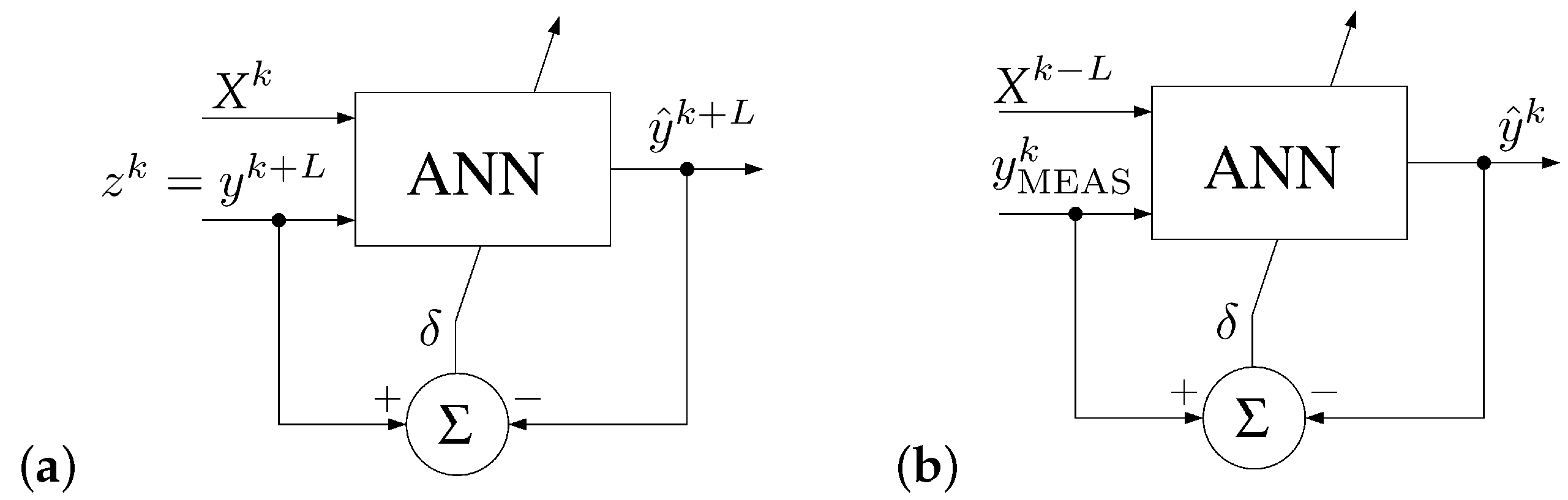
A general training scheme of the ANN is in the proposed case similar to that already reported in the literature. The key aspect of our concept, however, is the introduction of a time delay during the learning phase. Thanks to this, we do not have to create the training dataset in advance. In the conventional approach, it is necessary to prepare such training sets before starting the learning process. Such sets are composed of two groups of data. One of them is input factors that include, for example, quantities describing weather conditions as well as current pollutant levels. The second group provided to the inputs of the ANN is expected (predicted) values of pollution levels after a given time horizon. In other words, based on the input data collected at $t_1=t_0$, where $t_0$ is the present moment of time, the ANN is going to find out what levels of pollution are expected in the future, at $t_2=t_0+{\Delta }_T$, where ${\Delta }_T$ is an equivalent of variable L in Figure 2. The ${\Delta }_T$ is the time horizon for the prediction process.

In the case of the concept proposed by us, the moment of collecting the input data and the moment for which we determine the expected values are also separated by the time interval ${\Delta }_T$. As a result, the learning process itself is similar to the conventional approach. However, we have introduced a modification in which the network is trained based on data collected in the past, at the moment $t_1=t_0-{\Delta }_T$. These data are sampled and stored for given time intervals equal to a sampling period in the memory of the sensor device. At the inputs of the ANN, we also provide the expected value, but in this case this value is also measured by the sensor itself, at the time $t_2=t_0$. To summarize:

In the conventional approach, one can show that $t_2-t_1=(t_0+{\Delta }_T)-\left(t_0\right)={\Delta }_T$.

In the proposed approach $t_2-t_1=\left(t_0\right)-(t_0-{\Delta }_T)={\Delta }_T$.

Thus, as can be seen in both cases, $t_2-t_1={\Delta }_T$, which means that the learning process will be similar (only shifted in time), and therefore, at this stage of the project, in our opinion it is sufficient to rely on the results of tests carried out in a conventional manner by other teams.

Thanks to the introduced ${\Delta }_T$ delay, the sensor itself can measure both the input values and the expected value, which is the key advantage here. This strongly simplifies the training process of all wireless sensors mounted in a given area of the city. Each sensor itself creates its own training set along with the expected values. In this way, the resultant training sets are fitted to conditions prevailing in particular points of the city. Additionally, during the training phase of the ANN, there is no need to provide an external training set to particular sensors via the base station. In this sense, the sensors may work as autonomous units. Since the communication with the base station may be limited in this phase, the consumed energy may also be reduced.

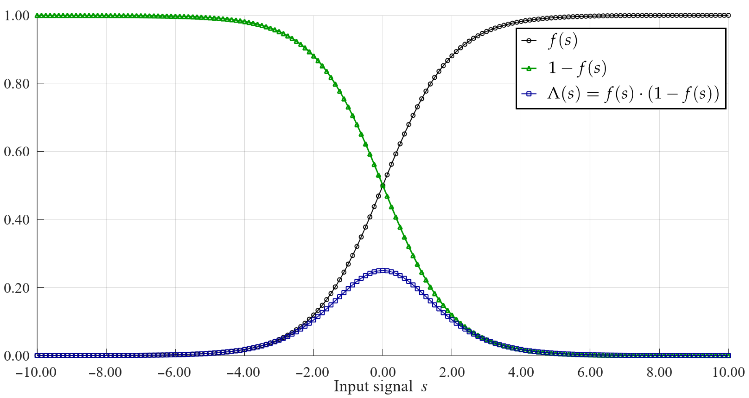
7.2. Results at the Model Level

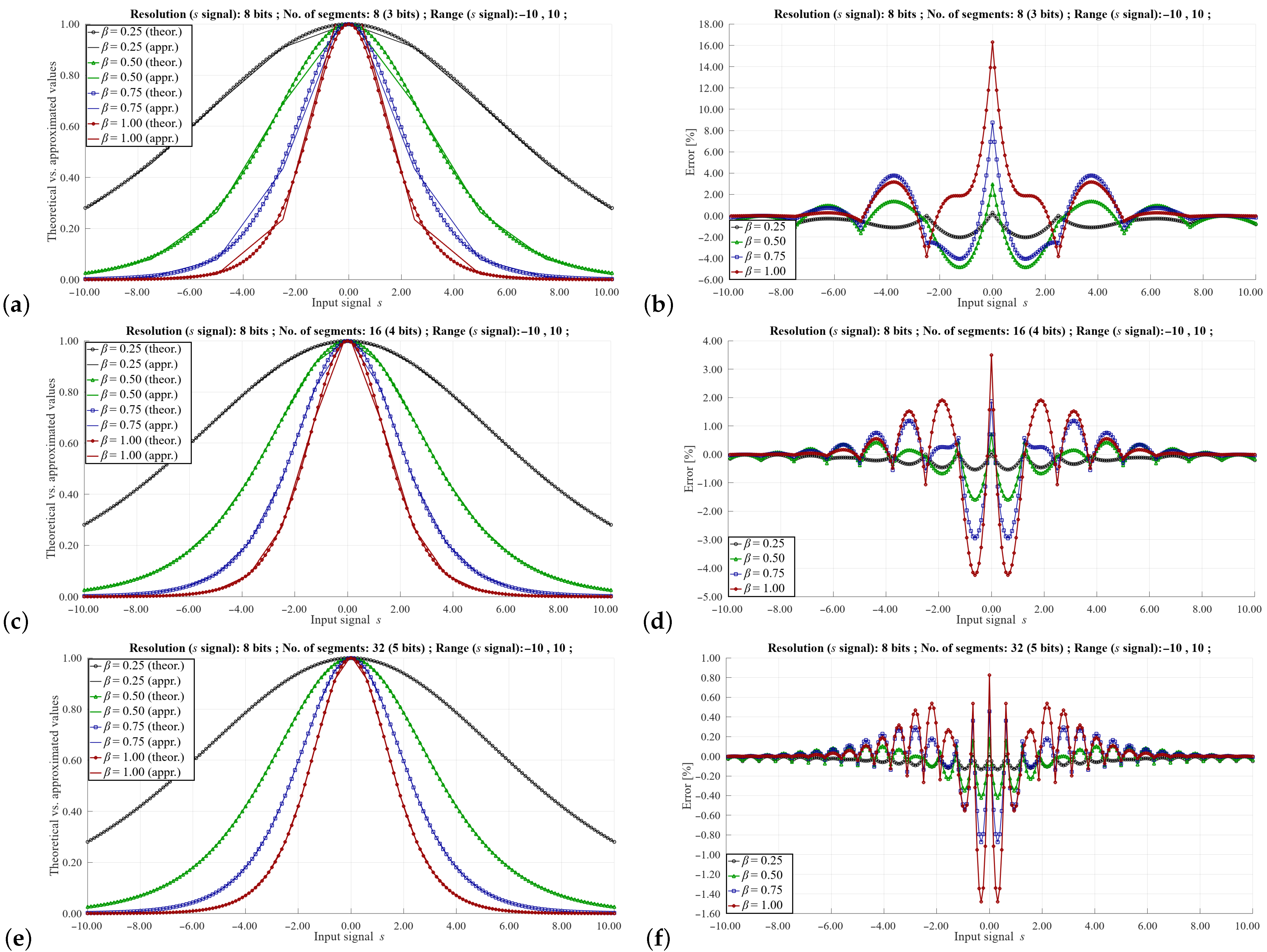
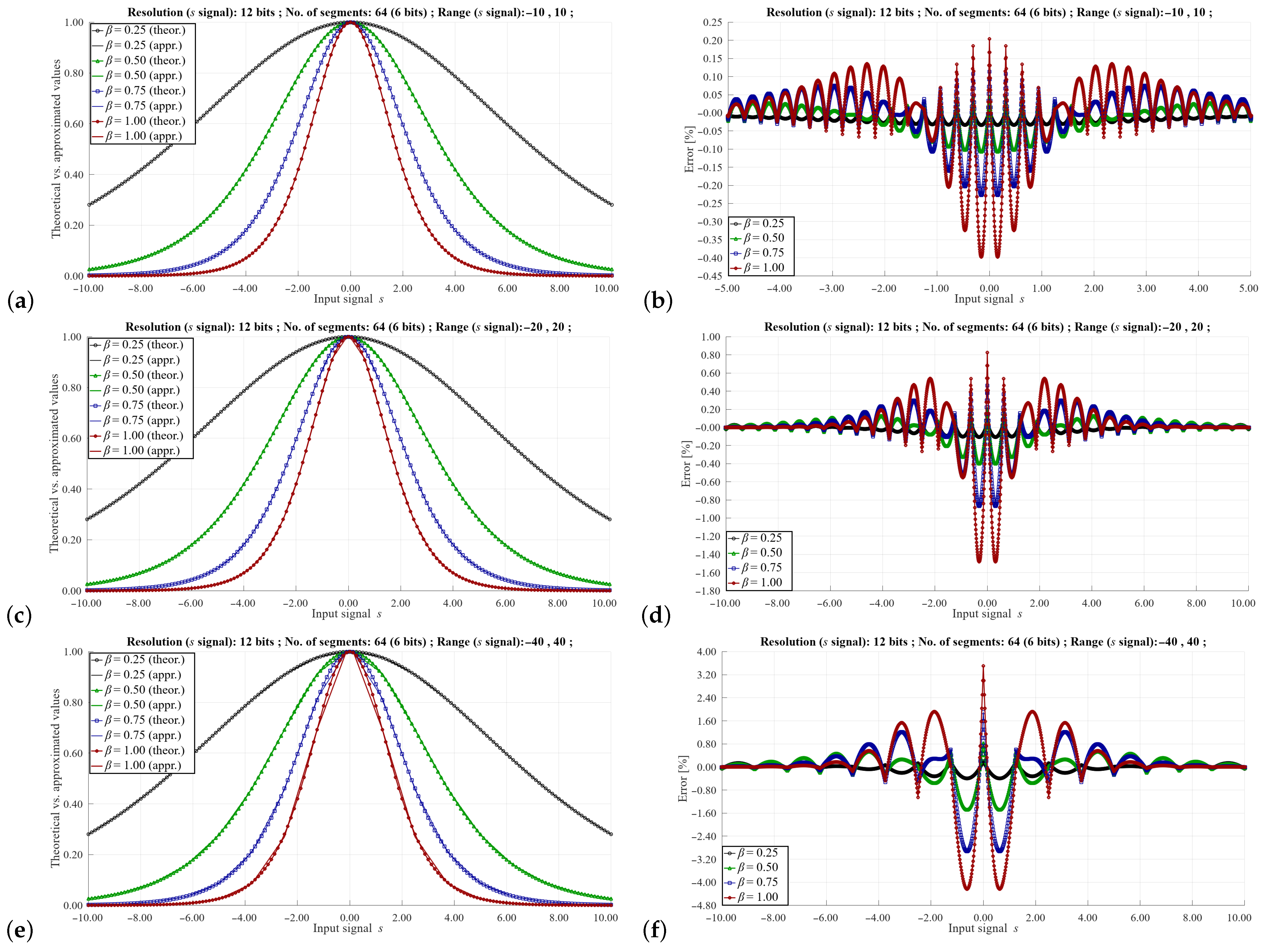
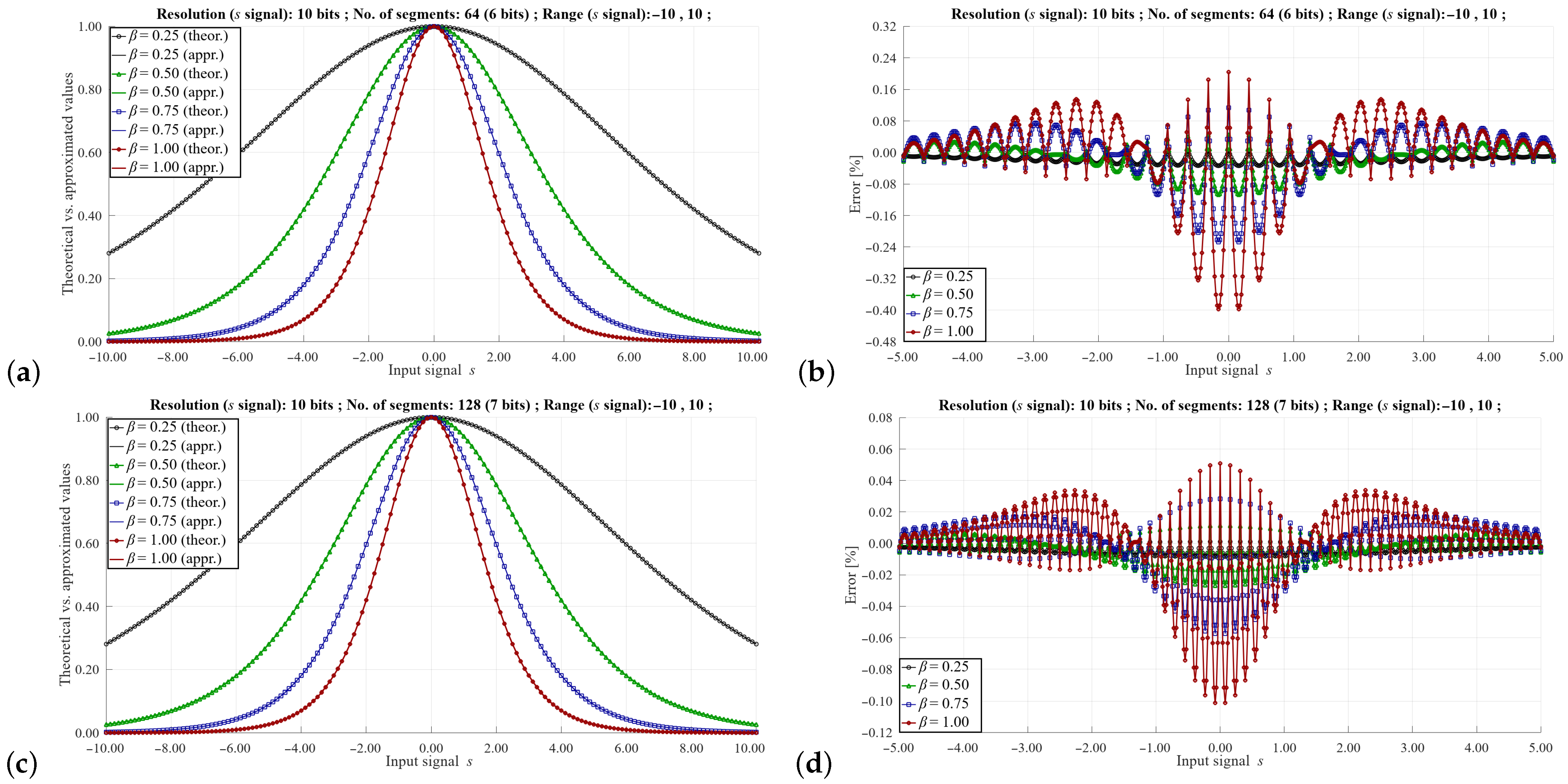
Figure 6, Figure 7 and Figure 8 show the approximation results for selected parameters described in the previous section. These parameters include the signal resolution s, the range of this signal and the values of the masks ${\mathrm{M}}_{\mathrm{A}}$ and ${\mathrm{M}}_{\mathrm{S}}$. As can be seen, the maximum value of the approximation error can vary to a large extent depending on these parameters. As would be expected, the highest error values occur with a small number of segments and a relatively large signal range of the s signal. In such cases, the error can reach even a dozen %. However, such signal resolution values are not used in a real implementation of the training algorithm, as this would distort the learning process of the neural network. In practice, higher signal resolutions are used. For a larger number of segments and higher signal resolutions s, it is possible to obtain a maximum error of 0.5–0.1%, which is sufficient to correctly reproduce the learning process of the ANN.

One of the advantages of the proposed solution is the ease of controlling the basic parameters of approximation using the values of masks ${\mathrm{M}}_{\mathrm{A}}$ and ${\mathrm{M}}_{\mathrm{S}}$, as well as appropriately selected values of the slopes and the offsets stored in the LUT. Since the slope and offset values are fixed-point numbers, it is not possible to directly compare the approximation results with the theoretical values. For example, in the case shown in the Figure 7, the value of the largest slope equals 255 (8 bits). Thus, to enable a direct comparison with the theoretical waveform, we have normalized the approximated waveforms to fit it to the theoretical case. In a real implementation, the normalization may be performed by a division operation, by a factor being one of the powers of 2, so a simple bit-shifting operation may be applied for this purpose.

Observation of the results shown in Figure 7 lead to the conclusion that the range of the signal s must be selected very carefully. If a larger signal resolution is required, one can apply a solution, in which the sizes of particular segments are not equal, being matched to the variability of the slope of the $\Lambda \left(s\right)$ function. In this case, to properly index the LUT, variable mask values are needed depending on the value of the signal s.

Comparing the results shown in Figure 7a,b and Figure 8a,b, it can be seen that with a given value of the range of the signal s and the same number of segments, the approximation errors are similar. This fact simplifies the programming of the LUT depending on the resolution of the s signal. In this case, the values of the slopes and the offsets are the same.

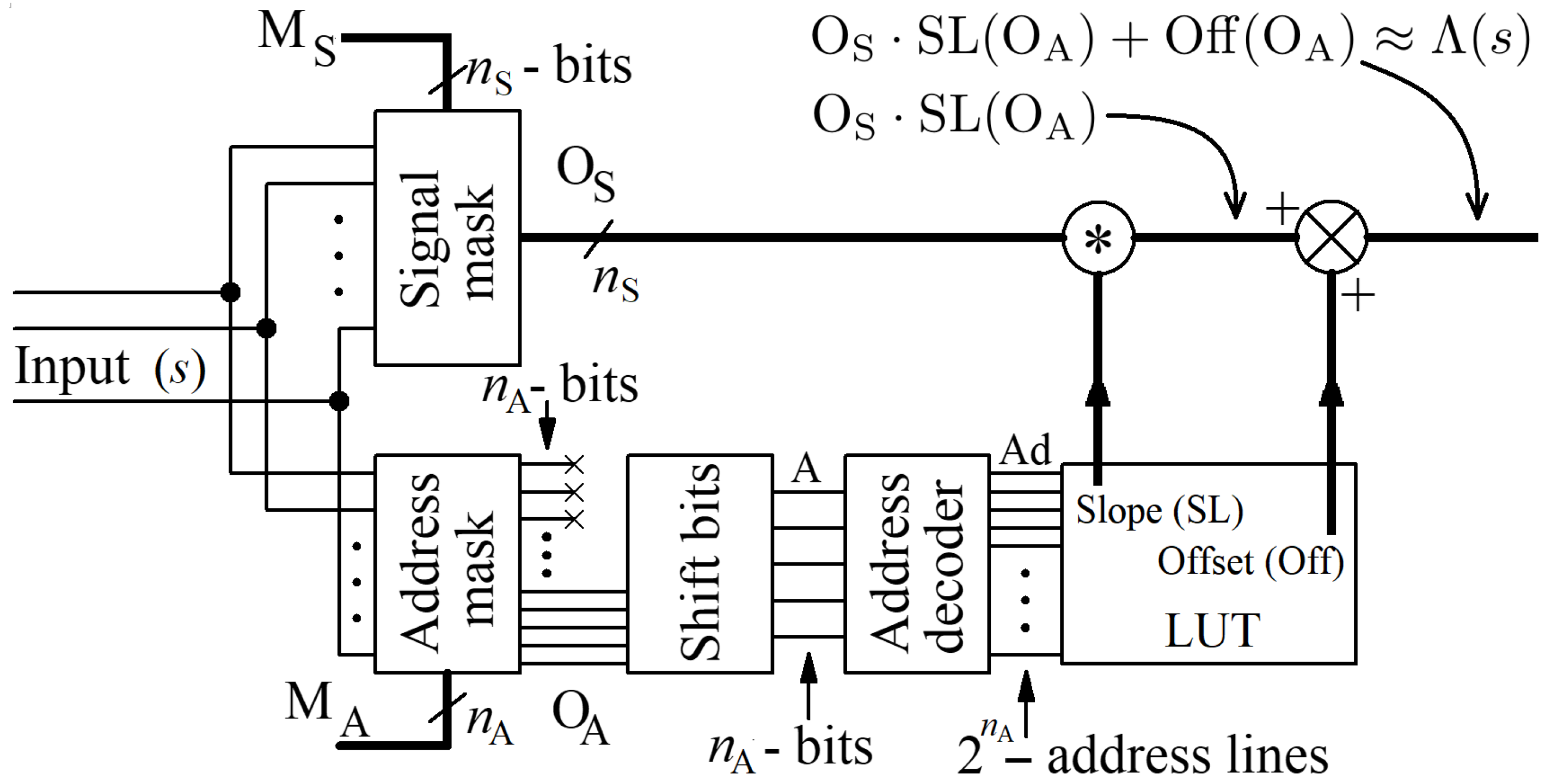
7.3. Results at the Hardware Level

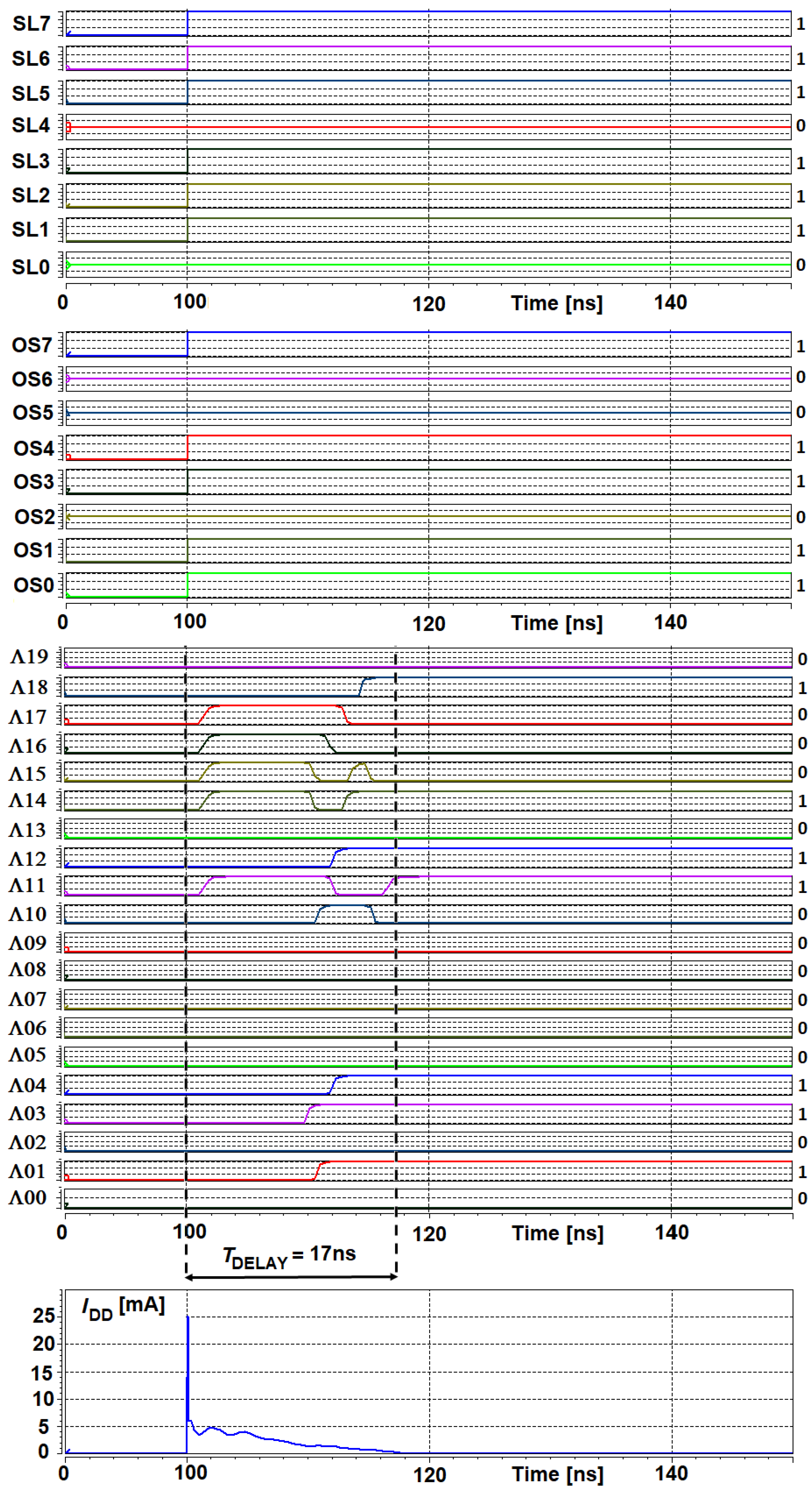
Figure 9 presents selected results at the transistor-level simulation of the proposed approximation circuit, shown in Figure 4. The input value (6811) has been selected so that the proposed circuit operates near the worst conditions. In this case, both the slope and the offset have values close to maximum levels stored in the LUT. This makes the delay time shown also close to the worst-case scenario.

The circuit shown in Figure 4 operates fully asynchronously. The asynchronous work is here understood in such a way that there is no need for an additional clock that sequences the computations at particular stages. After feeding the circuit with a new input signal sample, the result is ready after the time resulting only from delays introduced by particular digital elements and larger combination components. Thanks to this, several key features were achieved. They include simple structure, large data rate and low energy consumption per single signal sample.

In the proposed circuit, in the first step, the input signal is divided into two components using the address and the signal masks (complementary to each other). The masks are built as a single layer of AND logic gates working in parallel. Thus, the masks introduce a delay not exceeding 0.1 ns in the CMOS 130 nm technology.

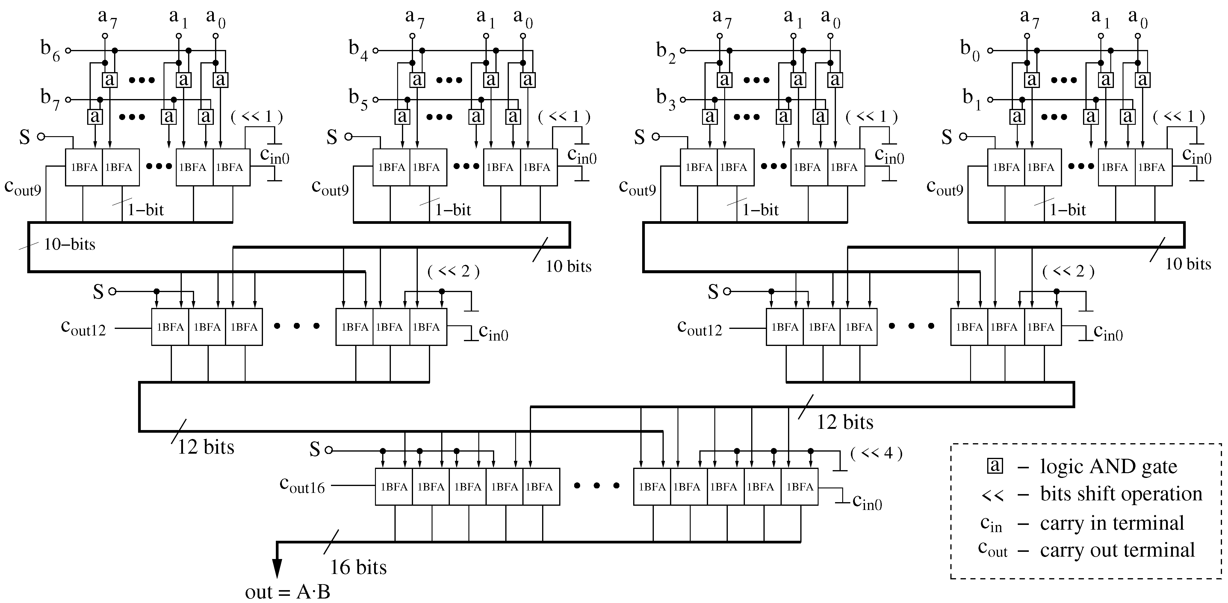
The multiplier block is built based on a binary tree consisting of asynchronous multi-bit full adders (MBFA). The delay introduced by this circuit depends, to a relatively small extent, on the resolution of the multiplied signals. When multiplying two 8-bit numbers, the tree consists of three asynchronous layers. If we increase the resolution to 16 bits then the number of layers only increases by one. As a result, the delay introduced by this block increases moderately with the resolution of the processed signals.

At the last stage of the signal processing chain, an additional summing circuit is used, whose structure depends on the resolution of the signals at the input of the multiplier. For the resolution of 8 and 16 bits, 17 and 33-bit MBFAs are used, respectively. One can also use a bit-shift block, to cut-off a given number of least significant bits (LSB), to normalize the signal at the output of the overall circuit.

The assessment of the circuit performance has been performed for the process, voltage and temperature (PVT) parameters, varying in a wide range. The temperature varied from −40 to 120 ${}^{\circ }$C. Supply voltage varied from 0.7 to 1.2 V. Additionally, the circuit was tested for slow, fast and typical transistor models. This method of verification, called the corner analysis, is a standard procedure, important in the case of commercial applications of the chip. The results shown in Figure 9 are for the slow transistor models. Assuming a safety margin (e.g., $\approx 2\times$), in the worst-case scenario, the maximum delay does not exceed 40 ns. As a result, the proposed approximation circuit of the $\Lambda \left(s\right)$ function can operate at a data rate of 25 M Samples/s (mega samples per second) for an example case of 14-bit input signals. For smaller signal resolutions, as well as in newer technologies, the data rate will substantially increase.

The complexity of the circuit shown in Figure 4 strongly depends on the resolution of the numbers being multiplied. The total number of transistors in the circuit does not exceed 5000 or 12,000, for $8\times 8$ and $16\times 16$-type multipliers, respectively. In the first case the multiplier consists of about 2300 transistors, while in the second case of about 9000 transistors. These numbers do not include the memory block, in which the LUT is stored. However, it is worth noting that the LUT is common for all $\Lambda$ function estimation circuits working in parallel. As a result, its complexity is insignificant in the case of larger ANNs.

The selected value of 6811, for the results shown in Figure 9, corresponds to a theoretical value of the s signal of −1.6858, for the range of (−10, 10), while the obtained output signal to a theoretical value of 0.5251, after its normalization to 1.

7.4. Results for the Overall ANN

Taking into account the presented results for a single approximation function, it is possible to estimate the performance of the overall neural network. The analysis of the state-of-the-art works provided in Table 2 shows that the number of neurons in the ANN used for prediction does not exceed 20 at all layers of the network. For example, in the most complex ANN reported in [24], the number of neurons equals 15. The ANN in this case contains only one hidden layer.

Each neuron in the BP ANN contains only a single activation block, i.e., only one approximation function block proposed in this paper. Considering that all neurons operate in parallel, the estimated time to process a single training pattern $X^k$ does not exceed 200–300 ns, depending on the ANN configuration. These values contain times required to perform all arithmetic operations, including the multiplications shown in formulas above. This means that the neural network implemented in the CMOS 130 nm technology can operate at data rates of up to 3–5 M Samples/s. For the described application in the air pollution monitoring system, such data rates are not required. In this case, however, energy consumption is a more important parameter. Based on the obtained results, presented above, it can be assessed that an overall ANN consumes no more than 4–10 nJ of energy for a single iteration of the learning process.

8. Conclusions

The paper presents two aspects important from the point of view of implementing an efficient pollution monitoring system, with a function of predicting future pollutant levels.

One of them is the concept of a wireless sensor network, in which each of the air pollution sensors performs its own prediction of pollution levels based on locally measured environmental signals, independently of other sensors in the network. Thanks to this, particular sensors can adapt themselves to specific local conditions (a microclimate) in a given location of the city. This is one of the main advantages of the presented work. To the best of our knowledge, this proposed approach was not presented in other state-of-the-art works encountered in this area.

The second important aspect is the way of implementing the ANN used to predict pollution levels, as well as the way of obtaining data for the training process of the ANN. This applies especially to the reference signal, which in this case is also measured by the sensor itself. Thanks to this, it is not necessary to create the training set for each sensor separately and in advance. In the proposed solution, it is created automatically, and the ANN can be re-trained at any time when the conditions change. For example, a new tall building was built in the neighborhood that changed the wind parameters in the location in which the sensor has been mounted. In this case, the learning process can be restarted, so that the sensor autonomously adapts its parameters to the new ambient conditions.

The main components of the ANN that can be used in the described prediction procedure were implemented as parallel and asynchronous circuits in a prototype chip fabricated in the CMOS 130 nm technology.

We paid special attention to the simplicity of implementation of the learning algorithm. Through appropriate approximations, it was possible to use only simple arithmetic operations such as multiplication, addition and subtraction. This significantly simplifies the implementation of such a network in a low-power integrated circuit.

The presented investigation results are part of a larger project aimed at designing and implementing a new class of sensors for monitoring air pollution levels, along with the possibility of their prediction on a specific time horizon. Selected ideas and results in this area have been presented in our earlier work [31]. In that paper, we focused on the development of a simple algorithm that enables monitoring current air conditions. We put special attention on hardware simplicity of the proposed solutions and reduction of energy consumption. In the present paper, however, we focus on the prediction abilities of future pollution levels. In future works under the framework of the above mentioned project, it is planned to calibrate the values of key parameters of the sensors based on data collected in real conditions.

References

1. Liaquat, A.M.; Kalam, M.A.; Masjuki, H.H.; Jayed, M.H. Potential emissions reduction in road transport sector using biofuel in developing countries. Atmos. Environ. 2010, 44, 3869–3877. [Google Scholar] [CrossRef]
2. Amato, F.; Cassee, F.R.; van der Gon, H.A.D.; Gehrig, R.; Gustafsson, M.; Hafner, W.; Harrison, R.M.; Jozwicka, M.; Kelly, F.J.; Moreno, T.; et al. Urban air quality: The challeng, of traffic non-exhaust emissions. J. Hazard. Mater. 2014, 275, 31–36. [Google Scholar] [CrossRef]
3. Airly Net of Air Pollution Sensors. Available online: https://airly.eu/en/ (accessed on 14 November 2021).
4. Looko2 Net of Air Pollution Sensors. Available online: https://www.looko2.com/heatmap.php (accessed on 14 November 2021).
5. Luftdaten Net of Air Pollution Sensors. Available online: https://luftdaten.info/en/home-en/ (accessed on 14 November 2021).
6. Stamenković, L.J.; Antanasijević, D.Z.; Ristić, M.Đ; Perić-Grujić, A.A.; Pocajt, V.V. Estimation of NMVOC emissions using artificial neural networks and economical and sustainability indicators as inputs. Environ. Sci. Pollut. Res. 2016, 23, 10753–10762. [Google Scholar] [CrossRef]
7. Stamenković, L.J.; Antanasijević, D.Z.; Ristić, M.Đ.; Perić-Grujić, A.A.; Pocajt, V.V. Prediction of nitrogen oxides emissions at the national level based on optimized artificial neural network model. Air Qual. Atmos. Health 2017, 10, 15–23. [Google Scholar] [CrossRef]
8. Osowski, S.; Garanty, K. Forecasting of the daily meteorological pollution using wavelets and support vector machine. Eng. Appl. Artif. Intell. 2007, 20, 745–755. [Google Scholar] [CrossRef]
9. Shad, R.; Mesgari, M.S.; Abkar, A.; Shad, A. Predicting air pollution using fuzzy genetic linear membership Kriging in GIS. Comput. Environ. Urban Syst. 2009, 33, 472–481. [Google Scholar] [CrossRef]
10. Alhanafy, T.E.; Zaghlool, F.; El, A.S.; Moustafa, D. Neuro fuzzy modeling scheme for the prediction of air pollution. J. Am. Sci. 2010, 6, 605–616. [Google Scholar]
11. Stadlober, E.; Hormann, S.; Pfeiler, B. Quality and performance of a PM10 daily forecasting model. Atmos. Environ. 2008, 42, 1098–1109. [Google Scholar] [CrossRef]
12. Sun, W.; Zhang, H.; Palazoglu, A.; Singh, A.; Zhang, W.; Liu, S. Prediction of 24-hour-average PM2.5 concentration using a hidden Markov model with different emission distributions in Northern California. Sci. Total Environ. 2013, 443, 93–103. [Google Scholar] [CrossRef]
13. Díaz-Robles, L.A.; Ortega, J.C.; Fu, J.S.; Reed, G.D.; Chow, J.C.; Watson, J.G.; Moncada-Herrera, J.A. A hybrid ARIMA and artificial neural networks model to forecast particulate matter in urban areas: The case of Temuco, Chile. Atmos. Environ. 2008, 42, 8331–8340. [Google Scholar] [CrossRef] [Green Version]
14. Fang, M.; Zhu, G.; Zheng, X.; Yin, Z. Study on air fine particles pollution prediction of main traffic route using artificial neural network. In Proceedings of the International Conference on Computer Distributed Control and Intelligent Environmental Monitoring, CDCIEM 2011, Changsha, China, 19–20 February 2011; pp. 1346–1349. [Google Scholar]
15. Bai, Y.; Li, Y.; Wang, X.; Xie, J.; Li, C. Air pollutants concentrations forecasting using back propagation neural network based on wavelet decomposition with meteorological conditions. Atmos. Pollut. Res. 2016, 7, 557–566. [Google Scholar] [CrossRef]
16. Chaloulakou, A.; Grivas, G.; Spyrellis, N. Neural network and multiple regression models for PM10 prediction in Athens: A comparative assessment. J. Air Waste Manag. Assoc. 2003, 53, 1183–1190. [Google Scholar] [CrossRef] [Green Version]
17. Hooyberghs, J.; Mensink, C.; Dumont, G.; Fierens, F. Short term PM 10 forecasting: A survey of possible input variables. WIT Trans. Ecol. Environ. 2004, 74, 171–178. [Google Scholar]
18. Hooyberghs, J.; Mensink, C.; Dumont, G.; Fierens, F.; Brasseur, O. A neural network forecast for daily average PM10 concentrations in Belgium. Atmos. Environ. 2005, 39, 3279–3289. [Google Scholar] [CrossRef]
19. Corani, G. Air quality prediction in Milan: Feed-forward neural networks, pruned neural networks and lazy learning. Ecol. Model. 2005, 185, 513–529. [Google Scholar] [CrossRef] [Green Version]
20. Grivas, G.; Chaloulakou, A. Artificial neural network models for prediction of PM10 hourly concentrations, in the Greater Area of Athens, Greece. Atmos. Pollut. Res. 2006, 40, 2005. [Google Scholar] [CrossRef]
21. Perez, P.; Reyes, J. Prediction of maximum of 24-h average of PM10 concentrations 30 h in advance in Santiago, Chile. Atmos. Environ. 2002, 36, 4555–4561. [Google Scholar] [CrossRef]
22. Raimondo, G.; Montuori, A.; Moniaci, W. A Machine Learning Tool to Forecast PM10 Level. In Proceedings of the 87th AMS Annual Meeting, San Antonio, TX, USA, 14–18 January 2007. [Google Scholar]
23. Kurt, A.; Gulbagci, B.; Karaca, F.; Alagha, O. An online air pollution forecasting system using neural networks. Environ. Int. 2008, 34, 592–598. [Google Scholar] [CrossRef]
24. Dedovic, M.M. Forecasting PM10 concentrations using neural networks and system for improving air quality. In Proceedings of the International Symposium on Telecommunications (BIHTEL), Sarajevo, Bosnia and Herzegovina, 24–26 October 2016. [Google Scholar]
25. Biancofiore, F.; Busilacchio, M.; Verdecchia, M. Recursive neural network model for analysis and forecast of PM10 and PM2.5. Atmos. Pollut. Res. 2016, 8, 652–659. [Google Scholar] [CrossRef]
26. Krestinskaya, O.; Salama, K.N.; James, A.P. Learning in Memristive Neural Network Architectures Using Analog Backpropagation Circuits. IEEE Trans. Circuits Syst. Regul. Pap. 2019, 66, 719–732. [Google Scholar] [CrossRef] [Green Version]
27. Zhang, Y.; Cui, M.; Liu, Y.; Shen, L. Hybrid CMOS-Memristive Convolutional computation for on-chip learning. Neurocomputing 2019, 355, 48–56. [Google Scholar] [CrossRef]
28. Perera, N.; Emmanuel, R.; Mahanama, P.K.S. Projected urban development, changing ‘Local Climate Zones’ and relative warming effects in Colombo, Sri Lanka. In Proceedings of the International Conference on Cities, People and Places, Colombo, Sri Lanka, 15–16 October 2013. [Google Scholar]
29. Lia, C.; Wanga, Z.; Lia, B.; Pengc, Z.; Fu, Q. Investigating the relationship between air pollution variation and urbanform. Build. Environ. 2019, 147, 559–568. [Google Scholar] [CrossRef]
30. Berlyand, M.B. Prediction and Regulation of Air Pollution; Springer: Berlin/Heidelberg, Germany, 1991; pp. 5–18. [Google Scholar]
31. Banach, M.; Długosz, R.; Pauk, J.; Talaśka, T. Hardware Efficient Solutions for Wireless Air Pollution Sensors Dedicated to Dense Urban Areas. Remote Sens. 2020, 12, 776. [Google Scholar] [CrossRef] [Green Version]
32. Długosz, R.; Talaśka, T.; Pedrycz, W.; Wojtyna, R. Realization of the Conscience Mechanism in CMOS Implementation of Winner-Takes-All Self-Organizing Neural Networks. IEEE Trans. Neural Netw. 2010, 21, 961–971. [Google Scholar] [CrossRef]
33. Talaśka, T.; Długosz, R. Analog, Parallel, Sorting Circuit for the Application in Neural Gas Learning Algorithm Implemented in the CMOS Technology. Appl. Math. Comput. 2018, 319, 218–235. [Google Scholar] [CrossRef]
34. Długosz, R.; Kolasa, M.; Pedrycz, W.; Szulc, M. Parallel Programmable Asynchronous Neighborhood Mechanism for Kohonen SOM Implemented in CMOS Technology. IEEE Trans. Neural Netw. 2011, 22, 2091–2104. [Google Scholar] [CrossRef]
35. Długosz, Z.; Długosz, R. Nonlinear Activation Functions for Artificial Neural Networks Realized in Hardware. In Proceedings of the International Conference Mixed Design of Integrated Circuits and Systems (MIXDES), Gdynia, Poland, 21–23 June 2018. [Google Scholar]
Figure 1. Block diagram of the backpropagation artificial neural network (BP ANN) (with a single hidden layer).
Remotesensing 14 00413 g001
Figure 2. BP learning algorithm in brief: (a) a conventional approach, (b) proposed modification.
Remotesensing 14 00413 g002
Figure 3. Functions f ( s ) , 1 f ( s ) and their product Λ ( s ) = f ( s ) · ( 1 f ( s ) ) .
Remotesensing 14 00413 g003
Figure 4. Proposed asynchronous circuit responsible for approximating the Λ ( s ) = f ( s ) · ( 1 f ( s ) ) function, based on the values of slopes and offsets stored in the LUT. The f ( s ) is the sigmoid activation function defined in Equation (7).
Remotesensing 14 00413 g004
Figure 5. An asynchronous binary-tree multiplier for an example case of two 8-bit numbers. A multiplier of this type has been used in the proposed circuit shown in Figure 4.
Remotesensing 14 00413 g005
Figure 6. Approximation of the Λ ( s ) function for the s signal coded on 8-bits, in the range (−10, 10), for (a,b) 8 segments (3-bits), (c,d) 16 segments (4-bits) and (e,f) 32 segments (5-bits). Diagrams to the left illustrate the approximation process of the Λ function, for β = 0.25 , 0.5 , 0.75 , 1.0 , while diagrams to the right illustrate the resultant error.
Remotesensing 14 00413 g006
Figure 7. Approximation of the Λ ( s ) function for the s signal coded on 12-bits, for 64 segments (6-bits), for the range (a,b) −10, 10, (c,d) −20, 20 and (e,f) −40, 40. Meaning of diagrams in the left and right columns as in Figure 6.
Remotesensing 14 00413 g007
Figure 8. Approximation of the Λ ( s ) function for 10 bits of the signal resolution, the range of (−10, 10), for (a,b) 64 segments (6-bits) (c,d) 128 segments (7 bits). Meaning of diagrams in the left and the right columns as in Figure 6.
Remotesensing 14 00413 g008
Figure 9. Selected transistor-level results illustrating the behavior of the proposed approximation circuit, shown in Figure 4. The results are shown for a selected value of the s signal of 6811.
Remotesensing 14 00413 g009