1. Introduction
With the rapid development of three-dimensional (3D) laser scanning technology, it has become easier to acquire accurate point clouds of ground targets, and point cloud processing technology has emerged as a key research direction in the field of vision processing [
1,
2,
3,
4]. However, in the process of acquiring point clouds of the scene where the target is located, the light detection and ranging (LiDAR) is often affected by the platform, as well as the accuracy of the transceiver sensor, interference caused by the detection environment, reflection characteristics of the target, and complexity of the target scene. As a result, the point cloud data obtained will inevitably be noisy; thus, it is necessary to perform noise filtering pre-processing steps [
5,
6,
7,
8].
According to its characteristics in the 3D point cloud, point cloud noise can be categorized as large-scale noise and small-scale noise. Large-scale noise is far from normal feature points, whereas small-scale noise is mixed with normal feature points [
9]. The multi-scale noise filtering methods are divided into two-stage and single-stage methods. The two-stage methods adopt serial processing mode, and the processing flow is as follows: first, the point cloud without large-scale noise is obtained via the large-scale noise filtering method; then, the clean point cloud is obtained via the small-scale filtering method. The same point cloud is traversed multiple times (≥2 times), so the processing time is longer. The single-stage methods adopt a parallel processing mode, according to the information about each point in the point cloud, multi-scale noise filtering can be achieved through a single traverse, so time efficiency is relatively high.
For large-scale noise filtering algorithms, the most commonly used methods are the PCL (point cloud library), such as statistical outlier removal, and radius filtering methods, etc. However, there are problems such as poor filtering effect and difficulty in determining parameters (such as the range of nearest neighbors
k, standard deviation
std, the radius of the neighborhood
R, etc.). In order to improve the filtering effect, some scholars have made a lot of efforts to design some other large-scale filtering methods to improve the filtering effect. Su et al. proposed a feature-preserving point cloud denoising algorithm, based on the (i) Euclidean distance from the point to the cluster center of the k-means clustering algorithm and (ii) change in curvature of neighboring points. The algorithm has a better ability to maintain the point cloud features. However, when the large-scale noise content is too high, it will appear to cluster the noise into one class, and it is sensitive to the initial point and k (the number of neighborhood points) [
10]. Zhao et al. obtained a collection of raster cells through voxel raster division to improve the k-mean based method, and they used a spatial clustering algorithm (density-based spatial clustering of applications with noise, DBSCAN) to determine the boundaries, as well as outlier noise to achieve large-scene scattered point cloud denoising. The algorithm is also sensitive to the parameters of radius and neighboring points number; when these parameters are not properly selected, the clustering time will increase, and the classification effect will be poor. [
11]. Li et al. used the octree index to organize the point cloud and remove the initial noise, and they combined it with Bayesian estimation theory and statistical methods to remove noise precisely, the algorithm error rate is 0.09% (the PCL algorithm error rate is 0.48%), but how to choose the octree resolution is a problem [
12]. Fan et al. explored an efficient image-based filtering approach to remove the data points located outside the indoor space of interest by mathematical morphology operations, hole filling, and connectively analysis; the approach is computationally efficient (<3 ms/10,000 points), but the algorithm needs to optimize each parameter manually, which is not conducive to automated point cloud processing. [
13]. We summarize the advantages and disadvantages of various large-scale filtering methods are shown in
Table 1. As can be seen from the table, these large-scale filtering algorithms are hardly balanced, in terms of adaptivity, speed, and filtering effect. Therefore, for large-scale automatic filtering tasks, we should ensure the automatic completion of the task, while increasing the speed and filtering effect as much as possible.
For small-scale noise filtering algorithms, Fleishman et al. applied the bilateral filtering algorithm to point cloud processing for the first time [
14]. Based on the Fleishman study, Zheng et al. proposed an effective, simple, and rapid anisotropic grid denoising algorithm, based on using local neighborhoods to filter grid vertices in the normal direction; however, since the bilateral filtering factor cannot be adjusted with the region features, this approach led to an over-photosmoothing of the flat region [
15]. Sun et al. implemented normal weighted average filtering by designing a quadratic-based weighting function that automatically performed iterations in the filtered direction, this approach is as fast as the bilateral method, but it does not filter well at the edges or corner points [
16]. Wang et al. used a point set relation method to determine the adaptive weighting parameters, thus extending the LSM (least squares method) to smooth the point cloud, and the results show that the smoothing effect of the algorithm is good; however, the quantity and quality of the training dataset affect the performance of training-based methods [
17]. Duan et al. first applied a neural network to a 3D point cloud denoising architecture, known as neural projection denoising (NPD), and better denoising effects can be obtained for a given point cloud model. However, the size of the database and complexity of the online environment limit the application of the method in the field of online point cloud filtering [
18]. Zeng et al. extended the low-dimensional flow model used for image blocks to surface blocks of point clouds, which eventually achieves denoising, while preserving visually salient structural features, such as edges. However, this algorithm was highly complex and exhibited poor timeliness (running time is about 20 times longer than robust implicit moving least squares method) [
19]. Wang et al. proposed a denoising method based on a normal vector distance classification, which divides the point cloud into two parts, i.e., smooth and sharp regions, and filters and denoises the smooth and sharp regions, using the weighted local optimal projection (WLOP) and bilateral filtering algorithms, respectively. However, a disadvantage of this means is that they usually require setting complex rules to ensure satisfactory removals [
20]. In conclusion, for small-scale noise filtering, the most difficult part is to improve the timeliness and maintain the high-frequency information of the point cloud.
Following a survey of relevant literature, no study has been undertaken dedicatedly to achieve single-stage, multi-scale noise filtering. Conventional multi-scale noise filtering methods generally involve two-stage noise filtering, with the first stage using a large-scale filtering method to remove large-scale noise and the second stage using a small-scale filtering method to photosmooth the point cloud. Li et al. eliminated the large-scale noise via statistical outlier removal method (SOR) and radius filtering and filtered the small-scale noise by rapid bilateral filtering [
21]. Liu et al. proposed an efficient denoising algorithm based on image and normal vector threshold judgement. First, large-scale noise points are eliminated using a global threshold judgement-based image; then, the Kuwahara filter algorithm is used for data smoothing, and denoising is achieved based on normal vector threshold judgements [
22]. Li et al. proposed a library-based point cloud denoising method for multi-scale noise, using statistical and radius filtering algorithms to remove large-scale noise. Meanwhile, they used an improved bilateral filtering algorithm to smooth small-scale noise, but the filtering effect was still relatively poor [
9]. Zhao et al. proposed a hierarchical (from coarse to fine) point cloud denoising algorithm. Circular filtering, using the anisotropic diffusion equation, was used to achieve large-scale denoising of the point cloud; then, small-scale denoising of the point cloud was achieved based on the curvature of the coarse-filtered point cloud. However, this approach is not effective when dealing with edges or corner points [
23]. These above multi-scale filtering algorithms use a two-stage approach, and the two stages are independent of each other, which reduces the processing efficiency; so, it is necessary to perform both large- and small-scale filtering, based on the same point cloud features.
To quickly achieve single-stage, multi-scale noise adaptive filtering while maintaining the features of the point cloud, this paper proposes a fast, adaptive, multi-scale noise filtering algorithm for point clouds, based on feature information. The remaining structure of this paper is as follows.
Section 2 describes the specific approach proposed.
Section 3 shows and analyzes the experiment results.
Section 4 provides a discussion and analysis of the results.
Section 5 provides a brief summary and conclusions, as well as the future research directions related to the proposed method.
2. Materials and Methods
2.1. Study of Point Cloud Noise Feature
Point cloud noise is categorized as anomalous noise or burr noise. Anomalous noise, also known as large-scale noise, has high-frequency characteristics and is expressed as “spikes”; this includes solitary points in the form of single points, as well as clusters of outlier points. Burr noise is also known as small-scale noise, whereas small-scale noise is mixed with normal feature points.
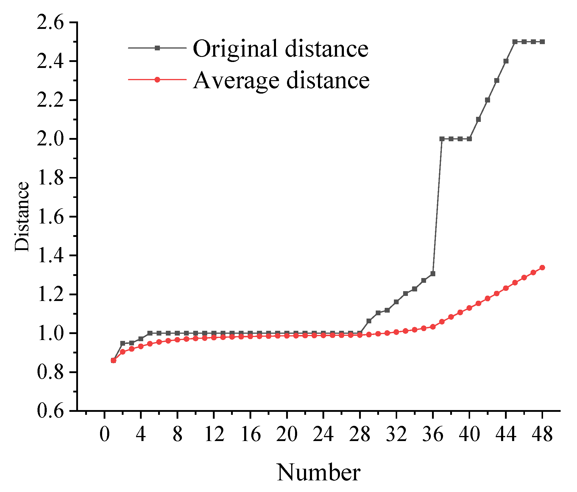
To evaluate the effects of various scales of noise on the point cloud, a sphere of radius R1 = 1 was simulated, with O as the center of sphere I; the 24 points on the surface of sphere I are normal points in the point cloud. The distribution of the distances from the 12 points to the center of the sphere O follows a Gaussian distribution, with mean and standard deviation . Specifically, the distances from the 12 points to O are {0.86, 0.948, 0.95, 0.971, 1.063, 1.105, 1.118, 1.161, 1.204, 1.228, 1.271, 1.306}, all of which constitute small-scale noise (Gaussian noise). The 12 points, distributed around the surface of sphere II (radius R2 = 2), represent large-scale noise points (anomalous noise) in the point cloud, and their distances from O are {2, 2, 2, 2, 2, 2.1, 2.2, 2.3, 2.4, 2.5, 2.5, 2.5, 2.5, 2.5}.
All of the points in the
k-neighborhood (
k = 2) were removed in the order of their original distance from the center (from small to large). For example, the distance to the first point is 0.86, with the average distance
, the distance of the second point is 0.948, with the corresponding average distance
, etc.; this allows a calculation of the average distance of the 48 points in the
k-neighborhood. The trend of the average distance and the original distance in the
k-neighborhood as a function of the number of points is shown in
Figure 1. For large-scale isolated points (anomalous noise), the average distance increased rapidly, and the distance from large-scale noise (
R2 = 2) to the center
O was relatively farther than the distance of normal points. Additionally, the average distance of the
k-nearest neighbors containing large-scale noise was greater than the average distance of
k-nearest neighbors not containing large-scale noise. These results indicated that anomalous noise can be filtered out directly via proper spatial distance. Therefore, we use distance-based feature information to separate the large-scale noise in this paper. Small-scale noise points are generally distributed in the vicinity of 1 and have less of an influence on the average distance; therefore, it is difficult to separate small-scale noise from the point cloud cluster by spatial distance. Instead, it is generally smoothed, according to the distribution law of Gaussian noise, to reduce the impact of small-scale noise on the follow-up. Therefore, we smooth small-scale noise based on vector information and noise distribution model in this paper.
2.2. Study Data and Evaluation Methods
2.2.1. Study Data
In order to test the performance of the algorithm proposed in the paper, six point cloud models from public datasets were selected as the research data, as shown in
Figure 2. The number of points for the Engine model was 3028, the number of points for the Blade model was 50,653, the number of points for the Building model was 93,039, the number of points for the Airplane model was 8176, the number of points for the Fish model was 3164, the number of points for the Cube model was 3177, the number of points for the People model was 5573, and the number of points for the Car model was 29,452. Large-scale noise, with a ratio of 0.02, and small-scale noise, of 20 dB, were added to the point cloud, where the small-scale noise represents Gaussian white noise.
Figure 2a shows the original point cloud,
Figure 2b shows the point cloud after adding large-scale noise,
Figure 2c shows the point cloud after adding small-scale noise, and
Figure 2d shows the point cloud after adding multi-scale noise. The experiments verifying the proposed algorithm were carried out based on these point cloud models.
2.2.2. Performance Evaluation
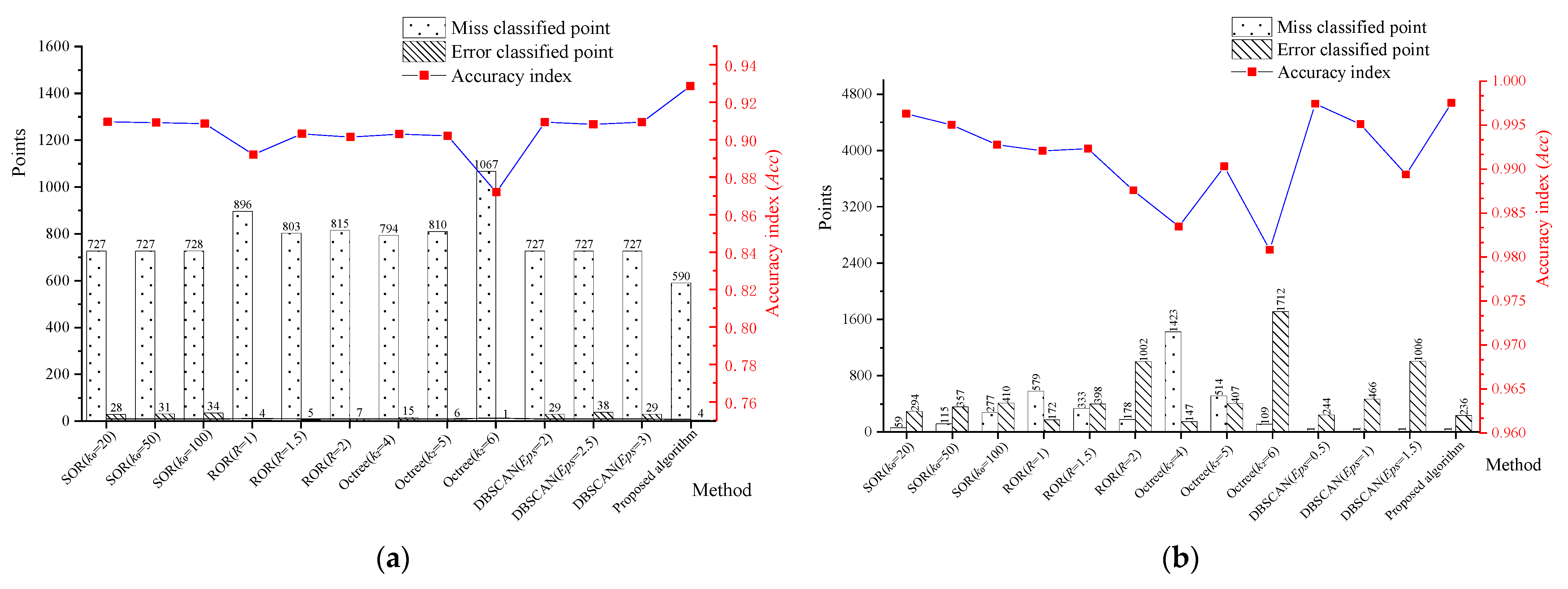
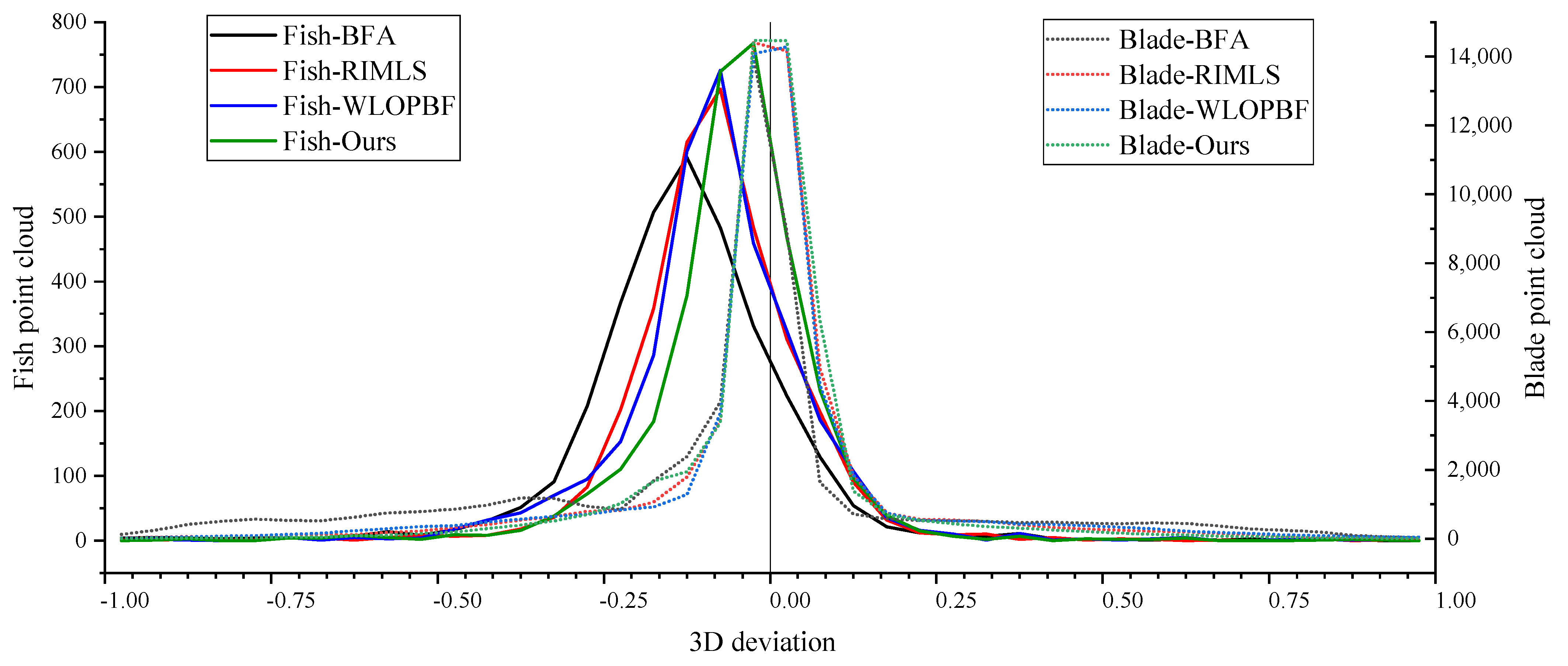
Since most current multi-scale filtering algorithms involve two-stage filtering methods (i.e., large-scale noise is filtered first, followed by small-scale noise), this paper compares the developed method with state-of-art large- and small-scale noise filtering algorithms to verify the large-scale noise denoising and small-scale noise photosmoothing abilities of the algorithm proposed in this paper.
A 3D comparison method was used to evaluate the noise filtering accuracy in this paper. Point clouds, filtered by various methods, were compared with the original noise-free point clouds in three dimensions, and the deviation distribution was obtained; the deviation values were counted to evaluate the advantage of the filtering algorithm in terms of filtering accuracy. However, isolated points are removed during 3D reconstruction, which affects the assessment of large-scale noise filtering effects; therefore, it is necessary to increase the objective evaluation index of large-scale noise filtering efficiency. The accuracy index (
Acc) was used in this work to assess the large-scale noise filtering effect; the accuracy index represents the ratio of the total number
Tu of all correctly classified points (correctly detected large-scale noise and normal points) to the total number of all elements in the classification task, as presented in Equation (1), where
Fa denotes the total number of miss classified points and error classified points. The miss classified points were generally large-scale noise points that were incorrectly classified as normal points, and the error classified points were normal points that were incorrectly classified as large-scale noise points.
Let us define the attribute information
Pi of the
k-nearest neighbor centroid as presented in Equation (2). Then
Pi indicates the dispersion contribution of the point to the neighborhood, such that the smaller the value of
pi, the richer the detail of the point cloud.
Entropy in information theory describes the uncertainty in the appearance of certain data, such that a higher entropy value indicates less information. Grey relation entropy theory is generated by combining grey relation analysis with entropy theory. Let a discrete sequence
X = {
Pi|
i = 1,2,…,
n}, containing
n elements and
, be defined, such that
,
is the grey entropy of the sequence
X, as presented in Equation (3) [
24,
25]. The total grey entropy of the point cloud indicates the amount of the detailed feature information contained in the point cloud. The smaller the value of
, the more chaotic the point cloud, more information it contains, and more it contributes to the geometric features of the region; this also means information contained is richer and more detailed. Additionally, when all values in the sequence are equal, the maximum grey entropy value of the sequence
X is ln
n, so the less high frequency information, the higher the grey entropy value.
The average grey entropy (AGE) of the point cloud represents the average geometric feature contribution of each point in the point cloud, and this parameter
ph is defined as presented in Equation (4) [
25]:
2.3. Methodology
Because conventional point cloud noise filtering algorithms have difficulty achieving single-stage adaptive filtering of multi-scale noise, an adaptive single-stage, multi-scale noise filtering algorithm for point clouds, based on feature information, is proposed herein. Scattered point clouds do not have a clear topology. Therefore, an efficient kd-tree topological data structure with multidimensional data indexing was adopted in this study. The distanced from each point within the
k-nearest neighborhood to the center point and the normal vector of each point in the
k-neighborhood based on the kd-tree were obtained. The normal vector was corrected via Gaussian filtering and a kd-tree traversal method, and the average normal vector angle
θ in the
k-neighborhood was obtained. The adaptive threshold-based point cloud segmentation algorithm divided the point clouds into large-scale noise (
LSN), feature-rich regions (
FRR), and flat regions (
FR) and processed them by removing noise, as well as applying the improved bilateral filtering algorithm and weighted mean algorithm based on grey relation analysis (WMGRA), respectively. This method effectively enabled rapid, single-stage, multi-scale noise filtering of noisy point clouds. The flow chart of the proposed algorithm is shown in
Figure 3.
All points (n) in the point cloud comprise of the point cloud scatter coefficient sequence and point cloud similarity degree sequence .
By determining the appropriate separation threshold
thd of
D and separation threshold
thθ of
Θ, through the adaptive threshold acquisition method (
Section 2.3.3), the discriminant function of each region segmentation could be obtained using Equation (5).
For large-scale noise, the noise-removal process was performed directly. Small-scale noise was mainly Gaussian noise, which was effectively processed via WMGRA denoising, which embodies the advantages of low algorithm complexity and short computational durations. However, it destroys the point cloud details in feature-rich regions, resulting in the blurring of edge and corner points of the cloud. Therefore, to remove the noise, while maintaining the high-frequency features of the target, the proposed method employed WMGRA (
Section 2.3.4) for small-scale noise smoothing in flat regions and an improved bilateral filtering algorithm (
Section 2.3.5) for small-scale noise smoothing in feature-rich regions.
2.3.1. Normal Vector Estimation and Correction
The point clouds (shown in
Figure 2) are a typical scattered point cloud without a clear topology, so we used a dichotomous tree (kd-tree) data structure to construct the basic topology of these point clouds in this paper, and the normal vectors were estimated using principal component analysis (PCA) in the k-neighborhood [
26,
27,
28].
Assuming that the set of points in the
k-neighborhood
X = {
qi |i = 1,2,k} and
k is the number of point clouds in the neighborhood, the covariance matrix of
X is defined as presented in Equation (6):
where
C represents the extent to which points in the
k-neighborhood deviate from the center of mass
. In this case,
C has three non-negative real eigenvalues, and the normal vector
of the feature point is the eigenvector corresponding to the smallest eigenvalue. Although
represents the direction of least change for all points in the neighborhood and has some noise immunity, the normal vector in the neighborhood will have discontinuous directions when the point cloud is cluttered; therefore, the estimated normal vector must be corrected.
All points were traversed according to the kd-tree topology, and the normal vector orientations of all points were corrected to be consistent. According to the vector dot product, when the normal vector
of the central feature point and the normal vectors of other points in the
k-neighborhood are negative, i.e., indicating two vectors have opposite directions, the direction of the seed point is favored, as presented in Equation (7).
To ensure that the normal vector in the
k-neighborhood varies continuously, the weighted mean filter was used in this study, and the normal vector correction model is given in Equation (8):
where
is the normal vector of points in the
k-neighborhood,
represents the Euclidean distance between points
and
, and
represents the influence factor of the Euclidean distance to
in the
k-neighbourhood on
. The radius of the
k-neighbourhood is taken in this paper.
2.3.2. Point Cloud Scatter Coefficient and Similarity Degree
The mean distance of the
k-nearest neighbors containing large-scale noise is greater than the mean distance of
k-nearest neighbors not containing large-scale noise; thus, we define the point cloud scatter coefficient (
PSC) within the
k-nearest neighbors based on this feature. Specifically,
PSC represents the point cloud dispersion within the
k-nearest neighbors. The larger the
PSC, the more discrete and sparser the point cloud distribution, and the higher the probability that the
k-nearest neighbors contain large-scale noise. The
PSC is defined as presented in Equation (9).
The point cloud similarity degree (
PSD) describes the directional consistency of the normal vectors of the points and centroids in the
k-nearest neighborhood. The larger the
PSD, the closer the normal vector directions of the points, and the
PSD is determined as presented in Equation (10).
2.3.3. Adaptive Threshold Acquisition Algorithm
The normal vector directions of the points in the flat region were generally consistent, whereas the normal vector directions of the points in the feature-rich region (including high-frequency feature information and small-scale noise) were more diverse. According to this parameter, the target point cloud can be partitioned into a flat region and a feature-rich region by choosing a suitable threshold. For the processor to automatically perform the denoising filtration, the filtering algorithm must automatically determine the optimal threshold (th), according to the point clouds in an adaptive manner.
The sequence of point cloud eigenvalues is . Let Tt = th and t be the index of the corresponding serial number of Tt. Then, t can divide the sequence T into two parts, i.e., the background and target. When 1 < i ≤ t, the elements are background; when t < i ≤ n, the elements are target. Calculating the proportion of each element as , the total proportion of background elements is , and the total proportion of target elements is .
The mean of the background elements is
, the mean of the target elements is
, and the mean of the entire sequence is
[
29]. The separation evaluation criteria objective function is defined as presented in Equation (11).
If we let b1 < bG < b2, the larger the , the further the target element is from the interval where the background element is located, i.e., the better the value of the objective function of the evaluation criterion, the more effective the separation. All separation evaluation criterion objective function values form the set , such that there must be a maximum criterion objective function value. In other words, there is an optimal separation point k*, such that , and the best separation is achieved when a threshold is selected.
2.3.4. Weighted Mean Algorithm Based on Grey Relation Analysis
In 1982, Professor Deng founded the discipline of grey system theory for analyzing uncertain systems with the characteristics of “small data (sample size is small)” and “poor information (less useful information in the data)”. After more than 30 years of vigorous development, grey system theory has been applied to forecasting, planning, decision-making, gemology, clustering, control, etc. [
30,
31,
32,
33]. The distribution that small-scale noise obeys in the neighborhood is unknown, and the relationship between points in the neighborhood is also unknown, so the local information of points in the neighborhood to be processed is an uncertain system. Therefore, grey system theory is well applicable to point cloud noise filtering tasks. To this end, we make the first attempt to apply grey system theory to point cloud noise processing in this paper. Grey relation analysis (GRA) is an important branch of the grey theory system. It can be used to measure the similarity and proximity between two grey systems. Small-scale noise points are far from the median of the neighborhood in the flat regions, so the similarity and proximity between systems
CA (consists of small-scale noise points) and
CB (Consists of the mean of the k-neighborhood) is very low. According to this feature, we propose a small-scale noise filtering algorithm for flat regions, based on WMGRA, in this paper.
In the k-neighborhood, the angle of the normal vector is related to the grey comparison sequence used for grey relation analysis.
The mean of the k-neighborhood is an element of GRA, and the grey reference sequence is . Small-scale noise obeys a Gaussian distribution, so the weighted mean value algorithm based on GRA (WMGRA) can smooth the small-scale noise in flat regions.
The grey reference sequence is subjected to a dimensionless unitary transformation of the initial values with the comparison sequence (Equation (12)).
The proximity of each element in the grey comparison sequence to the corresponding element in the reference sequence is computed using Equation (13).
The small-scale noise filtering factor
β in the flat region is defined as presented in Equation (14).
In this paper, the degree of proximity
r(
j) serves as the weight assignment coefficient, and the points after filtering the flat region are obtained using Equation (15); the time complexity of the WMGRA is
O(n):
where
is the filtered point,
is the original point,
is the normal vector at
, and
β is the mall-scale noise filtering factor defined by Equation (14). The small-scale noise filtering task is completed by moving the processing point
a certain distance along the direction of the normal vector
.
2.3.5. Improved Bilateral Filtering Algorithm
The point cloud bilateral filtering algorithm is based on development of image bilateral filtering, which accounts for the spatial Euclidean distance between pixel points in the k-neighborhood and the differences in the normal vectors of each point. This process can be described as a point moving a certain distance in its normal direction. Therefore, the bilateral filtering algorithm is generally used as a smoothing process for small-scale noise, and it cannot effectively remove anomalous noise points. The bilateral filtering algorithm based on point cloud data is presented in Equation (16) [
14,
34]:
where
is the filtered point,
is the original point,
is the normal vector at
, and
α is the bilateral filtering factor defined by Equation (17):
where
Rk is a set of the nearest neighbors of the central point
,
is a point within
Rk,
is the normal at the point
,
is the normal at the point
,
is the Euclidean distance between points
and
,
denotes the length of the projection of
in the direction of
normal to
,
is the Gaussian kernel function, and
is the Euclidean distance from
to
in the
k-neighborhood for
. The larger the
, the better the effect on the smoothness of the point cloud and larger the average distance from all points in the
k-neighborhood to
. The expression
is another form of the Gaussian kernel function, where
is the effect of the projection distance of each point in the
k-neighborhood on the normal vector of
on
; the larger the effect, the better the retention of the feature. The value of
σr is generally the standard deviation of the set of projected distances of the points on the
normal vector [
15].
Because the WMGRA ignores the distance information between points, the high-frequency feature points will be over-smoothed when using this method to process the feature-rich region. Typically, a bilateral filtering algorithm is used to smooth the feature-rich region of the point cloud. However, the traditional bilateral filtering factor uses the projection distance of neighboring points on their tangent planes as the weighting factor, which has some limitations in the sharp region, where the feature changes are more drastic.
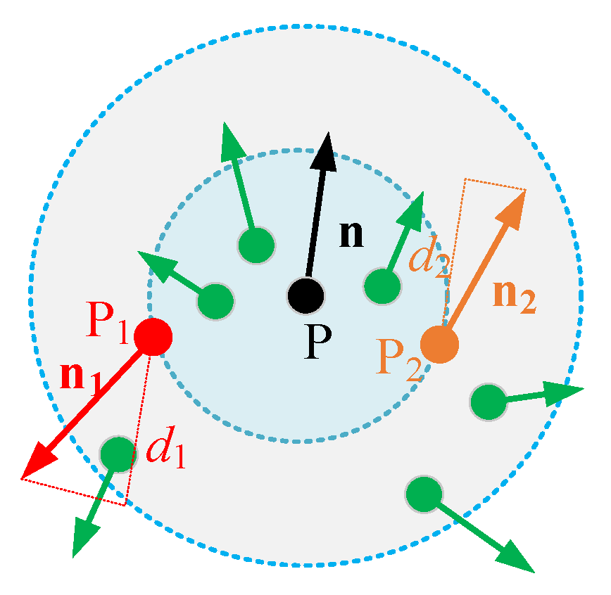
For the feature-rich region of the point cloud shown in
Figure 4, it is necessary to maintain the high-frequency feature of point
P. The projection lengths of
and
on
are the same, i.e.,
d1 = d2, if the traditional bilateral filtering factor is used. Accordingly, the impacts of
and
on
are the same, but the weight of
should be larger than that of
to maintain the feature of
P.
The cosine of the angle between the normal vectors was used as the feature retention factor of the bilateral filtering factor; thus, the weight was minimized when the angle is 90°. When the normal vector of each point in the k-neighborhood is relatively consistent with the direction of the normal vector of the point to be sought, there is a smaller angle between the two vectors, and the corresponding assigned weight should be larger. The definition of the improved bilateral filtering factor α is presented in Equation (18), where
, and
denotes the Euclidean distance between
and
.
The filtered points of the feature-rich region were obtained using Equation (19), and the time complexity of the improved bilateral filtering algorithm is
O(n
2).
4. Discussion
The accuracy of normal directly affects the filtering effect of noise. Therefore, one of the important future directions of noise filtering algorithm is the normal vector filtering algorithm. Sun et al. proposed a normal vector filtering method based on weighted averaging of neighboring normal [
16]. However, it uses a constant angle threshold, which makes it difficult to achieve the best filtering effect. To this end, Liang et al. proposed an adaptive angle threshold acquisition method, which achieved a better normal vector filtering and point cloud smoothing effect, but the complexity of the algorithm is high, and the parameters in the threshold acquisition model are difficult to determine [
36]. In order to deal with these problems, we propose a vector estimation and correction algorithm, based on directional discrimination and Gaussian filtering; the results show that the point cloud normal vector estimated by this method is more regular and smoother, compared to the traditional MLS method.
None of these conventional approaches to date achieves single-stage, multi-noise filtering, these methods typically use a serial (two-stage) processing model to achieve the tasks [
9,
21,
22]. In general, large-scale noise is usually sensitive to the distance in the neighborhood, while small-scale noise is usually related to the angle between the normal vectors in the neighborhood. To this end, we obtain the feature information of each point by traversing all points through an efficient kd-tree and achieve multi-scale noise filtering by partitioned parallel processing, based on feature information (point cloud scatter coefficient, PSC; point cloud similarity degree, PSD). Our results suggest that the algorithm proposed in this paper can single-stage quickly and adaptively (i) filter out large-scale noise, (ii) smooth small-scale noise, and (iii) effectively maintain the geometric features of the point cloud.
To objectively evaluate the comprehensive performance of the algorithms proposed in this paper, first, we compared the developed method with state-of-art large-scale filtering algorithms to verify the large-scale noise denoising abilities of the proposed method; then, we compared the developed method with state-of-art, small-scale noise filtering algorithms to verify the small-scale noise photosmoothing abilities of the proposed algorithm. Moreover, we propose several filtering effect evaluation indexes. For example, for large-scale noise filtering evaluation, there are miss classified points index, error classified points index, and large-scale noise recognition accuracy rate index (Acc); for small-scale noise filtering evaluation, there are total grey entropy and average grey entropy (AGE). These indexes offer new ways to objectively evaluate the performance of the point cloud filtering algorithms.
There are two general ways to reduce the time for small-scale noise filtering, one of which is to design low-complexity algorithms [
16,
37], and the other is to partition the point cloud [
20]. In this paper, we use both of the above methods to reduce running time. First, a point cloud partitioning process is used to divide the point cloud into large-scale noise, a feature-rich region, and a flat region; these three regions can be handled separately later to reduce the waste of computing power. Second, a WMGRA-based, small-scale noise filtering algorithm for the flat region is designed in this paper, and the complexity of the algorithm is only
O(
n), so smooth tasks can be done quickly. Our results suggest that the running time of the proposed algorithm is minimal, compared to other state-of-the-art algorithms. Furthermore, we apply grey model theory to the field of point cloud filtering for the first time; these studies, thus, offer a new strategy to point cloud processing.
Although the proposed algorithm achieves single-stage, adaptive, multi-scale point cloud noise filtering, there are also limitations. First, the results show that the processing time of the algorithm is still too long to be applied to high-speed online processing platforms. For example, the complexity of the adaptive threshold acquisition method designed in this work is high, which needs to be improved in the future. Second, the normal vector, PSD, and PSC are related to the neighborhood size. Generally, the larger the neighborhood is, the more realistic and accurate the description of the point cloud is; therefore, the better the filtering effect is, but at the cost of increased computing time. The selection of neighborhood size in this paper is obtained empirically, and the effect of point cloud neighborhood on the filtering results is not investigated; so, how to select the neighborhood size appropriately is a future research direction. In addition, the set of feature information obtained in this paper is inconsistent, such as PSD is k-nearest neighbors and PSC is k-neighborhood; in addition, the adaptive threshold acquisition algorithm is based on the global. So, the set of all feature information needs to be unified in future study, but since different point cloud models (or different noise distribution, different noise content, etc.) correspond to different optimal choices, and the threshold selection method based on local information is sensitive to noise. Therefore, it is a very challenging task to unify all sets.
5. Conclusions
This paper proposes a fast, single-stage, adaptive, multi-scale noise filtering algorithm for point clouds. Based on the feature information (e.g., point cloud scatter coefficient and point cloud similarity degree), obtained by a kd-tree and the amended normal vector, the noise-containing point cloud is divided into three parts: large-scale noise, feature-rich regions, and flat regions. The large-scale noise is removed directly, and the feature-rich and flat regions are filtered using an improved bilateral filtering algorithm and WMGRA, respectively. The results confirm that the proposed algorithm can quickly and adaptively filter out large-scale noise and smooth, small-scale noise, while also effectively maintaining the geometric features of the point cloud.
In follow-up work, we will focus on the three aspects: optimizing the efficiency of the algorithm to improve filtering performance, reducing the complexity of the algorithm for adapting to high-speed online processing situations, and building more robust features information to improve point cloud region segmentation abilities.


 ,
, 


