An Analytic Solution to Precipitation Attenuation Expression with Spaceborne Synthetic Aperture Radar Based on Volterra Integral Equation

Abstract

Precipitation is closely related to the production and daily life of human beings, so accurate precipitation measurement is of great significance. Spaceborne synthetic aperture radar (SAR) is a microwave remote sensing technology with high resolution, which provides an opportunity to improve the accuracy of precipitation inversion. In this paper, the radar attenuation expression is analyzed according to the scattering characteristics of rain, snow and ground. Combined with the Volterra integral equation of the second kind, the solution to the expression, the precipitation horizontal variation of the double-layer model, can be obtained. The simulated result of this method is in good agreement with the given horizontal variation of precipitation. Compared with the original VIE method, which only considers the effect of rainfall, the method in this paper considers both rainfall and snowfall; compared with the Model Oriented Statistical (MOS) method, the method in this paper not only reduces the number of empirical coefficients used and thus reduces the workload in the early stage and retrieval process and its application limits, but it will also increase the accuracy of the inversion of the horizontal variation.

1. Introduction

Precipitation is a phenomenon that the water vapor in the atmosphere condenses and falls to the ground in the form of liquid water or solid water. It includes rain, snow, sleet, frost, hail, ice particles, etc. Human production and activities correlate with precipitation; thus, the accurate measurement of precipitation is particularly necessary [1,2]. At present, however, only a small number of countries can obtain relatively accurate distribution information of the global precipitation. Therefore, an increasing number of studies need to be carried out on global precipitation measurement.

Remote sensing is a comprehensive earth observation technology developed in the 1960s. Remote sensing technology has made great progress, and its application has been gradually more extensive since the 1980s. According to the principle that the ability to absorb and reflect electromagnetic waves differ from object to object, once such abilities of an object on the surface are detected, information can be extracted to identify the object from a long distance away, which offers potential to precipitation observations.

Synthetic aperture radar (SAR) is an all-weather, all-time high-resolution microwave imaging radar. It applies a synthetic aperture principle, pulse compression technology and a signal processing method, aiming at obtaining azimuth high-resolution and range high-resolution imaging with a real aperture antenna under a wide frequency range and different polarizations. The SAR system, providing useful information to human beings, has been extensively used in military, economic, scientific and technological fields, and has broader application prospects and greater development potential [3].

The frequency of radio waves working at X band is only 4 GHz lower than that working at Ku band, the working frequency band of precipitation radar (PR). Furthermore, studies have shown that X-SARs are more sensitive to precipitation than SARs operating under lower frequencies [4,5]. Many countries have successfully launched SAR systems carrying high-frequency X-band synthetic aperture radar (X-SAR) sensors, such as SRTM launched by America in 2000, Cosmo-Skymed launched by Italy in 2006, TerraSAR-X launched by German in 2007, etc. The benefits of using X-SAR to retrieve precipitation are as follows. First, the scale of the spaceborne radar antennas is limited, leading to a serious non-uniform beam filling effect and bringing great deviation to precipitation inversion [6]. Fortunately, this problem can be solved with a high-resolution X-SAR and microwave radiation measurement data. Second, precipitation measurement in mountainous areas is also an important topic. The terrain of such areas brings challenges to PRs while X-SARs provides a method for precipitation measurement in mountainous areas. Third, X-SARs can observe mid-latitude storms which Tropical Rainfall Measuring Mission (TRMM) might miss [7]. Thus, the observation results of X-SARs will supplement and enhance those of Global Precipitation Mission (GPM). Fourth, X-SARs used in the precipitation retrieval increases practical use of X-SAR satellite images and can improve the investment benefits of X-SARs.

Pichugin et al. established a single-layer, the rainfall layer, model for radar observation in 1991 [8]. They obtained the analytical solution to the horizontal rainfall variation of a single-layer model by solving the rainfall attenuation expression combining the Volterra integral equation (VIE) of the second kind. However, because the attenuation coefficients of different condensates (such as rain and snow) are different, this method cannot be directly applied to the model containing two or more condensates. Marzano et al. proposed a Model Oriented Statistical (MOS) method. They considered a more complex double-layer precipitation model with a snowfall layer and a rainfall layer completely separated in 2008 [9,10]. They analyzed the characteristics of radar backscattering cross section and obtained the statistical solution to the horizontal precipitation variation of a double-layer rainfall model. However, this method relies on many empirical values, thus having a large workload in the early stage. What makes the result less accurate is that it makes an approximation in retrieval of the shape of the precipitation area. Xie et al. proposed a MOSVI method, combining the MOS method and the VIE method [11]. They apply the VIE method to obtain information on the shape of the precipitation area and the MOS method to calculate the rain rate. It partially reduces the numbers of the empirical values of MOS method. To further reduce the numbers of the empirical values so as to reduce the workload in the early stage, an analytical method to obtain the horizontal variation of the double-layer precipitation model is proposed in this paper.

2. Principles and Model Establishment

The radar antenna only receives the energy that returns to the radar, which is called the backscattering energy. The total scattering power of a scattering particle is obtained by multiplying the incident wave energy flow density by the radar cross section (RCS). When the scattering particle makes isotropic scattering with this total power, the power density scattered to the antenna is just equal to the actual backscattering energy flow density caused by the particle at the antenna [12]. Thus, we can obtain the backscattering energy of the particle from its normalized radar cross section (NRCS) which can be divided into the surface backscattering cross section and the precipitation backscattering cross section:

$${\sigma }_{SAR}={\sigma }_{srf}+{\sigma }_{vol},$$

(1)

where ${\sigma }_{SAR}$ is the radar backscattering cross section, ${\sigma }_{srf}$ is the surface backscattering cross section, ${\sigma }_{vol}$ is the volume backscattering cross section.

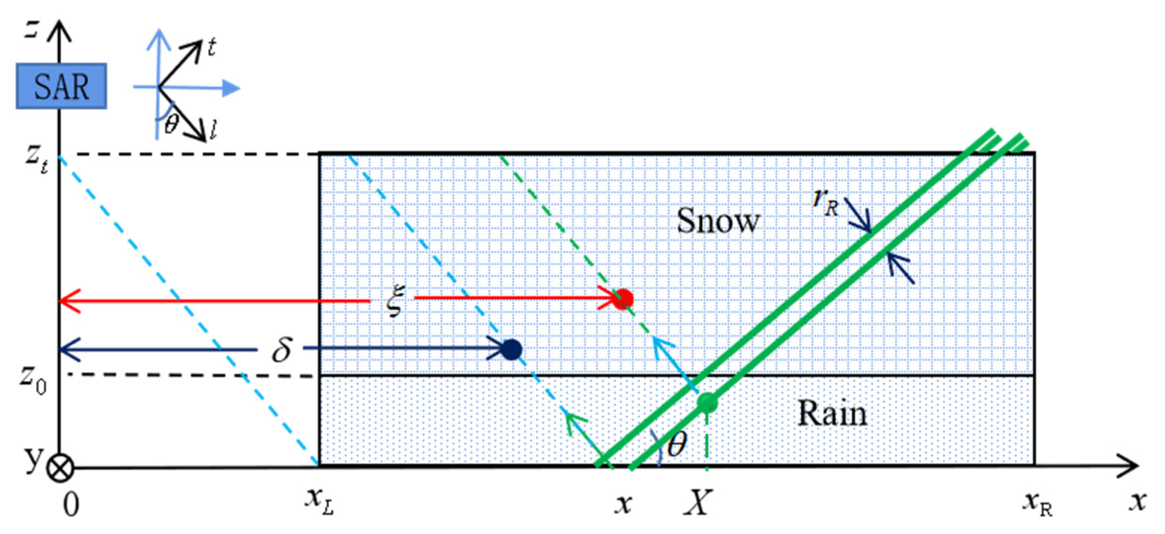
2.1. The Precipitation Cross Sectional Model

To simplify the precipitation model and reduce the method complexity, a lot of assumptions are made as follows. The microwave pulses emitted by the radar are treated as plane waves. Among all the hydrometeors, only the rainfall and snowfall are considered and seen as independent, which means the melting layer is ignored. The ground is considered as a plane terrain. The simplified cross sectional model of rainfall and snowfall is shown in Figure 1.

2.2. The Precipitation Spatial Distribution

The precipitation spatial precipitation rate is simplified as the factorization of the vertical distribution variation and its horizontal variation [9]:

$$R\left(x,z\right)=I\left(x\right)·V\left(z\right),$$

(2)

where $R\left(x,z\right)$ is the precipitation rate in $\mathrm{mm}/\mathrm{h}$, $V\left(z\right)$ is the vertical distribution of the precipitation and $I\left(x\right)$ is the horizontal variation of $V\left(z\right)$. The along-track resolution $·y$ is estimated to be 264$\mathrm{m}$ [10]. This degraded along-track resolution is adequate for hydrological purposes. This paper will focus on the solution to the horizontal variation $I\left(x\right)$. Thus, the vertical distribution $V\left(z\right)$ will be considered uniform for simplicity:

$$V\left(z\right)=V\left(0\right), 0\le z\le z_t,$$

(3)

where $V\left(0\right)$ is the near-surface precipitation rate in $\mathrm{mm}/\mathrm{h}$. $I\left(x\right)$ representing a single rain-cloud cell can be expressed as:

$$I\left(x\right)=\{\begin{array}{cc}\hfill 0,& 0\le x<z_t/\tan \theta \hfill \\ \hfill x/d-z_t/(\mathrm{dtan}\theta ),& z_t/\tan \theta \le x<d+z_t/\tan \theta \hfill \\ \hfill 1,& d+z_t/\tan \theta \le x<w-d+z_t/\tan \theta \hfill \\ \hfill \left(w-x\right)/d+z_t/(\mathrm{dtan}\theta ),& w-d+z_t/\tan \theta \le x<w+z_t/\tan \theta \hfill \\ \hfill 0,& x\ge w+z_t/\tan \theta \hfill \end{array}$$

(4)

where $d$ is the shape parameter of the horizontal variation of the precipitation, $w$ is the width of the precipitation area in km.

In this paper, three common cases for the horizontal variation with a single rain-cloud cell are used. For $d=0$:

$$I\left(x\right)=\{\begin{array}{cc}\hfill 0,& 0\le x<z_t/\tan \theta \hfill \\ \hfill 1,& z_t/\tan \theta \le x<w+z_t/\tan \theta \hfill \\ \hfill 0,& x\ge w+z_t/\tan \theta \hfill \end{array},$$

(5)

representing the rectangular variation.

For $d=w/2$:

$$I\left(x\right)=\{\begin{array}{cc}\hfill 0,& 0\le x<z_t/\tan \theta \hfill \\ \hfill \left(x-z_{t}tan\theta \right)/\left(w/2\right),& z_t/\tan \theta \le x<w/2+z_t/\tan \theta \hfill \\ \hfill \left(w-x+z_{t}tan\theta \right)/\left(w/2\right),& w/2+z_t/\tan \theta \le x<w+z_t/\tan \theta \hfill \\ \hfill 0,& x\ge w+z_t/\tan \theta \hfill \end{array},$$

(6)

representing the triangular variation.

For $0<d<w/2$, $I\left(x\right)$ represents the trapezoidal variation.

To specify, $I\left(x\right)$ representing two or more rain-cloud cells can be realized by superimposing two or more single rain-cloud cells accordingly. In this paper, the rectangular variation with two separate rain-cloud cells is also considered in the simulation and it can be expressed as:

$$I\left(x\right)=\{\begin{array}{l}0, 0\le x<z_t/\tan \theta \\ 1, z_t/\tan \theta \le x<d+z_t/\tan \theta \\ 0, d+z_t/\tan \theta \le x<w-d+z_t/\tan \theta \\ 1, w-d+z_t/\tan \theta \le x<w+z_t/\tan \theta \\ 0, x\ge w+z_t/\tan \theta \end{array}.$$

(7)

2.3. Normalized Radar Cross Section Analysis

Assume that the average surface backscattering cross section of ground is ${\mathsf{\sigma }}_0$. When the radar beam enters the area with hydrometeors which are rain and snow in this paper, the surface scattering echoes will be attenuated:

$${\sigma }_{srf}\left(x\right)={\sigma }_0·L^2\left(x\right),$$

(8)

where $L$ is the one-way atmospheric loss factor, relevant to the path of the radar beam. Then, Equation (8) can be rewritten as:

$${\sigma }_{srf}\left(x\right)={\sigma }_0·exp(-2/\sin \theta {{\displaystyle \int }}_{x_{s_1}}^{x_{s_2}}k\left(\delta \right)d\delta ),$$

(9)

where $x_{s_1}$ and $x_{s_2}$ are the $x$-coordinates of the left and right limits of the attenuation path of the scattering echo along $l$-direction caused by ground.

Similarly, when the radar beam enters the area with hydrometeors, the precipitation scattering echoes will be attenuated:

$${\sigma }_{vol}\left(x\right)=\tan \theta {{\displaystyle \int }}_{x_{v_1}}^{x_{v_2}}{L}^2\left(x\right)·\eta \left(\mathrm{X}\right)\mathrm{dX},$$

(10)

where $x_{v_1}$ and $x_{v_2}$ are the $x$-coordinates of the left and right limits of the attenuation path of reflecting along $t$-direction caused by meteorological particles. Furthermore, it can also be rewritten as:

$${\sigma }_{vol}\left(x\right)=\tan \theta {{\displaystyle \int }}_{x_{v_1}}^{x_{v_2}}exp\left(-2/\sin \theta {{\displaystyle \int }}_{x_{v_3}}^{x_{v_4}}k\left(\xi \right)d\xi \right)\eta \left(X\right)dX,$$

(11)

where $x_{v_3}$ and $x_{v_4}$ are the $x$-coordinates of the left and right limits of the attenuation path of scattering echo along $l$-direction caused by meteorological particles. $\eta$ is the radar reflectivity, defined as the summation of radar cross sections of all precipitation particles per unit volume, relevant to the distribution and size of the meteorological particles and the frequency of the microwaves. A widely accepted way to express $\eta$ [13,14] is that:

$$\mathsf{\eta }\left(x\right)=\frac{{\pi }^5{\left|K_0\right|}^2}{{\lambda }^4}{i}_1{\left[R\left(x\right)\right]}^{b_1}=a_1{\left[R\left(x\right)\right]}^{b_1},$$

(12)

where ${\left|K_0\right|}^2$ is an expression of negative refractive index, which is approximately 0.19 for snow and 0.93 for rain when neglecting the influence of the temperature. Furthermore, $\lambda$ is the wavelength of electromagnetic waves, which is about 3.1 $\mathrm{cm}$ for X-band SAR. $i_1$ and $b_1$ are empirical values. Lots of studies have been carried out on the values of $i_1$ and $b_1$. In this paper, the values calculated by Ulaby [15] (pp. 318–328) are adopted. For rain, $i_1$ is 300, $b_1$ is 1.1; for snow, $i_1$ is 182, $b_1$ is 1.4.

2.4. Extinction Coefficient k

Scatterers (rain, snow and other hydrometeors) are generally considered to be randomly distributed, and assume that there is no coherent phase relationship between the scattering fields of each single particle. Therefore, the volume absorption and scattering containing many particles can be calculated through incoherent scattering theory. According to the different attenuation effects of rainfall and snowfall, the attenuation coefficient $k$ will be expressed by $k_r$ and $k_s$ respectively. For a given droplet size distribution $p\left(r\right)$, where $r$ is the droplet size, the rainfall extinction coefficient can be calculated [15] (pp. 318–326):

$$k_r\left(x\right)=\frac{{\lambda }^3}{8{\pi }^2}{{\displaystyle \int }}_0^{\infty }{\chi }^{2}p\left(\chi \right){\varsigma }_e\left(\chi \right)\mathrm{d}\mathsf{\chi },$$

(13)

$$\chi =\frac{2\pi r}{\lambda },$$

(14)

where ${\varsigma }_e$ is the attenuation coefficient of Mie Scattering. Furthermore, the snowfall extinction coefficient can be calculated [15] (pp. 326–328):

$$k_s\left(x\right)=4.34\times {10}^{-4}\left[\frac{2\times {10}^{-3}{\pi }^5}{3{\lambda }^4{\rho }_s{}^2}{\left|K_{ds}\right|}^2{{\displaystyle \sum }}_{i=1}^{N_v}{d}_i{}^6+\frac{{\pi }^2}{\lambda {\rho }_s}Im\left\{-K_{ds}\right\}{{\displaystyle \sum }}_{i=1}^{N_v}{d}_i{}^3\right],$$

(15)

where ${\rho }_s$ is the density of snowfall, $K_{ds}$ is related to the refraction of dry snow, $d_i$ is diameter of snowfall, $N_v$ is the total number of droplets per unit volume.

Such theoretical method of calculating the extinction coefficient of rainfall and snowfall are widely proved effective and many scholars have calculated the values under a wide range of frequencies [16,17,18]. However, due to its complexity, this method is difficult to be directly applied to a certain algorithm. To simplify the acquisition of the extinction coefficients, Ryde [19] proposed a linear relationship between the extinction coefficients and the precipitation:

$$k\left(x\right)=a·R\left(x\right),$$

(16)

where $R$ is the precipitation in $\mathrm{mm}/\mathrm{h}$, $a$ is an empirical value. Later, a logarithmic relationship between the extinction coefficients and the precipitation is proposed and used [20,21,22]:

$$k\left(x\right)=a·R{\left(x\right)}^b,$$

(17)

where $a$ and $b$ are both empirical coefficients. Scholars have conducted extensive research on the empirical coefficients of Equations (16) and (17) [23,24,25,26,27,28]. Furthermore, their root mean square (rms) errors are listed in

Table 1. The root mean square(rms) error of the linear model in Equation (16) and the logarithmic model in (17) [15].

Frequency (GHz)	rms Error of (17) (Percent)	rms Error of (16) (Percent)
7.5	28	31
9.4	30	36
16.0	22	28
34.9	10	12

. It is obvious that the rms errors of the linear model are slightly larger than those of the logarithmic model. However, using the logarithmic model will largely increase the complexity of the method introduced in this paper and the rms error of the linear model is acceptable, so in this paper, the linear model is adopted. The values calculated by Ulaby [15,21] are adopted. For rain, $a=3.349\times {10}^{-3}$; for snow, $a=2.229\times {10}^{-3}$.

2.5. Analysis of Radar Backscattering Echo Path

Based on the cross sectional model established in Section 2.1, it is convenient to analyze the radar backscattering echo path, as is shown in Appendix A. Furthermore, explicit NRCS formulas under different precipitation ranges can be derived with the analysis of the paths of the radar backscattering echoes.

According to the analysis of the path of the radar echoes and the effect of precipitation on radar echoes, it is obvious that the paths of different radar echoes, the extinction coefficients and the radar reflectivity are different under different precipitation ranges. Thus, attention should be paid during the simulation.

3. Volterra Integral Equation (VIE) of the Second Kind Inversion Method

Since the extinction coefficient $k$ and the radar reflectivity $\eta$ will be zero, according to Equations (12) and (16), if the precipitation rate is zero, we can easily integrate the numerous formulas in Appendix A into one:

$$\begin{gathered} {\sigma }_{SAR}\left(x\right)={\sigma }_{0}exp\left[-\frac{2}{\sin \theta }\left({{\displaystyle \int }}_{x-z_t\tan \theta }^{x-z_0\tan \theta }{k}_s\left(\delta \right)d\delta +{{\displaystyle \int }}_{x-z_0\tan \theta }^x{k}_r\left(\delta \right)d\delta \right)\right]+ \\ \tan \theta {{\displaystyle \int }}_{x+z_0/\tan \theta }^{x+z_t/\tan \theta }exp\left(-\frac{2}{\sin \theta }{{\displaystyle \int }}_{X-\left[z_t-\left(X-x\right)\tan \theta \right]\tan \theta }^X{k}_s\left(\xi \right)d\xi \right){\eta }_s\left(X\right)dX+ \\ \tan \theta {{\displaystyle \int }}_x^{x+z_0/\tan \theta }exp\left[-\frac{2}{\sin \theta }\left({{\displaystyle \int }}_{X-\left[z_t-\left(X-x\right)\tan \theta \right]\tan \theta }^{X-\left[z_0-\left(X-x\right)\tan \theta \right]\tan \theta }{k}_s\left(\xi \right)d\xi +{{\displaystyle \int }}_{X-\left[z_0-\left(X-x\right)\tan \theta \right]\tan \theta }^X{k}_r\left(\xi \right)d\xi \right)\right]{\eta }_r\left(X\right)dX. \end{gathered}$$

(18)

This nonlinear formula, however, is not easy to deal with. To simplify this formula, we can introduce a function:

$$p\left(x\right)=exp\left(\frac{2}{\sin \theta }{{\displaystyle \int }}_0^x{k}_r\left(m\right)dm\right).$$

(19)

Using $p\left(x\right)$, the extinction coefficients of rain, the radar reflectivity of rain and snow, together with the precipitation rate can also be expressed, as is derived in Appendix B. After the substitution and transformation, also shown in Appendix B, we can obtain:

$$\begin{gathered} p{\left(x\right)}^{\frac{a_s}{a_r}}=f_1\left(x\right)-{\lambda }_1{{\displaystyle \int }}_{x+z_0/\tan \theta +z_0\tan \theta }^{x+z_t/\tan \theta +z_t\tan \theta }{K}_3\left(\mathrm{X}\right)p{\left(t\right)}^{\frac{a_s}{a_r}}dt \\ -{\lambda }_2{{\displaystyle \int }}_x^{x+z_0/\tan \theta +z_0\tan \theta }{K}_4\left(\mathrm{X}\right)p{\left(t\right)}^{\frac{a_s}{a_r}}dt, \end{gathered}$$

(20)

where

$$f_1\left(x\right)=\frac{{\sigma }_{SAR}\left(x+z_t\tan \theta \right)·p\left(x+z_t\tan \theta \right)·p{\left[x+\left(z_t-z_0\right)\tan \theta \right]}^{\frac{a_s}{a_r}-1}}{{\sigma }_0},$$

(21)

$$K_3\left(\mathrm{X}\right)=K_1\left(\mathrm{X}\right)·p{\left[x+\left(z_t-z_0\right)\tan \theta \right]}^{\frac{a_s}{a_r}-1}·p\left(x+z_t\tan \theta \right),$$

(22)

$$K_4\left(\mathrm{X}\right)=K_2\left(\mathrm{X}\right)·p{\left[x+\left(z_t-z_0\right)\tan \theta \right]}^{\frac{a_s}{a_r}-1}·p\left(x+z_t\tan \theta \right),$$

(23)

$${\lambda }_1=\frac{G_1{\cos }^2\theta }{{\sigma }_0},$$

(24)

$${\lambda }_2=\frac{G_2{\cos }^2\theta }{{\sigma }_0}.$$

(25)

Assume that for $x\ge x_m$, there is no precipitation; that is $I\left(x\right)=0$. According to Equations (16) and (19), for $I\left(x\right)=0$, we can always obtain $k\left(x\right)=0$ and $p\left(x\right)=1$. Then, we can obtain the values of $K_3\left(\mathrm{X}\right)$, $K_4\left(\mathrm{X}\right)$, $K_1\left(\mathrm{X}\right)$, $K_2\left(\mathrm{X}\right)$ and $f_1\left(x\right)$ for $x_m-\left(z_t-z_0\right)\tan \theta \le x\le x_m$. Furthermore, naturally, we can obtain $p\left(x\right)$ for $x_m-\left(z_t-z_0\right)\tan \theta \le x\le x_m$. Furthermore, we can then obtain $p\left(x\right)$ for $x_m-\left(n+1\right)\left(z_t-z_0\right)\tan \theta \le x\le x_m-n\left(z_t-z_0\right)\tan \theta$, where n is a non-zero natural number. Through such iterations, we can obtain $p\left(x\right)$ under ranges of interest. The iteration processes are explicitly shown in Appendix B.

4. Simulation Results

For X-band SAR working at the oblique angle of 30°, ${\sigma }_0$ is approximately −7 dB [29]. Set $z_t=13 \mathrm{km}$ and $z_0=4.5 \mathrm{km}$. From Equations (12), (16) and (18), we can first obtain the normalized radar cross section (NRCS) ${\sigma }_{SAR}$ of the double-layer precipitation model. With Formulas (6) or (7), we can obtain the horizontal precipitation variation of the model. Taking a rectangular rain-cloud cell, a trapezoidal rain-cloud cell, a triangular rain-cloud cell and two separate rectangular rain-cloud cells under the rain rate of 10$\mathrm{mm}/\mathrm{h}$ as Examples 1–4, the precipitation variation simulation result diagrams, given precipitation variation diagrams, comparison diagrams and absolute error diagrams are shown in Figure 2, Figure 3, Figure 4 and 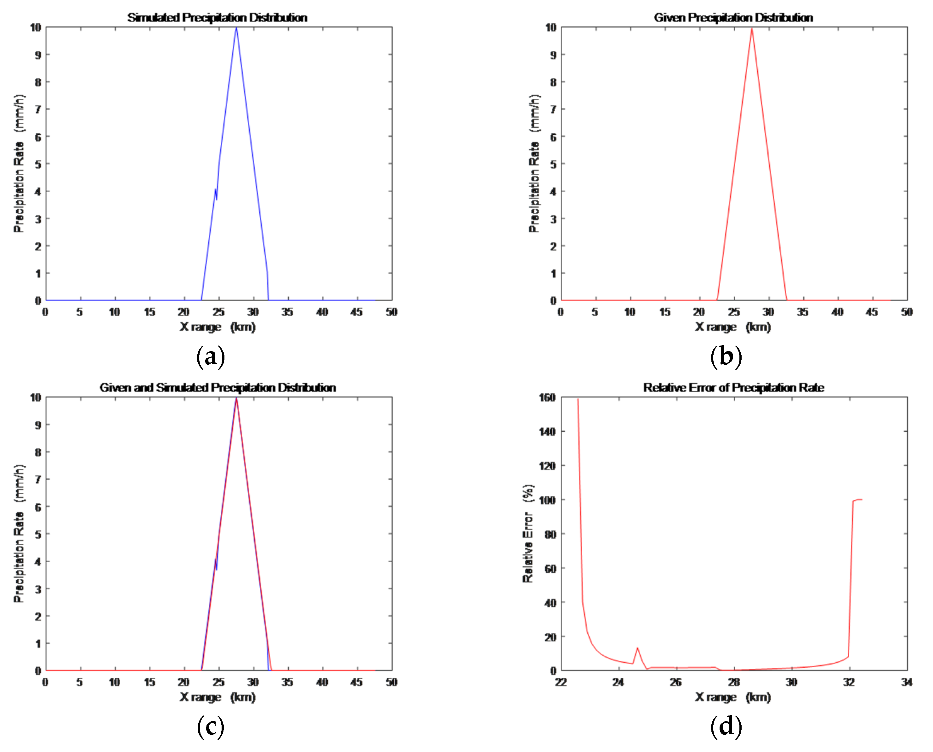Figure 5. Taking a triangular rain-cloud cell under the rain rate of 30$\mathrm{mm}/\mathrm{h}$ and 50$\mathrm{mm}/\mathrm{h}$ as Examples 5–6, the precipitation variation simulation result diagrams, given precipitation variation diagrams, comparison diagrams and relative error diagrams are shown in Figure 6 and Figure 7. The attributes of the six examples, including the maximum rain rate $R$($x$), the width of the rain-cloud cells $w$, the shape parameters $d$ and the shapes of rain-clouds are listed in

Table 2. The attributes of the 6 examples.

	$\mathbf{Maximum} \mathit{R}$$(\mathit{x}$$) (\mathbf{m}\mathbf{m}/\mathbf{h})$	$\mathit{d}$$\left(\mathbf{k}\mathbf{m}\right)$	$\mathit{w}$$\left(\mathbf{k}\mathbf{m}\right)$	Shape of Rain-Cloud(s)
1	10	0	10	Rectangular
2	10	3	10	Trapezoidal
3	10	5	10	Triangular
4	10	2.5	2.5	Rectangular bimodal
5	30	5	10	Triangular
6	50	5	10	Triangular

. The simulation results of the attributes are listed in

Table 3. Simulation result of the 6 examples.

	$\mathbf{Maximum} \widehat{\mathit{R}}$$(\mathit{x}$$) (\mathbf{m}\mathbf{m}/\mathbf{h})$	$\tilde{\mathit{R}}$$\left(\mathit{x}\right)$	$\widehat{{w}}$$\left(\mathbf{k}\mathbf{m}\right)$	$\tilde{\mathit{w}}$	Shape of Rain-Cloud(s)
1	10.07	0.7%	10.1731	1.731%	Rectangular
2	10.08	0.8%	9.8552	1.448%	Trapezoidal
3	9.965	0.35%	9.8552	1.448%	Triangular
4	10.09	0.9%	2.56	2.4%	Rectangular bimodal
5	29.9	1%	9.8552	1.448%	Triangular
6	49.83	1.7%	9.9255	0.745%	Triangular

, where $\widehat{R}$($x$) is the simulated result of the maximum rain rate, $\tilde{R}$($x$) is the relative error of the maximum rain rate, $\hat{\mathrm{w}}$ is the simulated result of the width of the rain cloud and $\tilde{w}$ is the relative error of the width of the rain cloud.

According to Figure 2, Figure 3, Figure 4, Figure 5, Figure 6 and Figure 7, it is obvious that large errors occur at the edges of the precipitation area. The relative errors of the rest areas of the simulation results will be listed for each example.

Example 1.

Due to the non-linearity, fluctuations occur at each junction, which is${\widehat{x}}_R-n·\left(z_t-z_0\right)\tan \theta$or${\widehat{x}}_R-n·z_t\tan \theta$, where n is a natural number. Except the right edge,$\widehat{R}\left(x\right)$is in the range of$\left[9.9,10.07\right] mm/h$in the precipitation area, and the maximum relative error is 1%.

Example 2.

The error 8.073% occurs at the junction,${\widehat{x}}_R-z_t\tan \theta$, due to the non-linearity. In the rest of the precipitation area, the relative error of$\widehat{R}\left(x\right)$is less than 3%.

Example 3.

The error at the junction,${\widehat{x}}_R-z_t\tan \theta$, is 13.47%. In the rest of the precipitation area, maximum relative error of$\widehat{R}\left(x\right)$is 1.7%.

Example 4.

Due to the non-linearity, fluctuations occur at each junction, which is${\widehat{x}}_R-n·\left(z_t-z_0\right)\tan \theta$or${\widehat{x}}_R-n·z_t\tan \theta$, where n is a natural number. Except the edges and the junctions,$\widehat{R}\left(x\right)$is in the range of$\left[10.07, 10.09\right] mm/h$in the precipitation area, maximum relative error is 0.9%.

Example 5.

The error at the junction,${\widehat{x}}_R-z_t\tan \theta$, is 12.41%. In the rest of the precipitation area, maximum relative error of$\widehat{R}\left(x\right)$is less than 2%.

Example 6.

The error of$\widehat{R}\left(x\right)$around the junction${\widehat{x}}_R-z_t\tan \theta$is 13.12%. In the rest of the precipitation area, maximum relative error of$\widehat{R}\left(x\right)$is 1.8%.

5. Discussion

In Section 4, Examples 1–4 are the simulations under the maximum rain rate of $10 \mathrm{mm}/\mathrm{h}$ with different shapes of the rain-cloud cells, that is the rectangular rain-cloud cell, the trapezoidal rain-cloud cell, the triangular rain-cloud cell and the rectangular bimodal rain-cloud cell. It is obvious that the simulated result using this method is in good agreement with the given distribution. Besides different shapes of the rain-cloud cells, this method can also be applied to different rain rates. Examples 1, 5 and 6 are the simulations under the maximum rain rates of $10 \mathrm{mm}/\mathrm{h}$, $30 \mathrm{mm}/\mathrm{h}$ and $50 \mathrm{mm}/\mathrm{h}$ with a triangular rain-cloud cell. The typical value $30 \mathrm{mm}/\mathrm{h}$ is chosen because the melting layer, the region where the precipitation changes from snow to rain, exists at lower rain rates, approximately below $30 \mathrm{mm}/\mathrm{h}$ [30]. Furthermore, the result has shown that the simulation result using this method is also in good agreement with the given one.

However, simulation errors exist. Large errors occur at the edges of the precipitation area, which are also where the biggest errors of the MOS method and the MOSVI method occur. For some demanding applications, more studies should be carried out to detect the edges of the precipitation area more accurately. Besides, fluctuations exist at the junctions of intervals introduced in Section 3 and Appendix B in detail. This is mainly because the unavoidable non-linearity of the function $p\left(x\right)$. Since the precipitation rate $\mathrm{I}\left(\mathrm{x}\right)$ is derived from the function $\mathrm{p}\left(\mathrm{x}\right)$, the simulated precipitation rate $\hat{\mathrm{I}}\left(\mathrm{x}\right)$ is nonlinear as well. Thus, the fluctuations may occur at the junctions of the adjacent intervals. Furthermore, the fluctuations may affect the retrieval that follows.

It seems that the method introduced in this paper does not decrease the errors greatly, but taking a deep insight into the process of MOS method, great improvements can be sensed. The MOS method will determine the shape of the rain-cloud cell according to some of the features of the NRCS values. Furthermore, the final retrieval of the horizontal variation will be determined by using a certain equation, such as Equations (6) or (7) in this paper. This seems quite simple but the equation of the horizontal variation differs from shape to shape. To cover more shapes, large number of equations for the horizontal variation should be prepared in advance, which is a large workload at the early stages. Furthermore, for those rain-cloud cells which are not previously prepared, their shapes will be approximated to the closest one. It is clear that not all shapes can be covered previously, this method will add some errors when retrieving the uncovered shapes. The method introduced in this paper, however, can obtain the horizontal variation $I\left(x\right)$ within the range of interest analytically, which will increase the accuracy of the retrieval of the horizontal variation.

Another merit of this method is that it uses less empirical coefficients. Thus, this method can reduce the workload of the early stage and the simulation process. What is more, since each empirical coefficient is calculated under a certain rain rate, slant angle of the radar or other conditions, the fewer empirical coefficients the method uses, the more scenarios in which the method can be easily applied. For the MOS and MOSVI method, the simulated widths of rectangular distributions, triangular distributions and trapezoidal distributions are calculated with empirical coefficients:

$$\widehat{w}=0.97\left({\widehat{x}}_{min}-{\widehat{x}}_L\right),$$

(26)

$$\widehat{w}=1.61{\left({\widehat{x}}_{min}-{\widehat{x}}_L\right)}^{0.93},$$

(27)

$$\widehat{w}=\left[0.97\left({\widehat{x}}_{min}-{\widehat{x}}_L\right)+1.61{\left({\widehat{x}}_{min}-{\widehat{x}}_L\right)}^{0.93}\right]/2,$$

(28)

where ${\widehat{x}}_{min}$ is the simulated result of the $x$-coordinate of the point whose NRCS reaches the minimum and ${\widehat{x}}_L$ is the simulated result of $x$-coordinate of the left edge of the precipitation area. Furthermore, for the MOS method, the identification of the shape of the rain-cloud cell is also quite complex. First, the likelihood distance $d\left(c_H\right)$ is calculated with empirical coefficients:

$$d\left(c_H\right)={\left(x_{mSAR}-m_{cSAR}\right)}^T·C_{cSAR}\left(x_{mPSAR}-m_{cPSAR}\right),$$

(29)

where $c_H$ is the shape class of the rain-cloud cell, $x_{mSAR}$ is the vector consisting of the measured observables, $m_{cSAR}$ is the mean vector and $C_{cSAR}$ is the covariance matrix. What makes it more complex is that in order to calculate the mean vector $m_{cPSAR}$ and the covariance matrix $C_{cPSAR}$, 11 simulated parameters for 50 possible NRCS responses of each $I\left(x\right)$ should be calculated, respectively. For four different shapes of the rain-cloud cells, as is used in this paper, at least 2200 parameters should be calculated, which greatly adds to the workload in terms of early preparation, time consumption and application limits of the retrieval process. It takes approximately 3 to 4 days using the statistical method, the MOS method, to retrieve the precipitation information on the whole [11] but less than 1 day using the proposed method to retrieve the precipitation information.

6. Conclusions

Through the rigorous formula derivation, this paper proposes an analytic method to obtain the horizontal variation suitable for the double-layer model with rain and snow layers. This method adds the accuracy of the retrieval when faced compared with MOS method. Furthermore, it depends less on empirical values, which means it can not only be applied to more scenarios, but it can also greatly save the time of preliminary preparation required by MOS method and MOSVI method, and improves the efficiency and accuracy of SAR precipitation inversion. At the same time, the errors of this method are acceptable.

It is clear that the method using SARs is more complex than that using precipitation radars (PRs), because PRs has high radial resolution and thus can provide three-dimensional precipitation information while SARs analyzes the scattering and attenuation along oblique path to obtain precipitation information. Therefore, like many other researchers, this paper carries on many simplifications, listed in Section 2.2, to make the method practical. Many considerations presented in this study can provide guidance for the development of such a retrieval algorithm. Furthermore, further research should focus on more realistic situations. The melting layer should be taken into consideration. Accurate information on the physical properties of the melting-snow layer is necessary to analyze the melting layer attenuation. The double-layer model used in this paper is obviously not representative of all precipitation structures, which requires further consideration of rainfall structures in different regions and situations. Thus, the method should be adjusted and applied to some practical situations to check its feasibility and accuracy further.

References

1. Skofronick-Jackson, G. The Global Precipitation Measurement (GPM) Mission. In Proceedings of the IGARSS 2020—2020 IEEE International Geoscience and Remote Sensing Symposium, Waikoloa, HI, USA, 26 September–2 October 2020; pp. 3589–3593. [Google Scholar] [CrossRef]
2. Hou, A.Y.; Kakar, R.K.; Neeck, S.; Azarbarzin, A.A.; Kummerow, C.D.; Kojima, M.; Oki, R.; Nakamura, K.; Iguchi, T. The Global Precipitation Measurement Mission. Bull. Am. Meteorol. Soc. 2013, 95, 701–722. [Google Scholar] [CrossRef]
3. Marzano, F.S.; Poccia, G.; Cantelmi, R.; Pierdicca, N.; Weinman, J.A.; Chandrasekar, V.; Mugnai, A. Potential of X-band spaceborne synthetic aperture radar for precipitation retrieval over land. In Proceedings of the IEEE International Geoscience & Remote Sensing Symposium, Barcelona, Spain, 23–28 July 2007; pp. 3694–3697. [Google Scholar] [CrossRef]
4. Moore, R.K.; Mogili, A.; Fang, Y. Rain measurement with SIR-C/X-SAR. Remote Sens. Environ. 2002, 2, 280–293. [Google Scholar] [CrossRef]
5. Melshelmer, C.; Alpers, W.; Gade, M. Investigation of multifrequency/multipolarization radar signatures of rain cells over the ocean using SIR-C/X-SAR data. J. Geophys. Res. Oceans 1998, 103, 18867–18884. [Google Scholar] [CrossRef]
6. Dou, X.K.; Amayenc, P. Influence of inhomogeneous beam filling effect on inversion algorithm of spaceborne rain radar. Chin. J. Atmos. Sci. 2000, 24, 568–575. [Google Scholar] [CrossRef]
7. Marzano, F.S.; Weinman, J.; Mugnai, A.; Pierdicca, N. Rain retrieval over land from X-band spaceborne synthetic aperture radar: A model study. In Proceedings of the ERAD, Barcelona, Spain, 18–22 September 2006. [Google Scholar]
8. Pichugin, A.P.; Spiridonov, Y.G. Spatial distribution of rainfall intensity recovery from space radar images. Sov. J. Remote Sens. 1991, 8, 917–932. [Google Scholar]
9. Weinman, J.A.; Marzano, F.S. An Exploratory Study to Derive Precipitation over Land from X-Band Synthetic Aperture Radar Measurements. J. Appl. Meteorol. Climatol. 2006, 47, 562–575. [Google Scholar] [CrossRef] [Green Version]
10. Marzano, F.S.; Weinman, J.A. Inversion of Spaceborne X-Band Synthetic Aperture Radar Measurements for Precipitation Remote Sensing Over Land. IEEE Trans. Geosci. Remote Sens. 2008, 46, 3472–3487. [Google Scholar] [CrossRef]
11. Xie, Y.N.; Liu, Z.K.; An, D.W. An Algorithm to Retrieve Precipitation with Synthetic Aperture Radar. J. Meteorol. 2016, 30, 401–411. [Google Scholar] [CrossRef]
12. Zhang, P.; Du, B.; Dai, T. Radar Meteorology, 2nd ed.; China Meteorological Press: Beijing, China, 2001; pp. 9–10. [Google Scholar]
13. Marshall, J.S.; Palmer, M. The Distribution of Raindrops with Size. J. Atmos. Sci. 1948, 5, 165–166. [Google Scholar] [CrossRef]
14. Atlas, D.; Kerker, M.; Hitschfeld, W. Scattering and attenuation by non-spherical atmospheric particles. J. Atmos. Solar-Terr. Phys. 1953, 3, 108–119. [Google Scholar] [CrossRef]
15. Ulaby, F.T.; Moore, R.K.; Fung, A.K. Microwave Remote Sensing: Active and Passive, 3rd ed.; Addison-Wesley Pub. Co.: London, UK, 1981; pp. 318–328. [Google Scholar]
16. Setzer, D.E. Computed Transmission through Rain at Microwave and Visible Frequencies. Bell Syst. Technol. J. 1970, 49, 1873–1892. [Google Scholar] [CrossRef]
17. Medhurst, R.G. Rainfall attenuation of centimeter waves: Comparison of theory and measurement. IEEE Trans. Antennas Propag. 1965, 13, 550–564. [Google Scholar] [CrossRef]
18. Oguchi, T. Attenuation of electromagnetic wave due to rain with distorted raindrops, 2. J. Radio Res. Lab. 1964, 11, 19–44. [Google Scholar]
19. Ryde, J.W. The attenuation and radar echoes produced at centimeter wavelengths by various meteorological phenomena. In Meteorological Factors in Radio Wave Propagation. In Proceedings of the Physical Society of London, London, UK, 8 April 1946; pp. 169–188. [Google Scholar]
20. Gunn, K.L.S.; East, T.W.R. The microwave properties of precipitation particles. Q. J. R. Meteorol. Soc. 1954, 80, 522–545. [Google Scholar] [CrossRef]
21. Crane, R.K. Propagation phenomena affecting satellite communication systems operating in the centimeter and millimeter wavelength bands. Proc. IEEE 1971, 59, 173–188. [Google Scholar] [CrossRef]
22. Crane, R.K. The rain range experiment--Propagation through a simulated rain environment. IEEE Trans. Antennas Propag. 1974, 22, 321–328. [Google Scholar] [CrossRef]
23. Harden, B.N.; Norbury, J.R.; White, W. Estimation of attenuation by rain on terrestrial radio links in the UK at frequencies from 10 to 100 GHz. Microw. Opt. Acoust. 1978, 2, 97–104. [Google Scholar] [CrossRef]
24. Filippov, V.L.; Makarov, A.S.; Mirumyants, S.O. Semiautomatic recorder of the attenuation of visible and infrared radiation in windows in the atmosphere. J. Appl. Spectrosc. 1975, 23, 1548–1550. [Google Scholar] [CrossRef]
25. de Bettencourt, J.T. Statistics of millimeter-wave rainfall attenuation. J. Rech. At. 1974, 8, 89–119. [Google Scholar]
26. Wexler, R.; Atlas, D. Radar Reflectivity and Attenuation of Rain. J. Appl. Meteorol. Climatol. 1963, 2, 276–280. [Google Scholar] [CrossRef] [Green Version]
27. Blevis, B.C.; Dohoo, R.M.; Mccormick, K.S. Measurements of Rainfall Attenuation at 8 and 15 GHz. IEEE Trans. Antennas Propag. 1967, 15, 394–403. [Google Scholar] [CrossRef]
28. Semplak, R.A.; Turrin, R.H. Some Measurements of Attenuation by Rainfall at 18.5 GHz*. Bell Syst. Technol. J. 1969, 48, 1767–1787. [Google Scholar] [CrossRef]
29. Oh, Y.; Sarabandi, K.; Ulaby, F.T. An empirical model and an inversion technique for radar scattering from bare soil surfaces. IEEE Trans. Geosci. Remote Sens. 1992, 30, 370–381. [Google Scholar] [CrossRef]
30. Kharadly, M.M.; Hulays, R.A. Estimation of Melting-Snow Layer Attenuation and Scattering on Microwave Communication Links. In Proceedings of the 1994 24th European Microwave Conference, Cannes, France, 5–9 September 1994. [Google Scholar] [CrossRef]
Figure 1. Simplified cross sectional model of precipitation. The x -axis is the cross-track direction, the y -axis is the along-track direction, the z -axis is the altitude direction, the l -direction is the propagation direction of microwaves emitted by the radar, and the t -direction is the direction of the reflected microwaves, perpendicular to the l -direction. z t is the height of the rain-cloud cell in km and z 0 is the boundary height of the rainfall and snowfall in km . θ is the slant off-nadir angle. The microwave pulses emitted by the radar are considered as plane wave front slices, shown as a pair of lines with a width of r R . δ is the x -coordinate of the point on the path of the backscattering echo caused by ground. ξ is the x -coordinate of the point on the path of the backscattering echo caused by hydrometeors. X is the x -coordinate of the point on the microwave front slices. Rectangular rain-cloud cell is chosen just for simplicity and more shapes will be used in the simulation section.
Remotesensing 14 00357 g001
Figure 2. Rectangular distribution diagrams for R ( x ) = 10   mm / h . (a) Given precipitation distribution; (b) Simulated precipitation distribution; (c) Given precipitation distribution and simulated precipitation distribution; (d) Relative error between given and simulated result.
Remotesensing 14 00357 g002
Figure 3. Trapezoidal distribution diagrams for R ( x ) = 10   mm / h . (a) Given precipitation distribution; (b) Simulated precipitation distribution; (c) Given precipitation distribution and simulated precipitation distribution; (d) Relative error between given and simulated result.
Remotesensing 14 00357 g003
Figure 4. Triangular distribution diagrams for R ( x ) = 10   mm / h . (a) Given precipitation distribution; (b) Simulated precipitation distribution; (c) Given precipitation distribution and simulated precipitation distribution; (d) Relative error between given and simulated result.
Remotesensing 14 00357 g004
Figure 5. Rectangular bimodal distribution diagrams for R ( x ) = 10   mm / h . (a) Given precipitation distribution; (b) Simulated precipitation distribution; (c) Given precipitation distribution and simulated precipitation distribution; (d) Relative error between given and simulated results.
Remotesensing 14 00357 g005
Figure 6. Triangular distribution diagrams for R ( x ) = 30   mm / h . (a) Given precipitation distribution; (b) Simulated precipitation distribution; (c) Given precipitation distribution and simulated precipitation distribution; (d) Relative error between given and simulated results.
Remotesensing 14 00357 g006
Figure 7. Triangular distribution diagrams for R ( x ) = 50   mm / h . (a) Given precipitation distribution; (b) Simulated precipitation distribution; (c) Given precipitation distribution and simulated precipitation distribution; (d) Relative error between given and simulated results.
Remotesensing 14 00357 g007