Article

Navigation in GEO, HEO, and Lunar Trajectory Using Multi-GNSS Sidelobe Signals

Institute of Space Science, Shandong University, Weihai 264209, China
*
Author to whom correspondence should be addressed.
Remote Sens. 2022, 14(2), 318; https://doi.org/10.3390/rs14020318
Submission received: 13 December 2021 / Revised: 7 January 2022 / Accepted: 9 January 2022 / Published: 11 January 2022
(This article belongs to the Topic GNSS Measurement Technique in Aerial Navigation)

Abstract

:
Positioning of spacecraft (e.g., geostationary orbit (GEO), high elliptical orbit (HEO), and lunar trajectory) is crucial for mission completion. Instead of using ground control systems, global navigation satellite system (GNSS) can be an effective approach to provide positioning, navigation and timing service for spacecraft. In 2020, China finished the construction of the third generation of BeiDou navigation satellite system (BDS-3); this global coverage system will contribute better sidelobe signal visibility for spacecraft. Meanwhile, with more than 100 GNSS satellites, multi-GNSS navigation performance on the spacecraft is worth studying. In this paper, instead of using signal-in-space ranging errors, we simulate pseudorange observations with measurement noises varying with received signal powers. Navigation performances of BDS-3 and its combinations with other systems were conducted. Results showed that, owing to GEO and inclined geosynchronous orbit (IGSO) satellites, all three types (GEO, HEO, and lunar trajectory) of spacecraft received more signals from BDS-3 than from other navigation systems. Single point positioning (SPP) accuracy of the GEO and HEO spacecraft was 17.7 and 23.1 m, respectively, with BDS-3 data alone. Including the other three systems, i.e., GPS, Galileo, and GLONASS, improved the SPP accuracy by 36.2% and 19.9% for GEO and HEO, respectively. Navigation performance of the lunar probe was significantly improved when receiver sensitivity increased from 20 dB-Hz to 15 dB-Hz. Only dual- (BDS-3/GPS) or multi-GNSS (BDS-3, GPS, Galileo, GLONASS) could provide continuous navigation solutions with a receiver threshold of 15 dB-Hz.

Graphical Abstract

1. Introduction

Global navigation satellite system (GNSS)-based real-time navigation for spacecraft is expected to increase satellite autonomy and ensure continuous navigation solutions [1,2]. This approach has been widely used for low earth orbit (LEO) satellites, where rich GNSS signals can be received since its altitude is lower than GNSS orbit [3,4]. With the increasing interest in the Earth’s space science and lunar exploration, extending the use of GNSS-based navigation for satellites whose altitudes are higher than GNSS has drawn attention. Space vehicle navigation performances, including received signal power, satellite visibility, signal outage and geometric dilute of position (GDOP) were investigated [5,6,7,8,9]. Specifically, the space region where altitudes are higher than 3000 km and lower than 36,000 km is defined as space service volume (SSV) [10,11,12]. In 2018, the International Committee on Global Navigation Satellite Systems (ICG) Working Group-B (WG-B) officially released the booklet named “The Interoperable Global Navigation Satellite Systems Space Service Volume” [13]. This booklet presents SSV characteristics of each constellation, including global positioning system (GPS), global navigation satellite system (GLONASS), BeiDou navigation satellite System (BDS), quasi-zenith satellite system (QZSS), and navigation with Indian constellation (NavIC). The SSV characteristics include pseudorange accuracy, received signal power, and signal availability. Moreover, it shows the multi-GNSS SSV performance of global space and specific space missions, with only mainlobe signals involved. Simulation results showed that the multi-constellation, multi-frequency SSV improved signal availability significantly over any single constellation. However, with only mainlobe signals included, there was still signal outage for the geostationary orbit (GEO) and high elliptical orbit (HEO) spacecraft, let alone the lunar trajectory.
Getting sidelobe signals involved is a way of improving the SSV performance. The main reasons that limited the use of sidelobe signals are (1) the relatively lower carrier to noise ratio of sidelobe signals than that of mainlobe signals and (2) the unpublished transmitter antenna pattern varying with satellite types and signals. The contribution of sidelobe signals to SSV performance has been extensively demonstrated through simulation works [14,15,16,17]. Moreover, several experiments have been made to test the characteristics of sidelobe signals. In 2002, the GPS experiment on the AO-40 spacecraft demonstrated that GPS sidelobe signals with low powers can be tracked [18]. Later in 2015 and 2017, the experimental results of magnetospheric multi-scale (MMS) and geostationary operational environmental satellite (GOES-R) further proved that sidelobe signals constitute the majority of the received signals. With sidelobe signals included, increased navigation performance can be realized [19,20,21]. Meanwhile, experiments have been made to study GPS antenna patterns; this published antenna pattern data provides a great chance to investigate the contribution of sidelobe signals for space users [22,23]. Regarding high-sensitivity receiver design, [24,25] show that spaceborne receivers are able to track signals as low as 5–8 dB-Hz, making sure that sidelobe signals can be used even at lunar distance.
The above-mentioned studies show that multi-GNSS, multi-frequency sidelobe signals with the high-sensitivity spaceborne receiver will improve the navigation performance of space vehicles. GPS/Galileo combined navigation performance in GEO and HEO are investigated in [26,27]. In addition, the CE-5T1 spacecraft flight mission results show that, with GPS/GLONASS combination, single point positioning (SPP) accuracy improved by 22.7% compared with GPS-only [28]. Regarding the latest BDS system, BDS-3 navigation performance in super synchronous transfer orbit was investigated in [29], with only mainlobe signals included. In [30], with the 3D antenna pattern, SSV characteristics of new BDS-3 signals were demonstrated. It revealed that, with sidelobe signals included, signal availability and GDOP could be greatly improved. Nevertheless, signal outages can still happen for a lunar mission with BDS-3 signal only.
Current studies concerning BDS-3 are mainly focused on the SSV characteristics. These characteristics show a great potential of SSV navigation performance with BDS-3 sidelobe signals. In our paper, to give a better understanding of BDS-3 SSV real-time navigation performance, we intend to take a step further by simulating pseudorange observations of GNSS satellites and spacecraft. Based on the experiment results, the observation noises vary with the received signal power. Specifically, instead of distinguishing sidelobe signals by the beamwidth, the published GPS antenna patterns are used to evaluate performances of all the signals that are beyond receiver sensitivity. Moreover, with over 100 GNSS satellites that can offer positioning, navigation, timing (PNT) service, contribution of multi-GNSS to SSV navigation performance was studied; signal visibility and GDOP of each constellation were also presented. In particular, the importance of BDS-3 non-MEO satellites to SSV was demonstrated.
This paper is structured as follows: Section 2 elaborated the observation simulation strategy, such as GNSS constellations and signals, GNSS transmitter radiation pattern and receiver antenna gain, as well as positioning strategy; results are carried out in Section 3, including C/N0, signal visibility, GDOP and navigation performance of GEO, HEO, and lunar trajectory; discussions are listed in Section 4; finally, the paper is concluded in Section 5.

2. Observation Simulation Strategy

2.1. GNSS Satellites and Signals

GNSS constellations were simulated for generating geometric distance with respect to the space vehicles. GPS orbits are generated with GPS almanac from the Analytical Graphics Inc (AGI) server; the orbits of BDS, GLONASS, and Galileo were generated with the HPOP propagator based on nominal constellation parameters [31,32,33]. BDS constellation consists of three types of orbits, including GEO, Inclined geo-synchronous orbit (IGSO), and medium earth orbit (MEO). GEO and IGSO are particularly designed to cover Asia, and MEO satellites are distributed globally. The GPS constellation consists of 31 operational satellites allocated in 6 orbital planes. There are 8 satellites from Blocks IIR, 7 from IIR-M, 12 from IIF and 4 from III-A, each block has a different transmitter radiation pattern, which will be described later. Detailed parameters of GNSS constellations are listed in Table 1. Space distribution of them is depicted in Figure 1. The frequency bands of each GNSS constellation used in this paper are listed in Table 2.

2.2. Space Vehicle’s Orbital Parameters

Three classic types of space missions were considered, including GEO, HEO, and lunar trajectory. Detail parameters are listed in Table 3, Table 4 and Table 5. Note that the entire lunar mission included three Earth parking orbits and two lunar orbits; however, the lunar trajectory parameters we listed here only cover epochs that the spacecraft transfers from the Earth to the moon.

2.3. Transmitter and Receiver Patterns

The key point of observation modeling is the power of the received signal, which is mainly determined by the GNSS transmitter radiation pattern and receiver antenna gains. For GPS Blocks IIR, IIR-M, and IIF, their transmitter radiation patterns were adopted from published data by Lockheed Martin, the GPS manufacturer company, and the National Aeronautics and Space Administration (NASA) [23,24]. We used the Block IIA radiation pattern to present the Block III-A radiation pattern since there was no available data of Block III-A yet. For BDS, there were no public antenna pattern data for B1I. To overcome this problem, the GPS Blocks IIF satellite’s radiation pattern was used, and the beamwidths difference between GPS and BDS was considered according to the beamwidth values given by [13]. The same strategy was applied to GLONASS and Galileo for the same reason. Note that the published radiation pattern varies with both azimuths and off-boresight angles. To simplify the computation, we used an averaging antenna pattern over the azimuth. The symmetric GNSS equivalent isotropic radiated power (EIRP) patterns are shown in Figure 2, and the off-boresight angle was denoted as θ (Figure 3 and Figure 4). Note that the GNSS patterns were symmetric about the off-boresight, and signals between −90° and 90° were all used.
For receiver antenna gain simulation, we assumed that the spacecraft was equipped with nadir and zenith antennas that are able to track multi-GNSS signals. The receiving off-boresight angle is denoted as ψ in Figure 3 [17]. When the spacecraft moved away from the GNSS satellites, the received signal powers were attenuated due to transmission loss. In this case, a high-gain antenna was mounted on the nadir-pointing receiver. When the spacecraft moved below the GNSS constellation, a zenith-pointing patch antenna ensured satellite visibility. According to [13], the receiver antenna gain of the two antennas are shown in Figure 5.
As GNSS EIRP and receiver antenna gain G r ( ψ ) were simulated, power levels P R received by spacecraft could be calculated as [34]:
P R = E I R P + G r ( ψ ) + L S
where L S = 20 lg ( λ 4 π d ) is the free space propagation loss; λ is the wavelength, and d is the transmission distance. C/N0 is expressed as:
C / N 0 = P R N 0
where N 0 = k T , k is the Boltzmann constant and equals 1.38 × 10⁻²³ J/K. T is the ambient temperature, which was set to be 175.84 K. In this paper, the tracking and acquisition threshold was 20 dB-Hz. Considering the transmission loss due to long distance, 15 dB-Hz receiver threshold of lunar trajectory was also analyzed.

2.4. Observation Simulation

The abovementioned transmitter and antenna radiation pattern simulations determined whether a satellite could be tracked and acquired by the receiver. The other satellite visible condition was that line-of-sight (LOS) was not blocked by the Earth, meaning that the off-boresight angle was larger than the Earth block angle, which is shown in Figure 6. The Earth block angle varied with GNSS systems because of satellite altitude. Earth block angles of different GNSS orbits are illustrated in Table 6.
Once a GNSS satellite was visible for spacecraft, the pseudorange observation could be calculated as:
P r , j s = ρ r , j s + d t r d t s + T r s + I r , j s + ε r , j s
where P r , j s is the pseudorange; indices s , r , and j refer to the satellite, receiver, and carrier frequency, respectively; ρ r , j s represents the geometric distance between the satellite s and the receiver r ; d t r and d t s denote clock offset of the receiver and satellite; T r s is the slant tropospheric delay; I r , j s is the ionospheric delay at frequency j ; ε r , j s denotes the code measurement noise.
The GNSS-spacecraft geometric distance was calculated from the positions of the mass centers of GNSS satellite and spacecraft receiver. GNSS satellite position was corrected by the satellite antennas’ phase center offsets (PCO) and phase center variations (PCV), which were documented in the igs-08 antenna information [35]. The Center for Orbit Determination in Europe (CODE) 30 s interval multi-GNSS clock offset products were used to simulate multi-GNSS satellite and receiver clock errors.
For atmospheric delay, since the altitudes of GEO spacecraft were not lower than GNSS altitudes, signals may pass troposphere and ionosphere twice when the transmitted signals were from the other side of the Earth. This phenomenon occurs when the nadir angle of the spacecraft is small enough and close to the Earth block angle. Observations of GNSS satellites may be affected by some large variations because ray bending is likely to happen due to fraction [36]. For the HEO spacecraft, since the altitude was partly below GNSS, transmitted signals from the same side of the Earth could be received. The perigee attitude of HEO was approximately 496.7 km; these signals could not pass through the troposphere and pass through the ionosphere once. When transmitted signals were from the other side of the Earth, the tropospheric and ionospheric delay may have occurred twice, which was the same situation as with the GEO spacecraft. For both kind of orbits, the duration that the signal passed the atmosphere only accounted for a small proportion. Therefore, when processing single-frequency signals, the signals that passed through the ionosphere were simply removed; for dual- or multi-frequency signals, ionosphere-free (IF) combination was used to eliminate the ionosphere effects.
The lunar trajectory probe departs from the Earth, with increasing altitudes that were lower than GNSS from the departing epochs and higher than GNSS at last. The lowest altitude was higher than the troposphere bound. The fraction of the epochs that the probe was below the ionosphere upper bound was 0.2%. Therefore, the ionospheric delay of transmitted signals from the same side of the Earth was negligible. Transmitted signals from the other side of the Earth, which may have passed twice of the ionosphere but which, however, only accounted for a small proportion, were also ignored.
Lower received signal power resulted in larger code measurement noise. According to the experiment results of the Chinese No.2 Telecommunication Technology Test Satellite (TJS-2) and the Chinese No.5 Telecommunication Technology Test Satellite (TJS-5), we set the code measurement noise as follows [37,38]:
ε = { 10 8 5 4 3.8   ( m )   15 C / N 0 20 20 < C / N 0 30 30 < C / N 0 35 35 < C / N 0 40 40 < C / N 0

3. Results

3.1. C/N0

C/
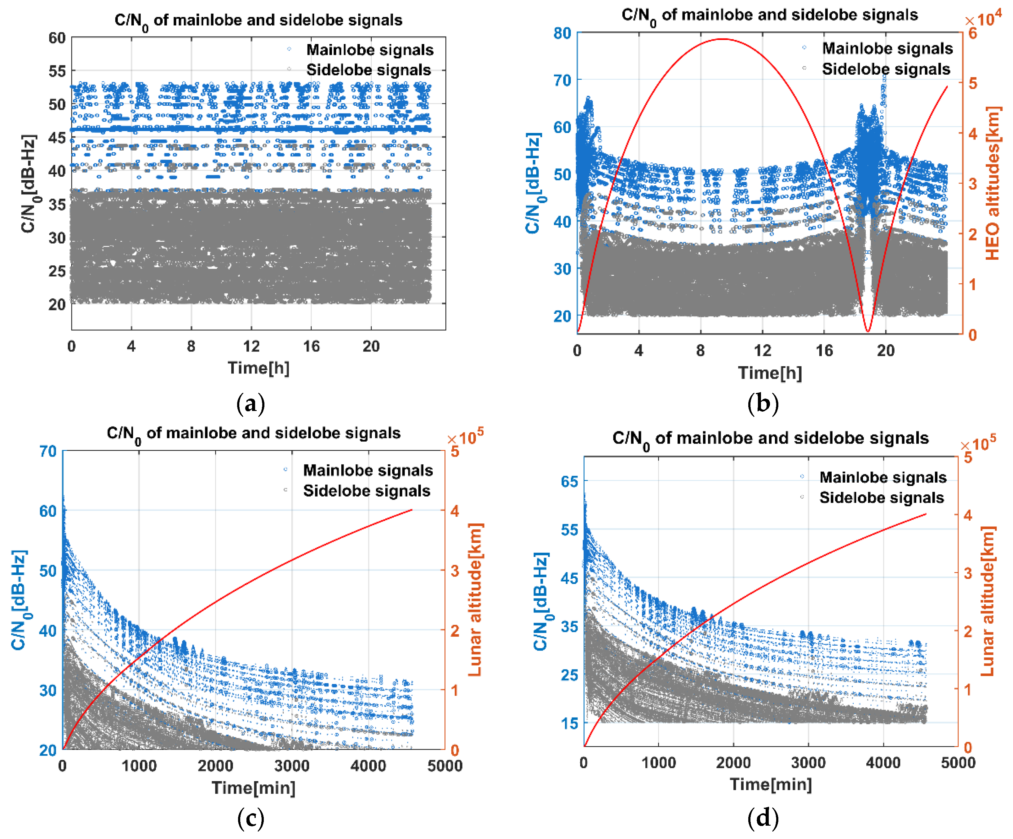
N0 is a critical parameter for spaceborne navigation since sidelobe signals are mostly received. C/N0 of GEO, HEO, and lunar trajectory are shown in Figure 7. In our paper, C/N0 was calculated using Equation (2), in which the transmission distances between GNSS satellites and spacecraft were computed using the orbits described in Table 1 and Table 3, Table 4 and Table 5. Note that we showed C/N0 of each visible GNSS satellite here. A GNSS satellite was visible once the signal was not blocked by the Earth and the C/N0 was beyond the receiver sensitivity. As the spacecraft moves along its orbit, the received signals were marked as blue or grey dots for mainlobe or sidelobe signals, respectively. The red curve in Figure 7b refers to altitudes of HEO; the red curves in Figure 7c,d refer to altitudes of lunar trajectory. Obviously, the altitude of GEO was basically the same during the simulation period, so it was not shown here. Numbers of observations from mainlobe and sidelobe signals were collected in Table 7. The simulation period of GEO, HEO, and lunar trajectory was 24, 24, and 76.2 h, respectively. The sampling rate of the three types of spacecraft was 30 s.
For the GEO spacecraft, 3 GEO and 3 IGSO satellites of BDS-3 were constantly visible. Mainlobe signal variation was between 35 and 46 dB-Hz; sidelobe signals mostly ranged between 16~32 dB-Hz. Numbers of GEO observations showed that almost 92.4% of the received signals were sidelobe signals, which is reasonable, since the altitude of GEO was higher than most of the GNSS satellites.
For the HEO spacecraft, the highest C/N0 appeared at perigee, which was as strong as 65 dB-Hz. When the spacecraft moved towards apogee, C/N0 was reduced because sidelobe signals were received. In total, 86.5% of the received signals were from sidelobe signals. HEO spaceborne antenna received more mainlobe signals than that of GEO. This was due to the low altitude near the perigee, where mostly mainlobe signals were received.
For lunar trajectory, when receiver sensitivity was set as 20 dB-Hz, 78.4% of the received signals were sidelobe signals. Due to the long transmission loss, C/N0 of most signals were below receiver thresholds. When receiver sensitivity increased to 15 dB-Hz, the received signals increased by 6.5% and 94.2% for mainlobe and sidelobe signals respectively, which will bring significant improvement in signal visibility.

3.2. Signal Visibility and GDOP

The above analysis of C/N0 indicates that abundant signal visibility of GEO and HEO spacecraft can be ensured. The satellite was visible once the nadir angle was greater than the Earth block angle and the C/N0 was beyond the receiver sensitivity. GDOP was an important index to measure the effect of the satellite geometry on the positioning and timing solution [39,40]. It can be calculated by:
G D O P = t r ( H T H ) 1
For multi-GNSS constellations, it was assumed that the measurements of all the satellites were statistically independent. Taking dual-GNSS constellation as an example, α and β is the satellites from different constellations, the matrix H is expressed as follows:
H = [ Δ x 1 α ρ 1 Δ y 1 α ρ 1 Δ z 1 α ρ 1 1 0 Δ x 2 α ρ 2 Δ y 2 α ρ 2 Δ z 2 α ρ 2 1 0 Δ x n α ρ n Δ y n α ρ n Δ z n α ρ n 1 0 Δ x 1 β ρ 1 Δ y 1 β ρ 1 Δ z 1 β ρ 1 0 1 Δ x 2 β ρ 2 Δ y 2 β ρ 2 Δ z 2 β ρ 2 0 1 Δ x m β ρ m Δ y m β ρ m Δ z m β ρ m 0 1 ]
where Δ x i = x i x , Δ y i = y i y , Δ z i = z i z ; ( x , y , z ) is the approximate position of the receiver; ( x i , y i , z i ) is the position of the i-th satellite; ρ i is the distance of the i-th satellite with respect to the receiver.
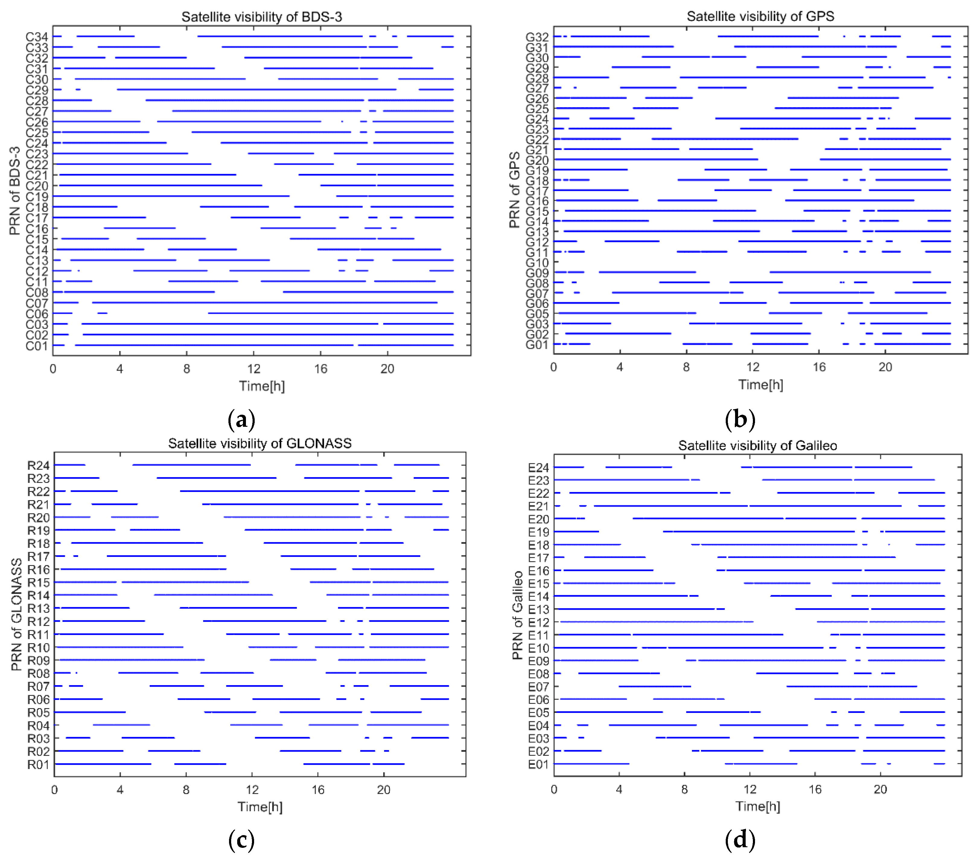
Visible satellites of the GEO spacecraft are shown in Figure 8 and Figure 9. Meanwhile, visible satellites of each GNSS constellation were calculated. For the GEO spacecraft, the mean visible satellites of BDS-3, GPS, Galileo, and GLONASS over 24 h were 25.4/21.3/19.4/19.1, respectively. Satellite visibility of BDS-3 from Figure 9 showed that GEO and IGSO satellites of BDS-3 were constantly visible. This was the reason why visible satellites of BDS-3 were more than that of GPS. Mean visible satellites of GREC combination reached 84.8.
GDOP of GEO spacecraft is shown in Figure 10. The mean GDOP of BDS-3 is 3.4. With GPS combined, it improved to 2.6, and four systems yield a mean GDOP of 2.0, which is a rather good satellite geometry. This good satellite geometry was simply benefited from the large number of visible satellites, as we have shown in Figure 8. For GEO spacecraft, the distance between the receiver and the GNSS satellites was not far enough to make serious signal attenuation; therefore, a large number of sidelobe signals could be received, leading to a large number of visible satellites.
Visible satellites of HEO spacecraft are shown in Figure 11. Visible satellites around apogee were slightly less than that of perigee, where signals from the same side and different side of the Earth were both received. We noticed that there was a sharp decrease of visible satellites at the lowest altitude of HEO, which was marked as the red circle in Figure 11. This was because the nadir angles of the spacecraft with respect to GNSS satellites were relatively small; therefore, signals from the other side of the Earth were mostly blocked. When the HEO spacecraft moved away from perigee, the altitude of the spacecraft increased and more signals from the other side of the Earth were tracked. Mean visible satellites of BDS-3, GPS, Galileo and GLONASS over 24 h were 22.9/19.8/17.0/15.9, respectively. From Figure 12a,b, we can see that three GEO satellites of BDS-3 were about 94.0% time visible during the whole simulation period. This is why the visible satellites of BDS-3 were more than that of GPS. Considering that there were 24 satellites of Galileo and GLONASS, less visible satellites from the two systems are reasonable. Since the Galileo altitude was slightly higher than GLONASS, more signals of Galileo from the other side of the Earth could be received.
GDOP of the HEO spacecraft is shown in Figure 13, it rose and fell. We obtained the best satellite geometry near perigee, and the worst satellite geometry near apogee. GDOP of BDS-3 ranged from 0.96~6.64. With GPS included, GDOP decreased to 0.71~5.30. GDOP of GREC combination varied from 0.52~4.42. Mean GDOP of BDS-3, BDS-3/GPS and GREC combination was 3.57, 2.88 and 2.3, respectively. This good satellite geometry also resulted from the large number of visible satellites. For the HEO spacecraft, nadir- and zenith-pointing antennas were mounted; therefore, good satellite visibility could be realized.
Visible satellites and GDOP of lunar probe with thresholds of 20 and 15 dB-Hz are shown in Figure 14 and Figure 15, respectively.
The lunar probe experienced larger signal attenuation than the GEO and HEO spacecraft. It received most signals near departing epochs, then the visible satellites decreased as the lunar probe was flying near the moon. We saw that, for the threshold of 20 dB-Hz, with only BDS-3 satellites involved, satellite geometry was rather poor, and the lunar probe could only track about 2 visible satellites as it was moving towards the moon. When more systems were included, the situation of sparse signal was still not improved. Mean visible satellites of BDS-3, GPS, Galileo, and GLONASS over the simulation period, i.e., 76.2 h were 7.7/ 4.9/ 3.5/ 3.1, respectively. As the receiver threshold increased to 15 dB-Hz, we could see that there was a significant increase in visible satellites. However, the satellite geometry was still poor for BDS-3 only. It improved as GPS was combined with BDS-3. When four systems were included, the GDOP decreased further and reached a maximum of 3392. Mean visible satellites of BDS-3, GPS, Galileo and GLONASS were 13.0/ 8.6/ 6.3/ 5.8, respectively. GEO and IGSO satellites of BDS-3 were 47.4% visible during the whole simulation time, which was almost twice compared with the MEO satellites from BDS-3, GPS, Galileo and GLONASS.
Unlike the GEO and HEO spacecraft, signal reception interruption was likely to happen for the lunar probe. As shown in Table 8, with a receiver threshold of 20 dB-Hz, the lunar probe could not track 1 or 4 satellites continuously for all the combinations. When mainlobe and sidelobe signals were both considered, the availability of at least 1 BDS-3 satellite was almost the same as the B2 signal in Table 8 of ref [30], in which real BDS 3D antenna patterns were used. The availability of at least 4 BDS-3 satellites was slightly higher than the results of all the signals in Table 8 of ref [30]. When the receiver threshold improved to 15 dB-Hz, the lunar probe was able to receive at least 1 satellite continuously for all the combinations. Meanwhile, BDS-3/GPS and GREC combinations were able to offer four visible satellites continuously. Due to the large GDOP of these conditions, it made no sense to discuss position, velocity, and time navigation performances, even if there were at least four visible satellites.

3.3. Navigation Performance

3.3.1. GEO Navigation Performance

The above analysis showed that, with sidelobe signals included, good GNSS satellite geometry could be provided for the GEO spacecraft. In this section, the position of the spacecraft was derived by single-epoch least square estimator. The spacecraft positions used for measurement simulation were deemed as true positions. The differences between single-epoch least-square solution and the true positions were calculated; RMSs of all the differences are listed in Table 9. We only show the differences of BDS-3 SPP here in Figure 16. For the dual-GNSS processing mode, i.e., BDS-3/GPS combination, the 3D position error decreased by 18.6% in contrast to BDS-3 only processing. For GREC combination, the SPP accuracy increased by 21.5% compared with the dual-GNSS processing. Obviously, the improvement of navigation performance resulted from the improved signal geometry. For each epoch for each satellite, code post-fit residuals were computed by the difference between the actual code measurements and the estimated distance between the satellite and the receiver; the related errors were also removed. The RMSs of code post-fit residuals were 3.75 m, 5.08 m, 4.82 m, and 5.1 m for BDS-3, GPS, BDS-3/GPS, and GREC combination, respectively. In total, 42.4% of the received signals were higher than 30 dB-Hz, and the pseudorange measurement noises were comparable to the results in [37], proving that our observation simulation routine was reliable.

3.3.2. HEO Navigation Performance

In this section, we focus on HEO navigation performance. The position strategies that applied to the HEO spacecraft were the same as those applied to the GEO spacecraft. The differences between BDS-3 SPP and nominal HEO are shown in Figure 17, and positioning RMSs are listed in Table 10. For the BDS-3/GPS combination, 3D position error decreased by 6.1% in contrast to BDS-3 only processing. Galileo and GLONASS increased SPP accuracy by 14.7% compared with dual-GNSS processing mode. The RMSs of code post-fit residuals were 3.73 m, 5.05 m, 4.8 m and 5.31 m for BDS-3, GPS, BDS-3/GPS and GREC combination, respectively. A total of 48.5% of the received signals were higher than 30 dB-Hz, which is 6.1% more than the GEO spacecraft. Therefore, lower code noises were derived. We can see that larger positioning error occurred near apogee; the trend of positioning error followed the trend of GDOP (Figure 13).

3.3.3. Lunar Navigation Performance

Considering the analysis of signal visibility in Section 3.2, all the three position schemes could not provide continuous position solutions with the threshold of 20 dB-Hz. Therefore, we only considered observations with a 15 dB-Hz threshold here. The differences of GREC SPP and nominal lunar trajectory are shown in Figure 18. We can see that very large positioning errors occurred near the end of the trajectory. RMSs in Table 11 show that the 3D position error of BDS-3/GPS combination decreased by 34.0% in contrast to BDS-3 only. This benefited from the significantly improved signal geometry. Positioning errors of the X and Y component were much larger than that of the Z component. A possible explanation for the smaller Z component was due to the high constraint in cross and along direction; the Z component was consistent with the cross direction [36]. When more systems were included, SPP accuracy only increased by 9.0% compared with the BDS-3/GPS combination. Figure 15 shows that GDOPs of GREC were only slightly smaller than that of the BDS-3/GPS combination. Therefore, a significant improvement in SPP accuracy could not be realized. The RMSs of code post-fit residuals were 5.65 m, 6.79 m, 6.99 m, and 6.86 m for BDS-3, GPS, BDS-3/GPS, and GREC combination, respectively. Among the observations, 42.3% of the received signals were below 20 dB-Hz and 84.4% were below 30 dB-Hz, resulting in higher code noise than the GEO and HEO spacecraft.

4. Discussion

Our results show that space users benefit from multi-GNSS considerably, especially for users that are far away from the Earth. Therefore, developing interoperable multi-GNSS is important. Different from terrestrial uses, GNSS antenna patterns play an important role in spacecraft positioning since sidelobe signals are mostly received. Until now, only antenna patterns of GPS Block IIR, IIR-M, IIF, and IIA were published. Research regarding BDS-3 and Galileo antenna patterns can be found in [9,30]; however, the data are unavailable. Great progress could be made once these data are published. More accurate simulation results can be provided and better suggestions regarding spaceborne receiver design could be proposed. In addition to these global positioning systems, navigation performances could be further improved once regional satellite navigation systems, such as the quasi-zenith satellite system (QZSS) from Japan, navigation with Indian constellation (NavIC) from India, and Korea Positioning System (KPS) from South Korea are used. These abundant signals will help with GNSS-based spacecraft positioning at even further distances such as halo orbits near the Earth-moon Lagrange points, contributing to deep space exploration.

5. Conclusions

To explore the navigation performance of BDS-3 and the contribution of multi-GNSS, pseudorange observations were simulated for three classical types of orbits, including GEO, HEO and lunar trajectory. Based on available GNSS transmitter antenna pattern and two receivers in nadir and zenith direction, C/N0 were calculated in order to determine the visible satellites. Number of observations show that 92.4%, 86.5% and 86.8% of the received signals are sidelobe signals for GEO, HEO and lunar trajectory, respectively (The GEO and HEO spacecraft were evaluated with a threshold of 20 dB-Hz and lunar probe with 15 dB-Hz). Even BDS-3 only can ensure a continuous navigation solution for GEO and HEO. On the other hand, to ensure a continuous navigation solution for a lunar probe, it was necessary to combine BDS-3 with GPS or other GNSS systems, with a receiver threshold of 15 dB-Hz. All three space vehicles received more BDS-3 signals, owing to the GEO and IGSO satellites. Meanwhile, Galileo provided more visible satellites than GLONASS due to the smaller Earth block angle. With only BDS-3 signals considered, mean visible satellites were 25.4 and 22.9 for the GEO and HEO spacecraft, respectively, yielding mean GDOP of 3.4 and 3.6. Combining GPS with BDS-3, the positioning accuracy increased by 18.6% and 6.1%. For the lunar probe, signal geometry was less optimistic. All the combinations cannot provide a continuous navigation solution with a receiver threshold of 20 dB-Hz. The best signal geometry was provided by the GREC combination, which produced a max GDOP of 3392 when receiver sensitivity was 15 dB-Hz.
Our investigation indicates that BDS-3 is capable of providing good navigation performance for the GEO and HEO spacecraft. For lunar missions, the SPP accuracy delivered by GREC combination was rather poor, even with 15 dB-Hz receiver thresholds. Significant improvements on SPP accuracy are hard to realize due to the high GDOP; therefore, a software receiver with an orbital filter or GNSS/INS/Star tracker integration may be necessary for lunar missions. Last but not least, the lunar mission discussed in this paper only covered the trajectory that moved from the Earth to the Moon. The realistic lunar mission included lunar orbits, final descent, and landing phase, which may require other navigation sensors or lunar navigation infrastructure; it is an interesting topic to investigate in the future.

Author Contributions

Conceptualization, M.G. and T.X.; methodology, M.G.; formal analysis, M.G., M.L., F.G. and D.M.; writing—original draft preparation, M.G.; writing—review and editing, T.X., M.L., F.G. and D.M.; funding acquisition, T.X. All authors have read and agreed to the published version of the manuscript.

Funding

This research was funded by National Key Research and Development Program of China (2020YFB0505800 and 2020YFB0505804), National Natural Science Foundation of China (41874032 and 41704018).

Institutional Review Board Statement

Not applicable.

Informed Consent Statement

Not applicable.

Acknowledgments

The authors would like to thank the Lockheed Martin Space Systems Company for publishing the GPS antenna patterns.

Conflicts of Interest

The authors declare no conflict of interest.

References

  1. Bauer:, F.H. GNSS Space Service Volume & Space User Data Update. In Proceedings of the International Committee for GNSS 10th Meeting, Boulder, CO, USA, 1 November 2015; pp. 1–6. [Google Scholar]
  2. Moreau, M.C. GPS Receiver Architecture for Autonomous Navigation in High Earth Orbits; University of Colorado at Boulder: Boulder, CO, USA, 2001. [Google Scholar]
  3. Bock, H.; Hugentobler, U.; Springer, T.A.; Beutler, G. Efficient precise orbit determination of LEO satellites using GPS. Adv. Space Res. 2002, 30, 295–300. [Google Scholar] [CrossRef]
  4. Mao, X.; Arnold, D.; Girardin, V.; Villiger, A.; Jäggi, A. Dynamic GPS-based LEO orbit determination with 1 cm precision using the Bernese GNSS Software. Adv. Space Res. 2021, 67, 788–805. [Google Scholar] [CrossRef]
  5. Filippi, H.; Gottzein, E.; Kuehl, C.; Mueller, C.; Barrios-Montalvo, A.; Dauphin, H. Feasibility of GNSS receivers for satellite navigation in GEO and higher altitudes. In Proceedings of the 2010 5th ESA Workshop on Satellite Navigation Technologies and European Workshop on GNSS Signals and Signal Processing (NAVITEC), IEEE, Noordwijk, The Netherlands, 8–10 December 2010; pp. 1–8. [Google Scholar]
  6. Kahr, E. Multi-Constellation GNSS for Absolute and Relative Navigation in Highly Elliptical Orbits; University of Calgary: Calgary, AB, Canada, 2017. [Google Scholar]
  7. Park, Y.; Won, J.H.; Kwon, K.H. Performance Analysis of Multi-Constellation and Multi-Frequency GNSS Receivers in Deep Space. In Proceedings of the 30th International Technical Meeting of the Satellite Division of the Institute of Navigation (ION GNSS+ 2017), Portland, OR, USA, 25–29 September 2017; pp. 1127–1132. [Google Scholar]
  8. Impresario, G.; D’Amore, G.; Stallo, C.; Ansalone, L.; Tuozzi, A. GNSS and GALILEO for CIS-Lunar and Moon Navigation. In Proceedings of the 2018 IEEE 4th International Forum on Research and for Society and Industry (RTSI), Palermo, Italy, 10–13 September 2018; pp. 1–5. [Google Scholar]
  9. Delépaut, A.; Giordano, P.; Ventura-Traveset, J.; Blonski, D.; Schönfeldt, M.; Schoonejans, P.; Aziz, S.; Walker, R. Use of GNSS for lunar missions and plans for lunar in-orbit development. Adv. Space Res. 2020, 66, 2739–2756. [Google Scholar] [CrossRef]
  10. Bauer, F.H.; Moreau, M.C.; Dahle-Melsaether, M.E.; Petrofski, W.P.; Stanton, B.J.; Thomason, S.; Harris, G.A.; Sena, R.P. The GPS space service volume. In Proceedings of the 19th International Technical Meeting of the Satellite Division of the Institute of Navigation (ION GNSS 2006), Fort Worth, TX, USA, 26–29 September 2006; pp. 2503–2514. [Google Scholar]
  11. Bauer, F.H.; Parker, J.J.; Welch, B.; Enderle, W. Developing a robust, interoperable GNSS space service volume (SSV) for the global space user community. In Proceedings of the 2017 International Technical Meeting of the Institute of Navigation, Monterey, CA, USA, 30 January–2 February 2017; pp. 132–149. [Google Scholar]
  12. Parker, J.J.K. Refining the GPS Space Service Volume (SSV) and Building a Multi-GNSS SSV. In Proceedings of the SCaN Workshop on Emerging Technologies for Autonomous Space Navigation, Washington, DC, USA, 16 February 2017. [Google Scholar]
  13. United Nations. The Interoperable Global Navigation Satellite Systems Space Service Volume; United Nations Office for Outer Space Affairs: Vienna, Austria, 2018. [Google Scholar]
  14. Jing, S.; Zhan, X.; Lu, J.; Feng, S.; Ochieng, W.Y. Characterisation of GNSS Space Service Volume. J. Navig. 2015, 68, 107–125. [Google Scholar] [CrossRef]
  15. Enderle, W.; Gini, F.; Boomkamp, H.; Parker, J.J.; Ashman, B.W.; Welch, B.W.; Koch, M.; Sands, O.S. Space user visibility benefits of the multi-GNSS Space Service Volume: An internationally-coordinated, global and mission-specific analysis. In Proceedings of the 31st International Technical Meeting of the Satellite Division of the Institute of Navigation (ION GNSS+ 2018), Miami, FL, USA, 24–28 September 2018; pp. 1191–1207. [Google Scholar]
  16. Yang, J.; Wang, X.; Shen, L.; Chen, D. Availability analysis of GNSS signals above GNSSs constellation. J. Navig. 2021, 74, 446–466. [Google Scholar] [CrossRef]
  17. Liu, X.; Zhan, X.; Huang, J.; Qin, C.; Chi, C. Space Vehicle Orbital Determination Performance Analysis Considering GNSS Side Lobe Signals. In Proceedings of the International Conference on Aerospace System Science and Engineering, Toronto, ON, Canada, 30 July–1 August 2019; pp. 129–145. [Google Scholar]
  18. Moreau, M.C.; Bauer, F.H.; Carpenter, J.R.; Davis, E.P.; Davis, G.W.; Jackson, L.A. Preliminary results of the gps flight experiment on the high earth orbit AMSAT-OSCAR 40 spacecraft. Adv. Astronaut. Sci. 2002, 111, 45–59. [Google Scholar]
  19. Parker, J.J.K. GPS/GNSS space service volume (SSV) update initiatives. NaSa Goddard Space Flight Cent. 2016, 40, 2016. [Google Scholar]
  20. Winkler, S.; Ramsey, G.; Frey, C.; Chapel, J.; Chu, D.; Freesland, D.; Krimchansky, A.; Concha, M. GPS receiver on-orbit performance for the GOES-R spacecraft. In Proceedings of the 10th International ESA Conference on Guidance, Navigation & Control Systems, Salzburg, Austria, 29 May–2 June 2017. [Google Scholar]
  21. Burch, J.L.; Moore, T.E.; Torbert, R.B.; Giles, B. Magnetospheric multiscale overview and science objectives. Space Sci. Rev. 2016, 199, 5–21. [Google Scholar] [CrossRef] [Green Version]
  22. Marquis, W.A.; Reigh, D.L. The GPS Block IIR and IIR-M Broadcast L-band Antenna Panel: Its Pattern and Performance. Navig. J. Inst. Navig. 2015, 62, 329–347. [Google Scholar] [CrossRef]
  23. Donaldson, J.E.; Parker, J.J.; Moreau, M.C.; Highsmith, D.E.; Martzen, P.D. Characterization of on-orbit GPS transmit antenna patterns for space users. Navig. J. Inst. Navig. 2020, 67, 411–438. [Google Scholar] [CrossRef]
  24. Meng, Y.; Qu, B.; Wang, Y.; Bian, L.; Li, L.; Wang, X. A High Sensitive GNSS Receiver for High Altitude Space Missions. In Proceedings of the 30th International Technical Meeting of the Satellite Division of the Institute of Navigation (ION GNSS+ 2017), Portland, OR, USA, 25–29 September 2017; pp. 1688–1694. [Google Scholar]
  25. Musumeci, L.; Dovis, F.; Silva, J.S.; da Silva, P.F.; Lopes, H.D. Design of a High Sensitivity GNSS receiver for Lunar missions. Adv. Space Res. 2016, 57, 2285–2313. [Google Scholar] [CrossRef]
  26. Capuano, V.; Shehaj, E.; Blunt, P.; Botteron, C.; Farine, P.A. High accuracy GNSS based navigation in GEO. Acta Astronaut. 2017, 136, 332–341. [Google Scholar] [CrossRef]
  27. Dovis, F. Autonomous orbit determination for future GEO and HEO missions. In Proceedings of the Workshop on Satellite Navigation Technologies & European Workshop on Gnss Signals & Signal Processing, IEEE, Noordwijk, The Netherlands, 8–10 September 2011. [Google Scholar]
  28. Liu, H.; Cao, J.; Cheng, X.; Peng, J.; Tang, G. The data processing and analysis for the CE-5T1 GNSS experiment. Adv. Space Res. 2017, 59, 895–906. [Google Scholar] [CrossRef]
  29. Shi, T.; Zhuang, X.; Xie, L. Performance evaluation of multi-GNSSs navigation in super synchronous transfer orbit and geostationary earth orbit. Satell. Navig. 2021, 2, 5. [Google Scholar] [CrossRef]
  30. Lin, K.; Zhan, X.; Yang, R.; Shao, F.; Huang, J. BDS Space Service Volume characterizations considering side-lobe signals and 3D antenna pattern. Aerosp. Sci. Technol. 2020, 106, 106071. [Google Scholar] [CrossRef]
  31. BeiDou, I. BeiDou Navigation Satellite System Signal in Space Interface Control Document Open Service Signal B1I (Version 3.0); China Satellite Navigation Office: Beijing, China, 2012.
  32. GLONASS. Global Navigation Satellite System GLONASS, Interface Control Document, Navigational Radio Signal in bands L1, L2; Russian Institute of Space Device Engineering: Moscow, Russia, 2008. [Google Scholar]
  33. Galileo, I. European GNSS (Galileo) Open Service Signal in Space Interface Control Document; OS SIS ICD; European Space Agency/European GNSS Supervisory Authority: Brussels, Belgium, 2015. [Google Scholar]
  34. Xie, G. Principles of GPS and Receiver Design; Publishing House of Electronics Industry: Beijing, China, 2009; Volume 7, pp. 241–244. [Google Scholar]
  35. Rebischung, P.; Griffiths, J.; Ray, J.; Schmid, R.; Collilieux, X.; Garayt, B. IGS08: The IGS realization of ITRF2008. GPS Solut. 2012, 16, 483–494. [Google Scholar] [CrossRef]
  36. Jiang, K.; Li, M.; Wang, M.; Zhao, Q.; Li, W. TJS-2 geostationary satellite orbit determination using onboard GPS measurements. GPS Solut. 2018, 22, 87. [Google Scholar] [CrossRef]
  37. Wang, M.; Shan, T.; Zhang, W.; Huan, H. Analysis of BDS/GPS Signals’ Characteristics and Navigation Accuracy for a Geostationary Satellite. Remote Sens. 2021, 13, 1967. [Google Scholar] [CrossRef]
  38. Wang, M.; Shan, T.; Li, M.; Liu, L.; Tao, R. GNSS-based orbit determination method and flight performance for geostationary satellites. J. Geod. 2021, 95, 89. [Google Scholar] [CrossRef]
  39. Nicolini, L.; Caporali, A. Investigation on reference frames and time systems in multi-GNSS. Remote Sens. 2018, 10, 80. [Google Scholar] [CrossRef] [Green Version]
  40. Teng, Y.; Wang, J.; Huang, Q. Minimum of Geometric Dilution of Precision (GDOP) for five satellites with dual-GNSS constellations. Adv. Space Res. 2015, 56, 229–236. [Google Scholar] [CrossRef]
Figure 1. GNSS constellations.
Remotesensing 14 00318 g001
Figure 2. GNSS symmetric antenna patterns.
Remotesensing 14 00318 g002
Figure 3. Physical visibility of HEO spacecraft.
Remotesensing 14 00318 g003
Figure 4. GNSS antenna coordinate system.
Remotesensing 14 00318 g004
Figure 5. Receiver antenna gain with off-boresight angles.
Remotesensing 14 00318 g005
Figure 6. Earth block angle.
Remotesensing 14 00318 g006
Figure 7. C/N0 of mainlobe and sidelobe signals for three types of spacecraft: (a) GEO; (b) HEO; (c) Lunar trajectory (20 dH-Hz); (d) Lunar trajectory (15 dH-Hz).
Remotesensing 14 00318 g007
Figure 8. Visible satellites of GEO.
Remotesensing 14 00318 g008
Figure 9. Satellite visibility of GEO spacecraft. (a) Satellite visibility of BDS-3. (b) Satellite visibility of GPS. (c) Satellite visibility of Galileo. (d) Satellite visibility of GLONASS.
Remotesensing 14 00318 g009
Figure 10. GDOP of GEO spacecraft.
Remotesensing 14 00318 g010
Figure 11. Visible satellites.
Remotesensing 14 00318 g011
Figure 12. Satellite visibility of HEO. (a) Satellite visibility of BDS-3. (b) Satellite visibility of GPS. (c) Satellite visibility of Galileo. (d) Satellite visibility of GLONASS.
Remotesensing 14 00318 g012
Figure 13. GDOP of HEO spacecraft.
Remotesensing 14 00318 g013
Figure 14. Visible satellites and GDOP of lunar probe with 20 dB-Hz threshold.
Remotesensing 14 00318 g014
Figure 15. Visible satellites and GDOP of lunar probe with 15 dB-Hz threshold.
Remotesensing 14 00318 g015
Figure 16. Differences between BDS SPP and the nominal GEO.
Remotesensing 14 00318 g016
Figure 17. Differences between BDS SPP and the nominal HEO.
Remotesensing 14 00318 g017
Figure 18. Differences between GREC SPP and the nominal lunar trajectory.
Remotesensing 14 00318 g018
Table 1. Parameters of GNSS Constellations.
SystemGPSBDSGLONASSGalileo
Orbital typeMEOGEOIGSOMEOMEOMEO
Number of satellites3133242424
Constellation configurationW31/6/1Placed at East longitude 80°, 110.5° and 140°Placed at East longitude 0°, 120° and 240°W24/3/1W24/3/1W 24/3/1
Inclination55°055°55°64.8°56°
Altitudes [km]20,20035,78635,78621,52819,10023,221.7
Table 2. GNSS Frequency.
SystemFreq. Band/Frequency [MHz]
GPSL1/1575.42
BDSB1I/1575.42
GLONASS *L1/ 1602 *
GalileoE1/1575.42
* In this simulation GLONASS frequency band is simplified to 1602 MHz.
Table 3. GEO Parameter *.
Altitudes [km]EccentricityInclination (°)RAAN (°)Argument of Perigee (°)True Anomaly (°)
GEO35,78600000
* Epoch: 20 May 2021 00:00:00–21 May 2021 00:00:00 (UTC).
Table 4. HEO Parameter *.
Semi-Major Axis (km)EccentricityInclination (°)RAAN (°)Argument of Perigee (°)True Anomaly (°)
HEO35,937.50.808763.402700
* Epoch: 20 May 2021 00:00:00–21 May 2021 00:00:00 (UTC).
Table 5. Lunar trajectory Parameter *.
Semi-Major Axis (km)EccentricityInclination (°)RAAN (°)Argument of Perigee (°)True Anomaly (°)
Start67,500.440.896831181179.8357.8
Stop294,807.1820.994443.168174.6175.8175.94
* Epoch: 20 May 2021 22:48:00–24 May 2021 03:00:00 (UTC).
Table 6. Earth block angles of different system orbit.
System OrbitGPS
MEO
BDSGalileo
MEO
GLONASS
MEO
MEOIGSO/GEO
Earth block angle [deg]13.8413.218.7012.2814.50
Table 7. Number of observations from mainlobe and sidelobe signals.
Mainlobe SignalSidelobe Signal
GEO18,502226,155
HEO29,143186,635
Lunar trajectory (20 dB-Hz)18,97768,864
Lunar trajectory (15 dB-Hz)20,299133,767
Table 8. Satellite visibility of different system combinations.
Receiver Thresholds (dB-Hz)SystemsAt Least 1 SatelliteAt Least 4 Satellites
20BDS-393.9%58.9%
BDS-3/GPS97.7%65.0%
GREC99.4%79.3%
15BDS-3100%99.0%
BDS-3/GPS100%100%
GREC100%100%
Table 9. RMS of Position with different system combinations.
Position (m)BDS-3BDS-3/GPSGREC
X12.710.48.2
Y12.09.87.7
Z2.72.11.6
3D17.714.411.3
Table 10. RMS of Position with different system combinations.
Position (m)BDS-3BDS-3/GPSGREC
X7.46.96.1
Y10.39.48.1
Z19.418.215.5
3D23.121.718.5
Table 11. RMS of Position with different system combinations.
Position (km)BDS-3BDS-3/GPSGREC
X2.4192.0531.779
Y3.5402.0161.914
Z0.4710.2910.276
3D4.3132.8922.628
Publisher’s Note: MDPI stays neutral with regard to jurisdictional claims in published maps and institutional affiliations.

