Article

Estimation of Individual Tree Biomass in Natural Secondary Forests Based on ALS Data and WorldView-3 Imagery

1
School of Forestry, Northeast Forestry University, Harbin 150040, China
2
Key Laboratory of Sustainable Forest Ecosystem Management-Ministry of Education, Northeast Forestry University, Harbin 150040, China
3
Department of Environmental Resources Engineering, State University of New York College of Environmental Science and Forestry, Syracuse, NY 13210, USA
*
Author to whom correspondence should be addressed.
Remote Sens. 2022, 14(2), 271; https://doi.org/10.3390/rs14020271
Submission received: 16 December 2021 / Accepted: 4 January 2022 / Published: 7 January 2022

Abstract

:
Individual-tree aboveground biomass (AGB) estimation can highlight the spatial distribution of AGB and is vital for precision forestry. Accurately estimating individual tree AGB is a requisite for accurate forest carbon stock assessment of natural secondary forests (NSFs). In this study, we investigated the performance of three machine learning and three ensemble learning algorithms in tree species classification based on airborne laser scanning (ALS) and WorldView-3 imagery, inversed the diameter at breast height (DBH) using an optimal tree height curve model, and mapped individual tree AGB for a site in northeast China using additive biomass equations, tree species, and inversed DBH. The results showed that the combination of ALS and WorldView-3 performed better than either single data source in tree species classification, and ensemble learning algorithms outperformed machine learning algorithms (except CNN). Seven tree species had satisfactory accuracy of individual tree AGB estimation, with R2 values ranging from 0.68 to 0.85 and RMSE ranging from 7.47 kg to 36.83 kg. The average individual tree AGB was 125.32 kg and the forest AGB was 113.58 Mg/ha in the Maoershan study site in Heilongjiang Province, China. This study provides a way to classify tree species and estimate individual tree AGB of NSFs based on ALS data and WorldView-3 imagery.

1. Introduction

Forests are essential resources and require sustainable management approaches to monitor forest structures and understand the impacts of global climate change on terrestrial ecosystems. Forest biomass is defined as the total dry weight of organic material, both aboveground and belowground, in forests. Aboveground biomass (AGB) is the sum of the dry weight of stems, branches, and foliage above the ground surface [1] and plays a vital role in carbon stock assessment and the carbon cycle [2,3,4]. Due to anthropogenic deforestation, the biomass of natural secondary forests (NSFs) in northeastern China has changed considerably in the past decades [5]. The accurate estimation of forest biomass has substantial significance in understanding the ecological and global changes [6].
There are three main methods of estimating forest biomass: physiological model-based simulation [7], measurements from traditional field survey data [8], and inversion from remote sensing datasets [9,10]. Physiological model-based simulation methods usually estimate forest biomass at local or regional scales and rely on various input variables (e.g., radiation, climate conditions, and altitude) [11]. Forest resource survey methods (e.g., direct destructive harvest measurement or indirect allometric equation models) are the primary sources of forest AGB measurement and provide accurate information for the dynamic management and planning of forest resources [12]. National Forest Inventory (NFI) programs often rely upon the plot-based field inventory and monitoring of forest conditions (e.g., forest structure, composition, biomass, and carbon) [13]. However, field survey methods are commonly laborious, enormously time-consuming, destructive, and expensive. Thus, the data obtained at field survey points are only suitable for small study areas.
Remote sensing can serve as a non-destructive alternative for more robust, continuous, and spatially explicit biomass assessment than traditional forest resource survey methods [14]. Remote sensing-based AGB estimation can provide a practical and economical approach to forest surveys and ensure the spatial integrity and time consistency of data with high precision [15]. Therefore, remote sensing technologies have been extensively applied for rapid, periodic forest biomass estimates over large areas [16]. Over the last decades, the retrieval of forest AGB (or forest biomass hereafter) based on remote sensing data has received increasing attention in both the forestry and remote sensing fields [17,18,19]. Consequently, a variety of passive and active remote sensing data have been used to estimate forest AGB [20,21,22,23]. However, both optical and microwave data suffer from challenges due to the insensitivity and saturation of the signals at medium and high biomass levels [24]. For example, Le Toan et al. concluded that in different temperate, boreal, and tropical forests, the saturation of AirSAR and E-SAR occurs at around 30, 50, and 150–200 Mg/ha in the C, L, and P bands, respectively [25]. Spectral reflectance values are insensitive to biomass changes in dense and multi-layer forest canopies, which leads to saturation of optical remotely sensed data with relatively low biomass ranges [26].
Light detection and ranging (LiDAR) is an effective technique for estimating forest biomass [27]. With a tendency not to saturate even at high biomass levels (>1000 Mg/ha) [28], LiDAR is widely used to estimate forest biomass [29,30,31]. Researchers have also demonstrated that biomass estimation accuracy can be improved by combining LiDAR and passive imagery compared to using the LiDAR data alone. For example, Luo et al. estimated forest AGB, underground biomass (BGB), and total biomass (TB) by combining LiDAR and hyperspectral data [32]. In comparison to LiDAR metrics alone, the fused data improved R2 by 5.8%, 2.2%, and 2.6%, decreased Akaike information criterion (AIC) values by 1.9%, 1.1%, and 1.2%, and reduced the root mean square error (RMSE) by 8.6%, 7.9%, and 8.3% for BGB, AGB, and TB, respectively. To explore AGB estimation at an individual tree level, researchers have also combined high-spatial-resolution imagery (e.g., QuickBird and WorldView) with LiDAR data [33,34]. LiDAR can detect three-dimensional (3-D) forest structures, so it has particular value for detecting individual tree canopies [35]. The application and development of LiDAR on individual tree crown delineation (ITCD) technology provides a reliable basis for species identification and parameter estimation (e.g., height, diameter at breast height (DBH), and AGB) at an individual tree level. Researchers have found that the accuracy of vegetation type classification can be significantly improved by combining LiDAR data with passive optical images [36], which is important because distinguishing vegetation types can be an effective method to improve biomass estimation accuracy [37,38]. For example, Chen et al. integrated airborne LiDAR data and vegetation types derived from aerial photographs for biomass mapping and concluded that incorporating species types reduced the RMSE by 10% [37]. Zhu et al. quantified the differences in accuracy of AGB estimation between results obtained with and without consideration of species type using Worldview-2 images and field surveys [39]. However, this study involved only two types of mangrove species (Sonneratia apetala and Kandelia candel) at the species level. Few studies have explored the impact of tree species on the accuracy of AGB estimation at an individual tree level within stands with the more abundant tree species that are typical in NSFs. Even so, accurate tree species classification is critical to estimate AGB at the individual tree level. The classification algorithm and the data source jointly determine classifier performance across different tree species types [40]. In recent years, the extensive use of machine learning algorithms has contributed significantly to tree species classification. There are various widely used algorithms, such as random forest (RF) [41], support vector machine (SVM) [42], convolutional neural network (CNN) [43], and extreme gradient boosting (XGboost) [44]. However, the stacking algorithm in the ensemble algorithm is rarely used for individual tree species classification.
Despite the potential for improved biomass estimation at the individual tree level, few published studies estimate individual tree AGB of NSFs in China using multi-source remote sensing data. Compared to an area-based approach, individual tree AGB estimation based on tree species classification can provide spatially explicit AGB distributions and a clear understanding of the AGB distribution of each tree species. It is crucial to consider the value of combining traditional harvesting methods with remote sensing technology to estimate AGB for individual trees, which not only takes advantage of the high accuracy of allometric growth equations, but also has the potential to accurately map the spatial distribution of biomass based on individual trees. This synergistic approach produces a large amount of data and detail expression, which paves the way for precision forestry and is also suitable for management decision-making in small or specific areas [33].
Although researchers have incorporated tree species and allometric growth equations to estimate the AGB of individual trees for specific environments [33], it has not been fully investigated in NSFs of China, especially in terms of estimating and mapping individual tree scale AGB. Since NSFs have complex structures, they pose difficulties for individual tree parameter estimation (e.g., DBH) and tree species classification. This research aims to determine if ensemble learning algorithms can improve the accuracy of tree species classification of NSFs compared to classic machine learning algorithms. In addition, we will investigate whether the integration of tree species with individual parameters (e.g., DBH) will support the fine-scale mapping of AGB in NSFs. The objectives of this study are to: (1) investigate the effects of different features in tree species classification based on Airborne Laser Scanning (ALS) data and WorldView-3 imagery, (2) explore the performance of ensemble learning algorithms in classifying tree species of NSFs, (3) estimate AGB for individual trees and evaluate the estimation accuracy, and (4) map the spatial distribution of AGB at the individual tree scale. An individual tree AGB map with sufficient resolution could highlight spatial details and provide reliable data to support subsequent research and forest management decision-making for the NSFs of China.

2. Materials and Methods

2.1. Overview of the Proposed Methodology

We implemented a five-step methodology to investigate the effect of ensemble learning algorithms and features from different data sources on tree species classification and to evaluate the accuracy of individual tree AGB estimation of various tree species: (1) data preprocessing, (2) individual tree delineation using a region-hierarchical cross-sectional analysis (RHCSA) algorithm, (3) feature extraction and selection, (4) tree species classification using machine and ensemble learning models, and (5) individual tree AGB estimation and mapping. A flowchart summarizing these five steps is provided in Figure 1.

2.2. Study Area

The 3282 ha study area is located in the Maoershan Experimental Forest Farm, Shangzhi City, Heilongjiang Province, China (see Figure 2), which ranges from 127°29′E to 127°44′E and from 45°14′N to 45°29′N. The terrain is mountainous, rising from south to north with an average elevation of about 300 m. The study area has a temperate continental monsoon climate, with an average annual temperature and annual precipitation of 2.4 °C and 700 mm, respectively. Maoershan is a typical natural secondary forest in northeastern China and is dominated by various broad-leaved trees, such as Manchurian ash (Fraxinus mandshurica Rupr.), Amur cork-tree (Phellodendron amurense Rupr.), Manchurian walnut (Juglans mandshurica Maxim.), white birch (Betula platyphylla Suk.), Mongolian oak (Quercus mongolica Fisch. ex Ledeb.), elm (Ulmus pumila L.), Korean aspen (Populus davidiana), Miyabe maple (Acer miyabei Maxim.), and lilac (Syringa oblata Lindl.), with a few coniferous trees, such as Korean pine (Pinus koraiensis Sieb. et Zucc.) and Changbai larch (Larix olgensis Henry).

2.3. Data and Preprocessing

2.3.1. Field Inventory Data

This study used inventory data of 12 sample plots dominated by the main tree species of the study area obtained in 2019. Nine sample plots were 0.09 ha (30 m × 30 m) and three sample plots were 1 ha (100 m × 100 m). In total, the parameters of 4058 trees were measured, including DBH (cm), tree height (m), and crown width (CW) (m). The tree species, location, and health of trees were recorded. DBH was measured using a perimeter ruler with a starting diameter of 5 cm. Tree height was measured using the Vertex IV ultrasound instrument system, and the location of each tree was recorded using a real-time kinematic global positioning system receiver with positional error estimated to be within 5 cm. Descriptive statistics for the main tree species in the 12 sample plots are listed in Table 1.

2.3.2. ALS Data and Preprocessing

The ALS data used in the study were acquired on September 2015 using the LiCHy airborne observation system designed by the Chinese Academy of Forestry (CAF) and mounted on a fixed-wing aircraft. The system was equipped with a LiDAR sensor (RIEGL LMS-Q680i) with data collected at an average flight altitude of 1200 m above ground level and an average speed of 65 m/s. This system generated laser beams with a wavelength of 1550 nm wavelength, a beam divergence of 0.5 mrad, a laser pulse duration of 3 ns, a laser pulse repetition rate of 200 kHz, and a scan width of 60° perpendicular to the flight direction. The average point density within each plot was 8.1 pts/m2 (min = 6.3 pts/m2, max = 11.0 pts/m2, and σ = 1.5 pts/m2).
The ALS data preprocessing included: (1) noise elimination, (2) classification of ground and non-ground points, (3) canopy height model (CHM) generation, and (4) CHM filling and smoothing. Noise elimination removed the effect of noise points such as air points, low points, and isolated points. Point cloud filtering classified the raw LiDAR points cloud into non-ground and ground points. We used kriging to generate a digital elevation model (DEM) and digital terrain model (DTM) from the LiDAR ground points and non-ground points, respectively, and then generated a CHM with 0.25 m × 0.25 m based on the difference between the DTM and the DEM. This ALS data processing was implemented using GreenValley International’s LiDAR 360 V5.1. To fill the CHM, we applied a semi-automatic hole-filling algorithm [45]. To mitigate potential invalid values and outliers, the CHM was smoothed using a Gaussian filter with a window size of 3.

2.3.3. WorldView-3 Imagery and Preprocessing

WorldView-3 imagery data were obtained on 9 September 2017 from a fourth-generation Digital Globe satellite. The image had cloud cover of 0.8%, a sun elevation angle of 49.0°, and a sun azimuth angle of 163.1°. It comprised four multispectral bands (red, green, blue, and near-infrared) with 2 m spatial resolution and one panchromatic band with 0.5 m spatial resolution.
The preprocessing of the WorldView-3 imagery, including radiometric calibration and the atmospheric correction, was implemented using ENVI 5.3 software. The Fast Line-of-sight Atmospheric Analysis of Spectral Hypercube (FLAASH) radiative transfer model was implemented for atmospheric correction and conversion to surface reflectance in the ENVI environment. After preprocessing the WorldView-3 imagery, histogram equalization was applied to adjust image brightness values. Panchromatic bands and multispectral were fused to improve the nominal spatial resolution of the multispectral imagery. The fused imagery was matched to the CHM using the relative geographic referencing with a matching error of less than 1 pixel (0.5 m).

2.4. Individual Tree Crown Delineation

This study applied the region-hierarchical cross-sectional analysis (RHCSA) algorithm to segment individual trees. This approach is less affected by forest type or crown size, and has adaptability to the typical NSFs in northeastern China [46]. Similar to other ITCD algorithms (e.g., watershed) [47] and level sets [48], the RHCSA algorithm considers tree canopies as a continuous 3-D topographic surface where a tree crown manifests as a mountain-like uplift on the CHM. The vertices of the tree are equivalent to mountaintops, with height decreasing continuously from the treetop to the boundary of the crown. The CHM was scanned horizontally from top to bottom with a fixed height threshold, and multiple cross-sections were generated for each layer. We determined whether each cross-section appeared for the first time or was produced by multiple intersecting tree crowns. Cross-sections that were generated by multiple trees were divided from high to low. This process was repeated to find the lowest heights of the CHM. The details of the RHCSA were described in [46].
The ITCD accuracy assessment considers correspondence between delineated crowns and reference crowns on a location-by-location basis [35]. From the two perspectives of detected crowns and reference crowns, crown matching considers both the overlapped crown area and the position of treetops. From the reference crown perspective, accuracy metrics reflect how well the reference crowns are detected and delineated, while the detected crown perspective reflects whether detected crowns are represented by reference crowns [46]. To best delineate the reference crowns, rather than the visual interpretation method used in many prior studies, reference crowns were generated in ArcGIS 10.2 (Esri, Redlands, CA, USA) based on the crown sizes and the locations recorded in the field. The individual tree crown matching from the detected crown perspective and the reference crown perspective was statistically evaluated. Producer’s accuracy (PA), user’s accuracy (UA), and overall accuracy (OA) metrics were also used to assess the detection accuracy:
P A = N p m + N p u m N R e f
U A = N u m + N u n m N D e t
O A = 2 × P A × U A P A + U A
where OA is overall accuracy, Npm and Npnm represent the number of 1:1 matches and near-matches from the reference crown perspective, respectively, NRef represents the total number of reference crowns, Num and Nunm represent the number of 1:1 matches and near-matches for the detected crown perspective, respectively, and NDet represents the total number of detected crowns. The matching relationship between the reference crowns and the detected crowns is shown in [35].

2.5. Tree Species Classification

We used the LiDAR-based individual tree crown segmentation results (1:1 matches and near-matches from both the reference and detected crown perspectives) as classification objects to conduct an object-based classification. Then, we extracted spectral features (8), texture features (28), and vegetation indices (8) from the WorldView-3 data, and height features (92), intensity features (92), and canopy features (3) from the ALS point cloud. To investigate the effects of different algorithms on individual tree species classification, three machine learning algorithms and three ensemble learning algorithms were applied and compared using the three feature sets (WorldView-3 features, ALS features, and WorldView-3 + ALS features). The results of individual-tree species classification provided the basis for subsequent individual-tree AGB estimation.

2.5.1. Classification System and Sample Selections

We classified the main tree species identified in the Fifth Forest Resources Inventory for the Maoershan Experimental Forest Farm for the 12 plots measured in the field. In the classification system, we accounted for sample size and the separability of tree species categories. We considered the major tree species (e.g., white birch, Changbai larch, and Korean pine), which are widely distributed, and grouped minor tree species (e.g., Miyabe maple, and lilac) together.
Based on stratified sampling, a representative and evenly distributed sample was selected using tree species as strata. This classification system consisted of seven categories with sample sizes as follows: white birch (280), Manchurian walnut (247), Manchurian ash (152), elm (314), Korean pine (352), Changbai larch (171), and others (205), with the latter including all other tree species sampled. A 10-fold cross-validation method was used to test the classification accuracy. The region of interest (ROI) was manually sketched based on the location of the individual tree and crown width in ArcGIS 10.2.

2.5.2. Feature Extraction and Selection

A total of 44 feature variables were extracted from WorldView-3 data: eight spectral features, 28 texture features, and eight vegetation indices. We extracted eight feature variables from the mean and standard deviation of the grayscale values of four bands (red, green, blue, and near-infrared) using 3 × 3 windows. As a higher-order texture feature, the Gray-Level Co-occurrence Matrix (GLCM) [49] reflects the frequency of different combinations of gray levels at various distances and directions on the image. We extracted 28 GLCM texture features, including the mean, variance, homogeneity, second moment, correlation, entropy, and contrast, for the four image bands (red, green, blue, and near-infrared). Additionally, eight vegetation indices were extracted, including the normalized vegetation index (NDVI), the difference vegetation index (DVI), the perpendicular vegetation index (PVI), the triangular vegetation index (TVI), the modified simple ratio vegetation index (MSR), the atmospherically resistant vegetation index (ARVI), the ratio vegetation index (RVI), and the enhanced vegetation index (EVI) [50].
To eliminate the effects of low shrubs, values above 2 m in the CHM were defined as vegetation hit points [51]. LiDAR height metrics based on the distribution of all returns, such as the mean, standard deviation, minimum, maximum, variance, coefficient of variation, bias, kurtosis, and accumulated height quantile, as well as the height percentile with 5% intervals, were calculated from the ALS data (46 features). Given the value of intensity and echo width distribution for tree species classification in prior studies [52], we also calculated intensity metrics of all returns such as the mean, standard deviation, minimum, maximum, variance, coefficient of variation, bias, kurtosis, accumulated intensity quantile, and intensity percentile with 5% intervals (46 features). In addition, we classified the first or single returns and calculated all features of the first-or-single returns [53]. Three more canopy metrics were calculated, including the canopy cover [54], leaf area index (LAI) [55], and gap fraction [55]. With this combination of metrics, a total of 187 LiDAR features, including 92 features of the first returns, 92 features of all returns, and three canopy features, were extracted.
Previous studies have found that feature selection algorithms are effective for avoiding the dimensional curse [56] or the Hughes effect [57] and improving classification performance [40]. RF filters have achieved good results for feature selection to reduce data redundancy and require two parameters: the number of decision trees (n_estimators) and random_state. We set n_estimators to 1000 and random_state to 10 using python 3.7 and machine learning libraries. We used the Mean Decrease Accuracy (MDA) to assess variable importance. MDA considers the impact of removing individual variables on RF accuracy, i.e., the variable with a more significant decrease in accuracy contributes more to the classification than other variables.

2.5.3. Classification Algorithms

To test the performance of tree species classification with different features and algorithms, ensemble learning algorithms (i.e., Boosting, Bagging, and Stacking), and machine learning algorithms (SVM, KNN, and Convolutional Neural Networks (CNN)) were implemented based on three sets of features (WorldView-3 features, ALS features, and WorldView-3 + ALS features). We executed these algorithms using the machine learning package (Sklearn) and the deep learning package (Tensorflow) in python 3.7.
  • SVM: SVM is a generalized linear classifier that performs binary classification of data in a supervised learning manner, where the decision boundary is the hyperplane of maximum margins solved for the learned samples [58]. SVM can perform nonlinear classification by a kernel method; the parameters of this study were set as kernel = ‘linear’.
  • KNN: The KNN method is a multivariate nonparametric algorithm that uses a set of predictor feature variables (X) to match each target pixel to a number (k) of the most similar nearest neighbor reference pixels for which values of response variables (Y) are known [59]. This study set the number of nearest neighbors to 5 with uniform weight.
  • CNN: CNN, first developed in 1995 for the classification of handwritten images [60], is a representative deep learning algorithm. CNN interprets spatial data by scanning with a series of trainable moving windows and has the capability of representation learning in a translation-invariant manner according to its hierarchical structure. In this study, the CNN had a simple structure with an input layer, two hidden layers, and an output layer, and was implemented using an epoch of 1000 and a batch size of 60.
  • Boosting: The idea of the boosting algorithm is that for a complex task, the result of multiple learners’ judgment will be better than that of a single learner. Representative boosting algorithms include adaptive boosting, the gradient boosting decision tree (GBDT), and XGBoost. XGBoost, which is an improvement of the GBDT algorithm [61], was used in this study. The main characteristics of this algorithm are (1) prevention of overfitting by regularization terms, a (2) loss function with first-order derivative and second-order derivatives, and (3) faster-running speed. The classification function was set to “multi: softmax”, the depth of the tree was set to 5, and the learning rate was 0.5.
  • Bagging: The RF classifier is a bagging approach that combines multiple decision trees [62]. RF has excellent reported classification performance, requires little human intervention, has fast computational speed, is not predisposed to overfitting, and is robust in dealing with noisy data. The parameters of this study were set as follows: the number of trees was 1000 and the random state was set to 10.
  • Stacked generalization (SG): Stacking or SG differs from bagging and boosting in two ways. First, stacking usually considers heterogeneous learners (combining different learning algorithms), while bagging and boosting mainly consider homogeneous learners. Second, stacking combines base models with meta models, while bagging and boosting combine weak learners based on deterministic algorithms. Stacking is an ensemble framework for two-layer models. The first layer (base model) consists of several base models, using the original data as model input data to obtain the prediction structure; the second layer (meta model) uses the prediction results of the first layer model as input data for retraining, which constitutes the complete stacking model [50]. We adopted SVM, KNN, and CNN as the base models, and then retrained the models using their predicted values as the input values of the meta model.

2.5.4. Accuracy Assessment

The user accuracy (UA), producer accuracy (PA), and overall accuracy (OA) were used to assess the classification accuracy. The equations were shown as follows:
U A i = N i i N i +
P A i = N i i N + i
O A = i = 1 k N i i N
where N represents the total number of samples; Nii is the number of samples assigned to the correct category; Ni+ and N+i are the number of samples predicted to be in category i and the number of samples in category i, respectively.

2.6. Estimation of Individual Tree AGB

2.6.1. Individual-Tree DBH Inversion

To estimate individual-tree AGB, it is necessary to produce an inverse of DBH based on tree height. In temperate coniferous and broad-leaved mixed forests, commonly used tree height curve models are roughly divided into the nine types shown in Table 2. Based on field inventory data, tree height curve models of seven tree species types were analyzed using R. Then, the accuracy of the nine models was compared, and the best model was selected to inverse DBH. Subsequently, we utilized the individual detected trees to verify the accuracy of the DBH inversion.
The coefficient of determination (R2) and RMSE were used to assess the goodness-of-fit of models with calculation formulas as follows:
R 2 = i = 1 n ( y ^ i y ¯ ) 2 i = 1 n ( y i y ¯ ) 2
R M S E = 1 n i = 1 n ( y i y ^ i ) 2  
where y i represents the measured DBH;   y ¯ represents the mean of the measured DBH; y ^ i represents the predicted DBH; n represents the number of samples.

2.6.2. AGB Estimation for Individual Trees

Based on the inversion of the optimal tree height curve model for each tree species, an individual-tree DBH map was obtained. Then, we estimated the biomass of the stems, branches, and foliage parts of individual trees using species-specific additive biomass equations [63,64] for northeastern China (Table 3). Finally, individual tree AGB was calculated based on the sum of the stems, branches, and foliage biomass of different tree species in the 12 sample plots. The additive biomass equations follow the structure below:
{ ln W s = a s * + b s * ln D + ε s ln W b = a b * + b b * ln D + ε b ln W f = a f * + b f * ln D + ε f ln W a = ln ( W s + W b + W f ) = ln ( a s D b s + a b D b b + a f D b f ) + ε a
where Wa, Ws, Wb, and Wf represent aboveground biomass, stem biomass, branch biomass, and foliage biomass (kg), respectively; D represents diameter at breast height (cm); ln is the natural logarithm; i = [s, b, f], representing stem, branch, and foliage, respectively; ε i is the error term; ai, bi, ai*, and bi* are regression coefficients, which are listed in Table 3 for different tree species and components.

3. Results

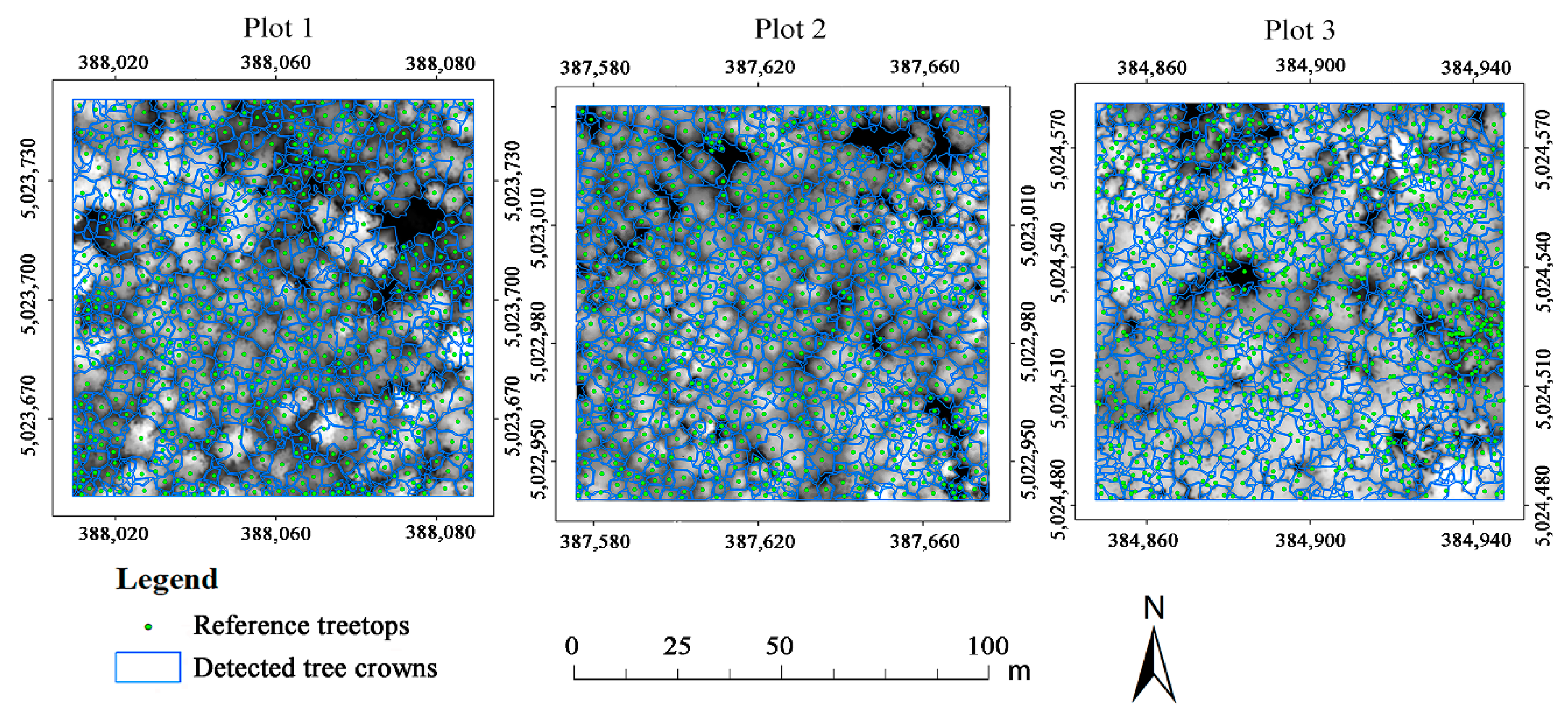
3.1. Individual Tree Crown Delineation

Accurately detecting the location and number of trees is critical for estimating AGB at the individual tree level. Since RHCSA was based on CHM for individual tree crown delineation, the resolution of the CHM had a significant impact on the results. Accordingly, this study investigated the effect of the spatial resolution of CHM on the individual tree detection rate and the overall accuracy of the RHCSA algorithm, with the goal of determining the optimal resolution where the numbers of detected individual trees best matched the counts in the field and the overall accuracy was highest. We found (Figure 3a) that when the CHM resolution was 0.25 m, the detection rate was close to 100%, which means that the total number of detected tree crowns using the RHCSA algorithm was closest to the actual numbers of individual trees in the three sample plots. Figure 3b shows that the OA of individual tree matching initially improved with increasing CHM resolution (0.5 m–0.25 m), but OA began to gradually decline with further increases in resolution (0.25 m–0.1 m). Thus, the 0.25 m spatial resolution CHM was adopted for the RHCSA algorithm in this study.
We applied the RHCSA algorithm to detect individual trees in the 0.25 m CHM and detected 2.9 million individual trees in the study area. We used the three 100 m × 100 m sample plots (2688 trees in total) to assess the accuracy of individual tree crown delineation. Figure 4 illustrates the individual treetops detected using the RHCSA algorithm (blue lines) with green points representing reference treetops.
Based on the matching conditions listed in [35], PA, UA, and OA were calculated and the accuracy assessment results for the three plots are shown in Table 4. The field inventories of the three sample plots measured 2688 trees, while the RHCSA algorithm detected 2648 trees with a detection rate of 98.51% and an average match rate (including 1:1 matches and near-matches) of 72.3%. The highest match rate was obtained in Plot 2, possibly due to the presence of fewer small trees, which were suppressed by taller trees in other plots. The least accurate match rate was obtained in Plot 3, which may be due to the uneven and very dense distribution of trees in Plot 3.

3.2. Feature Selection and Accuracy Assessment of Tree Species Classification

3.2.1. Feature Selection

After extracting feature variables from ALS data and WorldView-3, we selected the greatest contributing variables using the RF algorithm and used MDA to rank the variables. In general, the number of features can be determined as the square root of the total number of features. This process led to the selection of 13 ALS feature variables to participate in tree species classification (Figure 5).
To ensure the consistency of the number of WorldView-3 and ALS features and eliminate the influence of the number of features on algorithm comparison, we also selected 13 WorldView-3 features (Figure 6).

3.2.2. The Performance of Machine Learning Algorithms in Tree Species Classification

We tested the classification performance for three machine learning methods (SVM, KNN, and CNN) based on three sets of features (WorldView-3 features, ALS features, and WorldView-3 + ALS features).
The WorldView-3 features performed better than the ALS features for tree species classification with the SVM and KNN algorithms when the feature sets were considered independently. The combination of the ALS features and WorldView-3 features outperformed the single feature sets, which indicated the advantage of simultaneously applying LiDAR and passive imagery in tree species classification. Table 5 shows that the CNN classifier had the best performance of the three classifiers regardless of features included, while the SVM classification had the worst performance.

3.2.3. The Performance of Ensemble Learning Algorithms in Tree Species Classification

Table 6 shows the performance of the ensemble learning algorithm for tree species classification. Regardless of the features, the accuracy of the ensemble algorithms was slightly higher than that of the machine learning algorithms for tree species classification. The three ensemble algorithms showed some differences under different features: the RF algorithm had the highest classification accuracy (OA = 61.7%) with WorldView-3 features; the SG (CNN) algorithm was the best with ALS features and WorldView-3 + ALS features.
The classification performance of the combination of WorldView-3 features and ALS features was superior to a single feature set with the ensemble learning algorithms, except for the RF, where the WorldView-3 features alone achieved similar accuracy. It is worth noting that the CNN algorithm had only slightly lower classification accuracy (OA = 72.8%) than SG (CNN) (OA = 75.0%) with the combination of WorldView-3 features and ALS features, which was higher than the other ensemble learning algorithms.
We selected the best performing algorithm and features (SG (CNN) algorithm and WorldView-3 features + ALS features) and calculated a confusion matrix (Table 7) showing the classification accuracy of each tree species. The PA and UA ranged from 66.9% to 82.1% and from 67.0% to 84.2%, respectively. The highest PA was Manchurian walnut (82.1%) and the lowest PA was elm (66.9%). The highest UA was elm (84.2%) and the lowest UA was Manchurian ash (67.0%). The latter situation was caused by high misclassification between Manchurian ash and elm.

3.3. The Estimation and Assessment of Individual Tree AGB

3.3.1. Individual Tree DBH Inversion

We fitted tree height curve models for the seven tree species categories. Table 8 shows the optimal model for each tree species. For Changbai larch (CL), the optimal model was the logistic model, while the other six tree species had a power function model. The R2 values of the seven models were all above 0.60 and the RMSE was between 1.22 m and 2.29 m. Manchurian walnut (WA), Manchurian ash (AS), and Korean pine (KP) had the best results, while the white birch (WB), elm (EL), and Changbai larch (CL) models were weaker. The model for “Others” had a moderate performance.
The accuracy of DBH inversion directly affected the estimation results of individual tree AGB. Figure 7 shows the accuracy of estimating DBH for the seven tree species, with the R2 values for the estimation of DBH ranging from 0.67 to 0.90, while the RMSE ranged from 1.00 cm to 2.10 cm. Overall, white birch, Manchurian walnut, Manchurian ash, and the “Other” categories had the best estimation results, while elm and the two conifers (Korean pine and Changbai larch) performed poorly (R² of approximately 0.6). The weaker performance was likely associated with the suppression of young trees by upper trees, which prevented the LiDAR from accurately detecting tree heights and consequently decreased the accuracy of the DBH inversion. The Korean pine (KP) in the study area were predominantly young trees and the lack of data for larger DBH may have led to fundamental model flaws.

3.3.2. Estimation of Individual Tree AGB

Figure 8 shows scatterplots of the accuracy of individual tree AGB based on the validation samples, with R2 values ranging from 0.68 to 0.85 and the RMSE ranging from 7.47 kg to 36.83 kg for all tree species. Overall, broad-leaved tree species were generally estimated with better accuracy than coniferous species, with white birch achieving the highest AGB prediction accuracy (R2 = 0.84, RMSE = 11.29 kg). Korean pine had the worst AGB prediction performance (R2 = 0.68, RMSE = 9.66 kg). As noted previously, the KP plot was dominated by young trees, which led to more significant errors in tree height and DBH estimation due to the shading of taller trees, which ultimately affected the accuracy of the AGB estimation.
In practical applications, the CNN algorithm is recommended because it has good accuracy and can improve efficiency by eliminating the integration process of the ensemble algorithm. Therefore, we selected the CNN algorithm and the feature set from the combination of WorldView-3 and ALS for mapping individual-tree AGB in the study area and generated a map with a spatial resolution of 0.25 m showing the distribution of individual tree AGB (Figure 9). The value range of AGB is from 0 to 571 kg, with lower values corresponding to roads, rivers, and villages, and higher values occurring far from roads. The regions of no data (white in Figure 9) were generated by filtering out non-forest areas (including farmland, villages, roads, etc.) using a mask. Note that there are also several voids in this map (see in Figure 2), which correspond to the removal of clouds.

4. Discussion

In this study, we estimated individual tree AGB of different tree species for NSFs by combining WorldView-3 imagery and ALS data. We generated a fine AGB map with a spatial resolution of 0.25 m by combining species-specific additive biomass equations with remote sensing data.

4.1. Individual Tree Crown Delineation Algorithm

In this study, we used three 100 m × 100 m sample plots (2688 total trees) to assess the accuracy of individual tree crown delineation. While our study had a high detection rate (98.51%) using the RHCSA algorithm, the overall accuracy for crown delineation (72.3%) was lower than other studies under similar forest stand conditions [46]. For example, Zhao et al. delineated individual tree crowns in natural secondary forests of northeastern China and achieved an average overall accuracy of 85.12% for coniferous forest plots, 83.86% for deciduous forest plots, and 86.44% for coniferous and broadleaved mixed forest plots [46]. However, one reason could be the difference in the origin of the reference data, which we based on the location of individual trees and crown size measured in the field. In previous studies, the reference tree crowns were frequently delineated using visual interpretation within the CHM or other remotely sensed images [35,46]. This method tends to miss the detection of young trees in the lower canopy, which are often obscured by trees in the upper canopy. The NSF study area has high canopy closure, complex understory conditions, and many young trees. Such conditions frequently lead to merging-matched situations in individual tree crown delineation [35], which may result in slightly lower OA.

4.2. Tree Species Classification

From the feature selection results (Figure 5), the spectral and textural features of the green band were particularly significant. This may be because the chlorophyll, carotenoid, anthocyanin, and lutein content of different tree species are closely related to the reflectance of the green band. Previous studies have likewise found that green band spectral and textural characteristics are vital in differentiating tree species [65,66]. We included ALS data in this study because the 3D canopy structure is closely related to point cloud parameters. We found four LiDAR metrics—the coefficient of variation of the first returns’ intensity (Int_cv(first returns)), the variance of the first returns’ height (Elve_var(first returns)), the 95% quantile of height (Elev_per_95), and the 25% quantile of the first returns’ height (Elev_per_25(first returns))—to be most important based on MDA ranking. These four LiDAR metrics were all extracted from the first returns, and their importance was likely because the first return is sensitive to tree crown structure [38] and can be used to distinguish different tree species.
The effects of three machine learning and three ensemble learning algorithms on tree species classification using different features were explored in this study. Similar to previous studies [38,40,67], our study found that combining WorldView-3 and ALS data produced better classification performance than a single data source.
For machine learning algorithms, previous studies found no significant difference between RF and SVM [56]. However, we found that their performance varied in NSFs of China, with SVM performing well below the accuracy of the RF algorithm. The main reasons for this phenomenon are differences in forest conditions and data sources. Additionally, SVM performs optimally in solving binary classification problems and has difficulties in solving multi-class problems [68]. CNN, as a branch of machine learning, is a kind of deep learning algorithm that shows advantages over other classical algorithms in this study (such as KNN and SVM). In recent years, CNN models have been increasingly used in forestry, for example, for predicting forest inventory parameters [50] and identifying different tree species [36].
The ensemble learning algorithm performed well in this study by combining learners to strengthen the classifier. Compared with the individual machine learning algorithms, ensemble learning algorithms performed better in tree species classification, especially RF, XGBoost, and SG (CNN). RF and XGBoost are often used in tree species classification and have achieved excellent performance [69,70]. However, the stacking framework is less common in this application. This approach is characterized by the ability to combine heterogeneous base learners, e.g., the stacking framework can combine boosting and bagging. In this study, we chose SVM, KNN, and CNN as the base models of the SG framework to explore whether ensemble algorithms can effectively improve the accuracy of tree species classification. The use of the SG algorithm showed more advantages in strengthening weak learners (e.g., KNN and SVM) than strong learners (e.g., CNN). This result is similar to the finding of Du et al. [50] in estimating AGB, which supports application of the SG framework for solving regression and classification problems.

4.3. Comparison with Other Similar Products

We analyzed the average AGB for each tree species and compared the finer resolution individual tree AGB products of this study to previously published AGB products generated for northeastern China. Figure 10 shows the average AGB values for the seven species: WA (142.30 kg) > KP (138.67 kg) > EL (121.43 kg) > AS (109.74 kg) > WB (92.50 kg) > CL (75.52 kg) > Others (61.51 kg). Manchurian walnut had the highest average AGB in the study area, whereas the “Others” category consisted mainly of small trees with smaller DBH and, therefore, had the lowest average AGB.
The individual tree AGB of different tree species estimated in this study is slightly lower than the results of previous studies. For example, Kwak et al. [71] reported that the average AGB of Korean pine in low (240 N/ha), medium (370 N/ha), and high (1340 N/ha) density stands at 150.21 kg, 415.98 kg, and 473.31 kg, respectively. The main reason for the difference with the individual tree AGB of Korean pine in this study (138.67 kg) is likely related to the differences in the age of the forest stands. In their study [71], the stands were older than 50 years and the larger DBH of the individual trees resulted in higher AGB values. Liu et al. [72] estimated the AGB of Changbai larch at the individual tree level in the Changbai Mountain region of Heilongjiang Province, China, and found that the average biomass of young, half-mature, near-mature, and mature stands was 25.12 kg, 94.08 kg, 117.74 kg, and 279.33 kg, respectively. The AGB of Changbai larch (75.52 kg) is similar to the AGB of half-mature stands in Lu et al.’s study, with the slight differences likely due to specific stand conditions.
The average individual tree AGB in the area is approximately 125.32 kg and the forest AGB is about 113.58 Mg/ha. These results are greater than previous AGB studies based on sample plot measurements; for example, Zhang et al. showed that the density of the average forest AGB in northeast China was 83.50 Mg/ha [3] and Su et al. estimated the average above-ground biomass to be 92.79 Mg/ha in temperate conifer-broadleaf mixed forests [73]. The higher AGB values in this study could be because the individual-tree level AGB captures finer spatial information than the AGB estimated at a broader scale.

4.4. Limitations and Future Research

Although the individual-tree AGB achieved good accuracy in this study, it still has some limitations. First, our AGB estimates were explicitly tied to crown delineation; thus, it is critical to ensure the accuracy of the ITCD process. Although many ITCD studies have been conducted [35,46,74,75], crown delineation is still a major challenge due to the complexity of forest conditions. Therefore, in further research, it is necessary to develop a stable and efficient individual ITCD algorithm that is suitable for NSFs. In addition, there are differences in the properties of various tree species, and the AGB values of individual trees can vary greatly due to wood density and tree height [8]. Improving the accuracy of tree species classification would further enhance the estimation accuracy of individual tree AGB. Spectral resolution and crown structure are important in tree species classification [56]; therefore, we will consider the value of hyperspectral and very-high-spatial-resolution LiDAR data, e.g., from unmanned aerial vehicles (UAVs), for individual tree species classification. We will also explore the effects of different classification algorithms (e.g., Cubist and multiple architectures of CNN algorithms). Various CNN architectures, such as AlexNet, VGG, Inception series, and ResNet, have shown good performance in the image vision field. We expect that the application of these algorithms will lead to a significant improvement in the accuracy of tree species classification.
Another limitation of this study is the reliance on the biomass equations for each tree species and DBH inversion. While we used high accuracy equations developed from harvesting methods, our individual tree AGB estimation approach is dependent on having access to similar highly accurate biomass equations for the study area. While many studies developed biomass models with broad applicability [76], few used tree height; thus, estimation of DBH is particularly critical for individual tree AGB estimation.
Although our analysis demonstrated that each process had good accuracy, we did not consider error propagation of the individual tree AGB estimation in this study. Thus, future studies should systematically assess how the error propagates and explore how the uncertainty of each procedure affects the results of biomass products.

5. Conclusions

This study evaluated the synergistic utilization of high-spatial-resolution multispectral imagery and low-posting-density LiDAR data for tree species classification and individual tree AGB estimation in NSFs. Similar to previous studies [77], we found that the combination of active and passive remotely sensed data performed better than either single data source in tree species classification. The CNN model was the best machine learning algorithm (OA = 72.8%), while for ensemble learning algorithms, the SG (CNN) model performed best (OA = 75.0%), in both cases using a combination of ALS features and WorldView-3 features. We found that the stacking model particularly improved the accuracy and stability of the base model for weaker learners (e.g., KNN and SVM). The ensemble algorithm generally outperformed the machine learning algorithms for tree species classification with the texture features of the green band and the first returns of LiDAR being the most important for the classification. Most tree species had satisfactory accuracy, with R2 values ranging from 0.68 to 0.85 and RMSE ranging from 7.47 kg to 36.83 kg for individual tree AGB estimation. Among the species considered, white birch had the best performance in AGB estimation with R2 = 0.84 and RMSE = 11.29. We also found that the number of detected trees by the CHM-based individual tree crown delineation was closest to the number of trees recorded in the field when the resolution of CHM was 0.25 m. We generated an individual tree-based AGB map with 0.25 m spatial resolution based on the tree species, DBH, and additive biomass equations. The average individual tree AGB in the area was 125.32 kg and the forest AGB was approximately 113.58 Mg/ha.
This study took advantage of accurate biomass equations, multiple remotely sensed datasets, and ensemble learning algorithms for the inversion of individual-tree parameters (i.e., DBH and AGB) that could be applied at local and regional scales. The effects of features and algorithms for the tree species classification of NSFs were deeply investigated in this study. This study provided spatially detailed AGB information at the individual tree level and demonstrated the reliability of individual tree level AGB estimation using multi-source remote sensing data. The individual tree-based AGB distribution map is a critical basis for quantifying error propagation of AGB estimation from the individual tree level to the plot level and to the landscape level. In addition, employing better quality data (e.g., hyperspectral images and UAV-LiDAR), developing advanced algorithms, and quantifying error sources are still fundamental and vital for AGB estimation in the future.

Author Contributions

Conceptualization, Y.Z. and Z.Z.; methodology, Y.M.; software, Y.M.; validation, Y.M.; writing—original draft preparation, Y.Z. and Y.M.; writing—review and editing, L.J.Q. and Z.Z.; visualization, Y.M.; supervision, Z.Z.; project administration, Y.Z.; funding acquisition, Y.Z. All authors have read and agreed to the published version of the manuscript.

Funding

This research was funded by the National Natural Science Foundation of China, grant number 31870530, and the Fundamental Research Funds for the Central Universities (2572019CP15).

Institutional Review Board Statement

Not applicable.

Informed Consent Statement

Not applicable.

Data Availability Statement

The data that support the findings of this study are available on request from the first author, (Y.Z). The data are not publicly available because they contain information that could compromise the privacy of research participants.

Acknowledgments

This research was supported by the National Natural Science Foundation of China (31870530) and the Fundamental Research Funds for the Central Universities (2572019CP15). We thank the faculty members and students of the Department of Forest Management, Northeast Forestry University (NEFU), P. R. China, who participated in the National Forest Survey and samples plots in the Maoershan Experimental Forest Farm in 2019 and collected the data for this study.

Conflicts of Interest

The authors declare no conflict of interest.

References

  1. Kajimoto, T.; Matsuura, Y.; Sofronov, M.A.; Volokitina, A.V.; Mori, S.; Osawa, A.; Abaimov, A.P. Above- and belowground biomass and primary productivity of a Larix gmelinii stand near Tura, central Siberia. Tree Physiol. 1999, 19, 815–822. [Google Scholar] [CrossRef]
  2. Kindermann, G.E.; Mccallum, I.; Fritz, S.; Obersteiner, M. A Global Forest Growing Stock, Biomass and Carbon Map Based on FAO Statistics. Silva Fenn. 2008, 42, 387–396. [Google Scholar] [CrossRef] [Green Version]
  3. Zhang, H.; Song, T.; Wang, K.; Du, H.; Yue, Y.; Wang, G.; Zeng, F. Biomass and carbon storage in an age-sequence of Cyclobalanopsis glauca plantations in southwest China. Ecol. Eng. 2014, 73, 184–191. [Google Scholar] [CrossRef]
  4. Brovkina, O.; Novotny, J.; Cienciala, E.; Zemek, F.; Russ, R. Mapping forest aboveground biomass using airborne hyperspectral and LiDAR data in the mountainous conditions of Central Europe. Ecol. Eng. 2017, 100, 219–230. [Google Scholar] [CrossRef]
  5. Zhu, J.; Mao, Z.; Hu, L.; Zhang, J. Plant diversity of secondary forests in response to anthropogenic disturbance levels in montane regions of northeastern China. J. For. Res.-Jpn. 2017, 12, 403–416. [Google Scholar] [CrossRef]
  6. Li, M.; Mao, X.; Fan, W.; University, N.F. Forest Biomass Estimation Using Remote Sensing Based on Canopy Density Simultaneous Equations Model. Sci. Silvae Sin. 2014, 50, 85–91. [Google Scholar]
  7. White, J.D.; Coops, N.C.; Scott, N.A. Estimates of New Zealand forest and scrub biomass from the 3-PG model. Ecol. Model. 2000, 131, 175–190. [Google Scholar] [CrossRef]
  8. Chave, J.; Rejou-Mechain, M.; Burquez, A.; Chidumayo, E.; Colgan, M.S.; Delitti, W.B.C.; Duque, A.; Eid, T.; Fearnside, P.M.; Goodman, R.C.; et al. Improved allometric models to estimate the aboveground biomass of tropical trees. Glob. Chang. Biol. 2014, 20, 3177–3190. [Google Scholar] [CrossRef]
  9. Chen, Q.; McRoberts, R.E.; Wang, C.; Radtke, P.J. Forest aboveground biomass mapping and estimation across multiple spatial scales using model-based inference. Remote Sens. Environ. 2016, 184, 350–360. [Google Scholar] [CrossRef]
  10. Baccini, A.; Goetz, S.J.; Walker, W.S.; Laporte, N.T.; Sun, M.; Sulla-Menashe, D.; Hackler, J.; Beck, P.S.A.; Dubayah, R.; Friedl, M.A.; et al. Estimated carbon dioxide emissions from tropical deforestation improved by carbon-density maps. Nat. Clim. Chang. 2012, 2, 182–185. [Google Scholar] [CrossRef]
  11. Lu, D. The potential and challenge of remote sensing-based biomass estimation. Int. J. Remote Sens. 2006, 27, 1297–1328. [Google Scholar] [CrossRef]
  12. Aijazi, A.; Checchin, P.; Malaterre, L.; Trassoudaine, L. Automatic Detection and Parameter Estimation of Trees for Forest Inventory Applications Using 3D Terrestrial LiDAR. Remote Sens. 2017, 9, 946. [Google Scholar] [CrossRef] [Green Version]
  13. Zald, H.S.J.; Wulder, M.A.; White, J.C.; Hilker, T.; Hermosilla, T.; Hobart, G.W.; Coops, N.C. Integrating Landsat pixel composites and change metrics with lidar plots to predictively map forest structure and aboveground biomass in Saskatchewan, Canada. Remote Sens. Environ. 2016, 176, 188–201. [Google Scholar] [CrossRef] [Green Version]
  14. Herold, M.; Johns, T. Linking requirements with capabilities for deforestation monitoring in the context of the UNFCCC-REDD process. Environ. Res. Lett. 2007, 2, 045025. [Google Scholar] [CrossRef]
  15. Wulder, M.A.; White, J.C.; Stinson, G.; Hilker, T.; Kurz, W.A.; Coops, N.C.; St-Onge, B.; Trofymow, J.A.T. Implications of differing input data sources and approaches upon forest carbon stock estimation. Environ. Monit. Assess. 2010, 166, 543–561. [Google Scholar] [CrossRef] [Green Version]
  16. Sun, G.; Ranson, K.J.; Guo, Z.; Zhang, Z.; Montesano, P.; Kimes, D. Forest biomass mapping from lidar and radar synergies. Remote Sens. Environ. 2011, 115, 2906–2916. [Google Scholar] [CrossRef] [Green Version]
  17. Gleason, C.J.; Im, J. A Review of Remote Sensing of Forest Biomass and Biofuel: Options for Small-Area Applications. Gisci. Remote Sens. 2011, 48, 141–170. [Google Scholar] [CrossRef]
  18. Jacon, A.D.; Galvão, L.S.; Dalagnol, R.; Dos Santos, J.R. Aboveground biomass estimates over Brazilian savannas using hyperspectral metrics and machine learning models: Experiences with Hyperion/EO-1. Gisci. Remote Sens. 2021, 58, 1112–1129. [Google Scholar] [CrossRef]
  19. Domingo, D.; Montealegre, A.L.; Lamelas, M.T.; García-Martín, A.; de la Riva, J.; Rodríguez, F.; Alonso, R. Quantifying forest residual biomass in Pinus halepensis Miller stands using Airborne Laser Scanning data. Gisci. Remote Sens. 2019, 56, 1210–1232. [Google Scholar] [CrossRef]
  20. Tanase, M.A.; Panciera, R.; Lowell, K.; Tian, S.; Hacker, J.M.; Walker, J.P. Airborne multi-temporal L-band polarimetric SAR data for biomass estimation in semi-arid forests. Remote Sens. Environ. 2014, 145, 93–104. [Google Scholar] [CrossRef]
  21. Næsset, E.; Gobakken, T.; Bollandsås, O.M.; Gregoire, T.G.; Nelson, R.; Ståhl, G. Comparison of precision of biomass estimates in regional field sample surveys and airborne LiDAR-assisted surveys in Hedmark County, Norway. Remote Sens. Environ. 2013, 130, 108–120. [Google Scholar] [CrossRef] [Green Version]
  22. Morel, A.C.; Fisher, J.B.; Malhi, Y. Evaluating the potential to monitor aboveground biomass in forest and oil palm in Sabah, Malaysia, for 2000–2008 with Landsat ETM+ and ALOS-PALSAR. Int. J. Remote Sens. 2012, 33, 3614–3639. [Google Scholar] [CrossRef]
  23. Saatchi, S.; Marlier, M.; Chazdon, R.L.; Clark, D.B.; Russell, A.E. Impact of spatial variability of tropical forest structure on radar estimation of aboveground biomass. Remote Sens. Environ. 2011, 115, 2836–2849. [Google Scholar] [CrossRef]
  24. Waring, R.H.; Jobea, W.; Raymond, H.E.; Leslie, M.; Jon, R.K.; Weishampel, J.F.; Ram, O.; Franklin, S.E. Imaging Radar for Ecosystem Studies. Bioscience 1995, 45, 715–723. [Google Scholar] [CrossRef]
  25. Le Toan, T.; Quegan, S.; Woodward, I.; Lomas, M.; Delbart, N.; Picard, G. Relating Radar Remote Sensing of Biomass to Modelling of Forest Carbon Budgets. Clim. Chang. 2004, 67, 379–402. [Google Scholar] [CrossRef]
  26. Zhao, P.; Lu, D.; Wang, G.; Wu, C.; Huang, Y.; Yu, S. Examining Spectral Reflectance Saturation in Landsat Imagery and Corresponding Solutions to Improve Forest Aboveground Biomass Estimation. Remote Sens. 2016, 8, 469. [Google Scholar] [CrossRef] [Green Version]
  27. Lin, Y.; West, G. Reflecting conifer phenology using mobile terrestrial LiDAR: A case study of Pinus sylvestris growing under the Mediterranean climate in Perth, Australia. Ecol. Indic. 2016, 70, 1–9. [Google Scholar] [CrossRef]
  28. Means, J.E.; Acker, S.A.; Harding, D.J.; Blair, J.B.; Lefsky, M.A.; Cohen, W.B.; Harmon, M.E.; McKee, W.A. Use of Large-Footprint Scanning Airborne Lidar to Estimate Forest Stand Characteristics in the Western Cascades of Oregon. Remote Sens. Environ. 1999, 67, 298–308. [Google Scholar] [CrossRef]
  29. Clark, M.L.; Roberts, D.A.; Ewel, J.J.; Clark, D.B. Estimation of tropical rain forest aboveground biomass with small-footprint lidar and hyperspectral sensors. Remote Sens. Environ. 2011, 115, 2931–2942. [Google Scholar] [CrossRef]
  30. He, Q.; Chen, E.; An, R.; Li, Y. Above-Ground Biomass and Biomass Components Estimation Using LiDAR Data in a Coniferous Forest. Forests 2013, 4, 984–1002. [Google Scholar] [CrossRef] [Green Version]
  31. Lu, D.; Chen, Q.; Wang, G.; Moran, E.; Batistella, M.; Zhang, M.; Vaglio Laurin, G.; Saah, D. Aboveground Forest Biomass Estimation with Landsat and LiDAR Data and Uncertainty Analysis of the Estimates. Int. J. For. Res. 2012, 2012, 436537. [Google Scholar] [CrossRef]
  32. Luo, S.; Wang, C.; Xi, X.; Pan, F.; Peng, D.; Zou, J.; Nie, S.; Qin, H. Fusion of airborne LiDAR data and hyperspectral imagery for aboveground and belowground forest biomass estimation. Ecol. Indic. 2017, 73, 378–387. [Google Scholar] [CrossRef]
  33. Qiu; Wang; Zou; Yang; Xie; Xu; Zhong Finer Resolution Estimation and Mapping of Mangrove Biomass Using UAV LiDAR and WorldView-2 Data. Forests 2019, 10, 871. [CrossRef] [Green Version]
  34. Zhao, K.; Popescu, S.; Nelson, R. Lidar remote sensing of forest biomass: A scale-invariant estimation approach using airborne lasers. Remote Sens. Environ. 2009, 113, 182–196. [Google Scholar] [CrossRef]
  35. Zhen, Z.; Quackenbush, L.; Zhang, L. Trends in Automatic Individual Tree Crown Detection and Delineation—Evolution of LiDAR Data. Remote Sens. 2016, 8, 333. [Google Scholar] [CrossRef] [Green Version]
  36. Wang, C.; Niu, D.; Zhao, Y.; Wang, S.; Qian, C.; Huang, H.; Xie, H.; Gao, Y. Interface Energy-Level Alignment between Black Phosphorus and F16CuPc Molecular Films. J. Phys. Chem. C 2019, 123, 10443–10450. [Google Scholar] [CrossRef]
  37. Chen, Q.; Vaglio Laurin, G.; Battles, J.J.; Saah, D. Integration of airborne lidar and vegetation types derived from aerial photography for mapping aboveground live biomass. Remote Sens. Environ. 2012, 121, 108–117. [Google Scholar] [CrossRef]
  38. Shi, Y.; Skidmore, A.K.; Wang, T.; Holzwarth, S.; Heiden, U.; Pinnel, N.; Zhu, X.; Heurich, M. Tree species classification using plant functional traits from LiDAR and hyperspectral data. Int. J. Appl. Earth Obs. 2018, 73, 207–219. [Google Scholar] [CrossRef]
  39. Zhu, Y.; Liu, K.; Liu, L.; Wang, S.; Liu, H. Retrieval of Mangrove Aboveground Biomass at the Individual Species Level with WorldView-2 Images. Remote Sens. 2015, 7, 12192–12214. [Google Scholar] [CrossRef] [Green Version]
  40. Fassnacht, F.E.; Latifi, H.; Stereńczak, K.; Modzelewska, A.; Lefsky, M.; Waser, L.T.; Straub, C.; Ghosh, A. Review of studies on tree species classification from remotely sensed data. Remote Sens. Environ. 2016, 186, 64–87. [Google Scholar] [CrossRef]
  41. Hartling, S.; Sagan, V.; Maimaitijiang, M. Urban tree species classification using UAV-based multi-sensor data fusion and machine learning. Gisci. Remote Sens. 2021, 1250–1275. [Google Scholar] [CrossRef]
  42. Wessel, M.; Brandmeier, M.; Tiede, D. Evaluation of Different Machine Learning Algorithms for Scalable Classification of Tree Types and Tree Species Based on Sentinel-2 Data. Remote Sens. 2018, 10, 1419. [Google Scholar] [CrossRef] [Green Version]
  43. Sothe, C.; De Almeida, C.M.; Schimalski, M.B.; La Rosa, L.E.C.; Castro, J.D.B.; Feitosa, R.Q.; Dalponte, M.; Lima, C.L.; Liesenberg, V.; Miyoshi, G.T.; et al. Comparative performance of convolutional neural network, weighted and conventional support vector machine and random forest for classifying tree species using hyperspectral and photogrammetric data. Gisci Remote Sens. 2020, 57, 369–394. [Google Scholar] [CrossRef]
  44. Grabska, E.; Frantz, D.; Ostapowicz, K. Evaluation of machine learning algorithms for forest stand species mapping using Sentinel-2 imagery and environmental data in the Polish Carpathians. Remote Sens. Environ. 2020, 251, 112103. [Google Scholar] [CrossRef]
  45. Ben-Arie, J.R.; Hay, G.J.; Powers, R.P.; Castilla, G.; St-Onge, B. Development of a pit filling algorithm for LiDAR canopy height models. Comput. Geosci. 2009, 35, 1940–1949. [Google Scholar] [CrossRef]
  46. Zhao, Y.; Hao, Y.; Zhen, Z.; Quan, Y. A Region-Based Hierarchical Cross-Section Analysis for Individual Tree Crown Delineation Using ALS Data. Remote Sen. 2017, 9, 1084. [Google Scholar] [CrossRef] [Green Version]
  47. Vincent, L. Morphological grayscale reconstruction in image analysis: Applications and efficient algorithms. IEEE Trans. Image Processing A Publ. 1993, 2, 176–201. [Google Scholar] [CrossRef] [Green Version]
  48. Osher, S.; Sethian, J.A. Fronts propagating with curvature-dependent speed: Algorithms based on Hamilton-Jacobi formulations. J. Comput. Phys. 1988, 79, 12–49. [Google Scholar] [CrossRef] [Green Version]
  49. Haralick, R.M.; Shanmugam, K.; Dinstein, I. Textural Features for Image Classification. IEEE Trans. Syst. Man Cybern. 1973, 3, 610–621. [Google Scholar] [CrossRef] [Green Version]
  50. Du, C.; Fan, W.; Ma, Y.; Jin, H.; Zhen, Z. The Effect of Synergistic Approaches of Features and Ensemble Learning Algorithms on Aboveground Biomass Estimation of Natural Secondary Forests Based on ALS and Landsat 8. Sensors 2021, 21, 5974. [Google Scholar] [CrossRef]
  51. Næsset, E. Predicting forest stand characteristics with airborne scanning laser using a practical two-stage procedure and field data. Remote Sens. Environ. 2002, 80, 88–99. [Google Scholar] [CrossRef]
  52. Dalponte, M.; Bruzzone, L.; Gianelle, D. Tree species classification in the Southern Alps based on the fusion of very high geometrical resolution multispectral/hyperspectral images and LiDAR data. Remote Sens. Environ. 2012, 123, 258–270. [Google Scholar] [CrossRef]
  53. Lin, Y.; Hyyppä, J. A comprehensive but efficient framework of proposing and validating feature parameters from airborne LiDAR data for tree species classification. Int. J. Appl. Earth Obs. Geoinf. 2016, 46, 45–55. [Google Scholar] [CrossRef]
  54. Qin, M.; Su, Y.; Guo, Q. Comparison of Canopy Cover Estimations From Airborne LiDAR, Aerial Imagery, and Satellite Imagery. IEEE J. Sel. Top. Appl. Earth Obs. Remote Sens. 2017, 10, 4225–4236. [Google Scholar]
  55. Richardson, J.J.; Moskal, L.M.; Kim, S.H. Modeling approaches to estimate effective leaf area index from aerial discrete-return LIDAR. Agric. For. Meteorol. 2009, 149, 1152–1160. [Google Scholar] [CrossRef]
  56. Dalponte, M.; Orka, H.O.; Gobakken, T.; Gianelle, D.; Naesset, E. Tree Species Classification in Boreal Forests with Hyperspectral Data. IEEE Trans. Geosci. Remote Sens. 2013, 51, 2632–2645. [Google Scholar] [CrossRef]
  57. Hughes, G.F. On the Mean Accuracy of Statistical Pattern Recognizers. IEEE Trans. Inf. Theory 1968, 14, 55–63. [Google Scholar] [CrossRef] [Green Version]
  58. Melgani, F.; Bruzzone, L. Classification of hyperspectral remote sensing images with support vector machines. IEEE Trans. Geosci. Remote Sens. 2004, 42, 1778–1790. [Google Scholar] [CrossRef] [Green Version]
  59. Zheng, G.; Peng, S.; Rong, H.; Yang, L.I.; Wang, N. A General Introduction to Estimation and Retrieval of Forest Volume with Remote Sensing Based on KNN. Remote Sens. Technol. Appl. 2010, 25, 430–437. [Google Scholar]
  60. LeCun, Y.; Bengio, Y. Convolutional Networks for Images, Speech, and Time-Serie. In Arbib MA. Brain Theory Neural Networks; MIT Press: Cambridge, MA, USA, 1995. [Google Scholar]
  61. Chen, T.; Guestrin, C. XGBoost: A Scalable Tree Boosting System. In KDD’16: Proceedings of the 22nd ACM SIGKDD International Conference on Knowledge Discovery and Data Mining, San Francisco, CA, USA, 13–17 August 2016; Association for Computing Machinery: New York, NY, USA, 2016; pp. 785–794. [Google Scholar]
  62. Breiman, L. Random Forests. Mach. Learn. 2001, 45, 5–23. [Google Scholar] [CrossRef] [Green Version]
  63. Dong, L.; Zhang, L.; Li, F. Developing additive systems of biomass equations for nine hardwood species in Northeast China. Trees 2015, 29, 1149–1163. [Google Scholar] [CrossRef]
  64. Dong, L.H.; Feng-Ri, L.I.; Song, Y.W.; Forestry, S.O.; University, N.F.; Bureau, S.F. Error structure and additivity of individual tree biomass model for four natural conifer species in Northeast China. Chin. J. Appl. Ecol. 2015, 26, 704–714. [Google Scholar]
  65. Adelabu, D. Employing ground and satellite-based QuickBird data and random forest to discriminate five tree species in a Southern African Woodland. Geocarto Int. 2015, 30, 457–471. [Google Scholar] [CrossRef]
  66. Hovi; Korhonen; Vauhkonen; Korpela LiDAR waveform features for tree species classification and their sensitivity to tree- and acquisition related parameters. Remote Sens. Environ. 2016, 173, 224–237. [CrossRef]
  67. Xin, S.; Cao, L. Tree-Species Classification in Subtropical Forests Using Airborne Hyperspectral and LiDAR Data. Remote Sens. 2017, 9, 1180. [Google Scholar]
  68. Mountrakis, G.; Im, J.; Ogole, C. Support vector machines in remote sensing: A review. Isprs. J. Photogramm. 2011, 66, 247–259. [Google Scholar] [CrossRef]
  69. Pearse, G.D.; Watt, M.S.; Soewarto, J.; Tan, A.Y.S. Deep Learning and Phenology Enhance Large-Scale Tree Species Classification in Aerial Imagery during a Biosecurity Response. Remote Sens. 2021, 13, 1789. [Google Scholar] [CrossRef]
  70. Ghatkar, J.G.; Singh, R.K.; Shanmugam, P. Classification of algal bloom species from remote sensing data using an extreme gradient boosted decision tree model. Int. J. Remote Sens. 2019, 40, 9412–9438. [Google Scholar] [CrossRef]
  71. Kwak, D.; Lee, W.; Cho, H.; Lee, S.; Son, Y.; Kafatos, M.; Kim, S. Estimating stem volume and biomass of Pinus koraiensis using LiDAR data. J. Plant. Res. 2010, 123, 421–432. [Google Scholar] [CrossRef]
  72. Liu, F.; Tan, C.; Zhang, G.; Liu, J. Estimation of forest parameter and biomass for individual pine trees using airborne LiDAR. Nongye Jixie Xuebao/Trans. Chin. Soc. Agric. Mach. 2013, 44, 219–224, 242. [Google Scholar]
  73. Su, Y.; Guo, Q.; Xue, B.; Hu, T.; Alvarez, O.; Tao, S.; Fang, J. Spatial distribution of forest aboveground biomass in China: Estimation through combination of spaceborne lidar, optical imagery, and forest inventory data. Remote Sens. Environ. 2016, 173, 187–199. [Google Scholar] [CrossRef] [Green Version]
  74. Ke, Y.; Quackenbush, L.J. A review of methods for automatic individual tree-crown detection and delineation from passive remote sensing. Int. J. Remote Sens. 2011, 32, 4725–4747. [Google Scholar] [CrossRef]
  75. Fang, F.; Im, J.; Lee, J.; Kim, K. An improved tree crown delineation method based on live crown ratios from airborne LiDAR data. Gisci. Remote Sens. 2016, 53, 402–419. [Google Scholar] [CrossRef]
  76. Duncanson, L.; Huang, W.; Johnson, K.; Swatantran, A.; Mcroberts, R.E.; Dubayah, R. Implications of allometric model selection for county-level biomass mapping. Carbon Balance Manag. 2017, 12, 18. [Google Scholar] [CrossRef] [PubMed]
  77. Ke, Y.; Quackenbush, L.J.; Im, J. Synergistic use of QuickBird multispectral imagery and LIDAR data for object-based forest species classification. Remote Sens. Environ. 2010, 114, 1141–1154. [Google Scholar] [CrossRef]
Figure 1. Flowchart summarizing five key steps within this study.
Remotesensing 14 00271 g001
Figure 2. (a) The location of Heilongjiang province and Maoershan Experimental Forest Farm. (b) The location of sample plots (30 m × 30 m and 100 m × 100 m) within Maoershan over a visible band WorldView-3 image composite.
Remotesensing 14 00271 g002
Figure 3. Comparison of individual tree crown delineation with CHM at different pixel sizes: (a) detection rate (%); (b) OA (%).
Remotesensing 14 00271 g003
Figure 4. Maps of detected tree crowns and reference treetops in the three 100 m × 100 m sample plots.
Remotesensing 14 00271 g004
Figure 5. The MDA ranking of feature variables from ALS data. Note: Int_cv(first returns)—coefficient of variation of first-return intensity; Elev_var(first returns)—variance of the first-return height; Elev_per_95—height 95% quantile; Elev_per_25(first returns)—first-return height 25% quantile; Elev_mean—height mean; LAI—leaf area index; GapFraction—canopy cover; Int_skew—intensity skew; Elev_AIH_20—height 20% cumulative percentile; Int_mean—intensity mean; Int_median—intensity median; Elev_AIH_95—height 95% cumulative percentile; Elev_per_75—height 75% quantile.
Remotesensing 14 00271 g005
Figure 6. The MDA ranking of feature variables from Worldview-3 data. Note: Contrast_B2, Correlation_B2, and Var_B2 are the contrast, correlation, and variance of the green band of GLCM, respectively; Mean_B4 and Correlation_B4 are the mean and correlation of the near-infrared band GLCM; Dis_B1 is the dissimilarity of the red band of GLCM; NIR_STD is the variance in the near-infrared band; RED_STD is the variance in the red band; GREEN_STD is the variance in the green band; Hom_B2 is the homogeneity of the green band of GLCM; Mean_B3 is the mean of the blue band of GLCM; Var_B3 is the variance of the blue band of GLCM.
Remotesensing 14 00271 g006
Figure 7. Accuracy assessment between measured DBH and estimated DBH using ALS data. Shaded areas represent 95% confidence intervals, and solid lines are the 1:1 line.
Remotesensing 14 00271 g007
Figure 8. Accuracy comparison of individual tree AGB between field-observed estimation and remote sensing data estimation. Shaded areas represent 95% confidence intervals, and solid lines are the 1:1 line.
Remotesensing 14 00271 g008
Figure 9. Distribution map of individual tree AGB in the study area.
Remotesensing 14 00271 g009
Figure 10. The AGB statistics at the individual tree level for each tree species in this study. The black “+” indicates the mean individual tree AGB of corresponding tree species. The red line indicates the median. The upper and lower box lines of the box plot represent the 75% and 25% quartiles, respectively. Note: KP—Korean pine; CL—Changbai larch; EL—elm; AS—Manchurian ash; WB—white birch; WA—Manchurian walnut; Others included any remaining tree species.
Remotesensing 14 00271 g010
Table 1. The descriptive statistics for main tree species of the 12 sample plots.
Tree
Species
NHeight (m) DBH (cm)
MeanMaxMinStdMedianMeanMaxMinStdMedian
WB44415.736.15.03.315.515.226.85.65.614.8
CL37415.122.96.13.515.615.329.65.05.214.6
KP118910.529.34.13.210.312.926.45.15.511.9
WA40713.837.05.45.313.116.234.15.18.414.4
AS28517.738.75.65.418.820.142.55.48.221.3
EL83811.129.04.34.210.112.739.15.06.810.6
Others 15218.228.93.02.912.79.442.25.03.213.1
Total4058----------
Note: WB—white birch; CL—Changbai larch; KP—Korean pine; WA—Manchurian walnut; AS—Manchurian ash; EL—elm; 1 Others included any remaining tree species.
Table 2. Tree height curve models were compared in this study.
NumberModelExpression
1LinearH = a + bD
2ParabolicH = a + bD + cD2
3Power functionH = aDb
4SchumacherH = 1.3 + aDb
5SchumacherH = 1.3 + ae−b/D
6LogisticH = 1.3 + a/(1 + be−cD)
7LogarithmicH = a + b × lgD
8hyperbolaH = D2/(a + bD)2
9Richard H = a × ( 1 e b × D ) c
H and D are Height and DBH, respectively; a, b, and c are model parameters.
Table 3. The parameters of additive biomass equations for different tree species and components used in this study [63,64].
Tree SpeciesComponentabTree SpeciesComponentab
Korean pineBranch−3.39112.0066Changbai larchbranch−4.90822.5139
foliage−2.69951.5583foliage−4.23791.8784
stem−2.23192.2358stem−2.58562.4856
white birchbranch−5.76253.0656elmbranch−3.01592.0328
foliage−5.97112.5871foliage−3.42411.7038
stem−2.84962.5406stem−2.28122.3766
Manchurian ashbranch−5.50122.9299Manchurian walnutbranch−4.07352.4477
foliage−5.24382.345foliage−5.04562.2577
stem−3.45422.7104stem−2.67072.4413
Note: The AGB of “Others” categories is the average AGB of other minor tree species. The field estimated AGB was also calculated using this method.
Table 4. Accuracy assessment of individual tree crowns match using the RHCSA method.
Tree CountRCP 1DCP 2Accuracy
PlotReferenceDetected1:1Near1:1NearPAUAOA
1917929555965806571.2%69.7%70.5%
2831814581426114975.8%81.5%78.6%
3940905522775568564.4%71.6%67.8%
Total2688264816582151747199
RCP 1: reference crown perspective; DCP 2: detected crown perspective.
Table 5. Tree species classification performance of three machine learning algorithms.
FeaturesAlgorithmsOA (%)
SVM20.1
WorldView-3 KNN30.2
CNN41.5
SVM14.3
ALS KNN15.4
CNN50.0
SVM24.3
WorldView-3 + ALS KNN50.5
CNN72.8
Table 6. Tree species classification performance of the ensemble learning algorithms.
FeaturesAlgorithmsOA (%)
RF61.7
XGBoost55.2
WorldView-3 SG (SVM)26.5
SG (KNN)42.7
SG (CNN)42.4
RF51.5
XGBoost57.9
ALS SG (SVM)27.6
SG (KNN)47.1
SG (CNN)59.7
RF61.0
XGBoost69.5
WorldView-3 + ALS SG (SVM)31.8
SG (KNN)59.3
SG (CNN)75.0
Note: SG used SVM, KNN, and CNN in the base model, with the meta model denoted in parentheses.
Table 7. Confusion matrix of the classification results with SG (CNN) classifier based on WorldView-3 + ALS features.
Tree SpeciesKPCLELASWBWAOthers 1UA(%)
KP9639363576.8
CL4748354374.3
EL5285430284.2
AS6596343467.0
WB8473781275.7
WA6243755368.8
Others 1 7251416877.3
PA(%)72.780.466.978.872.982.178.2
OA: 75.0%
Note: KP—Korean pine; CL—Changbai larch; EL—elm; AS—Manchurian ash; WB—white birch; WA—Manchurian walnut; 1 Others included any remaining tree species.
Table 8. Optimal tree height curve model of main tree species.
Tree SpeciesOptimal ModelR2RMSE (m)
WBH = 0.483D1.2530.6742.22
WAH = 0.588D1.2420.7391.28
ELH = 0.959D1.0550.6432.29
ASH = 0.627D1.1930.7301.26
CLH = 1.3 + 48.640/(1 + 17.348e−0.124D)0.6541.84
KPH = 0.805D1.1660.7291.22
Others 1H = 0.872D1.0830.6981.95
Note: WB—white birch; WA—Manchurian walnut; EL—elm; AS—Manchurian ash; CL—Changbai larch; KP—Korean pine; 1 Others included any remaining tree species.
Publisher’s Note: MDPI stays neutral with regard to jurisdictional claims in published maps and institutional affiliations.

