Article

Quantifying the Spatiotemporal Variation of Evapotranspiration of Different Land Cover Types and the Contribution of Its Associated Factors in the Xiliao River Plain

1
School of Geomatics and Prospecting Engineering, Jilin Jianzhu University, Changchun 130118, China
2
School of Earth Science, Jilin University, Changchun 130026, China
3
Shenyang Institute of Geology and Mineral Resources, China Geological Survey, Shenyang 110034, China
4
Northeast Institute of Geography and Agroecology, Chinese Academy of Sciences, Changchun 130102, China
*
Author to whom correspondence should be addressed.
Remote Sens. 2022, 14(2), 252; https://doi.org/10.3390/rs14020252
Submission received: 6 December 2021 / Revised: 3 January 2022 / Accepted: 3 January 2022 / Published: 6 January 2022
(This article belongs to the Topic Climate Change and Environmental Sustainability)

Abstract

:
Evapotranspiration (ET) is a vital constituent of the hydrologic cycle. Researching changes in ET is necessary for understanding variability in the hydrologic cycle. Although some studies have clarified the changes and influencing factors of ET on a regional or global scale, these variables are still unclear for different land cover types due to the range of possible water evaporation mechanisms and conditions. In this study, we first investigated spatiotemporal trends of ET in different land cover types in the Xiliao River Plain from 2000 to 2019. The correlation between meteorological, NDVI, groundwater depth, and topographic factors and ET was compared through spatial superposition analysis. We then applied the ridge regression model to calculate the contribution rate of each influencing factor to ET for different land cover types. The results revealed that ET in the Xiliao River Plain has shown a continuously increasing trend, most significantly in cropland (CRO). The correlation between ET and influencing factors differed considerably for different land cover types, even showing an opposite result between regions with and without vegetation. Only precipitation (PRCP) and NDVI had a positive impact on ET in all land cover types. In addition, we found that vegetation can deepen the limited depth of land absorbing groundwater, and the influence of topographic conditions may be mainly reflected in the water condition difference caused by surface runoff. The ridge regression model eliminates multicollinearity among influencing factors; R2 in all land cover types was over 0.6, indicating that it could be used to effectively quantify the contribution of various influencing factors to ET. According to the results of our model calculations, NDVI had the greatest impact on ET in grass (GRA), cropland (CRO), paddy (PAD), forest (FOR), and swamp (SWA), while PRCP was the main influencing factor in bare land (BAR) and sand (SAN). These findings imply that we should apply targeted measures for water resources management in different land cover types. This study emphasizes the importance of comprehensively considering differences among various hydrologic cycles according to land cover type in order to assess the contributions of influencing factors to ET.

Graphical Abstract

1. Introduction

Evapotranspiration (ET) refers to the process of water entering the atmosphere in gaseous form from the underlying surface, including from evaporation from the soil and the transpiration of water through plant stomata [1,2,3]. ET is the main pathway for energy and water exchange in the soil-vegetation-atmosphere system [4,5]. About 60% of atmospheric precipitation on the Earth’s surface is returned to the atmosphere through ET; in arid regions, this value can reach 90% [6]. ET can balance the surface energy because water vaporization absorbs a lot of heat [7,8]. As an important link between water balance and energy budget in the terrestrial atmospheric system, ET is the best indicator of processes such as the carbon cycle, water cycle, and energy cycle [9,10]. ET is also crucial to simulate terrestrial ecosystems, evaluate soil water stress, and estimate agricultural irrigation water consumption. ET has become a staple in studying hydrological processes under different climates and ecological backgrounds [11,12,13,14,15].
ET is the largest in the surface water cycle and the most difficult component to estimate. Traditional methods employ evaporation pans, lysimeters, flux sites, etc., to measure ET [16,17]. However, those methods are affected by the heterogeneity of the number of observation stations and spatial distributions; as such, it is difficult to obtain high-resolution ET data on a regional scale [18,19]. In recent years, remote sensing technology has become an effective means of accurately estimating ET on a regional scale due to its wide coverage, timeliness, and periodicity [20,21,22,23,24]. By using multispectral information from Landsat, MODIS, etc. combined with meteorological data, accurate ET estimations of the underlying surface on a regional scale can be achieved based on surface energy balance models such as Priestley-Taylor or Penman-Monteith (P-M) [25]. These models provide a reliable data basis for the study of ET on a large regional scale and over long periods of time [26,27,28,29].
In recent years, the water cycle process against the background of global warming has attracted much attention [30,31,32]. Researching changes in ET is necessary for understanding variability in the hydrologic cycle. One study showed that global ET increased by 10% between 2003 and 2019 [33]. This is consistent with the hypothesis that global ET should increase in a warming climate. However, some studies have shown that trends in ET are differing considerably from the warming climate trend, with some regions with drier climates even showing an opposing trend [34,35,36]. In order to investigate the main causes of ET changes, scholars have researched the temporal and spatial variation and influencing factors of ET in different regions [37,38,39,40]. Nooni et al. analyzed the variation trend and influencing factors of ET in the Nile Basin from 1980 to 2014 based on the Global Land Evaporation Amsterdam Model (GLEAM). Those authors found that ET had decreased at a rate of 1.88 mm/year, a process that was mainly driven by the decreased PRCP [41]. Yang et al. found that the annual average ET decreased at a rate of 0.78 mm/year from 1982 to 2013 in the Loess Plateau of China. Especially after 1998, the trend of ET decreased more significantly due to the decreasing PRCP and relative humidity (RH) [42]. Zhang et al. analyzed the temporal and spatial variation characteristics and influencing factors of ET in the Pearl River Basin in China from 2000 to 2014 using monthly MOD16 ET data and daily meteorological data. In the study area, ET showed a slight upward trend caused by the increased temperature (TEMP) [43]. Zhang et al. used the improved MS-PT algorithm to estimate the ET in northeast China from 1982 to 2010. The result showed that the average annual ET increased at a rate of 1.23 mm/year from 1982 to 1998, while ET fluctuated greatly after 1998. The variation of potential ET played a key role in the ET changes in northeast China; PRCP was the main influencing factor of ET only in the western part of that region [44].
It can be concluded from the above-mentioned studies that the temporal and spatial characteristics of ET vary significantly due to regional and ecological differences. Most of the aforementioned studies focused on analyzing the influence of meteorological factors on ET changes [45,46,47,48,49]. Few scholars have studied ET changes and the influence of different land cover types. Due to different leaf area indexes, surface runoff coefficients, and soil moisture among different land cover types, the root depth and the response of stomatal frequency of different vegetation species to changes in atmospheric CO2 concentrations are also different. These differences result in a range of ET variation trends for different land cover types [50]. Therefore, we studied the spatiotemporal variation of ET and its influencing factors from the perspective of differences in the water cycles of different land cover types in order to clarify the water and energy interactions between land and atmosphere covered by various vegetation types.
The Xiliao River Plain (XRP) is an important development base for agriculture and animal husbandry in China. Due to the dual impact of climate change and human activities in recent years, the runoff of the Xiliao River has decreased year by year. Especially since 2000, the downstream section of the Xiliao River has dried up due to water diversions. The shortage of surface water resources has aggravated land desertification and deteriorated the ecological environment in the XRP [51]. Consequently, water loss through ET in the XRP has attracted the attention of many scholars. However, as the factors affecting the changes in ET are complicated, qualitative analyses of the contribution of climate change to ET remain limited. In this study, in addition to meteorological factors, we selected more comprehensive influencing factors such as groundwater depth and vegetation coverage factors to quantitatively evaluate the contribution of each influencing factor to ET for different land cover types. Specifically, this study is designed to (1) detect differences in temporal and spatial changes of ET in different land cover types from 2000 to 2019, (2) compare the sensitivity of ET to influencing factors in different land cover types, and (3) quantify the contribution of each influencing factor to ET and determine the main driving factors in different cover types. The results will not only help us gain a better understanding of water cycle processes in different land cover types, but also help policymakers to devise targeted measures for water resources management for different land cover types.

2. Materials and Methods
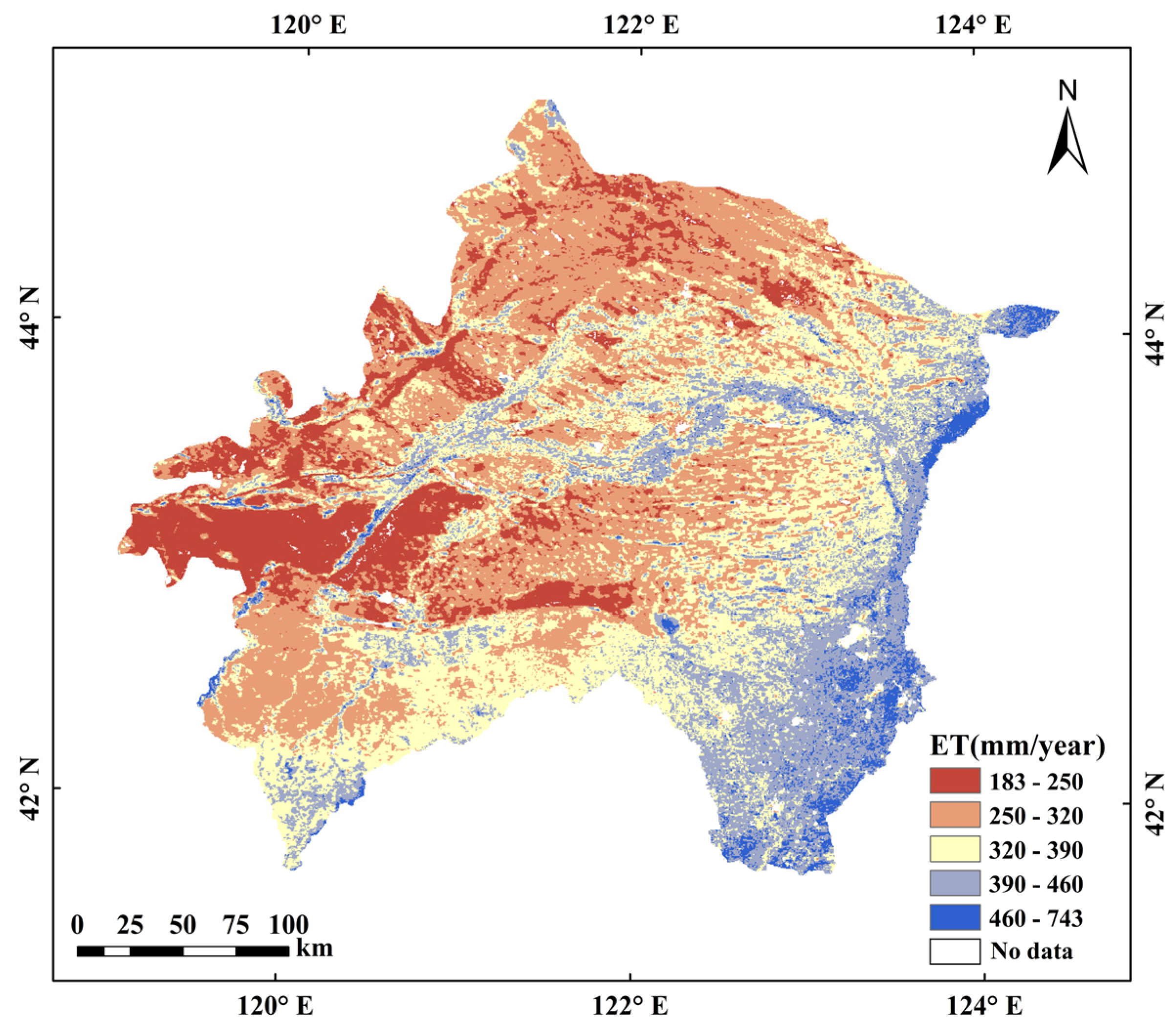
2.1. Study Area

The study area (42°18′–44°30′N, 119°14′–123°42′E) was located.0. in the south-west of the Northeast Plain of China, with a total area of about 96,000 km2 (Figure 1), consisting of the alluvial plain and residual sandy ancient alluvial plain formed by the Xiliao River and its tributaries. Hilly grassland and loess hills are the main geomorphic types in the study area. The terrain of the study area slowly inclines from west to east and presents wavy undulation, with elevation ranging from 38 m to 1200 m. The annual average temperature is 5.5 °C to 7.50 °C, sunshine hours are 2800–3100 h, and the RH is 45–58%, with a moderately temperate, semi-arid monsoon climate. The spatial and temporal distribution of PRCP is uneven; it spatially increases from northwest to southeast and is heavily concentrated in the period from June to September. The average annual precipitation is between 325 mm and 729 mm [37,52].

2.2. Data Source

2.2.1. Evapotranspiration Data

As the ET data source of the study, the MOD16 global terrestrial ET product data set acquired from the United States Geological Survey (https://earthexplorer.usgs.gov/ (accessed on 5 September 2021)) includes ET, potential evapotranspiration (PET), latent heat flux (LE), and potential latent heat flux (PLE). The data set has a spatial resolution of 500 m, and temporal resolutions are 8-day and annual syntheses [53,54]. MOD16 is based on the P-M equation to calculate wet canopy evaporation (Ewet, mm·day−1), bare soil evaporation (Es, mm·day−1), and vegetation transpiration (ET, mm·day−1) as ET (E, mm·day−1) by using remote sensing data (reflectance, vegetation coverage rate, and land cover type) and meteorological data (RH, TEMP, and air pressure) from measuring stations [25,55]. The calculation formulas are as follows:
E w e t = ( Δ × R n c + ρ × C p × f c × V P D / r h r c ) × f w e t / λ Δ + ( P a × C p × r c v ) / ( λ × ε × r h r c )
E s = [ Δ × R n s + ρ × C p × ( 1 f c ) × V P D / r a s ] / λ Δ + γ × r t o t / r a s × [ f w e t + ( 1 f w e t ) × f s m ]
E T = [ Δ × R n c + ρ × C p × ( 1 f c ) × V P D / r a ] × ( 1 f w e t ) / λ Δ + γ × ( 1 + r s ) / r a
E = E w e t + E s + E T
where ρ (kg·m−3) is the air density, Cp (MJ·kg−1·°C−1) is the specific heat capacity of air, fc is fractional vegetation cover, VPD (kPA) is the atmospheric vapor-pressure deficit, fwet is the relative surface wetness, Pa (kPA) is the atmospheric pressure, γcv (s·m−1), γhrc (s·m−1) represents the surface resistance and aerodynamic resistance to evaporated water on the wet canopy surface, ε is the ratio of the molecular weight of water to dry air (i.e., 0.622), γtot (s·m−1) is the total aerodynamic resistance, γas (s·m−1) is the aerodynamic resistance at the soil surface, fsm is the soil water constrain, γa (s·m−1), γs (s·m−1) represents the canopy surface resistance and the aerodynamic resistance between the mean canopy height and the air above the canopy, and Δ is the derivative of saturated vapor pressure to temperature [55,56].

2.2.2. Land Cover Data

Landsat remote sensing data were used to extract information regarding the spatial distribution of the various land cover types in XRP. The remote sensing data were derived from the United States Geological Survey, which contained Landsat7-ETM data from 2000 to 2013 and Landsat8-OLI data from 2014 to 2019. Images with no noise or strips and less than 5% cloud cover were selected from June to September every year. This is the period of vigorous plant growth; as such, the color and texture of the images are richer, and the characteristics of different land cover types are more obvious. Land cover types could be accurately identified according to their color, texture and other features. The selected remote sensing images were processed by ortho-correction, layer stacking, image sharpening, etc. According to the classification system of land cover data in China and the actual distribution of land cover types in the XRP, the land cover types in the study area were divided into nine categories: bare land (BAR), sand (SAN), grass (GRA), swamp (SWA), forest (FOR), cropland (CRO), paddy (PAD), water area, and construction land. According to the color, shape, texture, etc., of the remote sensing images, interpretation marks for different land cover types were established. With the support of the GIS platform, the human–machine interactive interpretation method was used to obtain the spatial distribution data of land cover types in the study area (Figure 1b).

2.2.3. Influencing Factors for Analysis Data

Wind direction speed (WDSP), PRCP, TEMP, RH, NDVI, groundwater depth, elevation, and slope were selected as factors influencing ET. Meteorological data were obtained from the China National Meteorological Information Center (http://www.nmic.cn/ (accessed on 10 September 2021)), which comprised the WDSP (m·s−1), TEMP (°C), RH (%), and PRCP (mm) of 22 meteorological stations in and around XRP from 2000 to 2019. NDVI data were derived from the MOD13 products of the United States Geological Survey. The original data were first subjected to bidirectional reflectance atmospheric correction to remove the influence of water, cloud, aerosols, and cloud shadows. The spatial resolution was 500 m, and the temporal resolution was both monthly and annual. From the Geological Cloud Information Service Platform of the China Geological Survey, data from 2019 from 138 groundwater depth monitoring stations distributed throughout the XRP and surrounding areas were used to determine groundwater depths. Elevation and slope data were derived from NASA Earthdata (https://search.earthdata.nasa.gov/ (accessed on 10 September 2021)), which provided 30 m spatial resolution DEM data covering global land.
Based on the GIS platform, the MOD16 data set was processed by ET data extraction and monthly scale data synthesis. After preprocessing by projection transformation, spatial interpolation, splicing, and clipping, the data of each influencing factor were uniformly resampled to 500 m based on the spatial resolution of the ET data. Since the MOD16 ET product used the leaf area index to indirectly reflect soil moisture content, there were no data for water and construction areas. Combined with the land cover data in the study area, we selected BAR, SAN, GRA, SWA, FOR, CRO, and PAD to analyze the temporal and spatial variation characteristics and influencing factors of ET.

2.3. Methods

2.3.1. Trend Analysis

In previous studies, scholars mostly adopted Sen’s slope to reflect the linear trends of ET changes [57]. However, without a large number of sample points, the method is easily affected by outliers. This study used Theil-Sen Median to analyze the change trends of ET in each pixel. By taking the median as the function, the Theil-Sen Median trend can reduce the impact of noise due to its insensitivity to errors and outliers [58]. The equation is as follows:
β = M e d i a n ( E T j E T i j i ) , j > i
where j and i are ordinal numbers of time, ETj and ETi represent the ET of each pixel in year j and year i, β represents the trend of change, β > 0 indicates an upward trend, and β < 0 a downward trend.

2.3.2. Significance Test

The Mann-Kendall method was used to conduct a significance analysis of the Theil-Sen trend in each pixel. This method does not require sequence data to obey normal distribution or linear trends, and it is not significantly affected by a few missing values or outliers. This method has been widely used in trend significance tests of long-term sequence data. The statistical test method is as follows: for time series ET = (ET1, ET2, …, ETn), the normalized test flux Z is defined as:
Z = { S 1 V a r ( S ) , S > 0 0 , S = 0 S + 1 V a r ( S ) , S < 0
S = i = 1 n 1 j = i + 1 n sgn ( E T j E T i )
sgn ( E T j E T i ) = { 1 , E T j E T i > 0 0 , E T j E T i = 0 1 , E T j E T i < 0
V a r ( s ) = [ n ( n 1 ) ( 2 n + 5 ) ] / 18
where n is the research period (20 years from 2000 to 2019), ETj and ETi are the values for each pixel sequence, α is defined as the significance test level, and Z(1−α)/2 is defined as a standard normal variance. When |Z| ≥ Z(1−α)/2, the null hypothesis is rejected. We set significance levels at α = 0.01, 0.05, and 0.1 [59,60].

2.3.3. Correlation Analysis

Pearson correlation coefficients (PCCs) were used to calculate the correlation coefficient between ET and various meteorological factors and NDVI in each pixel [61]. The formula is as follows:
R = i = 1 n [ ( x i x ¯ ) ( y i y ¯ ) ] i = 1 n ( x i x ¯ ) 2 [ i = 1 n ( y i y ¯ ) 2 ]
where n is the research period (i.e., from 2000 to 2019), i is the number of years, xi and yi are the values of two factors x, y in the i-year, and x ¯ , y ¯ are the n-years average of two factors.

2.3.4. Ridge Regression

Ridge regression is a biased estimation regression method for multiple collinearity data analyses. At the cost of losing part of the information or the fitting accuracy, ridge regression abandons the lack of bias of the least-square method to obtain more stable estimated results and a smaller mean square error. The ridge regression equation is as follows:
β ^ ( k ) = ( X X + k I ) 1 X y
where X′X is the coefficient matrix. When the independent variable has multiple collinearities, i.e., X′X ≈ 0 mathematically, a constant matrix kI (k > 0) is added to significantly reduce the possibility of X′X + kI being singular. Therefore, the mean square error is smaller. k is the ridge parameter whose value is not unique; theoretically, an optimal value exists. The judgment criterion was to select the minimum k as the ridge parameter when the ridge estimation of each regression coefficient was stable by observing the ridge trace graph [62]. The equation for ridge regression is as follows:
y i = β ^ 0 + β ^ 1 x 1 + β ^ 2 x 2 + + β ^ k x k
If we standardize yi and xi, then z y = y i y ¯ σ ^ y , z x j = x i j x ¯ j σ ^ j .
The normalized equation is as follows:
z ^ y = b ^ 1 z x 1 + b ^ 2 z x 2 + + b ^ k z x k
The relative contribution rate of each influencing factor to ET is calculated by Equation (14).
C h = | b ^ h | | b ^ 1 | + | b ^ 2 | + + | b ^ k |
where Ch is the relative contribution rate of a certain influencing factor to ET, and b ^ k is the regression coefficient of each influencing factor in the standardized equation. The absolute value of b ^ k represents the degree of influence of each factor on ET, and the symbol represents the positive or negative effects thereon.

3. Results

3.1. Temporal and Spatial Change of ET in the XRP

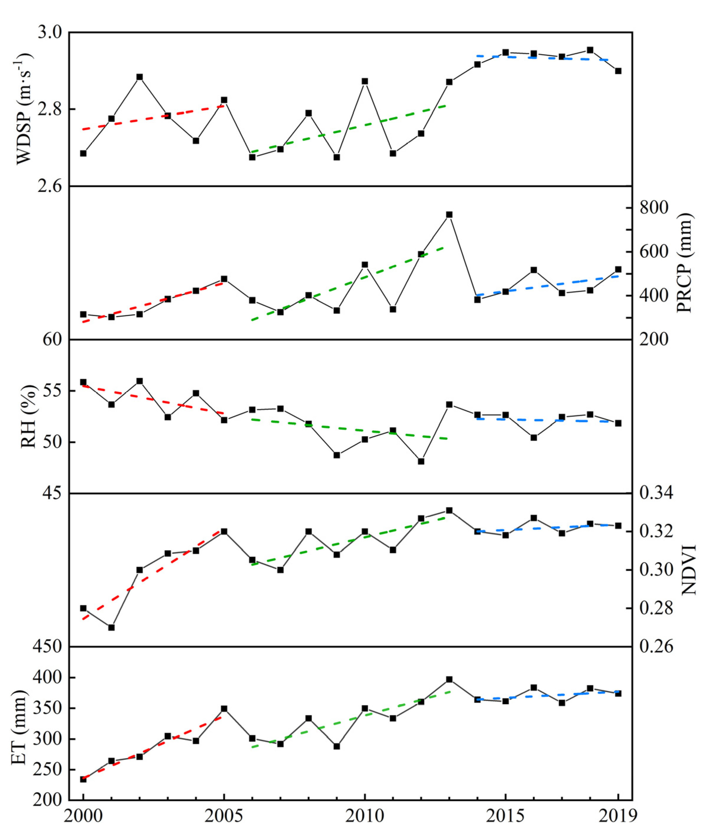
3.1.1. Interannual Change Feature

Using MOD16 ET data for XRP from 2000 to 2019, the spatial distribution characteristics of the average ET for that period were statistically analyzed. As shown in Figure 2, the spatial distribution of ET in the study area was significantly different, i.e., it was high in the east and low in the west. The mean values on a spatial scale were 183.26–743.36 mm. ET range was divided into five levels at equal intervals according to ET value distribution, and the proportion and spatial distribution of different levels were statistically analyzed. The low-value areas of ET (183–250 mm) accounted for 13.68% of the total area; these were mostly concentrated in the central and western regions of the study area. The high-value areas (460–743 mm) accounted for only 3.27% of the total area, and were mostly concentrated in the southeast of the study area.
To study the temporal variation characteristics of ET in different land cover types, we combined ET with data regarding land cover types to statistically analyze the interannual variation trends of ET in BAR, SAN, GRA, SWA, FOR, CRO, and PAD from 2000 to 2019 (Figure 3). Among the seven land cover types, the annual average ET varied significantly. In PAD it was the largest (421.15 mm), followed by CRO (344.22 mm), FOR (332.84 mm), SWA (278.89 mm), GRA (271.89 mm), and SAN (246.80 mm). The annual average of ET was the lowest in BAR, i.e., only 240.58 mm. The temporal variation characteristics of ET in different land cover types were relatively consistent, showing an overall increasing trend. The peak value appeared in 2013. Among different land cover types, the increasing trend in CRO was the most significant, with a growth rate of 7.60 mm/year, and least significant in BAR, with the growth rate of 4.79 mm/year.
In order to study spatial variation, we analyzed the trend of ET by Theil-Sen Median based on MOD16 ET data from 2000 to 2019 in the XRP, and used the Mann-Kendall trend to test the significance of the observed trends. α was defined as the level of a significance test; α = 0.1, 0.05, 0.01 corresponded to |Z| ≥ 1.645, 1.96, 2.576, respectively, indicating that the study sequence passed a 90%, 95%, and 99% reliability of significance test, respectively. |Z| ≤ 1.645 indicated that the study sequence did not pass the significance test with a reliability of 90%. Regarding spatial distribution from 2000 to 2019 (Figure 4), ET showed an increasing trend in 99.42% of the study area. Only 0.58% of the area showed a decreasing trend; this was concentrated in the central and southeast of the study area. Notably, 93.67% of the area showed an increasing trend that surpassed α = 0.01 significance.

3.1.2. Monthly Change Characteristics

Our statistical analysis of monthly ET distribution in the study area was based on MOD16 ET data from 2000 to 2019 (Figure 5). The monthly mean of ET ranged from 5.8 mm to 148.88 mm, and the spatial distribution had obvious temporal differences. The monthly ET decreased from south to north in January, February, and December. From March to November, the it showed strong distribution in the southeast and low distribution in the northwest. The spatial distribution difference from June to September was particularly obvious. The highest monthly ET that appeared in the southeast of the study area in July was 135.04 mm higher than the lowest monthly ET, which was observed in the north of the study area in the same period.
The monthly ET trends of different land cover types from 2000 to 2019 in the XRP were analyzed. Figure 6 shows a single peak change of ET for all land cover types, as well as a peak appearing in July and August. By comparing the monthly ET, we found that the ET differences between different land cover types in the study area mainly occurred in July and August. The monthly ET of PAD was the highest (94.81 mm) in July, i.e., 59.29 mm higher than that of BAR, the lowest in the same period. Except for July and August, there was no significant difference in the monthly ET between different land cover types in the same month.

3.2. Correlation Analysis of ET Influencing Factors

3.2.1. Correlation with Meteorological Factors

As an important environmental factor, meteorological elements are irreplaceable in all aspects of the ecosystem. WDSP, TEMP, RH, and PRCP are important meteorological factors affecting the inland water cycle [38,63]. In order to explore the influence of meteorological factors on ET, the PCCs between annual ET and WDSP, RH, TEMP, PRCP were calculated using MOD16 ET data and annual raster data regarding meteorological factors in the XRP based on the GIS platform (Figure 7). The spatial distribution of PCCs between ET and WDSP was significantly different. The areas with significant positive correlation (PCCs > 0.7), concentrated in the central and southeast of the study area, accounted for 31.06% of the total. By contrast, in the west of the study area, 15.68% of the total showed negative correlation. ET and RH were mainly negatively correlated, and the correspondent areas with significant negative correlation (PCCs < −0.7) accounted for 12.71% of the study area; these were concentrated in the central and northern areas. The absolute value of the PCCs between ET and TEMP was less than 0.5, showing a weak correlation. The positively correlated areas accounted for 41.64%; these were mainly concentrated in the northwest and east of the study area. ET and PRCP were positively correlated in the study area, i.e., more significantly in the northwest than in the southeast. The areas with significant positive correlation (PCCs > 0.7) accounted for 54.48% of the study area.
In order to study the correlation between ET and meteorological factors for different land cover types, the PCCs between the two elements were calculated (Figure 8). The results revealed that the PCCs between ET and WDSP in GRA, CRO, PAD, SWA ranged from 0.06 to 0.97, showing a relatively strong positive correlation. Among them, the positive correlation of PAD was the most significant, with an average PCC of 0.67. However, ET and WDSP showed a negative correlation in more than 75% of BAR areas. The PCCs between ET and RH were negative in GRA, CRO, and SWA, indicating a strong negative correlation. The negative correlation of GRA was the most obvious, with an average PCC of −0.52. The absolute values of the average PCCs between ET and TEMP in all land cover types were less than 0.2, showing no correlation. ET and PRCP showed a significant positive correlation in all land cover types. Except for PAD, the average PCCs between ET and PRCP were above 0.7.

3.2.2. Correlation with NDVI

Vegetation transpiration is the main mechanism of ET. It is mainly affected by vegetation species, root depth, and plant moisture content, and varies with vegetation growth and coverage. NDVI is the best indicator of growth status and spatial distribution density of vegetation. It is linearly correlated with vegetation distribution density and can effectively reflect the growth status [64,65]. In order to explore the influence of vegetation growth status and coverage on ET, the PCCs between annual ET and NDVI were calculated based on the GIS platform in each pixel. As shown in Figure 9, ET and NDVI were mainly positively correlated in the study area, with an average of 0.71. The areas with significant positive correlation (PCCs > 0.7) account for 76.34% of the study area. The areas with weak correlation (−0.5 < PCCs < 0.5) account for 12.14%, and were mainly concentrated in the south-east and middle-west of the study area. Based on the land cover data of XRP, the PCCs between ET and NDVI in different land cover types were statistically analyzed. As shown in Figure 10, the positive correlation between ET and NDVI was significant in CRO and FOR with higher vegetation density. The PCCs of more than 75% of the areas were over 0.6; the FOR average was the largest, i.e., up to 0.81. However, in BAR and SAN, with lower vegetation density, the average PCCs between ET and NDVI were only about 0.3, showing a relatively weak correlation. In GRA, PAD, and SWA, though the PCCs between ET and NDVI had a wide range, the average values were more than 0.6.

3.2.3. Correlation with Groundwater Depth

ET can be divided into soil moisture evaporation and groundwater evaporation from evaporated water sources. Groundwater evaporation is the process in which groundwater is transported to the gas belt and the atmosphere through soil evaporation and plant transpiration. It is the main mechanism for the transformation of groundwater to soil moisture and atmospheric water [66]; its extent is mainly affected by groundwater depth. According to the situation in the XRP, the groundwater depth was divided into 14 levels at intervals of 1 m. As shown in Figure 11a, the groundwater depths in the study area ranged from 1.14 m to 14.89 m, and were generally deeper in the west and shallower in the east. The areas with groundwater depths of over 6.0 m were mainly concentrated in the northwest and middle-west of the study area. A spatial overlay analysis of ET, land cover types, and groundwater depth data was carried out to calculate the mean ET corresponding to the different groundwater depths in each land cover type. Figure 11b illustrates that ET decreases significantly with the increase in groundwater depth in GRA, CRO, BRA, SAN, and SWA. In FOR and PAD, although ET also decreased with the increase of groundwater depth, the curves had significantly greater fluctuation, indicating the minor effect of groundwater depth on ET in FOR and PAD. In SWA, GRA, and CRO, the influence of groundwater depth on ET was relatively consistent. When the groundwater depth was less than 3.0 m, the curves had no obvious change trend, indicating that the evaporated water in the surface soil could be fully replenished by groundwater through capillary action. Therefore, ET was not affected by groundwater depth. When the groundwater depth was more than 3.0 m, the curves showed a downward trend with the increase of groundwater depth, indicating that with the increase of water transport distance, the water supplied to the surface by capillary action, was reduced, thereby also decreasing ET. When the groundwater depth was 6.0 m, ET was lowest and tended to be stable. Meanwhile, ET was mainly dominated by soil moisture evaporation and vegetation transpiration. Therefore, the limit depths of groundwater evaporation of SWA, GRA, and CRO in the XRP could be determined as 6.0 m. In BAR and SAN, ET also decreased with the increase of groundwater depth and remained steady when the depth reached 4.0 m, indicating that the limit depth of groundwater evaporation in BAR and SAN in the XRP was 4.0 m. These findings imply that vegetation can increase the depth of the groundwater absorbed by land due to the water potential difference caused by transpiration allowing plant roots to absorb water.

3.2.4. Correlation with Topography Factors

Elevation and slope are basic topographical characteristics and the main factors affecting species, growth states, and the spatial distribution of vegetation. Their change alters soil moisture and surface runoff, thereby influencing ET. An elevation distribution map of XRP was made using ASTER DEM data. According to their distribution characteristics, the elevations were divided into 10 categories (0–100 m, 100–200 m, 200–300 m, 300–400 m, 400–500 m, 500–600 m, 600–700 m, 700–800 m, 800–900 m, and 900–1000 m). As shown in Figure 12a, the geography of the XRP is low and flat, tilting from the southwest to the northeast, with an average elevation of 253.94 m above sea level. A spatial overlay analysis of ET, land cover types, and elevation data in the study area was carried out to calculate the mean ET corresponding to different elevation levels for each land cover type. As shown in Figure 12b, except for PAD, the elevation effects on ET were relatively consistent. ET decreased obviously with the increase of elevation and tended to be stable when the elevation reached 300 m, indicating that elevation has a negative influence on ET when below 300 m. Although the ET of PAD showed a decreasing trend with the increase of elevation, the fluctuations in the curve indicate only slight effects. These phenomena may be related to surface runoff. After rainfall, rainwater is more likely to collect at low altitude areas, providing more water sources for ET. Affected by artificial irrigation, PAD has sufficient water, so it is not affected.
Based on ASTER DEM data, a slope distribution map of the XRP (Figure 13a) was made. According to the classification standard of landform slopes by the International Geographical Union, the slope of the XRP was divided into six categories (0–0.5°, 0.5–2°, 2–5°, 5–15°, 15–35°, and 35–55°). The average ET of the different slope levels for each land cover type was calculated. As shown in Figure 13b, except for PAD, the slope effects on ET were relatively consistent. When the slope was less than 15°, ET changed slightly, and remained stable with the increase of slope. When the slope was greater than 15°, ET increased obviously with the increase of slope. This may have been caused by the relatively fast flow rate of rainwater in areas with large slopes. The larger the slope, the faster the runoff, and thus, the greater the ET. However, due to the low adhesion and loose texture of sand, SAN had a strong absorption capacity for rainwater, preventing it from forming surface runoff, even in areas with large slopes. Therefore, slope had no significant effect on ET in SAN. This implies that the influence of topographic conditions on ET may be mainly reflected in the differences in water conditions caused by surface runoff.

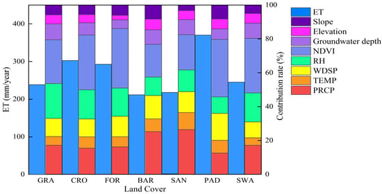
3.3. The Relative Contribution Rate of Influencing Factors to ET

ET and its influencing factors showed different correlations for different land cover types. In this study, we used the raster data of annual average ET (mm), WDSP (m·s−1), TEMP (°C), PRCP (mm), RH (%), NDVI, groundwater depth (m), meters above sea level (m), and slope (°) in the study area from 2000 to 2019 to create a multisource spatial data set. Using this, we conducted spatial balance sampling in different land cover types at 5-km intervals. Then, we took the WDSP, TEMP, PRCP, RH, NDVI, groundwater depth, elevation, and slope as the inputs (Xi) for the training sample and the annual ET value as the output (Yi) to construct a training sample set (Xi, Yi) in order to construct the statistical regression analysis model to quantitatively analyze the influence of various factors on ET. Independent variables showed multicollinearity because of their correlations. Linear regression can lead to overfitting of the regression equation, causing the independent variable coefficient to fail to conform to the actual meaning of the influencing factors. Therefore, it was necessary to diagnose the collinearity of each influencing factor before constructing the regression model. The variance inflation factor (VIF) was generally used as the standard of collinearity diagnoses. If VIF was greater than 10, it indicated that the model had serious multicollinearity. The collinearity diagnostic results (Figure 14a) showed that the VIFs of PRCP, RH and, NDVI were greater than 10, indicating significant multicollinearity. In order to weaken the influence of multicollinearity in independent variables on the regression coefficient of the model, this study used ridge regression analysis to achieve a more realistic regression result at the expense of rejecting some information and reducing the accuracy of the model [62].
From the results of our ridge regression analysis (Figure 14b, Table 1), the multicollinearity among the influencing factors was shown to be significantly weakened (VIF < 10), and the model determination coefficient (R2) reached more than 0.6 for all land cover types. PRCP, NDVI, and slope had positive effects on ET for all land cover types, while RH, groundwater depth, and elevation had negative effects. It is noteworthy that TEMP had a negative effect on ET in GRA, BAR, and SAN, while WDSP had a negative effect on ET in BAR and SAN, and TEMP and WDSP had a positive effect on ET in other land cover types.
We calculated the relative contribution rate of each influencing factor to ET in different land cover types according to the ridge regression analysis results. In Figure 15, the NDVI, RH, PRCP, and WDSP represent a cumulative contribution rate of over 60% to ET in all land cover types, thereby serving as the main influencing factors. The NDVI, RH, PRCP, WDSP, and groundwater depth in GRA, CRO, and SWA represent a cumulative contribution rate of over 80%, comprising the best explanation for changes in ET. In FOR, NDVI shows the largest relative contribution rate, i.e., 35.09%, making it the largest affecting factor, followed by RH, PRCP, WDSP, slope, and groundwater depth. NDVI is also the leading determinant of ET in PAD, although the influence of WDSP is greater than that of PRCP and RH. In BAR and SAN, PRCP is the leading determinant of ET, followed by NDVI, WDSP, and RH.

4. Discussion

4.1. Reason Analysis of Temporal Changes in ET

This study found that among the various factors, NDVI, RH, PRCP, and WDSP were the leading determinants of interannual ET changes for all land cover types. Through a comparative analysis of the interannual trends of ET, NDVI, RH, PRCP, and WDSP in the XRP from 2000 to 2019 (Figure 16), ET changes were divided into three periods: the first was a rising period from 2000 to 2005, the second another rising period from 2006 to 2013, and the third a stable period from 2014 to 2019. The first period represented the most significant ET increase, with a 7.06% average growth rate. During this period, only RH showed a decreasing trend, while NDVI, WDSP, and PRCP increased. These changes benefited the increase of ET. The increase of NDVI was the most significant, with an average annual growth rate of 3.57%; this may have been the main reason for the increase in ET. In the second period, ET showed a relatively smooth increase, with an average growth rate of 3.86%. NDVI represented a relatively smooth increasing trend, while RH basically showed a consistent increase relative to the previous period. The significant increase of PRCP and WDSP may have been the main driving forces of ET increase during this period. In 2014–2019, NDVI, RH, PRCP, and WDSP tended to be stable, and the annual average ET remained unchanged at about 370 mm. The results showed that the change of climatic factors had a significant influence on ET, consistent with results for most basins in China, such as the Pearl River and Tao River Basins. However, the difference lay in the fact that TEMP is the main climatic factor affecting ET in the aforementioned basins [43,67]. In this study, RH, PRCP, and WDSP were found to have a large influence on ET. This may have been related to climate variability and the distribution of water resources in different regions [68,69,70,71]. Combined with the results of this study, TEMP and other energy conditions are the main drivers for ET change in humid or subhumid climate areas where water resources are relatively abundant. In contrast, in arid climates with relatively scarce water resources, water conditions such as vegetation and PRCP can further determine changes in ET. This further explains why changes in ET are subject to multiple influencing factors, and why the main factors vary in different periods or under different climatic conditions [41,42,43,44,72].

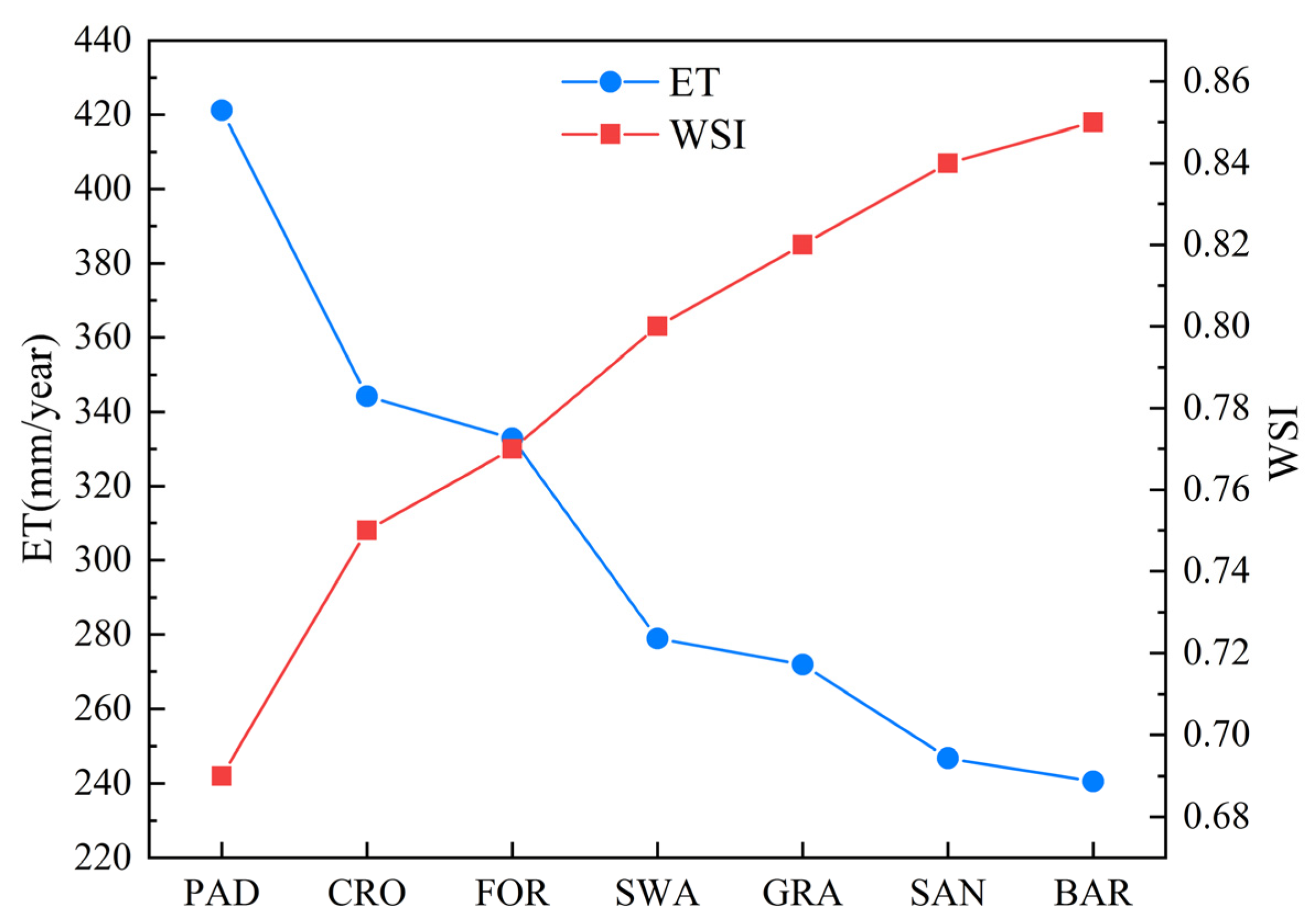
4.2. Analysis of ET Differences for Different Land Cover Types

The factors affecting ET can be divided into three categories: water conditions, energy conditions, and dynamic conditions. The water conditions describe the amount of water output on the evaporation surface. The energy conditions indicate the speed of water conversion from liquid to gas, and the dynamic conditions indicate the speed of water vapor transport over the evaporation surface. As the main parameter to reflect pressure on water resources, the water stress index (WSI) is closely related to water resource quantity [73]. In order to further explore the reasons behind the obvious differences in ET, we used WSI to analyze the influence of water conditions on ET for different land cover types. As shown in Figure 17, the WSI for different land cover types varied significantly; notably, ET decreased with the increase of WSI. In PAD and CRO, artificial irrigation ensures sufficient water resources, i.e., a smaller WSI corresponds to greater ET. For other land cover types, PRCP and capillary action (which transports groundwater to the surface) were the main sources of surface water. Meanwhile, different species and densities of vegetation were key factors influencing the absorption of groundwater and the maintenance of the water content in surface soil. The ultimate depths after absorbing groundwater in FOR, SWA, and GRA were greater than those of SAN and BAR. The groundwater transported more water to the surface through capillary action. Moreover, the vegetation coverage of FOR, SWA, and GRA was greater. The interception of canopies and leaves during rainfall lessens rainwater infiltration and increases the surface soil moisture content. Therefore, the WSI of FOR, SWA, and GRA was smaller than that of SAN and BAR; as such, the former three types demonstrated greater ET. This indicated that the water conditions in high-latitude, arid areas significantly affects ET in various land cover types. The difference of ET among different land covers was not only due to the different water conditions, but also to the different mechanisms of action and degrees of the energy conditions and dynamic conditions required for evaporation in different land covers. TEMP, as the main energy condition, showed a different correlation with ET in different land covers. An increase of TEMP not only accelerated water evaporation in the soil, but also controlled the stomatal opening of plants, resulting in changes of vegetation evapotranspiration. This indicated that the influence of TEMP on ET was different in areas with different vegetation coverage. As the main dynamic conditions, the effects of RH and WDSP on ET were obviously different for different land covers. Only in SAN and BAR soil with serious water stress did WDSP have a negative effect. This may be because in areas with low water stress, WDSP accelerates the rising speed of water vapor above the evaporation surface, thus accelerating the rate of ET, while in SAN and BAR (without vegetation cover), the surface is gradually weathered, resulting in a negative impact. Therefore, studying the temporal and spatial changes of ET and its influencing factors from the perspective of the water cycle characteristics of different land cover types is necessary for understanding variability in the hydrologic cycle.
W S I = 1 E T P E T

5. Conclusions

The differences among water evaporation mechanisms and action conditions in different land cover types result in varying ET for different land cover types. These differences are reflected not only in the changing trends, but also in the main factors influencing ET. We analyzed the spatiotemporal variation of ET for different land cover types and its correlations with meteorological factors, NDVI, groundwater depth, elevation, and slope, and applied the ridge regression model to quantify the contributions of these factors. In the past 20 years, due to vegetation greening and increasing precipitation, ET showed an increasing trend at a rate of 6.72 mm/year. This trend was most obvious in CRO, resulting in additional pressure on agricultural irrigation. Therefore, we should pay more attention to the soil moisture content in CRO and carry out agricultural irrigation in a timely manner, in order to ensure that appropriate amounts of water are being delivered for crop growth. Although the correlations among ET and the aforementioned factors were quite different for different land cover types, NDVI, RH, PRCP, and WDSP were shown to have a cumulative contribution rate of more than 60% in all land cover types, and could serve as the main determinants of ET. In GRA, CRO, PAD, FOR and SWA, NDVI had the greatest influence, while PRCP was the dominant influencing factor for BAR and SAN. Therefore, policymakers should apply targeted measures for water resources management for different land cover types. Especially in SAN and BAR with severe water stress, afforestation should be increased to maintain soil water availability. Although there were some limitations in this study, i.e., the differences of ecological and climatic environments in different regions, our results emphasize the importance of comprehensively considering the differences among various hydrologic cycles according to land cover type to assess the contributions of influencing factors to ET. In the future, we will conduct further research on the hydrologic cycle in humid and semihumid regions.

Author Contributions

Conceptualization, N.L. and R.J.; methodology, Q.L.; validation, H.Y.; investigation H.L. and Q.Y.; writing—original draft preparation, N.L. and R.J.; writing—review and editing, N.L. and R.J. All authors have read and agreed to the published version of the manuscript.

Funding

The research was sponsored by National Natural Science Foundation of China (41702357 and 41801283) and Geological Survey project of China Geological Survey (DD20190340).

Acknowledgments

The authors would like to thank the United States Geological Survey for providing MODIS, and Landsat data. The anonymous reviewers to improve the quality of this manuscript are greatly appreciated.

Conflicts of Interest

The authors declare no conflict of interest.

References

  1. Jung, M.; Reichstein, M.; Ciais, P.; Seneviratne, S.I.; Sheffield, J.; Goulden, M.L.; Bonan, G.; Cescatti, A.; Chen, J.; de Jeu, R.; et al. Recent decline in the global land evapotranspiration trend due to limited moisture supply. Nature 2010, 467, 951–954. [Google Scholar] [CrossRef]
  2. Anderson, M.C.; Norman, J.M.; Mecikalski, J.R.; Otkin, J.A.; Kustas, W.P. A climatological study of evapotranspiration and moisture stress across the continental United States based on thermal remote sensing: 2. Surface moisture climatology. J. Geophys. Res. Atmos. 2007, 112, D11112. [Google Scholar] [CrossRef]
  3. Allen, R.G.; Pereira, L.S.; Howell, T.A.; Jensen, M.E. Evapotranspiration information reporting: I. Factors governing measurement accuracy. Agric. Water Manag. 2011, 98, 899–920. [Google Scholar] [CrossRef] [Green Version]
  4. Bisquert, M.; Sanchez, J.M.; Lopez-Urrea, R.; Caselles, V. Estimating high resolution evapotranspiration from disaggregated thermal images. Remote Sens. Environ. 2016, 187, 423–433. [Google Scholar] [CrossRef]
  5. Ma, Q.; Zhang, J.; Sun, C.; Guo, E.; Zhang, F.; Wang, M. Changes of Reference Evapotranspiration and Its Relationship to Dry/Wet Conditions Based on the Aridity Index in the Songnen Grassland, Northeast China. Water 2017, 9, 316. [Google Scholar] [CrossRef] [Green Version]
  6. Guo, D.; Westra, S.; Maier, H.R. Sensitivity of potential evapotranspiration to changes in climate variables for different Australian climatic zones. Earth Syst. Sci. 2017, 21, 2107–2126. [Google Scholar] [CrossRef] [Green Version]
  7. Espadafor, M.; Lorite, I.J.; Gavilan, P.; Berengena, J. An analysis of the tendency of reference evapotranspiration estimates and other climate variables during the last 45 years in Southern Spain. Agric. Water Manag. 2011, 98, 1045–1061. [Google Scholar] [CrossRef]
  8. Tabari, H.; Marofi, S.; Aeini, A.; Talaee, P.H.; Mohammadi, K. Trend analysis of reference evapotranspiration in the western half of Iran. Agric. For. Meteorol. 2011, 151, 128–136. [Google Scholar] [CrossRef]
  9. French, A.N.; Hunsaker, D.J.; Thorp, K.R. Remote sensing of evapotranspiration over cotton using the TSEB and METRIC energy balance models. Remote Sens. Environ. 2015, 158, 281–294. [Google Scholar] [CrossRef]
  10. Thomas, A. Spatial and temporal characteristics of potential evapotranspiration trends over China. Int. J. Climatol. 2000, 20, 381–396. [Google Scholar] [CrossRef]
  11. Doll, P. Impact of climate change and variability on irrigation requirements: A global perspective. Clim. Chang. 2002, 54, 269–293. [Google Scholar] [CrossRef]
  12. Parmesan, C.; Yohe, G. A globally coherent fingerprint of climate change impacts across natural systems. Nature 2003, 421, 37–42. [Google Scholar] [CrossRef] [PubMed]
  13. Pritchard, H.D. Asia’s shrinking glaciers protect large populations from drought stress. Nature 2019, 569, 649–654. [Google Scholar] [CrossRef] [PubMed]
  14. Walther, G.R.; Post, E.; Convey, P.; Menzel, A.; Parmesan, C.; Beebee, T.J.C.; Fromentin, J.M.; Hoegh-Guldberg, O.; Bairlein, F. Ecological responses to recent climate change. Nature 2002, 416, 389–395. [Google Scholar] [CrossRef] [PubMed]
  15. Williamson, C.E.; Saros, J.E.; Schindler, D.W. CLIMATE CHANGE Sentinels of Change. Science 2009, 323, 887–888. [Google Scholar] [CrossRef] [PubMed]
  16. Choi, M.; Kustas, W.P.; Anderson, M.C.; Allen, R.G.; Li, F.; Kjaersgaard, J.H. An intercomparison of three remote sensing-based surface energy balance algorithms over a corn and soybean production region (Iowa, US) during SMACEX. Agric. For. Meteorol. 2009, 149, 2082–2097. [Google Scholar] [CrossRef]
  17. Ershadi, A.; McCabe, M.F.; Evans, J.P.; Walker, J.P. Effects of spatial aggregation on the multi-scale estimation of evapotranspiration. Remote Sens. Environ. 2013, 131, 51–62. [Google Scholar] [CrossRef]
  18. Bindhu, V.M.; Narasimhan, B.; Sudheer, K.P. Development and verification of a non-linear disaggregation method (NL-DisTrad) to downscale MODIS land surface temperature to the spatial scale of Landsat thermal data to estimate evapotranspiration. Remote Sens. Environ. 2013, 135, 118–129. [Google Scholar] [CrossRef]
  19. Mahmoud, S.H.; Alazba, A.A. A coupled remote sensing and the Surface Energy Balance based algorithms to estimate actual evapotranspiration over the western and southern regions of Saudi Arabia. J. Asian Earth Sci. 2016, 124, 269–283. [Google Scholar] [CrossRef]
  20. Allies, A.; Demarty, J.; Olioso, A.; Moussa, I.B.; Issoufou, H.B.A.; Velluet, C.; Bahir, M.; Mainassara, I.; Oi, M.; Chazarin, J.P.; et al. Evapotranspiration Estimation in the Sahel Using a New Ensemble-Contextual Method. Remote Sens. 2020, 12, 34. [Google Scholar] [CrossRef] [Green Version]
  21. Costa, J.D.; Jose, J.V.; Wolff, W.; de Oliveira, N.P.R.; Oliveira, R.C.; Ribeiro, N.L.; Coelho, R.D.; da Silva, T.J.A.; Bonfim-Silva, E.M.; Schlichting, A.F. Spatial variability quantification of maize water consumption based on Google EEflux tool. Agric. Water Manag. 2020, 232, 8. [Google Scholar] [CrossRef]
  22. Ahmed, K.R.; Paul-Limoges, E.; Rascher, U.; Damm, A. A First Assessment of the 2018 European Drought Impact on Ecosystem Evapotranspiration. Remote Sens. 2021, 13, 16. [Google Scholar] [CrossRef]
  23. Ghiat, I.; Mackey, H.R.; Al-Ansari, T. A Review of Evapotranspiration Measurement Models, Techniques and Methods for Open and Closed Agricultural Field Applications. Water 2021, 13, 19. [Google Scholar] [CrossRef]
  24. Sirisena, T.A.J.G.; Maskey, S.; Ranasinghe, R. Hydrological Model Calibration with Streamflow and Remote Sensing Based Evapotranspiration Data in a Data Poor Basin. Remote Sens. 2020, 12, 3768. [Google Scholar] [CrossRef]
  25. Penman, H.L. Natural evaporation from open water, hare soil and grass. Proc. R. Soc. Lond. 1948, 193, 120–145. [Google Scholar] [CrossRef] [Green Version]
  26. Ershadi, A.; McCabe, M.F.; Evans, J.P.; Wood, E.F. Impact of model structure and parameterization on Penman-Monteith type evaporation models. J. Hydrol. 2015, 525, 521–535. [Google Scholar] [CrossRef] [Green Version]
  27. Long, D.; Longuevergne, L.; Scanlon, B.R. Uncertainty in evapotranspiration from land surface modeling, remote sensing, and GRACE satellites. Water Resour. Res. 2014, 50, 1131–1151. [Google Scholar] [CrossRef] [Green Version]
  28. Ramoelo, A.; Majozi, N.; Mathieu, R.; Jovanovic, N.; Nickless, A.; Dzikiti, S. Validation of Global Evapotranspiration Product (MOD16) using Flux Tower Data in the African Savanna, South Africa. Remote Sens. 2014, 6, 7406–7423. [Google Scholar] [CrossRef] [Green Version]
  29. Corbari, C.; Jovanovic, D.S.; Nardella, L.; Sobrino, J.; Mancini, M. Evapotranspiration Estimates at High Spatial and Temporal Resolutions from an Energy-Water Balance Model and Satellite Data in the Capitanata Irrigation Consortium. Remote Sens. 2020, 12, 4083. [Google Scholar] [CrossRef]
  30. Fisher, J.B.; Lee, B.; Purdy, A.J.; Halverson, G.H.; Dohlen, M.B.; Cawse-Nicholson, K.; Wang, A.; Anderson, R.G.; Aragon, B.; Arain, M.A.; et al. ECOSTRESS: NASA’s Next Generation Mission to Measure Evapotranspiration from the International Space Station. Water Resour. Res. 2020, 56, e2019WR026058. [Google Scholar] [CrossRef]
  31. Xiao, Z.; Liang, S.; Wang, J.; Xiang, Y.; Zhao, X.; Song, J. Long-Time-Series Global Land Surface Satellite Leaf Area Index Product Derived from MODIS and AVHRR Surface Reflectance. IEEE Trans. Geosci. Remote Sens. 2016, 54, 5301–5318. [Google Scholar] [CrossRef]
  32. Zhu, G.; Zhang, K.; Chen, H.; Wang, Y.; Su, Y.; Zhang, Y.; Ma, J. Development and evaluation of a simple hydrologically based model for terrestrial evapotranspiration simulations. J. Hydrol. 2019, 577, 123928. [Google Scholar] [CrossRef]
  33. Pascolini-Campbell, M.; Reager, J.T.; Chandanpurkar, H.A.; Rodell, M. A 10 per cent increase in global land evapotranspiration from 2003 to 2019. Nature 2021, 593, 543–547. [Google Scholar] [CrossRef] [PubMed]
  34. Yang, Z.; Zhang, Q.; Hao, X.; Yue, P. Changes in Evapotranspiration Over Global Semiarid Regions 1984–2013. J. Geophys. Res. Atmos. 2019, 124, 2946–2963. [Google Scholar] [CrossRef]
  35. Nagler, P.L.; Barreto-Munoz, A.; Borujeni, S.C.; Nouri, H.; Jarchow, C.J.; Didan, K. Riparian Area Changes in Greenness and Water Use on the Lower Colorado River in the USA from 2000 to 2020. Remote Sens. 2021, 13, 1332. [Google Scholar] [CrossRef]
  36. Rigden, A.J.; Salvucci, G.D. Stomatal response to humidity and CO2 implicated in recent decline in US evaporation. Glob. Change Biol. 2017, 23, 1140–1151. [Google Scholar] [CrossRef]
  37. Gao, Z.; He, J.; Dong, K.; Bian, X.; Li, X. Sensitivity study of reference crop evapotranspiration during growing season in the West Liao River basin, China. Theor. Appl. Climatol. 2016, 124, 865–881. [Google Scholar] [CrossRef]
  38. Wang, Z.; Xie, P.; Lai, C.; Chen, X.; Wu, X.; Zeng, Z.; Li, J. Spatiotemporal variability of reference evapotranspiration and contributing climatic factors in China during 1961–2013. J. Hydrol. 2017, 544, 97–108. [Google Scholar] [CrossRef]
  39. Zhang, B.; Xu, D.; Liu, Y.; Li, F.; Cai, J.; Du, L. Multi-scale evapotranspiration of summer maize and the controlling meteorological factors in north China. Agric. For. Meteorol. 2016, 216, 1–12. [Google Scholar] [CrossRef]
  40. Javadian, M.; Behrangi, A.; Smith, W.K.; Fisher, J.B. Global Trends in Evapotranspiration Dominated by Increases across Large Cropland Regions. Remote Sens. 2020, 12, 1221. [Google Scholar] [CrossRef] [Green Version]
  41. Nooni, I.K.; Wang, G.; Hagan, D.F.T.; Lu, J.; Ullah, W.; Li, S. Evapotranspiration and its Components in the Nile River Basin Based on Long-Term Satellite Assimilation Product. Water 2019, 11, 1400. [Google Scholar] [CrossRef] [Green Version]
  42. Yang, Z.; Zhang, Q.; Hao, X. Evapotranspiration Trend and Its Relationship with Precipitation over the Loess Plateau during the Last Three Decades. Adv. Meteorol. 2016, 2016, 6809749. [Google Scholar] [CrossRef] [Green Version]
  43. Zhang, T.; Chen, Y. Analysis of Dynamic Spatiotemporal Changes in Actual Evapotranspiration and Its Associated Factors in the Pearl River Basin Based on MOD16. Water 2017, 9, 832. [Google Scholar] [CrossRef] [Green Version]
  44. Zhang, L.; Yao, Y.; Wang, Z.; Jia, K.; Zhang, X.; Zhang, Y.; Wang, X.; Xu, J.; Chen, X. Satellite-Derived Spatiotemporal Variations in Evapotranspiration over Northeast China during 1982–2010. Remote Sens. 2017, 9, 1140. [Google Scholar] [CrossRef] [Green Version]
  45. Chu, R.; Li, M.; Islam, A.R.M.T.; Fei, D.; Shen, S. Attribution analysis of actual and potential evapotranspiration changes based on the complementary relationship theory in the Huai River basin of eastern China. Int. J. Climatol. 2019, 39, 4072–4090. [Google Scholar] [CrossRef]
  46. Wang, Z.; Ye, A.; Wang, L.; Liu, K.; Cheng, L. Spatial and temporal characteristics of reference evapotranspiration and its climatic driving factors over China from 1979–2015. Agric. Water Manag. 2019, 213, 1096–1108. [Google Scholar] [CrossRef]
  47. Valipour, M.; Bateni, S.M.; Gholami Sefidkouhi, M.A.; Raeini-Sarjaz, M.; Singh, V.P. Complexity of Forces Driving Trend of Reference Evapotranspiration and Signals of Climate Change. Atmosphere 2020, 11, 1081. [Google Scholar] [CrossRef]
  48. Jerin, J.N.; Islam, H.M.T.; Islam, A.R.M.T.; Shahid, S.; Hu, Z.; Badhan, M.A.; Chu, R.; Elbeltagi, A. Spatiotemporal trends in reference evapotranspiration and its driving factors in Bangladesh. Theor. Appl. Climatol. 2021, 144, 793–808. [Google Scholar] [CrossRef]
  49. Qiu, R.; Katul, G.G.; Wang, J.; Xu, J.; Kang, S.; Liu, C.; Zhang, B.; Li, L.; Cajucom, E.P. Differential response of rice evapotranspiration to varying patterns of warming. Agric. For. Meteorol. 2021, 298, 108293. [Google Scholar] [CrossRef]
  50. Sterling, S.M.; Ducharne, A.; Polcher, J. The impact of global land-cover change on the terrestrial water cycle. Nat. Clim. Change 2013, 3, 385–390. [Google Scholar] [CrossRef]
  51. Jin, X.; Chen, M.; Fan, Y.; Yan, L.; Wang, F. Effects of Mulched Drip Irrigation on Soil Moisture and Groundwater Recharge in the Xiliao River Plain, China. Water 2018, 10, 1755. [Google Scholar] [CrossRef] [Green Version]
  52. Zhu, L.; Gong, H.; Dai, Z.; Xu, T.; Su, X. An integrated assessment of the impact of precipitation and groundwater on vegetation growth in arid and semiarid areas. Environ. Earth Sci. 2015, 74, 5009–5021. [Google Scholar] [CrossRef] [Green Version]
  53. Mu, Q.; Heinsch, F.A.; Zhao, M.; Running, S.W. Development of a global evapotranspiration algorithm based on MODIS and global meteorology data. Remote Sens. Environ. 2007, 111, 519–536. [Google Scholar] [CrossRef]
  54. Mu, Q.; Zhao, M.; Running, S.W. Improvements to a MODIS global terrestrial evapotranspiration algorithm. Remote Sens. Environ. 2011, 115, 1781–1800. [Google Scholar] [CrossRef]
  55. Chen, H.; Zhu, G.; Zhang, K.; Bi, J.; Jia, X.; Ding, B.; Zhang, Y.; Shang, S.; Zhao, N.; Qin, W. Evaluation of Evapotranspiration Models Using Different LAI and Meteorological Forcing Data from 1982 to 2017. Remote Sens. 2020, 12, 2473. [Google Scholar] [CrossRef]
  56. Fisher, J.B.; Tu, K.P.; Baldocchi, D.D. Global estimates of the land-atmosphere water flux based on monthly AVHRR and ISLSCP-II data, validated at 16 FLUXNET sites. Remote Sens. Environ. 2008, 112, 901–919. [Google Scholar] [CrossRef]
  57. Zhang, T.; Peng, J.; Liang, W.; Yang, Y.; Liu, Y. Spatial-temporal patterns of water use efficiency and climate controls in China’s Loess Plateau during 2000–2010. Sci. Total Environ. 2016, 565, 105–122. [Google Scholar] [CrossRef]
  58. Fernandes, R.; Leblanc, S.G. Parametric (modified least squares) and non-parametric (Theil-Sen) linear regressions for predicting biophysical parameters in the presence of measurement errors. Remote Sens. Environ. 2005, 95, 303–316. [Google Scholar] [CrossRef]
  59. Kendall, M.G. Rank Correlation Methods. Brit. J. Psychol. 1990, 25, 86–91. [Google Scholar] [CrossRef]
  60. Mann, H.B. Nonparametric tests against trend. Econometrica 1945, 13, 245–259. [Google Scholar] [CrossRef]
  61. Pearson, K., VII. Note on regression and inheritance in the case of two parents. Proc. R. Soc. Lond. 1895, 58, 240–242. [Google Scholar] [CrossRef]
  62. Hoerl, A.E.; Kennard, R.W. Ridge regression: Biased Estimation from Nonorthogonal Problems. Technometrics 1970, 12, 55. [Google Scholar] [CrossRef]
  63. Han, X.; Wei, Z.; Zhang, B.; Li, Y.; Du, T.; Chen, H. Crop evapotranspiration prediction by considering dynamic change of crop coefficient and the precipitation effect in back-propagation neural network model. J. Hydrol. 2021, 596, 126104. [Google Scholar] [CrossRef]
  64. Jia, G.J.; Epstein, H.E.; Walker, D.A. Controls over intra-seasonal dynamics of AVHRR NDVI for the Arctic tundra in northern Alaska. Int. J. Remote Sens. 2004, 25, 1547–1564. [Google Scholar] [CrossRef]
  65. Mao, D.; Wang, Z.; Luo, L.; Ren, C. Integrating AVHRR and MODIS data to monitor NDVI changes and their relationships with climatic parameters in Northeast China. Int. J. Appl. Earth Obs. Geoinf. 2012, 18, 528–536. [Google Scholar] [CrossRef]
  66. Gil-Marquez, J.M.; Andreo, B.; Mudarra, M. Comparative Analysis of Runoff and Evaporation Assessment Methods to Evaluate Wetland-Groundwater Interaction in Mediterranean Evaporitic-Karst Aquatic Ecosystem. Water 2021, 13, 1482. [Google Scholar] [CrossRef]
  67. Cheng, L.; Yang, M.; Wang, X.; Wan, G. Spatial and Temporal Variations of Terrestrial Evapotranspiration in the Upper Taohe River Basin from 2001 to 2018 Based on MOD16 ET Data. Adv. Meteorol. 2020, 2020, 3721414. [Google Scholar] [CrossRef]
  68. Li, X.; He, Y.; Zeng, Z.; Lian, X.; Wang, X.; Du, M.; Jia, G.; Li, Y.; Ma, Y.; Tang, Y.; et al. Spatiotemporal pattern of terrestrial evapotranspiration in China during the past thirty years. Agric. For. Meteorol. 2018, 259, 131–140. [Google Scholar] [CrossRef]
  69. Su, T.; Feng, T.; Feng, G. Evaporation variability under climate warming in five reanalyses and its association with pan evaporation over China. J. Geophys. Res. Atmos. 2015, 120, 8080–8098. [Google Scholar] [CrossRef]
  70. Wang, L.; Yuan, X.; Xie, Z.; Wu, P.; Li, Y. Increasing flash droughts over China during the recent global warming hiatus. Sci. Rep. 2016, 6, 1–8. [Google Scholar] [CrossRef]
  71. Xu, S.; Yu, Z.; Yang, C.; Ji, X.; Zhang, K. Trends in evapotranspiration and their responses to climate change and vegetation greening over the upper reaches of the Yellow River Basin. Agric. For. Meteorol. 2018, 263, 118–129. [Google Scholar] [CrossRef]
  72. Qiu, L.; Wu, Y.; Shi, Z.; Chen, Y.; Zhao, F. Quantifying the Responses of Evapotranspiration and Its Components to Vegetation Restoration and Climate Change on the Loess Plateau of China. Remote Sens. 2021, 13, 2358. [Google Scholar] [CrossRef]
  73. Jahangir, M.H.; Arast, M. Remote sensing products for predicting actual evapotranspiration and water stress footprints under different land cover. J. Clean. Prod. 2020, 266, 121818. [Google Scholar] [CrossRef]
Figure 1. The geographic location of XRP, China: (a) a map of Northeast China; (b) the spatial distribution map of land cover types in XRP.
Remotesensing 14 00252 g001
Figure 2. Spatial distribution of the ET in the XRP.
Remotesensing 14 00252 g002
Figure 3. ET interannual variation of different land cover from 2000 to 2019.
Remotesensing 14 00252 g003
Figure 4. Spatial distribution of ET variation trend in the XRP.
Remotesensing 14 00252 g004
Figure 5. Spatial distribution of monthly ET in the XRP.
Remotesensing 14 00252 g005
Figure 6. The monthly ET variation of different land cover types from 2000 to 2019.
Remotesensing 14 00252 g006
Figure 7. The correlation distribution of ET and meteorological factors.
Remotesensing 14 00252 g007
Figure 8. Boxplot of PCCs between ET and meteorological factors for different land cover types.
Remotesensing 14 00252 g008
Figure 9. PCC distribution between ET and NDVI.
Remotesensing 14 00252 g009
Figure 10. Boxplot of PCCs between ET and NDVI for different land covers.
Remotesensing 14 00252 g010
Figure 11. (a) The spatial distribution map of groundwater depth in the XRP; (b) The mean ET of different groundwater depths for different land cover types.
Remotesensing 14 00252 g011
Figure 12. (a) Spatial distribution map of elevation in the XRP; (b) The mean ET of different elevations for different land cover types.
Remotesensing 14 00252 g012
Figure 13. (a) Spatial distribution map of slope in the XRP; (b) The mean ET of different slope levels for different land cover types.
Remotesensing 14 00252 g013
Figure 14. VIF of influencing factors for different land covers: (a) the collinearity diagnostic results of influencing factors; (b) VIF of influencing factors after ridge regression.
Remotesensing 14 00252 g014
Figure 15. Relative contribution rates of influencing factors for different land covers.
Remotesensing 14 00252 g015
Figure 16. Dynamic changes of ET and its main drivers in XRP.
Remotesensing 14 00252 g016
Figure 17. ET and water stress index for different land covers.
Remotesensing 14 00252 g017
Table 1. Ridge regression analysis results.
Land CoverGRACROFORBARSANPADSWA
Factors
R20.730.770.790.610.640.680.66
PRCP0.2780.2450.2580.2830.2650.1470.262
TEMP−0.0830.1060.096−0.084−0.1010.0880.068
WDSP0.1730.1660.192−0.154−0.1230.1850.144
RH−0.332−0.273−0.266−0.123−0.129−0.114−0.262
NDVI0.4180.5130.5590.2160.2090.3960.493
Groundwater depth−0.152−0.114−0.082−0.096−0.088−0.072−0.137
Elevation−0.086−0.077−0.043−0.071−0.054−0.069−0.088
Slope0.0940.0890.0970.0930.0330.0960.076
Publisher’s Note: MDPI stays neutral with regard to jurisdictional claims in published maps and institutional affiliations.

