Article

Robust Cuboid Modeling from Noisy and Incomplete 3D Point Clouds Using Gaussian Mixture Model

1
School of Electrical Engineering, Korea University, Seoul 02841, Korea
2
Institute of Convergence Science, Korea University, Seoul 02841, Korea
3
CTO of TeeLabs, Seoul 02857, Korea
*
Author to whom correspondence should be addressed.
Remote Sens. 2022, 14(19), 5035; https://doi.org/10.3390/rs14195035
Submission received: 29 August 2022 / Revised: 27 September 2022 / Accepted: 4 October 2022 / Published: 9 October 2022
(This article belongs to the Special Issue Point Cloud Processing in Remote Sensing Technology)

Abstract

:
A cuboid is a geometric primitive characterized by six planes with spatial constraints, such as orthogonality and parallelism. These characteristics uniquely define a cuboid. Therefore, previous modeling schemes have used these characteristics as hard constraints, which narrowed the solution space for estimating the parameters of a cuboid. However, under high noise and occlusion conditions, a narrowed solution space may contain only false or no solutions, which is called an over-constraint. In this paper, we propose a robust cuboid modeling method for point clouds under high noise and occlusion conditions. The proposed method estimates the parameters of a cuboid using soft constraints, which, unlike hard constraints, do not limit the solution space. For this purpose, a cuboid is represented as a Gaussian mixture model (GMM). The point distribution of each cuboid surface owing to noise is assumed to be a Gaussian model. Because each Gaussian model is a face of a cuboid, the GMM shares the cuboid parameters and satisfies the spatial constraints, regardless of the occlusion. To avoid an over-constraint in the optimization, only soft constraints are employed, which is the expectation of the GMM. Subsequently, the soft constraints are maximized using analytic partial derivatives. The proposed method was evaluated using both synthetic and real data. The synthetic data were hierarchically designed to test the performance under various noise and occlusion conditions. Subsequently, we used real data, which are more dynamic than synthetic data and may not follow the Gaussian assumption. The real data are acquired by light detection and ranging-based simultaneous localization and mapping with actual boxes arbitrarily located in an indoor space. The experimental results indicated that the proposed method outperforms a previous cuboid modeling method in terms of robustness.

Graphical Abstract

1. Introduction

Geometric primitive-based modeling is a widely used method for abstracting point clouds for applications such as scene reconstruction [1,2,3,4,5,6], rendering [7,8,9,10,11], and shape processing [12,13], as geometric primitives are lighter and easier to manipulate than raw point clouds. Moreover, these characteristics can reduce the labor needed for inspection, assessment, and management. Hence, Geometric primitive-based modeling is also useful in the fields of extraction of bridge components [14,15,16,17] for inspection purposes. Among geometric primitives, the cuboid model is the most practical for substituting point clouds acquired by simultaneous localization and mapping (SLAM). A cuboid can substitute a large portion of point clouds as it is frequently observable in man-made environments. Moreover, a cuboid model is light and easy to manipulate because it renders six spatially related planar patches simultaneously with nine parameters. However, most point clouds generated by SLAM contain many defects, such as noise and occlusion. Therefore, a cuboid modeling method must be robust to remain useful.
A traditional cuboid modeling method [4,10,18,19,20] consists of two processes: plane detection and spatial constraint validation, which impose hard constraints to narrow the solution space, as shown in Figure 1a. In the plane detection process, first, planes are sequentially detected from point clouds, and subsequently, cuboid candidates consisting of at least two of the detected planes are searched. Specifically, plane detection extracts planes from three-dimensional (3D) point clouds. This process bounds the solution space by providing a set of planes that could form the face of a cuboid. Because the solution space of the cuboid parameters is restricted to the set of planes, an error in the detected planes propagates to the cuboid modeling results. Therefore, plane detection accuracy is important.
The most well-known approaches for plane detection are random sample consensus (RANSAC) [21] and Hough transform [22]. Wu et al. [19] used an RANSAC-based plane detection approach proposed by Li et al. [9], which considers global relations, such as orientation, placement, and equality alignments, to enhance the plane detection accuracy. Wei et al. [10] used the Hough transform to detect planes. In addition, they extracted the Minimum Bounding Rectangle (MBR) from the detected planes because it closely represented the actual face of a cuboid.
In the spatial constraint validation process, the detected planes are determined to belong to a cuboid candidate based on their satisfaction of spatial relations, such as proximity, perpendicularity, and parallelism. To be more specific, because a cuboid is characterized by six planes that are orthogonal to adjacent planes, previous methods [4,10,18,19,20] have used these characteristics as spatial constraints. Therefore, spatial constraints, such as proximity and orthogonality, are used to narrow down the solution space by excluding combinations of planes that violate the constraint. In addition, they added other spatial constraints depending on the input or detected planes. Cuboid modeling methods with a single RGB-D image as an input [4,18] utilize camera position to create constraints. Jiang and Xiao [4] used a concept called solidness, which is the proportion of a cuboid behind a 3D scene surface. Mishima et al. [18] checked convexity with the center of mass and normal of a point, which aligned with the viewpoint. Wei et al. [10] included the edges of an MBR as constraints to check proximity and orthogonality.
Because the aforementioned two processes are hard constraints that bound the solution space, the solution space of the cuboid parameters is narrowed down. However, narrowing the solution space in this manner may lead to the exclusion of the true solution owing to the following factors. First, the plane detection results could be inaccurate for use as hard constraints because of sensor noise, motion noise, and incomplete measurements owing to occlusion. In addition, because the parameters of a plane are optimized for the point clouds associated with the plane, the absence of an appropriate data association between the point clouds and faces of a cuboid also increases the error in the detected plane. Furthermore, the high occlusion of a cuboid implies a few plane combinations that can satisfy the spatial constraints. Consequently, applying the abovementioned hard constraints under high noise and occlusion may lead to an over-constraint, which results in a false or no solution in the solution space.
To address the aforementioned problems caused by hard constraints, we propose using soft constraints for cuboid modeling by adopting a Gaussian mixture model (GMM) [23]. Unlike hard constraints, which cut and bound the solution space multiple times, the proposed soft constraint strategy assigns a smoothly changing probability to the solution space, as shown in Figure 1b. Specifically, a Gaussian model describes the point cloud data (PCD) noise well, and a linear combination of such models (mixture of Gaussian models) covers all possible cases of data association, even under severe occlusion. Therefore, our strategy of conducting one-step optimization iteratively estimates the true solution while preventing possible failures due to multiple optimization steps. Finally, the optimization procedure is accurate and efficient owing to the use of an analytic gradient, which was newly derived in this study. The contributions of this study are as follows:
  • We introduced a GMM to estimate a cuboid model directly from point clouds to ensure model robustness against noise and occlusion by simultaneously considering noise, spatial constraints, and data association.
  • We derived analytic partial derivatives of the expected values of GMM with respect to cuboid parameters to achieve effective optimization.
  • We verified and evaluated the advantages of the proposed approach over a previous cuboid modeling method by conducting extensive experiments using synthetic and real data.
The remainder of this paper is organized as follows: The formulation of soft constraints to estimate cuboid parameters, optimization of the soft constraints, and implementation details are presented in Section 2. Section 3 shows configurations and results of experiment. Subsequently, Section 4 discusses the validation of the robustness of the proposed method based on experiments. Finally, Section 5 concludes that the proposed method robustly models a cuboid from point clouds.

2. Matetials and Methods

In this section, we describe a cuboid model as a GMM based on a noise model of measured point clouds and describe the derivation of an expectation of the GMM, which is a soft constraint.

2.1. Gaussian Assumption of Point Distribution

We assumed that the point clouds from a planar object follow a Gaussian distribution. The ideal measurement of a planar object involves subsampled points on the same plane. However, real point clouds acquired by SLAM are randomly distributed around a measured planar surface owing to the sensor and motion noise, as shown in Figure 2a. Therefore, we used the Gaussian model, as shown in Figure 2b, for the point distribution after evaluating planar object’s point distribution along the plane’s normal vector.
We performed quantitative and qualitative evaluations to verify the Gaussian distribution assumption. First of all, we segmented the point clouds of a wall from the results of the SLAM algorithm [6] that was used in the real data experiment. Then, we calculated the distance of each point from the wall. Subsequently, we visualized the distances using a Quantile–Quantile plot and histogram to qualitatively prove that it follows a Gaussian distribution as shown in Figure 3. The Quantile–Quantile plot shows distances are plotted in a straight line that represents a Gaussian distribution. In addition, the histogram has the shape of a Gaussian distribution.
For quantitative proof, we conducted normality tests [24] that consisted of a Kolmogorov–Smirnov test Limiting form (KS-Lim), Stephens Method (KS-S), Marsaglia Method (KS-M), Lilliefors test (KS-L)), Anderson–Darling (AD) test, Cramer–von Mises (CvM) test, Shapiro–Wilk (SW) test, Shapiro–Francia (SF) test, Jarque–Bera (JB) test, and D’Agostino and Pearson (DAP) test. As this code is not meant for large size of data, we subsampled the point clouds and performed the test for 10,000 iterations. As a result, the point clouds of a wall from the result of a SLAM [6] passed the test for all methods at the rate of more than 90%.
According to these validations, we assumed that the point clouds from a planar object follow a Gaussian model.
The Gaussian model can be expressed as follows:
f ( X ; n , p ) = 1 2 π σ 2 e ( n ( X p ) ) 2 2 σ 2
where n is the normal vector of the measured plane, X is the acquired point, and p is an arbitrary point on the plane. This is the probability of point generation from the measured planar object. Because the faces of a cuboid are planar patches, Equation (1) is adopted for each face of a cuboid with cuboid parameters.

2.2. Cuboid as GMM

We assume that point clouds from planar objects follow a Gaussian distribution, as mentioned in Section 2.1. This assumption can be applied to point clouds generated from each face of a cuboid. Therefore, we can deduce that point clouds generated from a cuboid follow a GMM that consists of six Gaussian models that represent each face of a cuboid.
The log-likelihood function of a GMM is derived from Equation (1), and the basic notation used in Equation (2) is as follows:
  • Latent variables ( z j , j = 1 , 2 , , 6 ): τ 1 , τ 2 , , τ 6
    (Probability that a point is generated from the j-th Gaussian model.)
  • Size of a cuboid (width, depth, and height): μ 1 = μ 4 , μ 2 = μ 5 , μ 3 = μ 6 ( w , d , h )
  • Center of a cuboid: X C ( 3 × 1 )
  • Euler angle of a cuboid orientation: θ θ x θ y θ z
  • X, Y, Z axes of the cuboid coordinate system:
    u 1 = u 4 = 1 0 0 , u 2 = u 5 = 0 1 0 , u 3 = u 6 = 0 0 1
  • N Observations (Points): X i
  • Parameters (K): ( τ 1 , , τ 6 , μ 1 , μ 2 , μ 3 , X C , θ )
Here, j represents the Gaussian model of the corresponding face of the cuboid. If j is 1–3, the corresponding face is located in the positive direction in the cuboid coordinate system, and each j indicates a face perpendicular to the x-, y-, and z-axes, respectively. Additionally, the jth face is parallel to the ( j + 3 )th face. Therefore, the size of a cuboid and the X, Y, and Z axes of the cuboid coordinate system values used in 4–6th Gaussian model ( μ 4 6 and u 4 6 ) are the same as those used in 1st–3rd Gaussian model( μ 1 3 and u 1 3 ).
The plane parameters of the face of a cuboid can be represented as cuboid parameters such as size( μ j ), center( X C ), and orientation( θ ). Here, the center and orientation of a cuboid are represented as x, y, and z coordinates and the Euler angle based on the reference coordinate system, respectively. Consequently, the Gaussian model of each face of a cuboid can be represented based on Equation (1) by substituting n , p as cuboid parameters with the notation listed above.
f ( X i ; μ j , X C , θ ) = 1 2 π σ 2 e ( ( C ( θ ) u j ) ( X i X C ) ± μ j 2 ) 2 2 σ 2 ( ± depends on j value . - when j < 4 , else + )
Here, n is replaced with ( C ( θ ) u j ) because the normal vector of a face is the same as the axis of the cuboid orientation. The point where the center of the cuboid is projected onto the face is used as p, which is an arbitrary point on the plane.
If each point is labeled with the face of a cuboid where the point is measured, it would be the complete data. However, we acquired only point clouds without information on the face of the cuboid where the point originated. Therefore, we used the incomplete data log-likelihood function of a cuboid with Equation (2) as follows:
log L ( K ; X , Z ) = i = 1 N Σ j = 1 6 [ τ j f ( X i ; μ j , X C , θ ) ] = Σ i = 1 N Σ j = 1 6 log τ j 1 2 log 2 π σ 2 ( ( C ( θ ) u j ) ( X i X C ) ± μ j 2 ) 2 2 σ 2

2.3. Expectation of GMM

The expectation of the GMM is calculated as the product of the conditional distribution and log-likelihood. The conditional distribution of Z i based on the current (t) estimation ( T j , i ( t ) ) is as follows:
T j , i ( t ) : = P ( Z i = j | X i = x i ; K ( t ) ) = τ j ( t ) f ( X i ; z j , μ j ( t ) , X C ( t ) , θ ( t ) ) Σ j = 1 6 f ( X i ; z j , μ j ( t ) , X C ( t ) , θ ( t ) )
Thus, the expectation of the log-likelihood function Q can be expressed as follows:
Q ( K | K ( t ) ) = E Z | X , K ( t ) [ log L ( K ; X , Z ) ] = Σ i = 1 N Σ j = 1 6 P ( Z i = j | X i = x i ; K ( t ) ) log L ( K j ; X i , z i ) = Σ i = 1 N Σ j = 1 6 T j , i ( t ) log τ j 1 2 log 2 π σ 2 ( ( C ( θ ) u j ) ( X i X C ) ± μ j 2 ) 2 2 σ 2

2.4. Optimization

The generally used optimization method for a GMM is the expectation-maximization method [25]. We maximized the expectation, derived in Section 2.3, using the gradient-ascending approach. The analytic partial derivatives of the expectation with respect to the cuboid parameters were used to calculate the gradient and determine the step size. Furthermore, the backtracking line search method was implemented to adjust the step size while updating the parameters.

2.4.1. Gradient Ascending

First, we update the latent variables. Before calculating the partial derivatives of Equation (5), the terms related to the latent variables are clustered as follows for brevity:
τ ( t + 1 ) = argmax τ Q ( K | K ( t ) ) = argmax τ Σ j = 1 6 ( Σ i = 1 N T j , i ( t ) ) log τ j
Equation (6) has the same form as the maximum likelihood estimation for a multinomial. Hence, we can optimize Equation (6) by substituting the result of the maximum likelihood estimation for a multinomial.
τ j ( t + 1 ) = Σ i = 1 N T j , i ( t ) N
After collecting the terms related to the size, similar to the case of latent variables, the size parameter is updated as follows:
Q ( K | K ( t ) ) μ j = Σ i N T j , i ( t ) ( ( ( C ( θ ) u j ) ( X i X C ) μ j 2 ) 2 2 σ 2 ) + T j + 3 , i ( t ) ( ( ( C ( θ ) u j ) ( X i X C ) + μ j 2 ) 2 2 σ 2 ) μ j = 1 2 σ 2 Σ i N T j , i ( t ) ( ( C ( θ ) u j ) ( X i X C ) μ j 2 ) T j + 3 , i ( t ) ( ( C ( θ ) u j ) ( X i X C ) + μ j 2 ) μ j ( t + 1 ) = 2 Σ i N ( T j , i ( t ) T j + 3 , i ( t ) ) ( C ( θ ) u j ) ( X i X C ) Σ i N ( T j , i ( t ) + T j + 3 , i ( t ) )
The center parameter is similarly updated.
Q ( K | K ( t ) ) X C = Σ i N Σ j 6 T j , i ( t ) ( ( C ( θ ) u j ) ( X i X C ) ± μ j 2 ) 2 2 σ 2 ) X C = 1 σ 2 Σ i N ( ( T 1 , i ( t ) + T 4 , i ( t ) ) ( C ( θ ) u 1 ) ( X i X C ) ( C ( θ ) u 1 ) ( T 1 , i ( t ) T 4 , i ( t ) ) μ 1 2 ( C ( θ ) u 1 ) + ( T 2 , i ( t ) + T 5 , i ( t ) ) ( C ( θ ) u 2 ) ( X i X C ) ( C ( θ ) u 2 ) ( T 2 , i ( t ) T 5 , i ( t ) ) μ 2 2 ( C ( θ ) u 2 ) + ( T 3 , i ( t ) + T 6 , i ( t ) ) ( C ( θ ) u 3 ) ( X i X C ) ( C ( θ ) u 3 ) ( T 3 , i ( t ) T 6 , i ( t ) ) μ 3 2 ( C ( θ ) u 3 ) )
Here, the product of ( C ( θ ) u j ) 1 × 3 and ( X i X C ) 3 × 1 is a scalar. Therefore, it can be multiplied to either side of a matrix. Thus, the expression is modified as follows:
( ( C ( θ ) u j ) ( X i X C ) ) ( C ( θ ) u j ) = ( C ( θ ) u j ) ( ( C ( θ ) u j ) ( X i X C ) ) = ( C ( θ ) u j ) ( u j 3 × 3 m a t r i x 1 O n l y a t ( j , j ) 0 O t h e r w i s e C ( θ ) ) ( X i X C )
Consequently, substituting Equation (10) into Equation (9) yields
Q ( K | K ( t ) ) X C = 1 σ 2 Σ i N C ( θ ) ( T 1 , i ( t ) + T 4 , i ( t ) ) 0 0 0 ( T 2 , i ( t ) + T 5 , i ( t ) ) 0 0 0 ( T 3 , i ( t ) + T 6 , i ( t ) ) C ( θ ) ( X i X C ) C ( θ ) 2 ( T 1 , i ( t ) T 4 , i ( t ) ) μ 1 ( T 2 , i ( t ) T 5 , i ( t ) ) μ 2 ( T 3 , i ( t ) T 6 , i ( t ) ) μ 3 = 0
Thus, we obtain X C ( t + 1 ) by passing the term related to X C to the right-hand side.
X C ( t + 1 ) = C ( θ ) 1 Σ i N ( T 1 , i ( t ) + T 4 , i ( t ) ) 0 0 0 1 Σ i N ( T 2 , i ( t ) + T 5 , i ( t ) ) 0 0 0 1 Σ i N ( T 3 , i ( t ) + T 6 , i ( t ) ) × Σ i N ( T 1 , i ( t ) + T 4 , i ( t ) ) 0 0 0 ( T 2 , i ( t ) + T 5 , i ( t ) ) 0 0 0 ( T 3 , i ( t ) + T 6 , i ( t ) ) C ( θ ) X i μ 1 2 Σ i N ( T 1 , i ( t ) T 4 , i ( t ) ) μ 2 2 Σ i N ( T 2 , i ( t ) T 5 , i ( t ) ) μ 3 2 Σ i N ( T 3 , i ( t ) T 6 , i ( t ) )
Finally, the same procedure is repeated for the orientation parameter. The rotation matrix of the Euler angle is a non-linear equation. Thus, the result of the linearized rotation matrix in Equation (A4), which is derived in Appendix A, is applied to Q ( K | K ( t ) ) .
Q ( K | K ( t ) ) δ ϕ Σ i N Σ j 6 T j , i ( t ) ( ( ( 1 + δ ϕ × ) C ( θ ( t ) ) u j ) ( X i X C ) ± μ j 2 ) 2 2 σ 2 ) δ ϕ = 1 σ 2 Σ i N Σ j 6 T j , i ( t ) ( u j C ( θ ( t ) ) ( X i X C ) + u j C ( θ ( t ) ) ( X i X C ) × δ ϕ ± μ j 2 ) ( ( X i X C ) × ) C ( θ ( t ) ) u j
Here, T j , i ( t ) ( u j | C ( θ ( t ) ) ( X i X C ) + u j C ( θ ( t ) ) ( X i X C ) × δ ϕ ± μ j 2 ) has a 1 × 1 dimension, i.e., it is a scalar and can be multiplied to either side of a matrix. However, Δ X i × must be multiplied to the right-hand side of Δ X i to match the dimensions and apply the distributive law. Therefore, Equation (13) can be written as follows:
Q ( K | K ( t ) ) δ ϕ = 1 σ 2 Σ i N ( ( X i X C ) × C ( θ ( t ) ) ( T 1 , i ( t ) + T 4 , i ( t ) ) 0 0 0 ( T 2 , i ( t ) + T 5 , i ( t ) ) 0 0 0 ( T 3 , i ( t ) + T 6 , i ( t ) ) C ( θ ( t ) ) ( X i X C ) + ( X i X C ) × C ( θ ( t ) ) ( T 1 , i ( t ) + T 4 , i ( t ) ) 0 0 0 ( T 2 , i ( t ) + T 5 , i ( t ) ) 0 0 0 ( T 3 , i ( t ) + T 6 , i ( t ) ) C ( θ ( t ) ) ( X i X C ) × δ ϕ ( X i X C ) × C ( θ ( t ) ) μ 1 2 ( T 1 , i ( t ) T 4 , i ( t ) ) μ 2 2 ( T 2 , i ( t ) T 5 , i ( t ) ) μ 3 2 ( T 3 , i ( t ) T 6 , i ( t ) ) ) = 0
By arranging Equation (14) in the same manner as Equation (11), δ ϕ is obtained as follows:
δ ϕ = Σ i N ( X i X C ) × C ( θ ( t ) ) ( T 1 , i ( t ) + T 4 , i ( t ) ) 0 0 0 ( T 2 , i ( t ) + T 5 , i ( t ) ) 0 0 0 ( T 3 , i ( t ) + T 6 , i ( t ) ) D i ( ( X i X C ) × C ( θ ( t ) ) ) 1 × Σ i N ( ( X i X C ) × C ( θ ( t ) ) ( T 1 , i ( t ) + T 4 , i ( t ) ) 0 0 0 ( T 2 , i ( t ) + T 5 , i ( t ) ) 0 0 0 ( T 3 , i ( t ) + T 6 , i ( t ) ) C ( θ ( t ) ) ( X i X C ) ( X i X C ) × C ( θ ( t ) ) μ 1 2 ( T 1 , i ( t ) T 4 , i ( t ) ) μ 2 2 ( T 2 , i ( t ) T 5 , i ( t ) ) μ 3 2 ( T 3 , i ( t ) T 6 , i ( t ) ) )
Before multiplying the inverse of the coefficient of δ ϕ on both sides, we must check whether it is invertible. According to Van den Bos [26], a real symmetric matrix is positive definite if and only if its eigenvalues are positive. D i is a diagonal real matrix with elements that represent membership probabilities. Therefore, D i is positive definite. Furthermore, C ( θ ( t ) ) D i C ( θ ( t ) ) is positive definite because the rotation matrix is nonsingular. However, a skew-symmetric matrix is singular; therefore, the coefficient of δ ϕ is the summation of many positive semi-definite matrices. Despite the limitation of positive semi-definition, the number of points is sufficiently large to make the coefficient positive definite, which is invertible. Eventually, we obtain δ ϕ and update the rotation matrix from Equation (A4), which is convertible to the Euler angle.

2.4.2. Backtracking Line Search

Although we updated the parameters with analytic derivatives, there is a possibility of oscillation during iterations because we computed the step size using the Newton method, in which the derivative becomes zero. Therefore, we implemented a backtracking line search method.
Backtracking line search is a strategy for parameter updating. It first moves the parameters to the maximum step size and subsequently moves them again by reducing the step size at a certain ratio if the updated value is not sufficiently enhanced. The implemented backtracking line search procedure is shown in Figure 4. First, the parameters are updated with the maximum step size, as colored in red. In this study, the derived result presented in Section 2.4.1 is the maximum number of steps. Subsequently, the method compares the updated soft constraint values with the previous ones. If the updated soft constraint values are lower than the previous ones, the step size is reduced by half, as shown in blue. This procedure is repeated until the updated values exceed the previous values.

2.5. Implementation Details

In this section, the implementation details of the proposed cuboid modeling method are described in Algorithm 1.
Algorithm 1: Cuboid Modeling
Remotesensing 14 05035 i001
The inputs of Algorithm 1 are segmented point clouds with only location information comprising a single cuboid. Subsequently, the initial guesses of the cuboid parameters are acquired from the results of the minimum bounding box [27] of the input point clouds. Moreover, we set the initial values of the latent variables equal. In short, latent variables are set to 1 6 because the total probability is equally divided into six. Finally, we calculate the expectation of the GMM based on the initial parameters.
After the initialization step, we iteratively update the parameters from the calculations presented in Section 2.4.1 and compare the updated expectation with the previous expectation. Based on the comparison results, we choose to update the parameters or perform a backtracking line search method to adjust the step size, as described in Section 2.4.2. This optimization process is repeated until the parameters or expectation converge, or the count reaches the maximum iteration number. Specifically, we consider convergence when two norm of the step size or the change in expectation is less than the current two norm of parameters or expectation multiplied by e 8 . In addition, the maximum iteration number is set to 100.
We developed Algorithm 1 in MATLAB environment. The operation of our code is confirmed in MATLAB 2020b and 2021b on Windows 7 and 10. In addition, many toolboxes were used in this code, such as ‘Computer Vision Toolbox 9.3’, ‘LiDAR Toolbox 1.0’, ‘Navigation Toolbox 1.2’, ‘Robotics system Toolbox 3.2’, ‘ROS Toolbox 1.2’, and ‘UAV Toolbox 1.0’.
As Algorithm 1 is implemented with optimization process, we conducted algorithm complexity analysis, WHICH is one of the important aspect of optimization. The computational complexity of the proposed algorithm is O ( N p × log N p ) . Here, N p stands for the number of points. Specifically, the computing expectation and updating the parameters have O ( N p ) as there is only one nested for loop. However, the minimum bounding box [27] code used in initial guess performs a convex hull extraction that has computational complexity of O ( N p × log N p ) .

3. Results

We set up experiments to validate the robustness of the proposed method compared with that of the traditional method, which is based on accumulated hard constraints. We used 500 synthetic data points of various sizes and shapes, and 354 real data points for verification. Synthetic data were designed to evaluate the robustness of the proposed method by computing the error between the results and ground truth. The real data acquired by the SLAM algorithm are considered to have higher noise and occlusion than the synthetic data. Therefore, we tested whether the proposed method is sufficiently robust to model a cuboid using real data. Because the real data do not contain the ground truth, we used the distance between a point cloud and the model as a metric to evaluate the results. The details of this metric are described in Section 3.3.

3.1. Comparison Implementation

We used the method of Wei et al. [10] for comparison because of its following features: First, the Hough transform is implemented for plane detection. The Hough transform is an extensively used approach because it addresses with missing data and is robust to noise. Secondly, the accuracy of the detected plane was increased by fitting the MBR. Finally, the plane fitting error and supporting point clouds of the detected planes are considered to improve the orientation and size parameters of the cuboid model. Because these features increase the robustness of the traditional method, the robustness of the proposed method can be verified by comparing it with the method proposed by Wei et al. [10]. Here, the method of Wei et al. [10] was implemented using the source code provided by the author, and the parameters of the code were unchanged from those in the given source.
Wei et al. [10] modeled multiple cuboids from point clouds that may consist of several cuboids. However, in some cases, they unintentionally modeled multiple cuboids from the point clouds of a single cuboid during the experiments (Figure 5). Modeling multiple cuboids from point clouds consisting of one cuboid can be considered incorrect. However, to exclude the effect of prior information on the number of cuboids, the cuboid with the best performance is selected and compared with multiple cuboids. The specifics of the cuboid selection are described in Section 3.2 and Section 3.3.

3.2. Synthetic Data

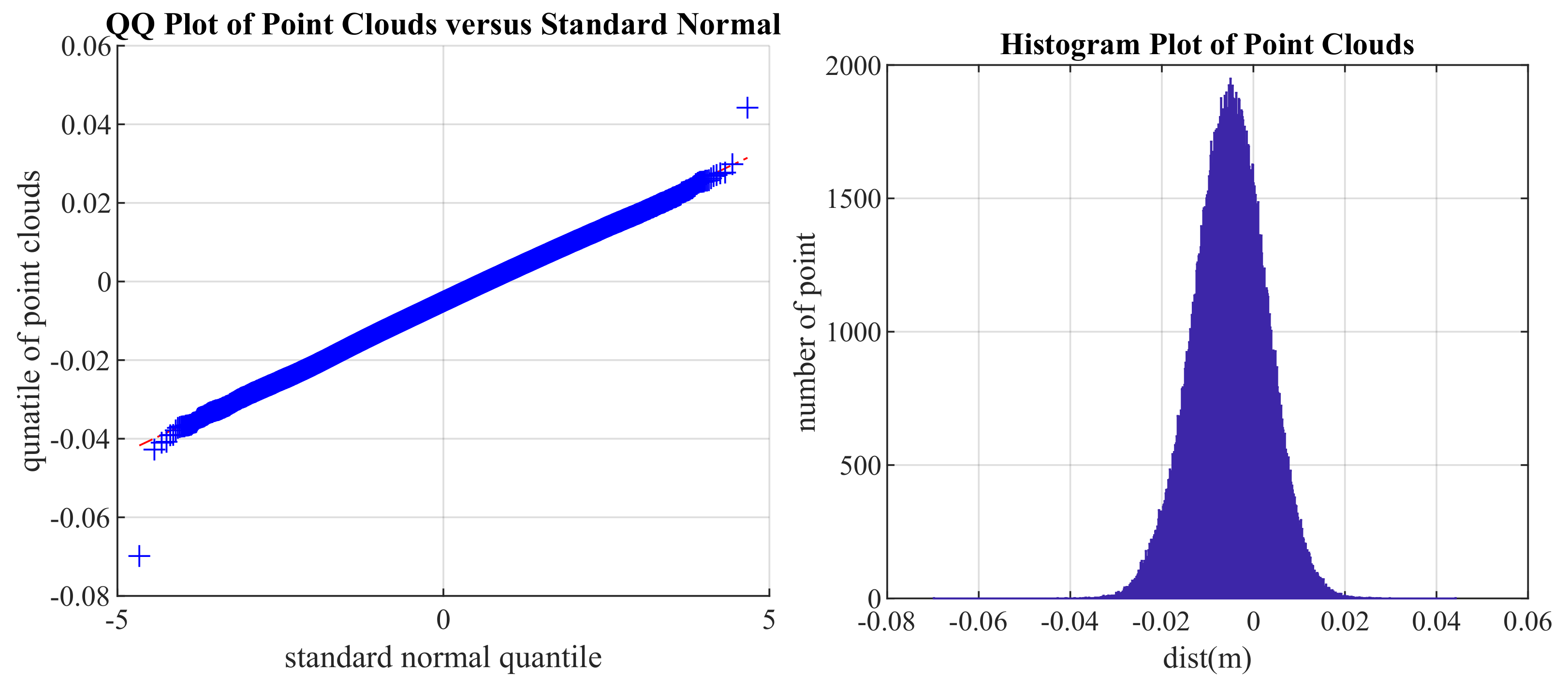
For synthetic data generation, we considered the characteristics of real data such as noise and occlusion. Specifically, we generated all synthetic data to have noise that follows the Gaussian assumption introduced in Section 2.1. In addition, occlusion was introduced by excluding the point clouds of the occluded planes from the point clouds of the cuboid. In addition to noise and occlusion, the density of point clouds was considered because it varies with the SLAM algorithm and the sensor used.
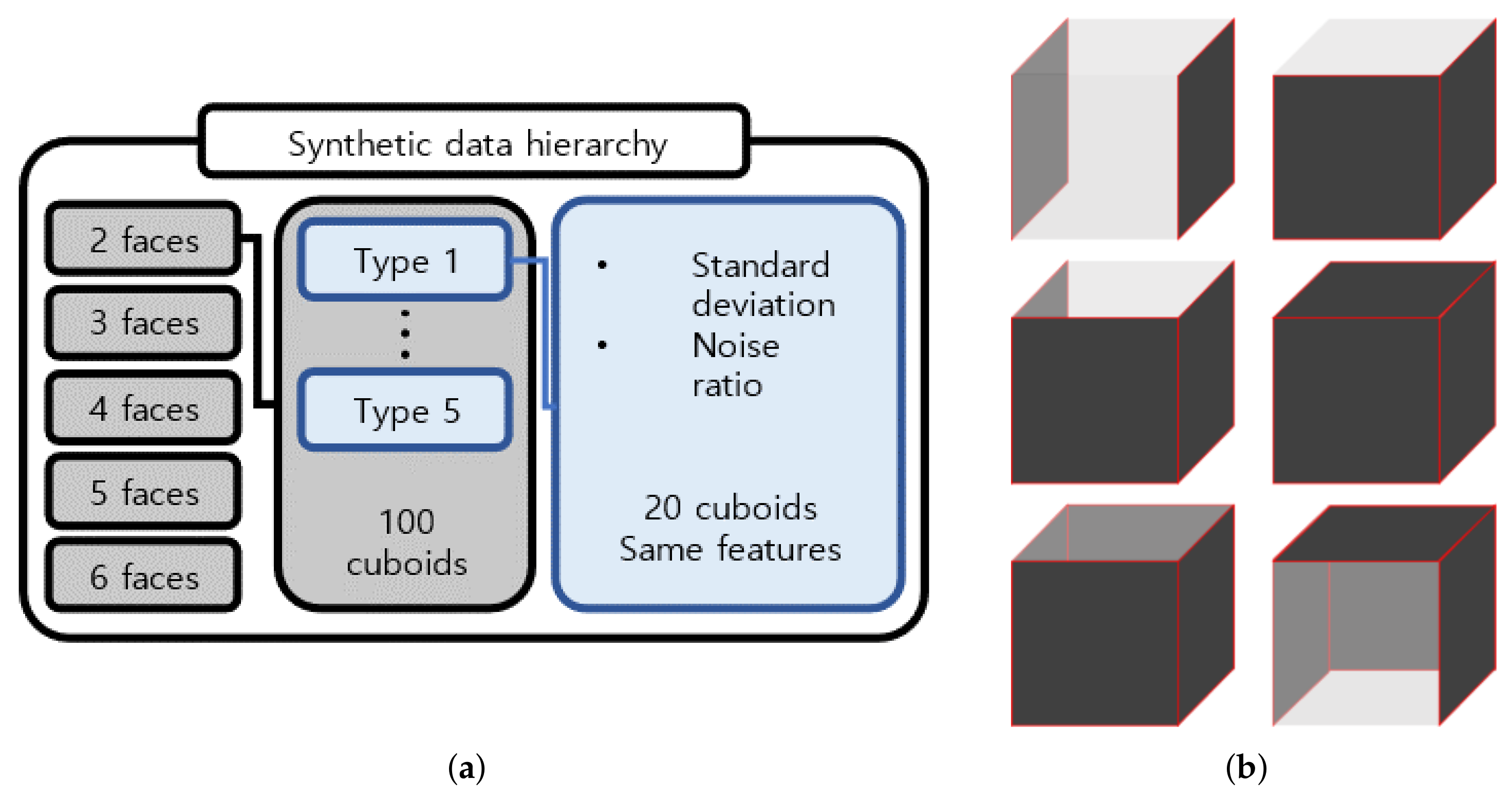
Synthetic data were hierarchically generated, as shown in Figure 6a. First, 500 cuboid data are divided equally into five cases depending on the number of generated faces, because there are no point clouds on the occluded faces. Second, 100 cuboid data of each case are also divided into five types depending on the characteristics related to noise, such as the standard deviation and noise ratio. Here, the standard deviation and noise ratio were arbitrarily taken within ranges of 0.02–0.04 m and 50–100%, respectively. The standard deviation is a parameter of the Gaussian model, and the noise ratio represents the proportion of point clouds following the Gaussian model among all the point clouds of the cuboid. Each cuboid has unique parameters and point density.
To thoroughly evaluate the proposed algorithm, cuboids with 2–6 faces, i.e., the minimum to the maximum number of faces, were created to model a cuboid, even though the measured point clouds generally have a maximum of five faces. Moreover, we included two spatial combinations of reconstructed faces when generating cuboids with 2–4 faces, as shown in Figure 6b.
When Wei et al. [10] generated multiple cuboids, the cost of each cuboid was calculated using the following equation, and the cuboid with the lowest cost was selected.
C o s t = Δ A n g l e × L 2 - norm ( [ Δ S i z e ; Δ C e n t e r ] )
Here, Δ A n g l e ( 1 × 1 ) , Δ S i z e ( 3 × 1 ) , and Δ C e n t e r ( 1 × 1 ) represent the orientation, size, and center error, respectively. Specifically, size error is the absolute difference between the corresponding edges of ground truth. The center error is a two-norm distance between the modeling result and the ground truth. The orientation error is computed as the minimum angle required to transform the obtained orientation to the ground truth orientation.
Robustness is evaluated by the number of correctly modeled cuboids and narrowness of the error range. We counted correctly modeled cuboids by defining an incorrect cuboid model consisting of false and no solutions. The case in which the cuboid parameter estimation fails is determined as no solution, and that in which the estimated parameters have large differences from the ground truth is considered as a false solution. A cuboid model is considered a false solution if any error in the cuboid parameters of size, angle, and center exceeds the threshold. Among the cuboid parameters, we evaluated the size results as the volume, which is the product of each size. This is because it is difficult to achieve consistency in the individual size error results because the error in each size varies depending on the occlusion of the plane of the corresponding axis.
Table 1 reports the cuboid modeling results based on the number of false and no solutions. The threshold was calculated based on the interquartile range of the entire cuboid error generated using the proposed method and that of Wei et al. [10] from the synthetic data. The volume, center, and angle error thresholds were set at 1.5, 1.5, and 5 interquartile ranges, respectively. The units and calculated threshold values are listed in the second row of the table. According to Table 1, in most cases, the proposed method is more robust than the method of Wei et al. [10]. First, there is no case in which the proposed method fails to obtain the cuboid parameters, whereas the method proposed by Wei et al. [10] cannot estimate the cuboid parameters for 50 data in two faces case, which reflects severe occlusion. Second, both the methods accurately estimate the angle of the cuboid; however, the proposed method outperformed the method of Wei et al. [10] in estimating the volume and center for all faces.
The average error between the result parameters and the ground truth, and the number of false and no solutions are listed in Table 2. The average error was calculated using the results of the correctly modeled cuboid. The center and orientation errors were calculated in a manner similar to the selection of the cuboid from multiple results. The volume error was calculated as a percentage, which is the volume of the results divided by the volume of the ground truth. In addition, the units of error are represented in parentheses. The values in bold font indicate better performance, and the hyphen indicates that there is no correctly modeled cuboid.
The proposed method outperformed the method of Wei et al. [10] under most conditions, as shown in Table 2. This suggests that the proposed method can model a cuboid under various noise and occlusion conditions with a lower average error. In some cases, the method of Wei et al. [10] shows better performance than the proposed method, for example, the volume and center error for type 2 in two faces and volume error for type 3 in three faces. However, the proposed method estimates 10 and 5 more cuboids correctly for type 2 in two faces and type 3 in three faces, respectively, compared to the method of Wei et al. [10]. Therefore, it is necessary to match the data used to calculate the average error to accurately compare the error range.
To accurately evaluate the robustness from the perspective of the error range, the average error and standard deviation of the data obtained using both methods are listed in Table 3. In the case of two faces, the data are insufficient to calculate the average and standard deviation because Wei et al. [10] succeeded with only one cuboid. Therefore, the results for the cases of 3–6 faces are provided. The number of cuboids correctly modeled by each method is reported in the used data row.
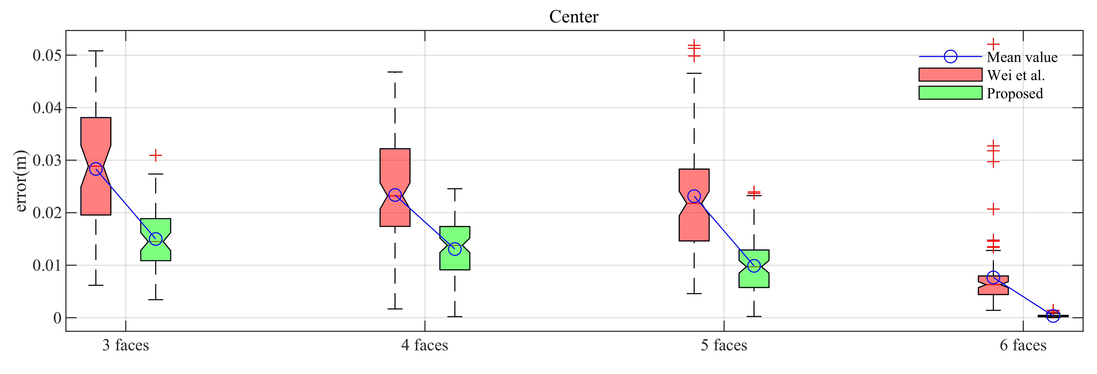
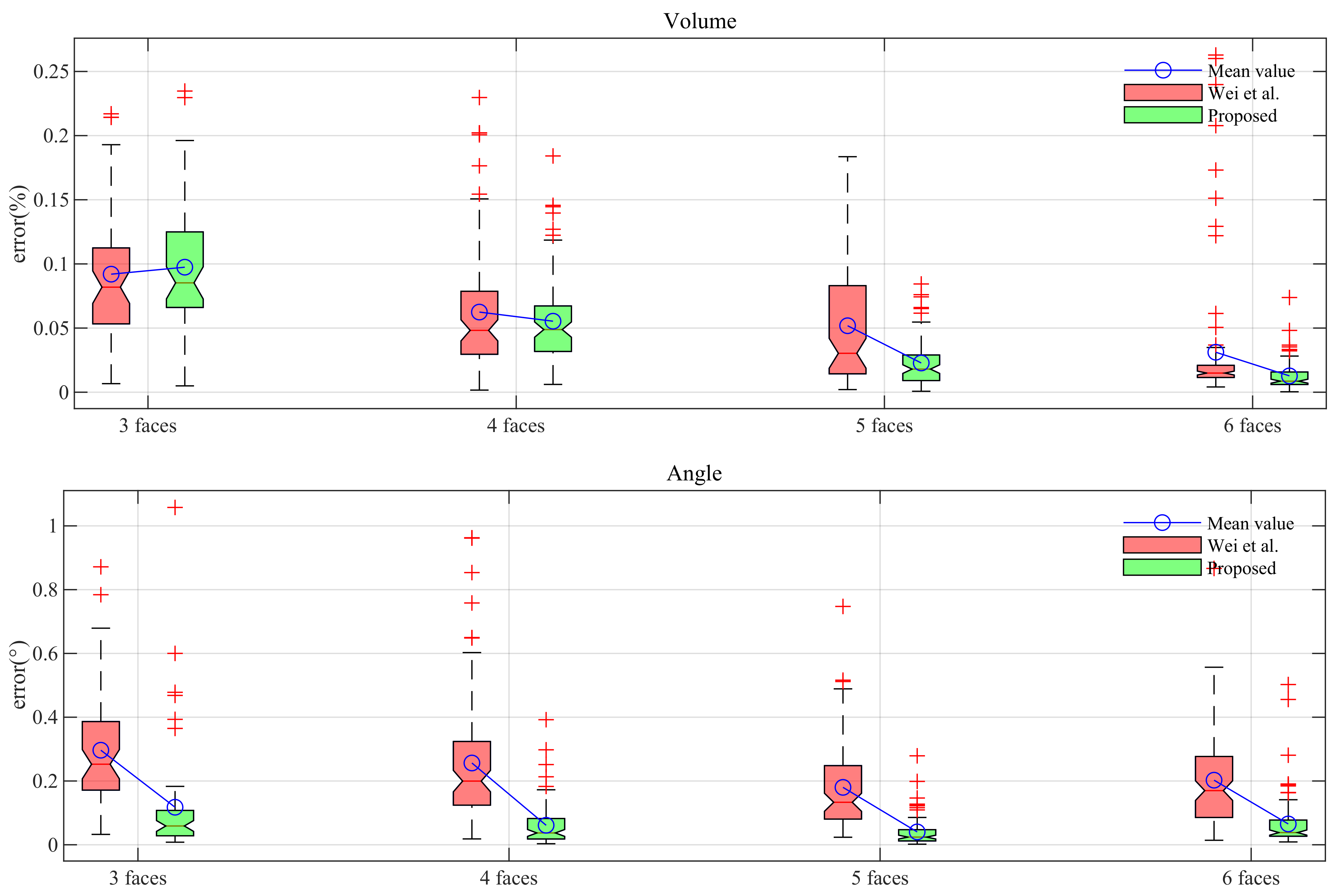
Table 3 lists the mean and standard deviation values of the angle, volume, and center errors for both methods. Based on Table 3, the proposed method achieves smaller mean error and standard deviation for all parameters of the cuboid in most cases. Specifically, the proposed method is more robust than the previously studied method because it achieves a lower and more consistent error for various cases. These results are shown as boxplots in Figure 7 for an easy comparison. Here, the proposed method whose results are colored in green outperforms the previous method whose results are colored in red.

3.3. Real Data

We verified that the proposed method is robust under various noise and occlusion conditions, as discussed in Section 3.2 by comparing its modeling results with the ground truth. Although synthetic data are designed to cover various cases of point clouds, conditions for real data are more difficult. Point clouds measured by the SLAM algorithm are more dynamic than synthetic data. Therefore, real data offers more challenging conditions for the proposed method.
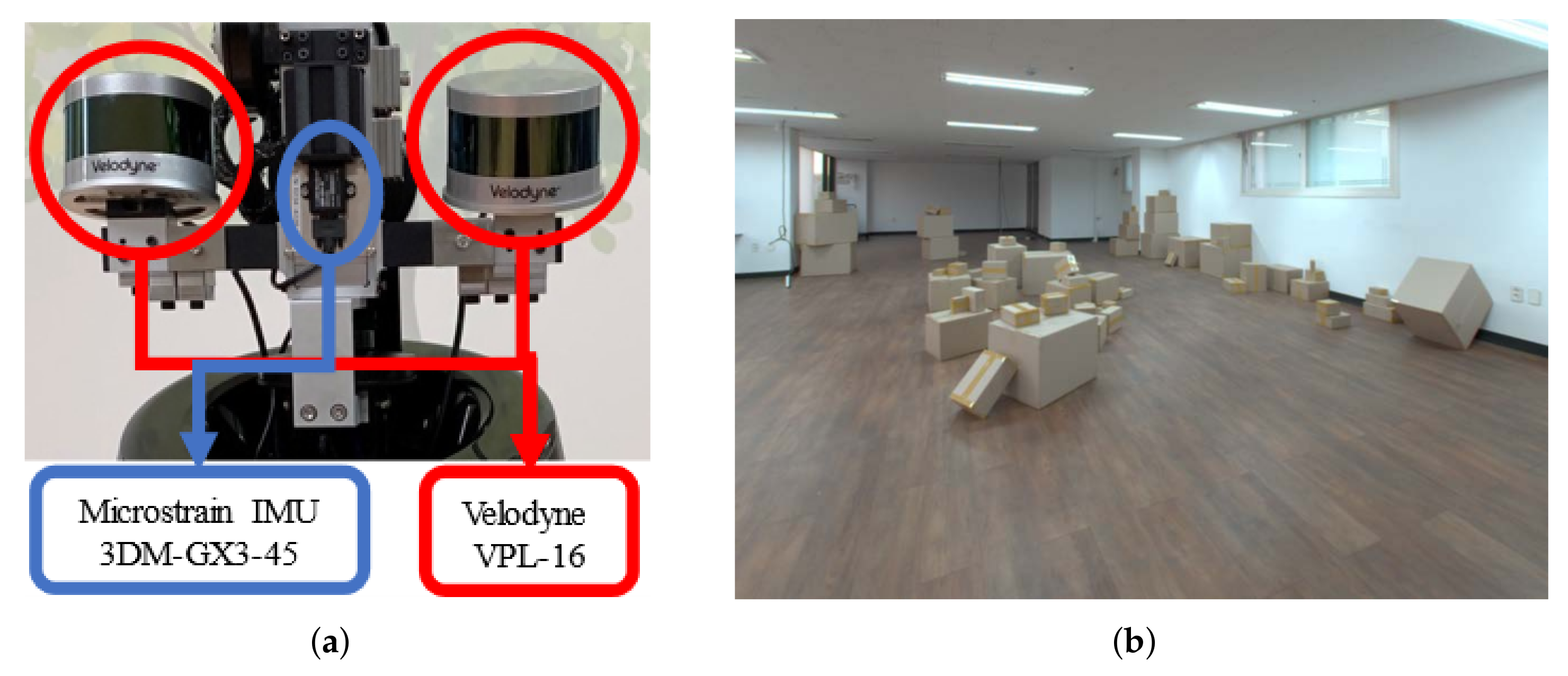
We designed an environment and sensor system for data acquisition. The method of Lee et al. [6] was implemented for the SLAM algorithm to scan the environment, and the sensor system shown in Figure 8a was used to measure the surroundings. We set up a space in which 78 boxes are arbitrarily located, as shown in Figure 8b. The space was scanned five times, and all boxes were randomly rearranged for each scan.
Robustness was evaluated by the number of correctly modeled cuboids and the error range in the synthetic data. However, because there is no ground truth for real data, we used metrics such as P, R, and F, which were used by Wei et al. [10], to evaluate the results instead of the error range. Here, P denotes the number of uniformly sampled point clouds of the cuboid model within a certain distance from the measured point clouds. R represents the number of measured point clouds within a certain distance from the uniformly sampled point clouds of the cuboid model. F represents the harmonic mean of P and R. However, these metrics may be unsuitable for comparing the performance of the cuboid model because the point clouds measured in this study were highly occluded. A practical example of this phenomenon is shown in Figure 9.
Therefore, we developed a metric based on the concept of R score, and the distance between the measured point clouds and uniformly sampled point clouds of the cuboid model. The concept of the R score focuses on the ratio of the number of points located at a certain distance to the total number of points. By contrast, our metric focuses on the distance that makes a certain ratio of points inliers. Specifically, we uniformly sampled points from the cuboid model using an open-source software [28]. Subsequently, we determined the closest distance from the measured point to the sampled point for each measured point. Then, the closest distances were sorted in ascending order. According to this order, k% of points are located near the surface of cuboid modeling results under the k-th percentile distance. Therefore, we obtained the 75th, 80th, and 85th percentile distances to obtain the threshold distances in that 75%, 80%, and 85% of points are located near the surface of the cuboid.
Moreover, we also tested the performance of the proposed method without the Backtracking Line Search on real data to validate the benefits of this step. We noted the performance of the proposed method without the Backtracking Line Search as ‘w/o BTLS’ on Table 4 and Table 5 and Figure 10 to see the enhancement of the robustness.
The robustness was compared based on the number of correctly modeled cuboids and the mean and standard deviation of the results, which were in a manner similar to the synthetic data. The results of the false and no solutions are listed in Table 4. The method of Wei et al. [10] fails to model the correct cuboids for 218 of the total 354 real data, which is approximately 61% of the total cuboid. This percentage is in the middle of the failure rates of the two and three-face cases of the synthetic data, which are 99% and 36%, respectively. Therefore, the condition of real data is difficult. Moreover, this interpretation is supported by the fact that the proposed method yielded two no-solution results for the first time in the experiments. The proposed method without the backtracking line search failed to model the correct cuboids for 47 of the 354 real data. On the other hand, The proposed method with the backtracking line search failed to model the correct cuboids for only 6 of the 354 real data. These real data results show not only a significant improvement over those of the previous method but also the benefit of the backtracking line search. Therefore, it can be concluded that the proposed method is the most robust among other methods under high noise and occlusion conditions.
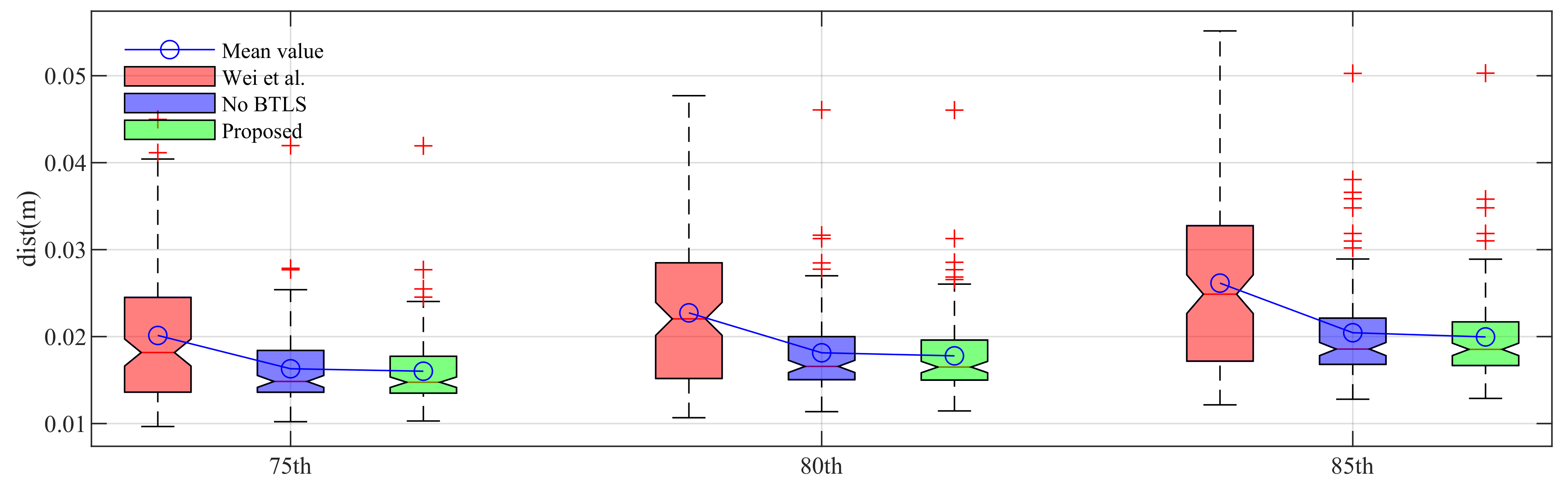
A robustness evaluation based on the distance metric is summarized in Table 5. This table shows that 75, 80, and 85% of the points are distributed at distances within the corresponding values in the table from the surface of the cuboid model. Therefore, we consider that a result with a lower value indicates better performance because the points are located closer to the surface of the cuboid model. Consequently, based on Table 5, the proposed method outperforms other methods in most cases. Specifically, the points are closer to the model surface of the proposed method on average. Moreover, the proposed method achieved consistent results with a lower standard deviation than previous methods. These results are also visualized as boxplots in Figure 10 for easy comparison. Here, the proposed method whose results are colored in green shows an improved performance compared to the previous method whose results are colored in red.

4. Discussion

We verified the robustness of the proposed method through experiments designed to include various tough conditions using synthetic and real data. This was realized from the perspectives of the number of correctly modeled cuboids and the error range. The error range was represented by the mean and standard deviation of the error metric. The difference between the results and the ground truth was used as the error metric for synthetic data, and the distance between the surface of the cuboid model and the point clouds was used as the error metric for real data. The experimental results validated that the proposed method is more robust than a previous method from both perspectives.
In spite of improving the robustness of the proposed method, the limitations of the proposed method are also clear due to the design of the proposed method. Specifically, the proposed method is designed to model a cuboid one by one. Therefore, an appropriate point cloud segment process might be needed to utilize the proposed method as a module of another framework.

5. Conclusions

In this study, we established a robust cuboid modeling method for 3D point clouds with high noise and occlusion. We introduced the GMM concept to directly formulate soft constraints from the point clouds. Specifically, a soft constraint was formulated as an expectation of the GMM. Subsequently, we estimated cuboid parameters using the expectation-maximization scheme, which maximizes the soft constraints. In addition, for accuracy and efficiency, we derived analytic partial derivatives of the soft constraints to calculate the step size during optimization. Thereafter, the parameters of the cuboid model were updated using the backtracking line search method. Lastly, we verified the robustness of the proposed method through experiments designed to include various tough conditions using synthetic and real data.
On the other hand, the limitations of the proposed method still exist as discussed in Section 4. Therefore, to overcome the limitations, there are two future works to consider to enhance the applicability of the proposed method. The first future work is extending the single cuboid modeling to multiple cuboid modeling. If the extension of the proposed method to multiple cuboids is possible, then the proposed method will be more useful in the field of Geometric primitive-based modeling.
The second future work is finding alternative noise model, such as symmetric alpha stable distribution that is the extension of GMM. If another noise model is validated to be suitable for the proposed model, then the proposed method will be utilized with the appropriate model depending on the SLAM algorithm or the sensor system.

Author Contributions

Conceptualization, W.J. and N.D.; methodology, experiments, and analyses, W.J.; writing—original draft preparation, W.J. and J.H.; funding acquisition and writing—review and editing, N.D. All authors have read and agreed to the published version of the manuscript.

Funding

This research was supported by multiple research funds from the Korea Creative Content Agency grant funded by the Ministry of Culture, Sports and Tourism (Project Number: R2022010058) and TeeLabs.

Data Availability Statement

Not applicable.

Conflicts of Interest

The authors declare no conflict of interest.

Appendix A. Linearized Rotation Matrix

In this Appendix, we derive the linearized rotation matrix introduced by Barfoot et al. [29] according to robotics field expressions. This is because the quaternion operations (left-hand and right-hand compounds) used by Barfoot et al. [29] are dissimilar to those in the robotics field, which this study follows. The linearized rotation matrix substitutes the rotation matrix in Equation (13) to update the orientation parameters of the cuboid, as discussed in Section 2.4.1.
The notation and operations of the quaternion are rewritten as follows.
  • Quaternion: q = ϵ η = sin φ 2 × a cos φ 2
  • Inverse of q: q 1 = ϵ η
  • LH Compound: q + = η 1 + ϵ × ϵ ϵ η
  • RH Compound: q = η 1 ϵ × ϵ ϵ η
  • To rotate v: q + v + q 1 = q + q 1 v = C 0 0 1 v
The rotation matrix, C, and its derivative are restated as follows by replacing the corresponding notation and operations of Barfoot et al. [29].
The rotation matrix that rotates φ about the reference axis, a , is as follows.
C ( a , φ ) = ( η 1 + ϵ × ) × ( η 1 ( ϵ ) × ) + ϵ ( ( ϵ ) T ) = cos φ 2 2 1 + 2 cos φ 2 sin φ 2 a × + sin φ 2 2 ( a × a × ( 1 + a a T ) + a a T ) = cos φ 1 + ( 1 cos φ ) a a + sin φ a ×
Differentiating Equation (A1) with respect to φ yields the following equation.
C ( a , φ ) φ = sin φ + sin φ a a T + cos φ a × = sin φ ( 1 + a a T a × a × ) + cos φ a × = sin φ a × a × + ( 1 cos φ ) a × a 0 a T + cos φ a × = a × ( cos φ 1 + ( 1 cos φ ) a a + sin φ a × ) C ( a , φ )
Therefore, the derivatives of the rotation matrix with respect to the Euler angle of the ZYX sequence according to Equation (A2) become
C ( θ ) v θ Z = 1 Z × C ( θ Z ) C ( θ Y ) C ( θ X ) v = ( C ( θ ) v ) × 1 Z C ( θ ) v θ Y = C ( θ Z ) 1 Y × C ( θ Y ) C ( θ X ) v = ( C ( θ ) v ) × C ( θ Z ) 1 Y C ( θ ) v θ X = C ( θ Z ) C ( θ Y ) 1 X × C ( θ X ) v = ( C ( θ ) v ) × C ( θ Z ) C ( θ Y ) 1 X C ( θ ) v θ = C ( θ ) v θ Z C ( θ ) v θ Y C ( θ ) v θ X = ( C ( θ ) v ) × C ( θ Z ) C ( θ Y ) 1 X C ( θ Z ) 1 Y 1 Z S ( θ )
Therefore, the first-order Tayler-series expansion of the rotation matrix is as follows:
C ( θ ¯ + δ θ ) v C ( θ ¯ ) v + C ( θ ) v θ | θ ¯ δ θ = ( 1 + ( S ( θ ) ¯ δ θ ) × ) δ ϕ ( C ( θ ¯ ) v ) = ( 1 + δ ϕ × ) C ( θ ¯ )
Before applying the derived results, we verify Equation (A4), similar to the method proposed by Barfoot et al. [29].
C ( θ ¯ + δ θ ) C ( θ ¯ + δ θ ) ( 1 + δ ϕ × ) C ( θ ¯ ) ( ( 1 + δ ϕ × ) C ( θ ¯ ) ) = 1 δ ϕ × δ ϕ ×
A rotation matrix multiplied by its own transpose produces a 3 × 3 identity matrix and second-order term, which is negated by linearization. This proves that the rotation matrix derived in the robot coordinate system is reasonably linearized. Consequently, we substitute Equation (A4) into Equation (13) to optimize the orientation parameters of a cuboid.

References

  1. Zhang, Y.; Xu, W.; Tong, Y.; Zhou, K. Online Structure Analysis for Real-Time Indoor Scene Reconstruction. ACM Trans. Graph. 2015, 34, 159:1–159:13. [Google Scholar] [CrossRef] [Green Version]
  2. Wang, J.; Oliveira, M.M. Improved Scene Reconstruction from Range Images. Comput. Graph. Forum 2002, 21, 521–530. [Google Scholar] [CrossRef]
  3. Rabbani, T.; Dijkman, S.; van den Heuvel, F.; Vosselman, G. An integrated approach for modelling and global registration of point clouds. ISPRS J. Photogramm. Remote Sens. 2007, 61, 355–370. [Google Scholar] [CrossRef]
  4. Jiang, H.; Xiao, J. A Linear Approach to Matching Cuboids in RGBD Images. In Proceedings of the 2013 IEEE Conference on Computer Vision and Pattern Recognition, Portland, OR, USA, 23–28 June 2013; pp. 2171–2178. [Google Scholar]
  5. Trevor, A.J.B.; Rogers, J.G.; Christensen, H.I. Planar surface SLAM with 3D and 2D sensors. In Proceedings of the 2012 IEEE International Conference on Robotics and Automation, St Paul, MN, USA, 14–18 May 2012; pp. 3041–3048. [Google Scholar]
  6. Lee, K.; Ryu, S.H.; Yeon, S.; Cho, H.; Jun, C.; Kang, J.; Choi, H.; Hyeon, J.; Baek, I.; Jung, W.; et al. Accurate Continuous Sweeping Framework in Indoor Spaces With Backpack Sensor System for Applications to 3-D Mapping. IEEE Robot. Autom. Lett. 2016, 1, 316–323. [Google Scholar] [CrossRef]
  7. Décoret, X.; Durand, F.; Sillion, F.X.; Dorsey, J. Billboard Clouds for Extreme Model Simplification. In Proceedings of the ACM SIGGRAPH 2003 Papers, San Diego, CA, USA, 27–31 July 2003; pp. 689–696. [Google Scholar]
  8. Ren, Z.; Wang, R.; Snyder, J.; Zhou, K.; Liu, X.; Sun, B.; Sloan, P.P.; Bao, H.; Peng, Q.; Guo, B. Real-Time Soft Shadows in Dynamic Scenes Using Spherical Harmonic Exponentiation. In Proceedings of the ACM SIGGRAPH 2006 Papers, Boston, MA, USA, 30 July–3 August 2006; pp. 977–986. [Google Scholar]
  9. Li, Y.; Wu, X.; Chrysathou, Y.; Sharf, A.; Cohen-Or, D.; Mitra, N.J. GlobFit: Consistently Fitting Primitives by Discovering Global Relations. ACM Trans. Graph. 2011, 30, 52:1–52:12. [Google Scholar] [CrossRef]
  10. Wei, Q.; Jiang, Z.; Zhang, H. Robust Spacecraft Component Detection in Point Clouds. Sensors 2018, 18, 933. [Google Scholar] [CrossRef] [PubMed] [Green Version]
  11. Zhou, Y.; Yin, K.; Huang, H.; Zhang, H.; Gong, M.; Cohen-Or, D. Generalized Cylinder Decomposition. ACM Trans. Graph. 2015, 34, 171:1–171:14. [Google Scholar] [CrossRef] [Green Version]
  12. Thiery, J.M.; Guy, E.; Boubekeur, T. Sphere-Meshes: Shape Approximation Using Spherical Quadric Error Metrics. ACM Trans. Graph. 2013, 32, 178:1–178:12. [Google Scholar] [CrossRef]
  13. Shtof, A.; Agathos, A.; Gingold, Y.; Shamir, A.; Cohen-Or, D. Geosemantic Snapping for Sketch-Based Modeling. Comput. Graph. Forum 2013, 32, 245–253. [Google Scholar] [CrossRef]
  14. Mohammadi, M.; Rashidi, M.; Mousavi, V.; Karami, A.; Yu, Y.; Samali, B. Case study on accuracy comparison of digital twins developed for a heritage bridge via UAV photogrammetry and terrestrial laser scanning. In Proceedings of the 10th International Conference on Structural Health Monitoring of Intelligent Infrastructure, Porto, Portugal, 30 June–2 July 2021. [Google Scholar]
  15. Mohammadi, M.; Rashidi, M.; Mousavi, V.; Karami, A.; Yu, Y.; Samali, B. Quality Evaluation of Digital Twins Generated Based on UAV Photogrammetry and TLS: Bridge Case Study. Remote Sens. 2021, 13, 3499. [Google Scholar] [CrossRef]
  16. Mohammadi, M.; Rashidi, M.; Mousavi, V.; Yu, Y.; Samali, B. Application of TLS Method in Digitization of Bridge Infrastructures: A Path to BrIM Development. Remote Sens. 2022, 14, 1148. [Google Scholar] [CrossRef]
  17. Rashidi, M.; Mohammadi, M.; Sadeghlou Kivi, S.; Abdolvand, M.M.; Truong-Hong, L.; Samali, B. A Decade of Modern Bridge Monitoring Using Terrestrial Laser Scanning: Review and Future Directions. Remote Sens. 2020, 12, 3796. [Google Scholar] [CrossRef]
  18. Mishima, M.; Uchiyama, H.; Thomas, D.; Taniguchi, R.i.; Roberto, R.; Lima, J.a.P.; Teichrieb, V. RGB-D SLAM based incremental cuboid modeling. In Proceedings of the European Conference on Computer Vision Workshops, Munich, Germany, 8–14 September 2018; pp. 414–429. [Google Scholar]
  19. Wu, Q.; Xu, K.; Wang, J. Constructing 3D CSG Models from 3D Raw Point Clouds. Comput. Graph. Forum 2018, 37, 221–232. [Google Scholar] [CrossRef]
  20. Hu, H.; Immel, F.; Janosovits, J.; Lauer, M.; Stiller, C. A Cuboid Detection and Tracking System using A Multi RGBD Camera Setup for Intelligent Manipulation and Logistics. In Proceedings of the 2021 IEEE 17th International Conference on Automation Science and Engineering, Lyon, France, 23–27 August 2021; pp. 1097–1103. [Google Scholar]
  21. Fischler, M.A.; Bolles, R.C. Random Sample Consensus: A Paradigm for Model Fitting with Applications to Image Analysis and Automated Cartography. Commun. ACM 1981, 24, 381–395. [Google Scholar] [CrossRef]
  22. Borrmann, D.; Elseberg, J.; Lingemann, K.; Nüchter, A. The 3D Hough Transform for plane detection in point clouds: A review and a new accumulator design. 3D Res. 2011, 2, 1–3. [Google Scholar] [CrossRef]
  23. Reynolds, D. Gaussian Mixture Models. In Encyclopedia of Biometrics; Li, S.Z., Jain, A., Eds.; Springer: Boston, MA, USA, 2009; pp. 659–663. ISBN 978-0-387-73003-5. [Google Scholar]
  24. Öner, M.; Deveci Kocakoç, I. JMASM 49: A compilation of some popular goodness of fit tests for normal distribution: Their algorithms and MATLAB codes (MATLAB). J. Mod. Appl. Stat. Methods 2017, 16, 547–575. [Google Scholar] [CrossRef]
  25. Moon, T. The expectation-maximization algorithm. IEEE Signal Process. Mag. 1996, 13, 47–60. [Google Scholar] [CrossRef]
  26. Van den Bos, A. Appendix C: Positive Semidefinite and Positive Definite Matrices. In Parameter Estimation for Scientists and Engineers; John Wiley & Sons, Ltd.: West Sussex, UK, 2007; pp. 259–263. ISBN 978-0-470-17386-2. [Google Scholar]
  27. Korsawe, J. MATLAB Central File Exchange. Available online: https://www.mathworks.com/matlabcentral/fileexchange/18264-minimal-bounding-box (accessed on 24 February 2022).
  28. Prakhar. MATLAB Central File Exchange. Available online: https://www.mathworks.com/matlabcentral/fileexchange/54778-sample3d-vertices-faces-n (accessed on 24 February 2022).
  29. Barfoot, T.; Forbes, J.R.; Furgale, P.T. Pose estimation using linearized rotations and quaternion algebra. Acta Astronaut. 2011, 68, 101–112. [Google Scholar] [CrossRef]
Figure 1. Comparison of cuboid modeling procedures. (a) Previous cuboid modeling method. Each hard constraint imposing process narrows solution space. (b) Proposed cuboid modeling method with GMM. Initial guess is iteratively optimized through the soft constraint that assigns score to solution space.
Remotesensing 14 05035 g001
Figure 2. Point clouds noise models and point clouds distribution assumption. Green-filled dots are reconstructed point clouds. Black-empty dots represent ideal measurements. (a) Two types of noise models. The upper example shows the noise model with sensor error. Point clouds acquired by LiDAR sensor are not aligned owing to sensor error. The lower example shows the noise model with motion error. Point clouds acquired from true position of LiDAR sensor (gray) are shifted owing to the position of LiDAR sensor with motion error (thick circle). (b) Gaussian assumption of point clouds distribution generated by noise model shown in (a).
Remotesensing 14 05035 g002
Figure 3. Quantile–Quantile Plot (Left) and Histogram (Right) of distances between points and measured plane.
Remotesensing 14 05035 g003
Figure 4. Backtracking line search implementation. (a) The first step size of parameter update is colored in red. When the soft constraint values of the updated parameters are smaller than previous ones, (b) step size is reduced by half. Modified step size is colored in blue. When the soft constraint values of the updated parameters are greater than previous ones, (c), parameters are updated.
Remotesensing 14 05035 g004
Figure 5. Types of multiple cuboid modeling from point clouds of a single cuboid by Wei et al. [10]. (ac) Arbitrarily chosen synthetic data with which multiple cuboids are generated and (df) corresponding modeling results. (a,d) Case in which multiple cuboids of slightly different sizes are overlapped. (b,e) Case in which one plane is modeled as a cuboid and the remainder point clouds are modeled as another cuboid. (c,f) Case in which each plane is modeled as a cuboid.
Remotesensing 14 05035 g005
Figure 6. Synthetic data generation (a) Hierarchy of synthetic data. Total 500 synthetic cuboid point clouds are hierarchically generated as above. This figure illustrates the configuration of synthetic cuboid data containing two faces. Synthetic cuboid data with the same number of faces are composed of five types of cuboids. Each type of cuboid consists of 20 cuboids with same point deviations and point noise ratio that is randomly selected. Cuboids with different number of faces have same configurations. (b) Two types of cuboid models with same number of occluded faces. There are two combinations of cuboids with (top row) two faces, (middle row) three faces, and (bottom row) four faces, depending on their spatial relations. The dark face represents the surface where point clouds are reconstructed.
Remotesensing 14 05035 g006
Figure 7. Boxplot of results reported in Table 3. Symbols representing method of Wei et al. [10] and proposed method are colored in red and green, respectively. Mean errors of two methods are denoted as blue lines with circle markers, respectively, to visualize results reported in Table 3.
Remotesensing 14 05035 g007aRemotesensing 14 05035 g007b
Figure 8. Real data acquisition setting. (a) Sensor system configuration. Sensor system used to acquire point clouds is consisting of two Velodyne VLP-16 channels and Microstrain 3DX-GX3-45 model. (b) Environment in which SLAM is executed to obtain real point cloud data of cuboid.
Remotesensing 14 05035 g008
Figure 9. P, R, and F scores of the cuboid model obtained by Wei et al. [10] and proposed method. Although the results of Wei et al. [10], colored in red cuboid, do not cover most point clouds, higher scores are obtained in P and F metrics, and the proposed method yields higher score only in the R metric.
Remotesensing 14 05035 g009
Figure 10. Boxplots of results with succeeded data using triple methods summarized in Table 5. The method of Wei et al. [10], the proposed method without Backtracking Line Search step, and the proposed method are colored in red, blue, and green, respectively. Mean distances of triple methods are denoted as blue lines and circle markers, respectively, to visualize the results of Table 5.
Remotesensing 14 05035 g010
Table 1. Number of false and no solutions for synthetic data.
No Solution (#)False Solution (#)Total (#)
Threshold--Angle ( )1.6959Volume (%)0.2707Center (m)0.0545--
MethodWei et al.ProposedWei et al.ProposedWei et al.ProposedWei et al.ProposedWei et al.Proposed
2 faces5001149264979926
3 faces101026143003614
4 faces00004180121
5 faces10105090140
6 faces0000404050
Table 2. Performance comparison depending on noise and occlusion condition.
2 facesType 1Type 2Type 3Type 4Type 5
Noise ratio (%)57.768269.123552.004795.221177.8355
Standard deviation (m)0.03450.03000.02540.02340.0226
MethodsWei et al.ProposedWei et al.ProposedWei et al.ProposedWei et al.ProposedWei et al.Proposed
Angle ( )-0.15100.31170.1800-0.1207-0.1083-0.2585
Volume (%)-12.31068.191611.3878-10.3600-8.0948-7.0110
Center (m)-0.02390.01590.0177-0.0133-0.0160-0.0121
No solution (#)8010011090120
False solution (#)126999311484
3 facesType 1Type 2Type 3Type 4Type 5
Noise ratio (%)74.452778.289068.100275.966452.8059
Standard deviation (m)0.02700.03950.03010.02960.0258
MethodsWei et al.ProposedWei et al.ProposedWei et al.ProposedWei et al.ProposedWei et al.Proposed
Angle ( )0.42370.16580.43160.15870.32970.18560.27140.06750.28420.1065
Volume (%)12.316812.101114.892010.90646.98758.92267.97838.647310.28188.5232
Center (m)0.02150.01400.03180.02480.03630.01650.03330.01910.01890.0111
No solution (#)1000000000
False solution (#)26161728322
4 facesType 1Type 2Type 3Type 4Type 5
Noise ratio (%)86.699679.097288.498557.373268.4000
Standard deviation (m)0.02120.02470.02330.02230.0390
MethodsWei et al.ProposedWei et al.ProposedWei et al.ProposedWei et al.ProposedWei et al.Proposed
Angle ( )0.25140.06910.29420.07540.27340.04350.13770.04790.40770.1068
Volume (%)5.36745.08266.98586.19366.17565.25805.53004.91709.46586.3098
Center (m)0.02210.01220.02740.01150.02230.01490.01840.01200.03220.0169
No solution (#)0000000000
False solution (#)00110000110
5 facesType 1Type 2Type 3Type 4Type 5
Noise ratio (%)71.965854.103688.260490.629450.4478
Standard deviation (m)0.02820.02600.03290.02070.0394
MethodsWei et al.ProposedWei et al.ProposedWei et al.ProposedWei et al.ProposedWei et al.Proposed
Angle ( )0.16090.11240.12910.04650.16870.04530.20140.04580.24240.0393
Volume (%)5.97363.44934.19282.68336.83931.85854.30381.76825.46782.5914
Center (m)0.01980.00850.01990.00680.02860.01300.01730.00860.03390.0123
No solution (#)1000000000
False solution (#)1000900030
6 facesType 1Type 2Type 3Type 4Type 5
Noise ratio (%)95.205690.659357.537297.851180.7944
Standard deviation (m)0.02070.03830.03900.02160.0316
MethodsWei et al.ProposedWei et al.ProposedWei et al.ProposedWei et al.ProposedWei et al.Proposed
Angle ( )0.18190.05760.27410.10720.15750.08440.22710.05300.17700.0687
Volume (%)2.81481.45833.94451.83642.46201.30332.92981.46583.48361.2712
Center (m)0.00870.00030.00890.00060.00750.00040.00540.00020.00780.0003
No solution (#)0000000000
False solution (#)0020101010
Table 3. Error mean and standard deviation with same data.
3 Faces4 Faces5 Faces6 Faces
MethodsWei et al.ProposedWei et al.ProposedWei et al.ProposedWei et al.Proposed
AngleMean0.29650.11770.25640.06120.18000.04030.20250.0653
( )Standard deviation0.17660.18250.19890.06620.13850.04500.16340.0782
VolumeMean0.09200.09740.06250.05530.05180.02280.03120.0127
(%)Standard deviation0.05650.05040.05020.03480.04990.01830.05260.0111
CenterMean0.02830.01500.02340.01310.02310.00990.00770.0003
(m)Standard deviation0.01200.00610.01120.00570.01090.00560.00710.0002
Used data (#)54878695
Table 4. Number of false and no solutions for real data.
No Solution (#)False Solution (#)Total (#)
Threshold-75th (m)0.045480th (m)0.050985th (m)0.0578-
Wei et al.154465064218
w/o BTLS2918181547
Proposed24426
Table 5. Performance comparison based on distance metric.
Results with Succeeded Data by Each Method
percentiles75th80th85thUsed data
mean (m)std (m)mean (m)std (m)mean (m)std (m)(#)
Wei et al.0.01980.00760.02240.00840.02590.0102136
w/o BTLS0.02110.00730.02310.00790.02560.0085307
Proposed0.02050.00710.02260.00760.02500.0082348
Results with Succeeded Data by Both Methods
percentiles75th80th85thUsed data
mean (m)std (m)mean (m)std (m)mean (m)std (m)(#)
Wei et al.0.02010.00780.02270.00860.02610.0104
w/o BTLS0.01630.00430.01810.00480.02040.0056121
Proposed0.01600.00410.01780.00450.02000.0051
Publisher’s Note: MDPI stays neutral with regard to jurisdictional claims in published maps and institutional affiliations.

