

Investigation of Absorption Bands around 3.3 μm in CRISM Data

Abstract
:
1. Introduction
- (1)
- In June 2019, the CH4 abundance on Mars’s surface was estimated at approximately 20 ppbv by SAM-TLS [17], and the distance of the Curiosity rover from the source of the detected spike was unknown.
- (2)
- (3)
- The time of survival of CH4 in the atmosphere spans from hours to 300 years [26].
- (4)
- Since August 2012, Curiosity has detected only two methane spikes, during 2013 and 2019. Assuming, in our work, that these sudden increases in methane concentration were sporadic, we looked for CH4 absorption that would eventually correspond to spikes in CH4 at the scene; that is, a concentration of methane greater than the values found for the background at tens/hundreds of ppb. Consequently, we expected to eventually observe few featured pixels/no featured pixels in the greater part of the investigated images.
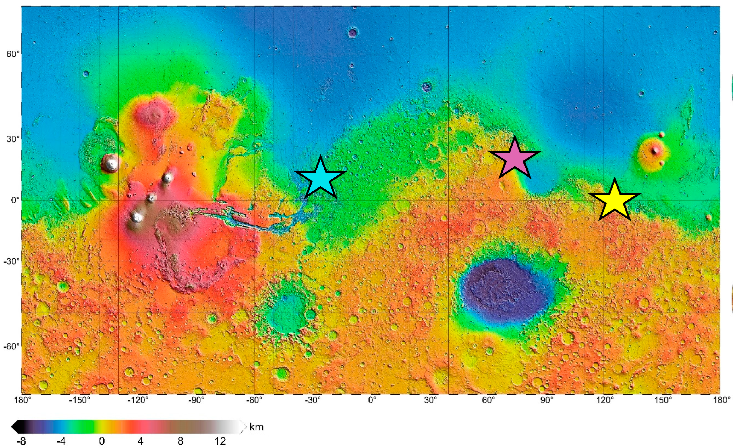
Area Selection
2. Data and Methods
2.1. CRISM Data Processing
2.2. Processing of 3.3 μm Absorption
2.3. Noise Estimation and Choice of the Thresholds
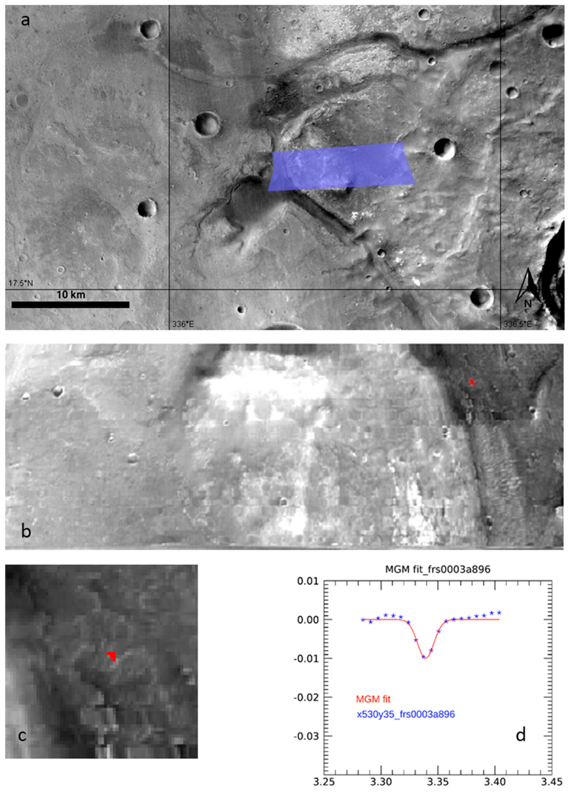
2.4. Mars’s Surface Modeling
3. Results
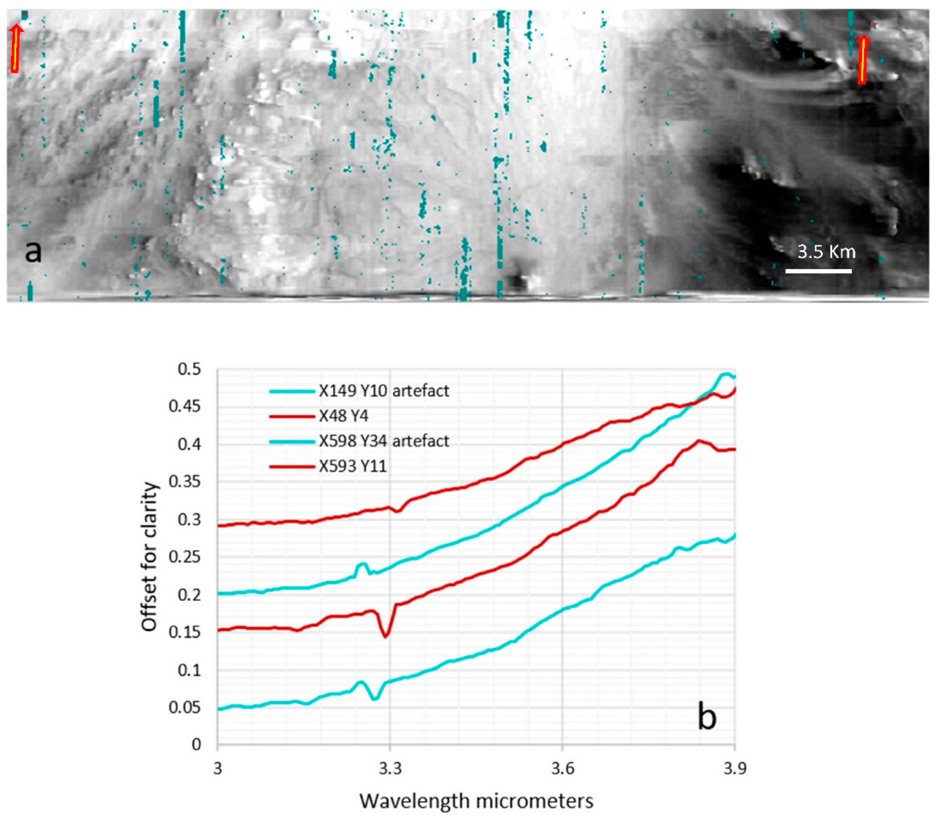
3.1. Spectral Investigation of CRISM I/F Observations
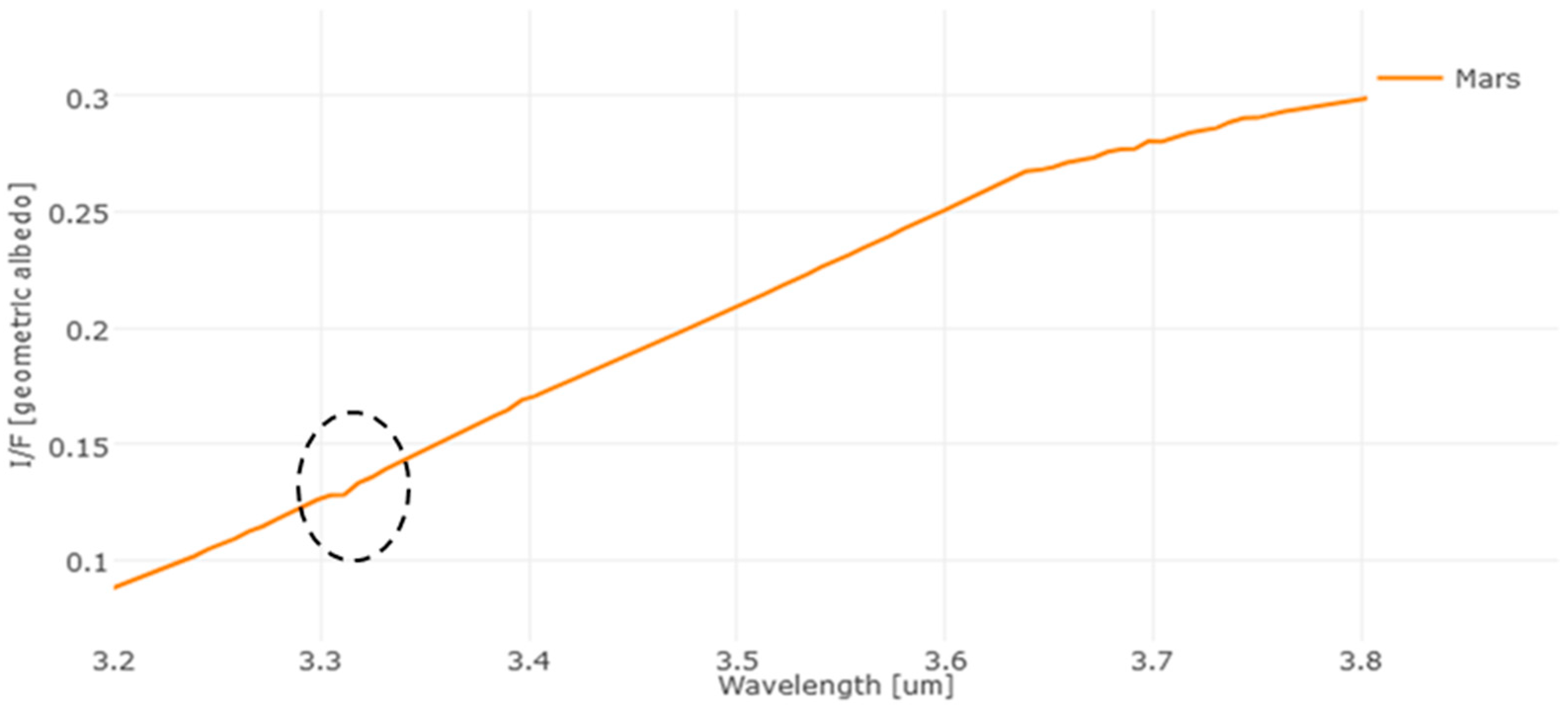
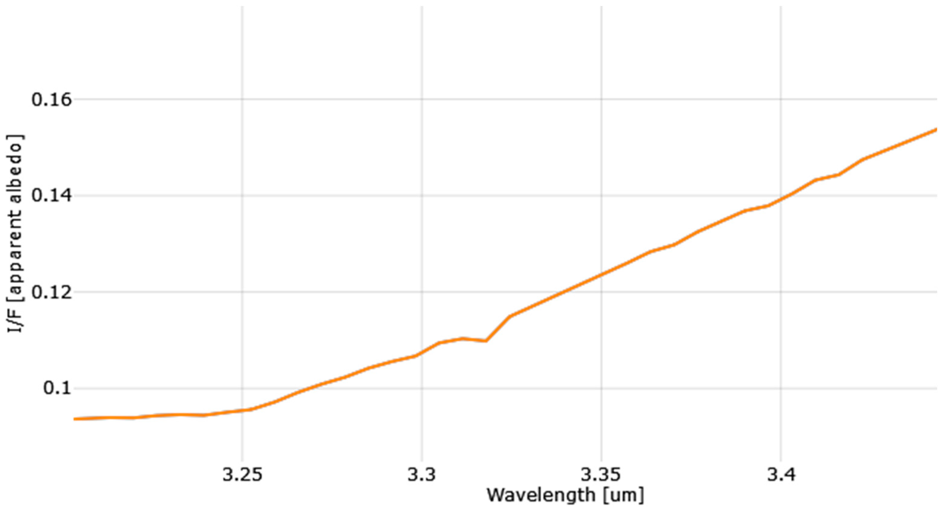
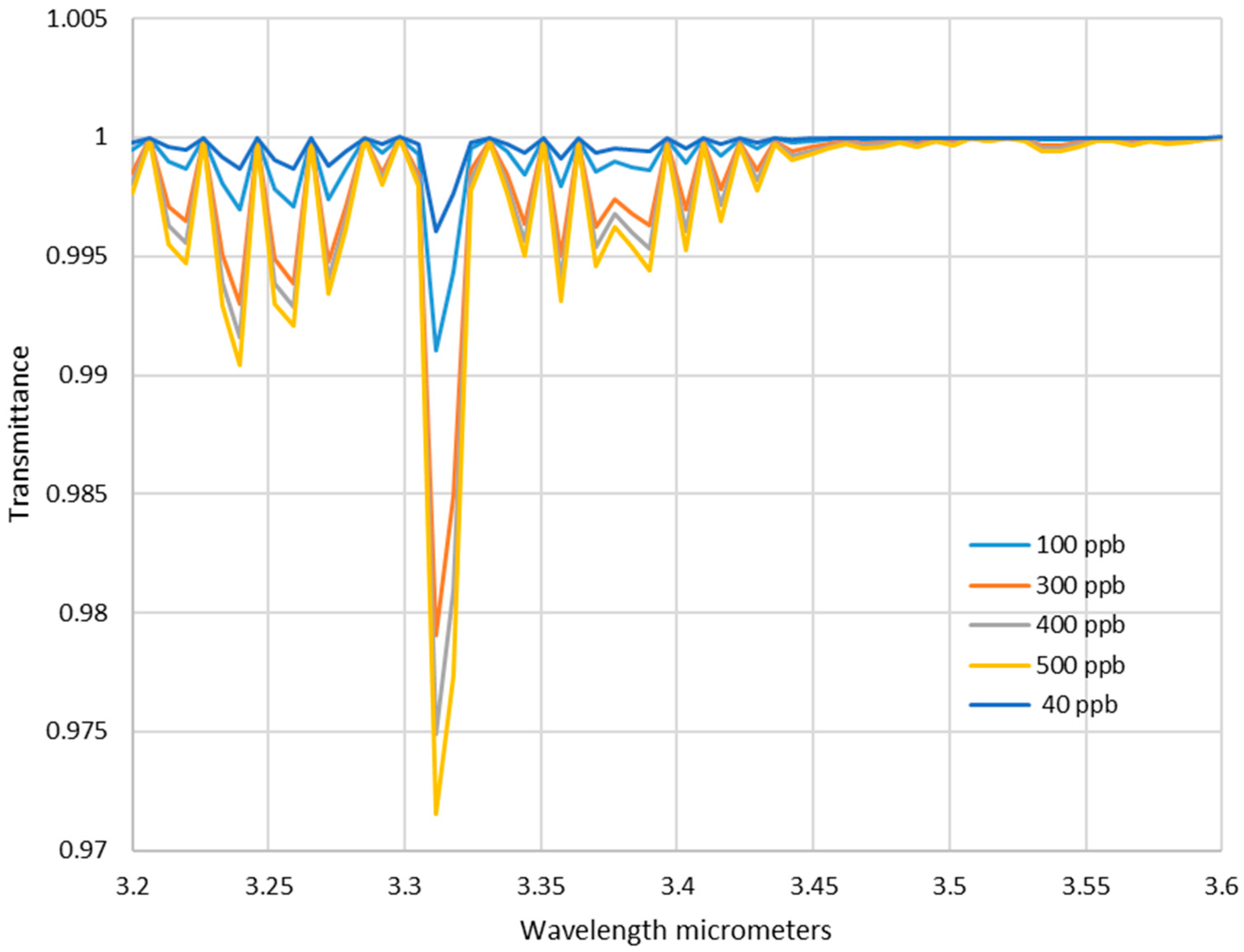
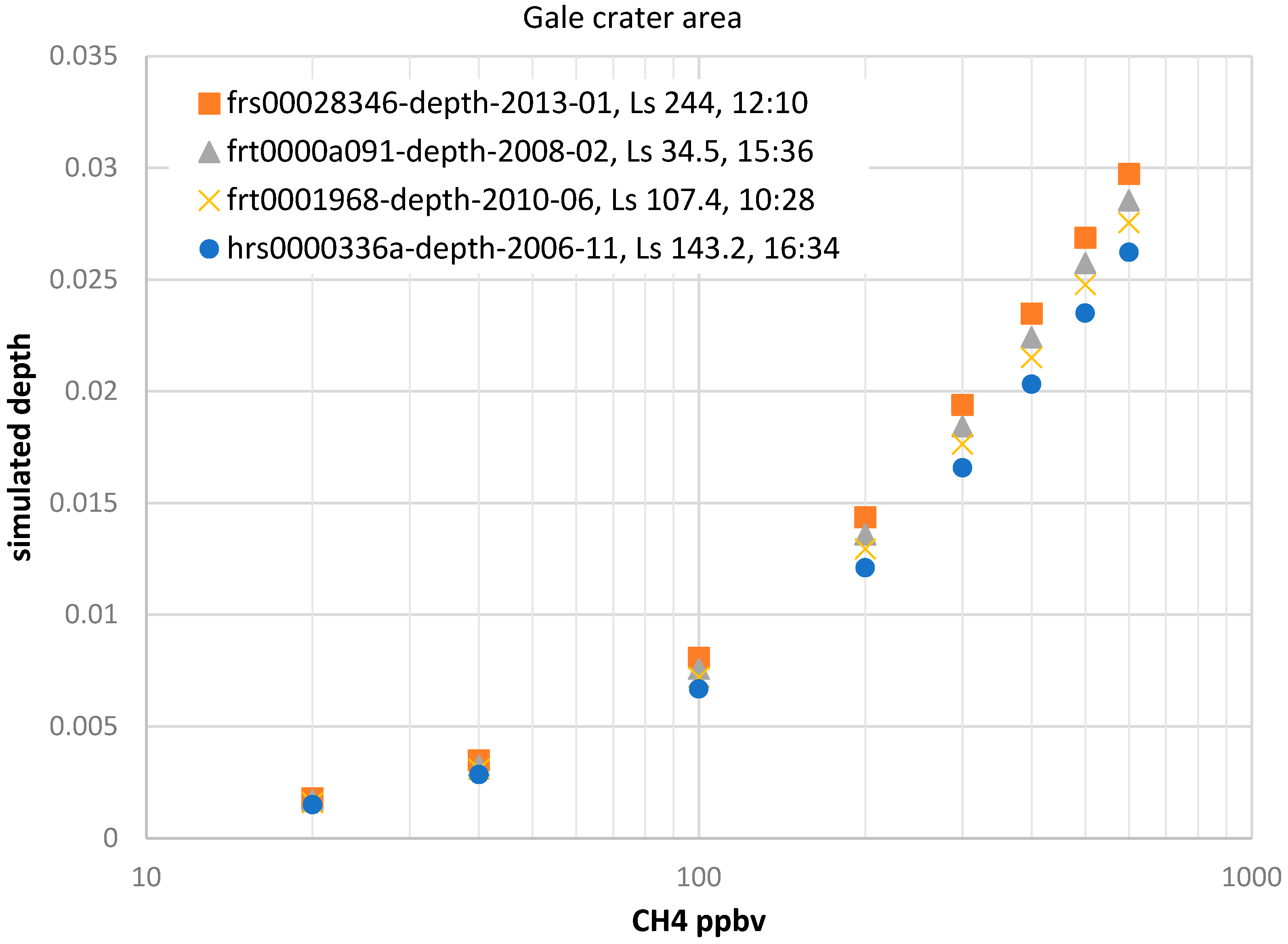
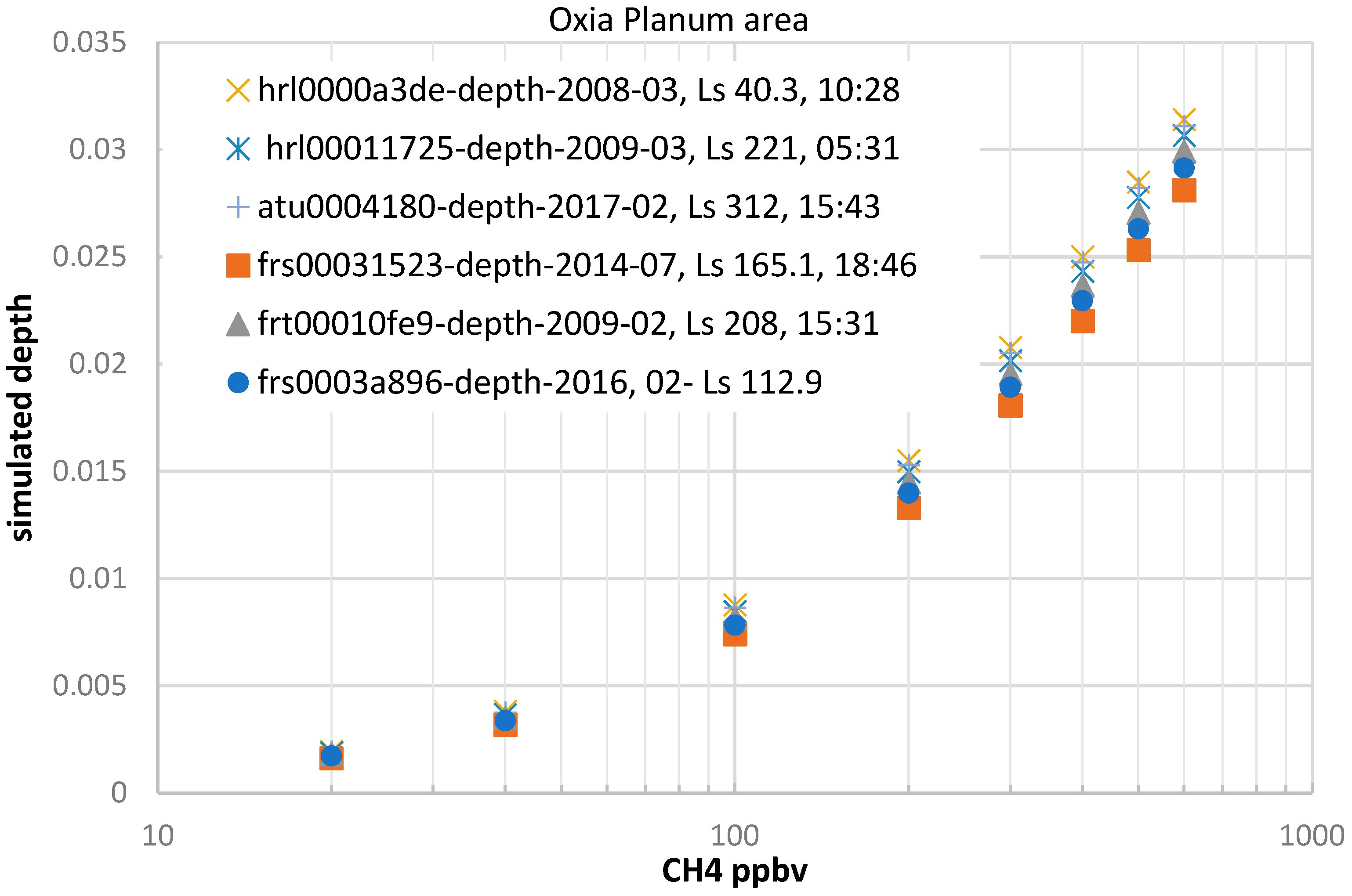
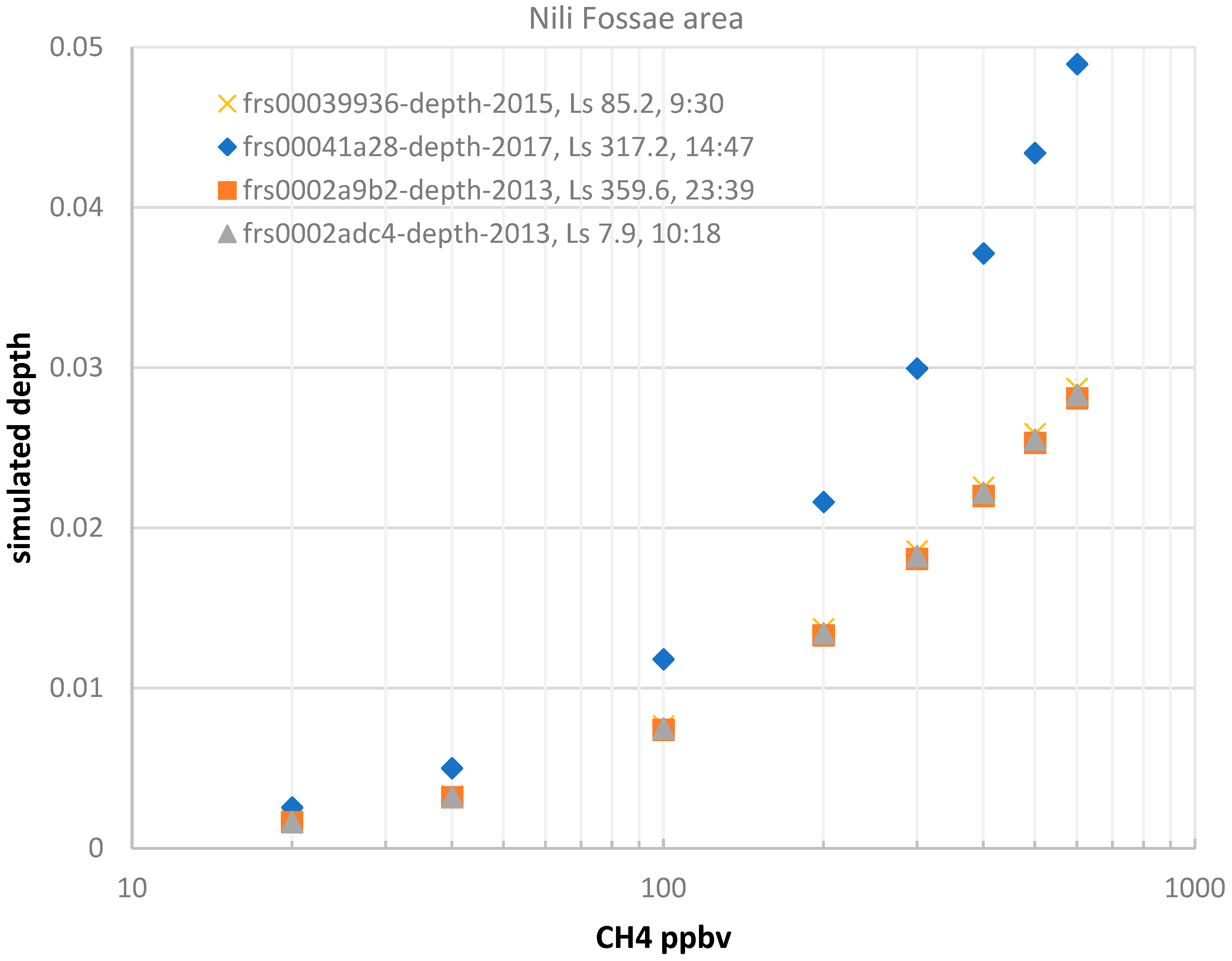
3.2. Simulated Spectrum of Methane Gas on Mars’s Surface
4. Discussion
4.1. Good Candidates but Artifacts
4.2. Good Candidates, Potential Methane Spikes?
4.3. Organic Matter and PAHs
5. Conclusions
Supplementary Materials
Author Contributions
Funding
Data Availability Statement
Conflicts of Interest
References
- Pavlov, A.A.; Hurtgen, M.T.; Kasting, J.F.; Arthur, M.A. Methane-rich Proterozoic atmosphere. Geology 2003, 31, 87–90. [Google Scholar] [CrossRef]
- Etiope, G.; Oehler, D.Z.; Allen, C.C. Methane emissions from Earth’s degassing: Implications for Mars. Planet. Space Sci. 2011, 59, 182–195. [Google Scholar] [CrossRef]
- Etiope, G.; Sherwood Lollar, B. Abiotic Methane on Earth. Rev. Geophys. 2013, 51, 276–299. [Google Scholar] [CrossRef]
- Oze, C.; Sharma, M. Have olivine, will gas: Serpentinization and the abiogenic production of methane on Mars. Geophys. Res. Lett. 2005, 32, L10203. [Google Scholar] [CrossRef] [Green Version]
- Meslin, P.-Y.; Gough, R.; Lefèvre, F.; Forget, F. Little variability of methane on Mars induced by adsorption in the regolith. Planet. Space Sci. 2011, 59, 247–258. [Google Scholar] [CrossRef]
- Gough, R.V.; Tolbert, M.A.; McKay, C.P.; Toon, O.B. Methane adsorption on a martian soil analog: An abiogenic explana-tion for methane variability in the martian atmosphere. Icarus 2010, 207, 165–174. [Google Scholar] [CrossRef]
- Chassefière, E. Metastable methane clathrate particles as a source of methane to the martian atmosphere. Icarus 2009, 204, 137–144. [Google Scholar] [CrossRef]
- Atreya, S.K.; Mahaffy, P.R.; Wong, A.S. Methane and related species on Mars: Origin, loss, implications for life and habitability. Planet. Space Sci. 2007, 55, 358–369. [Google Scholar] [CrossRef]
- Mumma, M.J.; Novak, R.E.; DiSanti, M.A.; Bonev, B.P.; Dello Russo, N. Detection and mapping of methane and water on Mars. Am. Astron. Soc. DPS Meet. 2004, 36, 1127. [Google Scholar]
- Mumma, M.J.; Villanueva, G.L.; Novak, R.E.; Hewagama, T.; Bonev, B.P.; DiSanti, M.A.; Mandell, A.M.; Smith, M.D. “Strong Release of Methane on Mars in Northern Summer 2003”. Science 2009, 323, 1041–1045. [Google Scholar] [CrossRef] [PubMed] [Green Version]
- Krasnopolsky, A.; Maillard, J.P.; Owen, T.C. Detection of methane in the Martian atmosphere: Evidence for life? Icarus 2004, 172, 537–547. [Google Scholar] [CrossRef]
- Formisano, V.; Atreya, S.; Encrenaz, T.; Ignatiev, N.; Giuranna, M. Detection of Methane in the Atmosphere of Mars. Science 2004, 306, 1758–1761. [Google Scholar] [CrossRef] [Green Version]
- Korablev, O.; Vandaele, A.C.; Montmessin, F.; the ACS and NOMAD Science Teams. No detection of methane on mars from early Exomars Trace Gas Orbiter obser-vations. Nature 2019, 568, 517. [Google Scholar] [CrossRef] [PubMed]
- Webster, C.R.; Mahaffy, P.R.; Atreya, S.K.; Flesch, G.J.; Mischna, M.A.; Meslin, P.-Y.; Farley, K.A.; Conrad, P.G.; Christensen, L.E.; Pavlov, A.A.; et al. Mars methane detection and variability at Gale crater. Science 2015, 347, 415–417. [Google Scholar] [CrossRef] [PubMed] [Green Version]
- Webster, C.R.; Mahaffy, P.R.; Atreya, S.K.; Moores, J.E.; Flesch, G.J.; Malespin, C.; Martinez, G.; SmithJavier, C.L.; Martin-Torres, J.; Gomez-Elvira, J.; et al. Background levels of me-thane in Mars’ atmosphere show strong seasonal variations. Science 2018, 360, 1093–1096. [Google Scholar] [CrossRef] [PubMed] [Green Version]
- Webster, C.R.; Mahaffy, P.R.; Pla-Garcia, J.; Rafkin, S.C.R.; Moores, J.E.; Atreya, S.K.; Flesch, G.J.; Malespin, C.A.; Teinturier, S.M.; Kalucha, H.; et al. Day-night differences in Mars methane suggest nighttime containment at Gale crater. Astron. Astrophys. 2021, 650, A166. [Google Scholar] [CrossRef]
- Moores, J.E.; King, P.L.; Smith, C.L.; Martinez, G.M.; Newman, C.E.; Guzewich, S.D.; Meslin, P.; Webster, C.R.; Mahaffy, P.R.; Atreya, S.K.; et al. The methane diurnal variation and microseepage flux at Gale crater, Mars as constrained by the ExoMars Trace Gas Orbiter and Curiosity observations. Geophys. Res. Lett. 2019, 46, 9430–9438. [Google Scholar] [CrossRef]
- Guzewich, S.D.; Newman, C.E.; Smith, M.D.; Moores, J.E.; Smith, C.L.; Moore, C.; Richardson, M.I.; Kass, D.; Kleinböhl, A.; Mischna, M.; et al. The Vertical Dust Profile Over Gale Crater, Mars. J. Geophys. Res. Planets 2017, 122, 2779–2792. [Google Scholar] [CrossRef]
- Giuranna, M.; Viscardy, S.; Daerden, F.; Neary, L.; Etiope, G.; Oehler, D.Z.; Formisano, V.; Aronica, A.; Wolkenberg, P.; Aoki, S.; et al. Independent confirmation of a methane spike on Mars and a source region east of Gale Crater. Nat. Geosci. 2019, 12, 326–332. [Google Scholar] [CrossRef]
- Yung, Y.L.; Chen, P.; Nealson, K.; Atreya, S.; Beckett, P.; Blank, J.G.; Ehlmann, B.; Eiler, J.; Etiope, G.; Ferry, J.G.; et al. Methane on Mars and Habitability: Challenges and Responses. Astrobiology 2018, 18, 1221–1242. [Google Scholar] [CrossRef]
- Etiope, G. Natural Gas Seepage. In The Earth’s Hydrocarbon Degassing; Springer: Berlin/Heidelberg, Germany, 2015; p. 199. [Google Scholar]
- Oehler, D.Z.; Etiope, G. Methane Seepage on Mars: Where to Look and Why. Astrobiology 2017, 17, 1233–1264. [Google Scholar] [CrossRef] [PubMed]
- Etiope, G.; Oehler, D.Z. Methane spikes, background seasonality and non-detections on Mars: A geological perspective. Planet. Space Sci. 2019, 168, 52–61. [Google Scholar] [CrossRef]
- MacKinnon, D.J.; Tanaka, K.L. The impact martian crust: Structure, hydrology, and some geologic implications. J. Geophys. Res. Solid Earth 1989, 94, 17359–17370. [Google Scholar] [CrossRef]
- Lefèvre, F.; Forget, F. Observed variations of methane on Mars unexplained by known atmospheric chemistry and physics. Nature 2009, 460, 720–723. [Google Scholar] [CrossRef] [PubMed]
- Dartnell, L.R.; Page, K.; Jorge-Villar, S.E.; Wright, G.; Munshi, T.; Scowen, I.J.; Ward, J.M.; Edwards, H.G.M. Destruction of Raman biosignatures by ionising radiation and the implications for life detection on Mars. Anal. Bioanal. Chem. 2012, 403, 131–144. [Google Scholar] [CrossRef] [PubMed]
- Clark, R.N.; Curchin, J.M.; Hoefen, T.M.; Swayze, G.A. Reflectance spectroscopy of organic compounds: 1. Alkanes. J. Geophys. Res. 2009, 114. [Google Scholar] [CrossRef]
- Kaplan, H.; Milliken, R.E. Reflectance Spectroscopy of Organic Matter in Sedimentary Rocks at Mid-Infrared Wavelengths. Clays Clay Miner. 2018, 66, 173–189. [Google Scholar] [CrossRef]
- Sadjadi, S.; Zhang, Y.; Kwok, S. On the Origin of the 3.3 μm Unidentified Infrared Emission Feature. Astrophys. J. Lett. 2017, 845, 123. [Google Scholar] [CrossRef] [Green Version]
- De Sanctis, M.C.; Ammannito, E.; McSween, H.Y.; Raponi, A.; Marchi, S.; Capaccioni, F.; Capria, M.T.; Carrozzo, G.; Ciarniello, M.; Fonte, S.; et al. Localized aliphatic organic material on the surface of Ceres. Science 2017, 355, 719–722. [Google Scholar] [CrossRef] [PubMed]
- Tokunga, A.T.; Sellgren, K.; Nagata TSmith Sakata, A.; Nakada, Y. High-resolution spectra of the 3.29 micron inter-stellar emission feature: A summary. Astrophys. J. 1991, 380, 452–460. [Google Scholar] [CrossRef]
- McKay, D.S.; Gibson, E.K.; Thomas-Keprta, K.L.; Vali, H.; Romanek, C.S.; Clemett, S.J.; Chillier, X.D.F.; Maechling, C.R.; Zare, R.N. Search for Past Life on Mars: Possible Relic Biogenic Activity in Martian Meteorite ALH84001. Science 1996, 273, 924–930. [Google Scholar] [CrossRef] [PubMed]
- Krasnopolsky, V.A. Search for methane and upper limits to ethane and SO2 on Mars. Icarus 2012, 217, 144–152. [Google Scholar] [CrossRef]
- Hansen, G.B. The infrared absorption spectrum of carbon dioxide ice from 1.8 to 333 μm. J. Geophys. Res. 1997, 102, 21569–21587. [Google Scholar] [CrossRef]
- Longhi, J. Phase equilibrium in the system CO2-H2O: Application to Mars. J. Geophys. Res. 2006, 111, E06011. [Google Scholar] [CrossRef]
- Vago, J.L.; Westall, F.; Coates, A.J.; Jaumann, R.; Korablev, O.; Ciarletti, V.; Mitrofanov, I.; Josset, J.-L.; De Sanctis, M.C.; Bibringet, J.-P.; et al. Habitability on Early Mars and the Search for Biosignatures with the ExoMars Rover. Astrobiology 2017, 17, 471–510. [Google Scholar] [CrossRef] [Green Version]
- Voosen, P. Mars rover steps up hunt for molecular signs of life. Science 2017, 355, 444–445. [Google Scholar] [CrossRef]
- Wray, J.J.; Ehlmann, B.L. Geology of possible Martian methane source regions. Planet. Space Sci. 2011, 59, 196–202. [Google Scholar] [CrossRef]
- Villanueva, G.; Smith, M.; Protopapa, S.; Faggi, S.; Mandell, A. Planetary Spectrum Generator: An accurate online radiative transfer suite for atmospheres, comets, small bodies and exoplanets. J. Quant. Spectrosc. Radiat. Transf. 2018, 217, 86–104. [Google Scholar] [CrossRef] [Green Version]
- Murchie, S.; Arvidson, R.; Bedini, P.; Beisser, K.; Bibring, J.-P.; Bishop, J.; Boldt, J.; Cavender, P.; Choo, T.; Clancy, R.T.; et al. Compact Reconnaissance Imaging Spectrometer for Mars (CRISM) on Mars Reconnaissance Orbiter (MRO). J. Geophys. Res. Earth Surf. 2007, 112, E05S03. [Google Scholar] [CrossRef]
- Ceamanos, X.; Douté, S. Calibration of CRISM/MRO apparent wavelengths using synthetic data. In Proceedings of the 2010 2nd Workshop on Hyperspectral Image and Signal Processing: Evolution in Remote Sensing, Reykjavik, Iceland, 14–16 June 2010; pp. 1–4. [Google Scholar] [CrossRef]
- Murchie, S.L.; Seelos, F.; Hash, C.D.; Humm, D.; Malaret, E.; McGovern, J.A.; Choo, T.H.; Seelos, K.D.; Buczkowski, D.L.; Morgan, M.F.; et al. Compact Reconnaissance Imaging Spectrometer for Mars investigation and data set from the Mars Reconnaissance Orbiter’s primary science phase. J. Geophys. Res. Earth Surf. 2009, 114, E00D07. [Google Scholar] [CrossRef]
- Mustard, J.F.; Poulet, F.; Gendrin, A.; Bibring, J.-P.; Langevin, Y.; Gondet, B.; Mangold, N.; Bellucci, G.; Altieri, F.; the OMEGA Science Team. Olivine and Pyroxene Diversity in the Crust of Mars. Science 2005, 307, 1594–1597. [Google Scholar] [CrossRef] [PubMed] [Green Version]
- De Angelis, S.; Ammannito, E.; Di Iorio, T.; De Sanctis, M.C.; Manzari, P.O.; Liberati, F.; Tarchi, F.; Dami, M.; Olivieri, M.; Pompei, C.; et al. The spectral imaging facility: Setup characterization. Rev. Sci. Instrum. 2015, 86, 093101. [Google Scholar] [CrossRef]
- Sunshine, J.M.; Pieters, C.M.; Pratt, S.F.; McNaron-Brown, K.S. Absorption Band Modeling in Reflectance Spectra: Availability of the Modified Gaussian Model. In Proceedings of the 30th Annual Lunar and Planetary Science Conference, Houston, TX, USA, 15–29 March 1999; p. 1306. [Google Scholar]
- Kreisch, C.D.; O’Sullivan, J.A.; Arvidson, R.E.; Politte, D.V.; He, L.; Stein, N.T.; Finkel, J.; Guinness, E.A.; Wolff, M.J.; Lapôtre, M.G.A. Regularization of Mars Reconnaissance Orbiter CRISM along-track oversampled hyperspectral imaging observations of Mars. Icarus 2017, 282, 136–151. [Google Scholar] [CrossRef] [Green Version]
- Leask, E.K.; Ehlmann, B.L.; Dundar, M.M.; Murchie, S.L.; Seelos, F.P. Challenges in the Search for Perchlorate and Other Hydrated Minerals With 2.1-μm Absorptions on Mars. Geophys. Res. Lett. 2018, 45, 12180–12189. [Google Scholar] [CrossRef] [PubMed] [Green Version]
- Villanueva, G.L.; Mumma, M.J.; Novak, R.E.; Käufl, H.U.; Hartogh, P.; Encrenaz, T.; Tokunaga, A.; Khayat, A.; Smith, M.D. Strong water isotopic anomalies in the martian atmosphere: Probing current and ancient reservoirs. Science 2015, 348, 218–221. [Google Scholar] [CrossRef] [PubMed] [Green Version]
- Smith, M.D.; Wolff, M.J.; Clancy, R.T.; Murchie, S. Compact Reconnaissance Imaging Spectrometer observations of water vapor and carbon monoxide. J. Geophys. Res. Earth Surf. 2009, 114, E00D03. [Google Scholar] [CrossRef] [Green Version]
- Viviano-Beck, C.E.; Seelos, F.P.; Murchie, S.L.; Kahn, E.G.; Seelos, K.D.; Taylor, H.W.; Taylor, K.; Ehlmann, B.L.; Wiseman, S.M.; Mustard, J.F.; et al. Revised CRISM spectral parameters and summary products based on the currently detected mineral diversity on Mars. J. Geophys. Res. Planets 2014, 119, 1403–1431. [Google Scholar] [CrossRef] [Green Version]
- Summers, M.E.; Lieb, B.J.; Chapman, E.; Yung, Y.L. Atmospheric biomarkers of subsurface life on Mars. Geophys. Res. Lett. 2002, 29, 24-1–24-4. [Google Scholar] [CrossRef] [Green Version]
- Jensen, S.J.K.; Skibsted, J.; Jakobsen, H.J.; Kate, I.L.T.; Gunnlaugsson, H.P.; Merrison, J.P.; Finster, K.; Bak, E.; Iversen, J.J.; Kondrup, J.C.; et al. A sink for methane on Mars? The answer is blowing in the wind. Icarus 2014, 236, 24–27. [Google Scholar] [CrossRef]
- Holm, N.G.; Oze, C.; Mousis, O.; Waite, J.H.; Guilbert-Lepoutre, A. Serpentinization and the formation of H2 and CH4 on celestial bodies (planets, moons, comets). Astrobiology 2015, 15, 587–600. [Google Scholar] [CrossRef]
- Trokhimovskiy, A.; Perevalov, V.; Korablev, O.; Fedorova, A.A.; Olsen, K.S.; Bertaux, J.-L.; Patrakeev, A.; Shakun, A.; Montmessin, F.; Lefèvre, F.; et al. First observation of the magnetic dipole CO2 absorption band at 3.3 μm in the atmosphere of Mars by the ExoMars Trace Gas Orbiter ACS instrument. Astron. Astrophys. 2020, 639, A142. [Google Scholar] [CrossRef]
- Campbell, J.; Sidiropoulos, P.; Muller, J.-P. A search for polycyclic aromatic hydrocarbons over the Martian South Polar Residual Cap. Icarus 2018, 308, 61–70. [Google Scholar] [CrossRef]
- Pavlov, A.A.; Vasilyev, G.; Ostryakov, V.M.; Pavlov, A.K.; Mahaffy, P. Degradation of the organic molecules in the shallow subsurface of Mars due to irradiation by cosmic rays. Geophys. Res. Lett. 2012, 39, L13202. [Google Scholar] [CrossRef] [Green Version]
- Blanco, Y.; Castilla, G.d.D.; Viúdez-Moreiras, D.; Cavalcante-Silva, E.; Rodriguez-Manfredi, J.; Davila, A.F.; McKay, C.P.; Parro, V. Effects of Gamma and Electron Radiation on the Structural Integrity of Organic Molecules and Macromolecular Biomarkers Measured by Microarray Immunoassays and Their Astrobiological Implications. Astrobiology 2018, 18, 1497–1516. [Google Scholar] [CrossRef]


| Area | Sensor | UTC | Ls, Degree | Season | CH4 Mix. Ratio (ppbv) | Reference |
|---|---|---|---|---|---|---|
| Mars global | PFS | January–May 2004 | 326–327 | Northern Hemisphere Spring Equinox | 10 ± 5 | Formisano et al., 2004 [12] |
| Terra Sabae, Nili Fossae, SE Syrtis Major | CSHELL/IRTF, NIRSPEC/Keck-2 | 12 January 2003 | 122 | Northern Hemisphere Summer | 40 | Mumma et al., 2004, 2009 [9,10] |
| Gale Crater | SAM-TLS | 3 Mars years | All seasons | av. ∼0.41 ± 0.16 | Webster et al., 2018 [15] | |
| Gale Crater | SAM-TLS | 16 June 2013 | 336 | Northern Hemisphere Winter | 6–10; | Webster et al., 2015, 2018 [14,15] |
| PFS | 15 | Giuranna et al., 2019 [19] | ||||
| Gale Crater | SAM-TLS | 19 June 2019 | 41 | Northern Hemisphere Spring | 21 | Moores et al., 2019 [17] |
| Mars global | TGO | April–August 2018 | 163–234 | Northern Hemisphere Autumn Equinox | Upper limit 0.05 | Korablev et al., 2019 [13] |
| Area | CRISM-MRO Observation | UTC | Solar Longitude, Ls, in Degree |
|---|---|---|---|
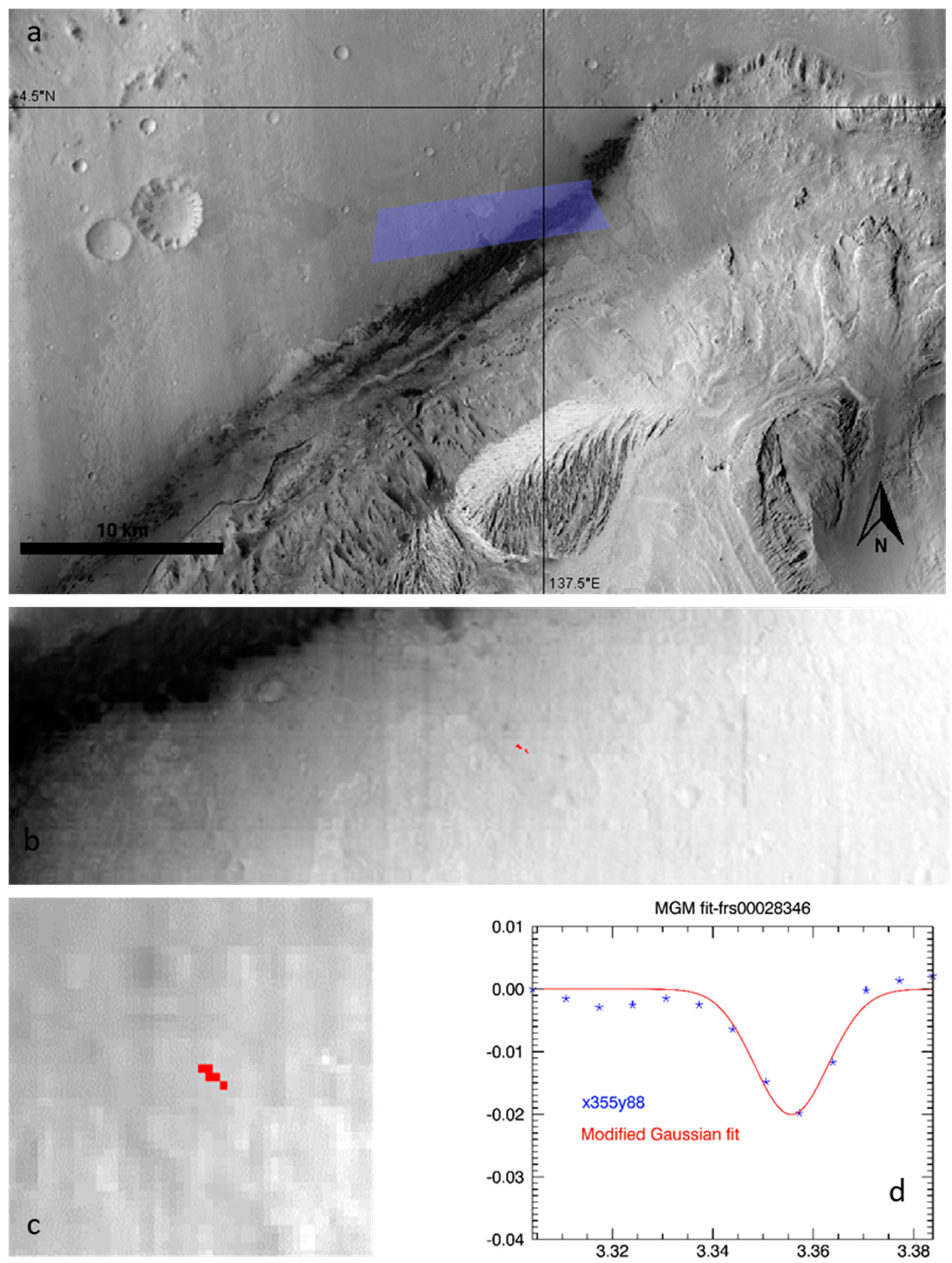
| Gale Crater | frs00028346 | 13 January 2013 | 243.7 |
| frt0000a091 | 20 February 2008 | 34.5 | |
| frt0001968 | 21 June 2010 | 107.4 | |
| hrs0000336a | 30 November 2006 | 143.2 | |
| Oxia Planum | frs0003a896 | 23 February 2016 | 112.8 |
| frs00031523 | 21 July 2014 | 165.1 | |
| frt00010fe9 | 11 February 2009 | 208 | |
| atu0004180 | 5 February 2017 | 312 | |
| hrl0000a3de | 4 March 2008 | 40.3 | |
| hrs00011725 | 5 March 2009 | 221.2 | |
| Nili Fossae | frs00041a28 | 14 February 2017 | 317.2 |
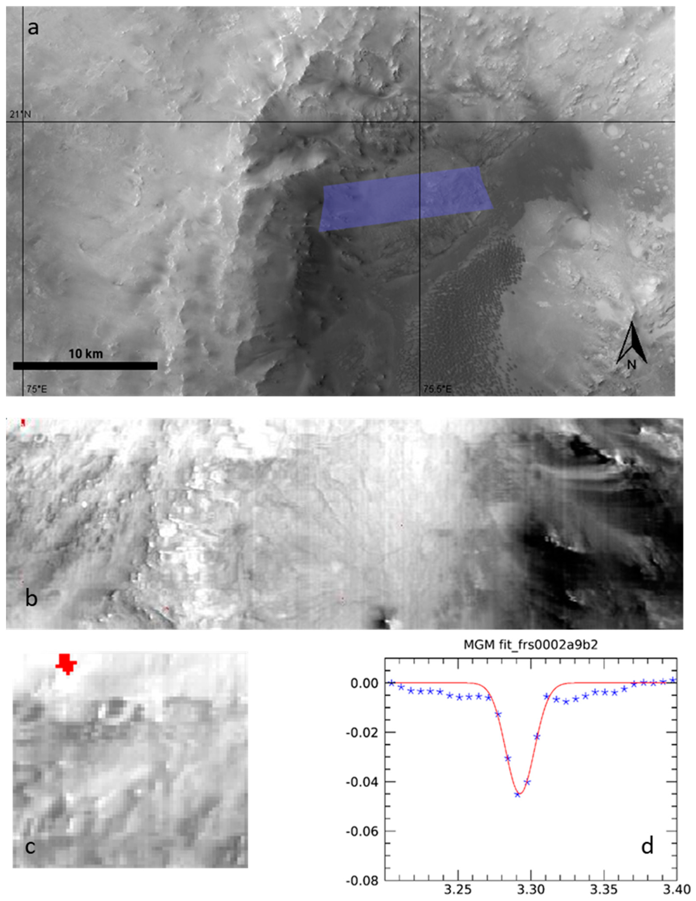
| frs0002a9b2 | 30 July 2013 | 359.6 | |
| frs0002adc4 | 16 August 2013 | 7.7 | |
| frs00039936 | 23 December 2015 | 85.2 |
| Area | CRISM-MRO Observation | Coordinate of the Deepest Pixel in the Cluster | Band Center | Depth | Number of Pixels in the Cluster | μc σc Depth of the Cluster |
|---|---|---|---|---|---|---|
| Gale Crater | frs00028346 | x355y88 | 3.35 | 0.022 | 5 | 0.009, 0.007 |
| frt0000a091 | - | - | - | - | - | |
| frt00001968 | x121y106 | 3.35 | 0.057 | 5 | 0.05, 0.007 | |
| hrs0000336a | - | - | - | - | - | |
| Oxia Planum | frs0003a896 | x420y133 | 3.29 | 0.024 | 6 | 0.002, 0.005 |
| frs00031523 | x459y165 | 3.32 | 0.040 | 7 | 0.03, 0.013 | |
| frt00010fe9 | x120y139 | 3.31 | 0.032 | 5 | 0.03, 0.007 | |
| atu0004180 | x345y172 | 3.28 | 0.036 | 8 | 0.03, 0.007 | |
| hrl0000a3de | - | - | - | - | ||
| hrs00011725 | x182y8 | 3.29 | 0.023 | 5 | 0.17, 0.003 | |
| Nili Fossae | frs00041a28 | x506y22 | 3.37 | 0.042 | 6 | 0.03, 0.007 |
| frs0002a9b2 | x47y3 | 3.29 | 0.045 | 15 | 0.044, 0.005 | |
| frs0002adc4 | - | - | - | - | ||
| frs00039936 | x135y49 | 3.29 | 0.014 | 4 | 0.013, 0.0005 |
| Area | CRISM-MRO Observation | Number of Pixels in Depth Map | Standard Deviation on Depth Map (σ) | Average (μ) | Threshold μ + 5σ |
|---|---|---|---|---|---|
| Gale Crater | frs00028346 | 84,475 | 0.003 | 0.0055 | 0.0205 |
| frt0000a091 | 228,660 | 0.003 | 0.005 | 0.02 | |
| frt00001968 | 221,400 | 0.004 | 0.007 | 0.027 | |
| hrs0000336a | 51,940 | 0.002 | 0.01 | 0.02 | |
| Oxia Planum | frs0003a896 | 83,550 | 0.002 | 0.005 | 0.015 |
| frs00031523 | 73,920 | 0.003 | 0.004 | 0.019 | |
| frt00010fe9 | 228,900 | 0.003 | 0.006 | 0.021 | |
| atu0004180 | 91,575 | 0.003 | 0.003 | 0.018 | |
| hrl0000a3de | 112,518 | 0.004 | 0.0037 | 0.0237 | |
| hrs00011725 | 51,900 | 0.002 | 0.005 | 0.015 | |
| Nili Fossae | frs00041a28 | 82,500 | 0.003 | 0.0036 | 0.0186 |
| frs0002a9b2 | 90,234 | 0.002 | 0.004 | 0.014 | |
| frs0002adc4 | 87,920 | 0.002 | 0.0036 | 0.0136 | |
| frs00039936 | 79,750 | 0.002 | 0.004 | 0.014 |
| Area | CRISM-MRO Observation | Threshold μ + 5σ | Lower Limit of Concentrations |
|---|---|---|---|
| Gale Crater | frs00028346 | 0.0205 | 300 |
| frt0000a091 | 0.02 | 350 | |
| frt00001968 | 0.027 | 600 | |
| hrs0000336a | 0.02 | 400 | |
| Oxia Planum | frs0003a896 | 0.015 | 220 |
| frs00031523 | 0.019 | 350 | |
| frt00010fe9 | 0.021 | 300 | |
| atu0004180 | 0.018 | 280 | |
| hrl0000a3de | 0.0237 | 320 | |
| hrs00011725 | 0.015 | 200 | |
| Nili Fossae | frs00041a28 | 0.0186 | 180 |
| frs0002a9b2 | 0.014 | 210 | |
| frs0002adc4 | 0.0136 | 200 | |
| frs00039936 | 0.014 | 200 |
Publisher’s Note: MDPI stays neutral with regard to jurisdictional claims in published maps and institutional affiliations. |
© 2022 by the authors. Licensee MDPI, Basel, Switzerland. This article is an open access article distributed under the terms and conditions of the Creative Commons Attribution (CC BY) license (https://creativecommons.org/licenses/by/4.0/).
Share and Cite
Manzari, P.; Marzo, C.; Ammannito, E. Investigation of Absorption Bands around 3.3 μm in CRISM Data. Remote Sens. 2022, 14, 5028. https://doi.org/10.3390/rs14195028
Manzari P, Marzo C, Ammannito E. Investigation of Absorption Bands around 3.3 μm in CRISM Data. Remote Sensing. 2022; 14(19):5028. https://doi.org/10.3390/rs14195028
Chicago/Turabian StyleManzari, Paola, Cosimo Marzo, and Eleonora Ammannito. 2022. "Investigation of Absorption Bands around 3.3 μm in CRISM Data" Remote Sensing 14, no. 19: 5028. https://doi.org/10.3390/rs14195028