
Multi-Sensor Remote Sensing of Intertidal Flat Habitats for Migratory Shorebird Conservation
 , and
, and
Abstract
:
1. Introduction
- (1)
- How well can a combination of multispectral reflectance and SAR backscatter and spectral unmixing techniques as implemented in Google Earth Engine be used to discriminate between mud and sand intertidal types?
- (2)
- Is the relationship between multispectral reflectance, SAR backscatter, and sediment type applicable across two very different geographic locations?
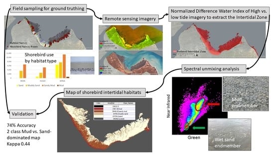
2. Methods
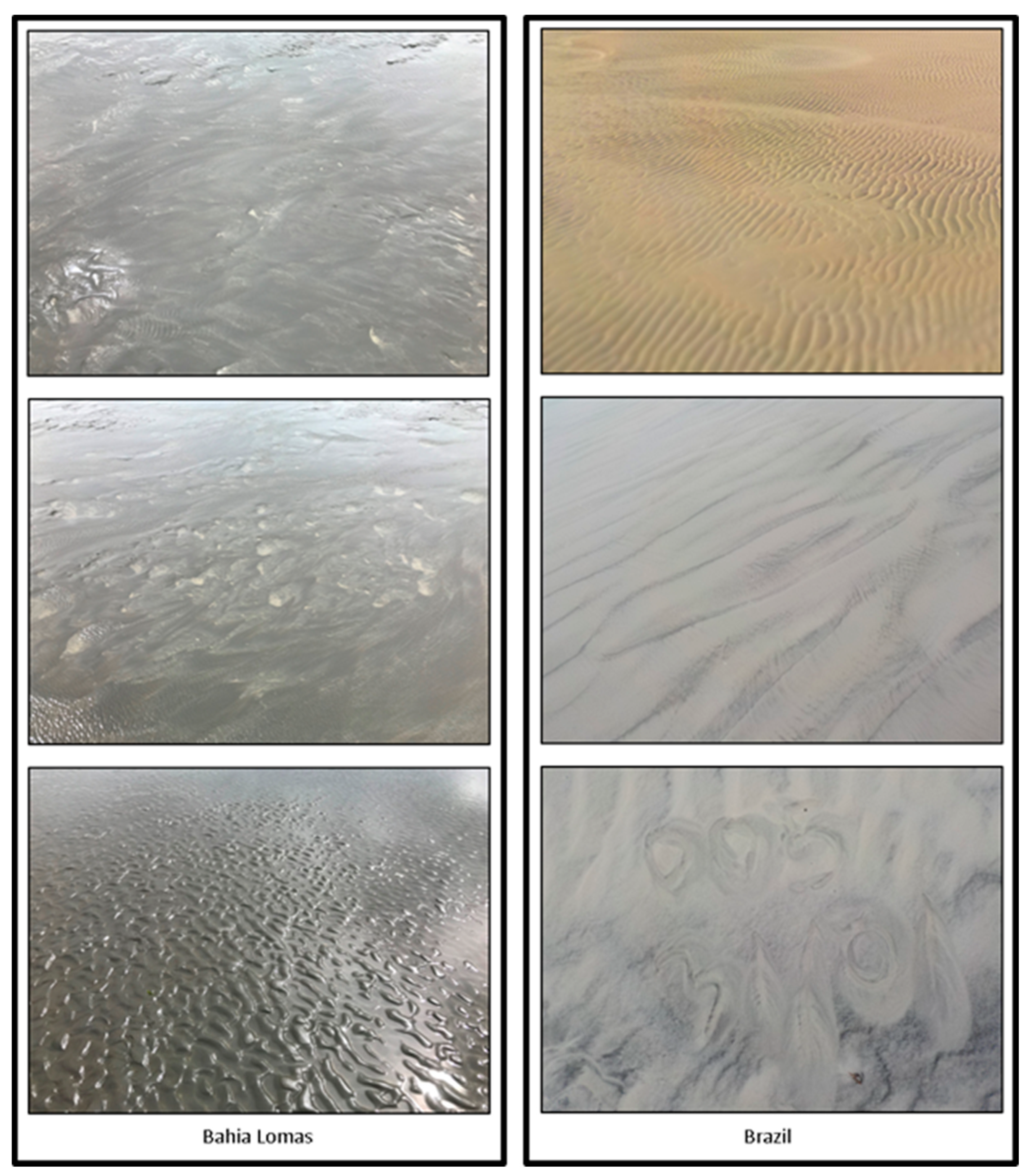
2.1. Study Sites
2.2. Field Data Collection
2.3. Landsat Reflectance Data Acquisition/Preparation
2.4. Sentinel-1 SAR Data Acquisition/Preparation
2.5. Intertidal Mask
2.6. Spectral Pattern Analysis
2.7. Unmixing Analysis and Classification
3. Results
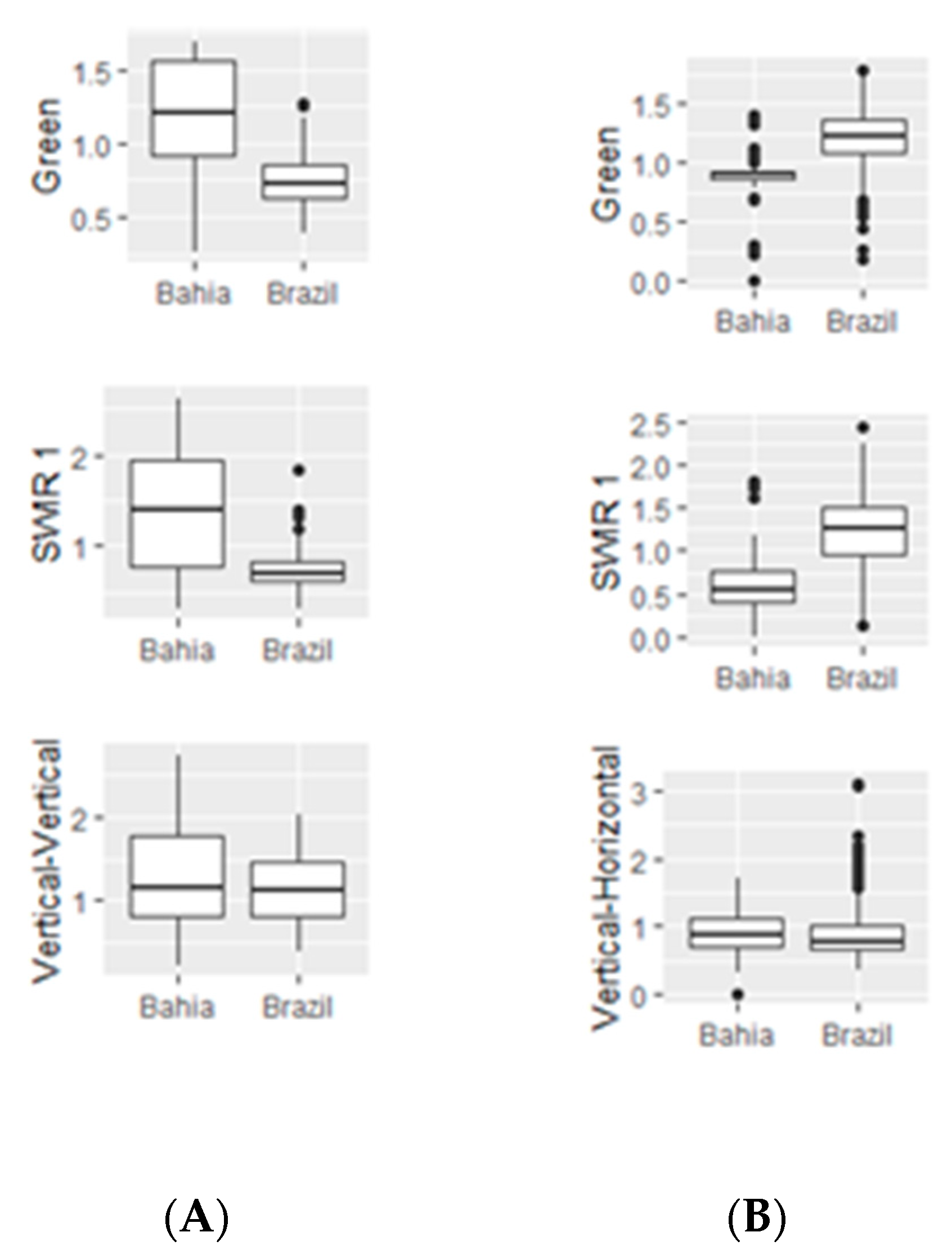
3.1. Spectral Pattern Analysis
3.2. Spectral Unmixing and Classification
3.3. Habitat Characterization
4. Discussion
5. Conclusions
Author Contributions
Funding
Data Availability Statement
Acknowledgments
Conflicts of Interest
Appendix A

References
- Colwell, M.A. Shorebird Ecology, Conservation, and Management; University of California Press: Berkeley, CA, USA, 2010. [Google Scholar]
- Niles, L.J.; Sitters, H.P.; Dey, A.D.; Atkinson, P.W.; Baker, A.J.; Bennett, K.A.; Carmona, R.C.; Clark, K.E.; Clark, N.A.; Espoz, C.; et al. Status of the Red Knot (Calidris canutus rufa) in the Western Hemisphere. In Studies in Avian Biology; Cooper Ornithological Society: Los Angeles, CA, USA, 2008. [Google Scholar]
- Burger, J.; Niles, L.J.; Porter, R.R.; Dey, A.D.; Koch, S.L.; Gordon, C. Migration and Over-Wintering of Red Knots (Calidris canutus rufa) along the Atlantic Coast of the United States. Ornithol. Appl. 2012, 114, 302–313. [Google Scholar] [CrossRef]
- Gratto-Trevor, C.; Morrison, R.I.G.; Mizrahi, D.; Lank, D.B.; Hicklin, P.; Spaans, A.L. Migratory Connectivity of Semi-palmated Sandpipers: Winter Distribution and Migration Routes of Breeding Populations. Waterbirds 2012, 35, 83–95. [Google Scholar] [CrossRef]
- Lathrop, R.G.; Niles, L.; Smith, P.; Peck, M.; Dey, A.; Sacatelli, R.; Bognar, J. Mapping and modeling the breeding habitat of the Western Atlantic Red Knot (Calidris canutus rufa) at local and regional scales. Ornithol. Appl. 2018, 120, 650–665. [Google Scholar] [CrossRef] [Green Version]
- Warnock, N. Stopping vs. staging: The difference between a hop and a jump. J. Avian Biology 2010, 4, 621–626. [Google Scholar] [CrossRef]
- Brown, S.; Gratto-Trevor, C.; Porter, R.; Weiser, E.; Mizrahi, D.; Bentzen, R.; Boldenow, M.; Clay, R.; Freeman, S.; Giroux, M.-A.; et al. Migratory connectivity of Semipalmated Sandpipers and implications for conservation. Ornithol. Appl. 2017, 119, 207–224. [Google Scholar] [CrossRef] [Green Version]
- Anderson, A.M.; Duijns, S.; Smith, P.A.; Friis, C.; Nol, E. Migration Distance and Body Condition Influence Shorebird Migration Strategies and Stopover Decisions During Southbound Migration. Front. Ecol. Evol. 2019, 7, 251. [Google Scholar] [CrossRef] [Green Version]
- Burger, J.; Niles, L.; Clark, K.E. Importance of beach, mudflat and marsh habitats to migrant shorebirds on Delaware Bay. Biol. Conserv. 1997, 79, 283–292. [Google Scholar] [CrossRef]
- Mu, T.; Wilcove, D.S. Upper tidal flats are disproportionately important for the conservation of migratory shorebirds. Proc. R. Soc. B Boil. Sci. 2020, 287, 20200278. [Google Scholar] [CrossRef]
- Jourdan, C.; Fort, J.; Pinaud, D.; Delaporte, P.; Gernigon, J.; Lachaussée, N.; Lemesle, J.-C.; Pignon-Mussaud, C.; Pineau, P.; Robin, F.; et al. Nycthemeral Movements of Wintering Shorebirds Reveal Important Differences in Habitat Uses of Feeding Areas and Roosts. Estuaries Coasts 2021, 44, 1454–1468. [Google Scholar] [CrossRef]
- Colwell, M.A.; Landrum, S.L. Nonrandom Shorebird Distribution and Fine-Scale Variation in Prey Abundance. Ornithol. Appl. 1993, 95, 94–103. [Google Scholar] [CrossRef]
- Erwin, R.M. Dependence of Waterbirds and Shorebirds on Shallow-Water Habitats in the Mid-Atlantic Coastal Region: An Ecological Profile and Management Recommendations. Estuaries 1996, 19, 213–219. [Google Scholar] [CrossRef]
- Thrush, S.; Hewitt, J.; Norkko, A.; Nicholls, P.; Funnell, G.; Ellis, J. Habitat change in estuaries: Predicting broad-scale responses of intertidal macrofauna to sediment mud content. Mar. Ecol. Prog. Ser. 2003, 263, 101–112. [Google Scholar] [CrossRef] [Green Version]
- Van der Wal, D.; Herman, P.M.J.; Forster, R.; Ysebaert, T.; Rossi, F.; Knaeps, E.; Plancke, Y.; Ides, S. Distribution and dynamics of intertidal macrobenthos predicted from remote sensing: Response to microphytobenthos and environment. Mar. Ecol. Prog. Ser. 2008, 367, 57–72. [Google Scholar] [CrossRef]
- Cozzoli, F.; Bouma, T.; Ysebaert, T.; Herman, A. Application of non-linear quantile regression to macrozoobenthic species distribution modelling: Comparing two contrasting basins. Mar. Ecol. Prog. Ser. 2013, 475, 119–133. [Google Scholar] [CrossRef]
- Sheaves, M.; Dingle, L.; Mattone, C. Biotic hotspots in mangrove-dominated estuaries: Macro-invertebrate aggregation in unvegetated lower intertidal flats. Mar. Ecol. Prog. Ser. 2016, 556, 31–43. [Google Scholar] [CrossRef] [Green Version]
- Bocher, P.; Robin, F.; Kojadinovic, J.; Delaporte, P.; Rousseau, P.; Dupuy, C.; Bustamante, P. Trophic resource partitioning within a shorebird community feeding on intertidal mudflat habitats. J. Sea Res. 2014, 92, 115–124. [Google Scholar] [CrossRef] [Green Version]
- Philippe, A.S.; Pinaud, D.; Cayatte, M.-L.; Goulevant, C.; Lachaussée, N.; Pineau, P.; Karpytchev, M.; Bocher, P. Influence of environmental gradients on the distribution of benthic resources available for shorebirds on intertidal mudflats of Yves Bay, France. Estuar. Coast. Shelf Sci. 2016, 174, 71–81. [Google Scholar] [CrossRef]
- Faria, F.A.; Albertoni, E.F.; Bugoni, L. Trophic niches and feeding relationships of shorebirds in southern Brazil. Aquat. Ecol. 2018, 52, 281–296. [Google Scholar] [CrossRef]
- Burger, J.; Niles, L.; Jeitner, C.; Gochfeld, M. Habitat risk: Use of intertidal flats by foraging red knots (Calidris canutus rufa), ruddy turnstones, (Arenaria interpres), semipalmated sandpipers (Calidris pusilla), and sanderling (Calidris alba) on Delaware Bay beaches. Environ. Res. 2018, 165, 237–246. [Google Scholar] [CrossRef]
- Galbraith, H.; Jones, R.; Park, R.; Clough, J.; Herrod-Julius, S.; Harrington, B.; Page, G. Global Climate Change and Sea Level Rise: Potential Losses of Intertidal Habitat for Shorebirds. Waterbirds 2002, 25, 173–183. [Google Scholar] [CrossRef]
- Iwamura, T.; Possingham, H.; Chadès, I.; Minton, C.; Murray, N.; Rogers, D.I.; Treml, E.; Fuller, R. Migratory connectivity magnifies the consequences of habitat loss from sea-level rise for shorebird populations. Proc. R. Soc. B Boil. Sci. 2013, 280, 20130325. [Google Scholar] [CrossRef] [Green Version]
- Galbraith, H.; DesRochers, D.W.; Brown, S.; Reed, J.M. Predicting Vulnerabilities of North American Shorebirds to Climate Change. PLoS ONE 2014, 9, e108899. [Google Scholar] [CrossRef] [Green Version]
- Piersma, T.; Lindström, Å. Migrating shorebirds as integrative sentinels of global environmental change. IBIS 2004, 146, 61–69. [Google Scholar] [CrossRef]
- Studds, C.E.; Kendall, B.E.; Murray, N.J.; Wilson, H.B.; Rogers, D.I.; Clemens, R.S.; Gosbell, K.; Hassell, C.J.; Jessop, R.; Melville, D.S.; et al. Rapid population decline in migratory shorebirds relying on Yellow Sea tidal mudflats as stopover sites. Nat. Commun. 2017, 8, 14895. [Google Scholar] [CrossRef] [Green Version]
- Murray, N.J.; Phinn, S.R.; DeWitt, M.; Ferrari, R.; Johnston, R.; Lyons, M.B.; Clinton, N.; Thau, D.; Fuller, R.A. The global distribution and trajectory of tidal flats. Nature 2018, 565, 222–225. [Google Scholar] [CrossRef]
- Murray, N.J.; Phinn, S.R.; Clemens, R.S.; Roelfsema, C.M.; Fuller, R.A. Continental Scale Mapping of Tidal Flats across East Asia Using the Landsat Archive. Remote Sens. 2012, 4, 3417–3426. [Google Scholar] [CrossRef] [Green Version]
- Murray, N.J.; Clemens, R.S.; Phinn, S.R.; Possingham, H.P.; Fuller, R.A. Tracking the rapid loss of tidal wetlands in the Yellow Sea. Front. Ecol. Environ. 2014, 12, 267–272. [Google Scholar] [CrossRef] [Green Version]
- Murray, N.J.; Ma, Z.; Fuller, R.A. Tidal flats of the Yellow Sea: A review of ecosystem status and anthropogenic threats: Status of Yellow Sea tidal flats. Austral Ecol. 2015, 40, 472–481. [Google Scholar] [CrossRef] [Green Version]
- Gorelick, N.; Hancher, M.; Dixon, M.; Ilyushchenko, S.; Thau, D.; Moore, R. Google Earth Engine: Planetary-scale geospatial analysis for everyone. Remote Sens. Environ. 2017, 202, 18–27. [Google Scholar] [CrossRef]
- Zhang, K.; Dong, X.; Liu, Z.; Gao, W.; Hu, Z.; Wu, G. Mapping Tidal Flats with Landsat 8 Images and Google Earth Engine: A Case Study of the China’s Eastern Coastal Zone circa 2015. Remote Sens. 2019, 11, 924. [Google Scholar] [CrossRef]
- Chang, M.; Li, P.; Li, Z.; Wang, H. Mapping Tidal Flats of the Bohai and Yellow Seas Using Time Series Sentinel-2 Images and Google Earth Engine. Remote Sens. 2022, 14, 1789. [Google Scholar] [CrossRef]
- Rainey, M.; Tyler, A.; Gilvear, D.; Bryant, R.; McDonald, P. Mapping intertidal estuarine sediment grain size distributions through airborne remote sensing. Remote Sens. Environ. 2003, 86, 480–490. [Google Scholar] [CrossRef]
- Yates, M.G.; Jones, A.R.; McGrorty, S.; Goss-Custard, J.D. The Use of Satellite Imagery to Determine the Distribution of Intertidal Surface Sediments of The Wash, England. Estuar. Coast. Shelf Sci. 1993, 36, 333–344. [Google Scholar] [CrossRef]
- Ryu, J.-H.; Na, Y.-H.; Won, J.-S.; Doerffer, R. A critical grain size for Landsat ETM+ investigations into intertidal sediments: A case study of the Gomso tidal flats, Korea. Estuar. Coast. Shelf Sci. 2004, 60, 491–502. [Google Scholar] [CrossRef]
- Van der Wal, D.; Herman, P.M.J. Regression-based synergy of optical, shortwave infrared and microwave remote sensing for monitoring the grain-size of intertidal sediments. Remote Sens. Environ. 2007, 111, 89–106. [Google Scholar] [CrossRef]
- Gao, C.; Xu, M.; Xu, H.; Zhou, W. Retrieving Photometric Properties and Soil Moisture Content of Tidal Flats Using Bidirectional Spectral Reflectance. Remote Sens. 2021, 13, 1402. [Google Scholar] [CrossRef]
- Choi, J.-K.; Ryu, J.-H.; Lee, Y.-K.; Yoo, H.-R.; Woo, H.J.; Kim, C.H. Quantitative estimation of intertidal sediment characteristics using remote sensing and GIS. Estuar. Coast. Shelf Sci. 2010, 88, 125–134. [Google Scholar] [CrossRef]
- Rainey, M.P.; Tyler, A.N.; Bryant, R.G.; Gilvear, D.J.; McDonald, P. The influence of surface and interstitial moisture on the spectral characteristics of intertidal sediments: Implications for airborne image acquisition and processing. Int. J. Remote Sens. 2000, 21, 3025–3038. [Google Scholar] [CrossRef]
- Baghdadi, N.; Cerdan, O.; Zribi, M.; Auzet, V.; Darboux, F.; El Hajj, M.; Kheir, R.B. Operational performance of current synthetic aperture radar sensors in mapping soil surface characteristics in agricultural environments: Application to hydrological and erosion modelling. Hydrol. Process. 2007, 22, 9–20. [Google Scholar] [CrossRef]
- Anderson, K.; Croft, H. Remote sensing of soil surface properties. Prog. Phys. Geogr. Earth Environ. 2009, 33, 457–473. [Google Scholar] [CrossRef]
- Van der Wal, D.; Herman, P.M.J.; Wielemaker-van den Dool, A. Characterisation of surface roughness and sediment texture of intertidal flats using ERS SAR imagery. Remote Sens. Environ. 2005, 98, 96–109. [Google Scholar] [CrossRef]
- Gade, M.; Melchionna, S.; Stelzer, K.; Kohlus, J. Multi-frequency SAR data help improving the monitoring of intertidal flats on the German North Sea coast. Estuar. Coast. Shelf Sci. 2014, 140, 32–42. [Google Scholar] [CrossRef]
- Adolph, W.; Farke, H.; Lehner, S.; Ehlers, M. Remote Sensing Intertidal Flats with TerraSAR-X. A SAR Perspective of the Structural Elements of a Tidal Basin for Monitoring the Wadden Sea. Remote Sens. 2018, 10, 1085. [Google Scholar] [CrossRef] [Green Version]
- De Moura, R.L.; Minte-Vera, C.V.; Curado, I.B.; Francini-Filho, R.B.; Rodrigues, H.D.C.L.; Dutra, G.F.; Alves, D.C.; Souto, F.J.B. Challenges and Prospects of Fisheries 127 Co-Management under a Marine Extractive Reserve Framework in North-eastern Brazil. Coast. Manag. 2009, 37, 617–632. [Google Scholar] [CrossRef]
- Santos, C.Z.; Schiavetti, A. Assessment of the management in Brazilian Marine Extractive Reserves. Ocean Coast. Manag. 2014, 93, 26–36. [Google Scholar] [CrossRef]
- Kober, K.; Bairlein, F. Habitat Choice and Niche Characteristics Under Poor Food Conditions. A Study on Migratory Nearctic Shorebirds in the Intertidal Flats of Brazil. Ardea 2009, 97, 31–42. [Google Scholar] [CrossRef]
- Morrison, R.I.G.; Ross, R.K. Atlas of Nearctic Shorebirds on the Coast of South America; Special Publication, Canadian Wildlife Service: Ottawa, ON, Canada, 1989; Volume 2. [Google Scholar]
- Folk, R.L. The Distinction between Grain Size and Mineral Composition in Sedimentary-Rock Nomenclature. J. Geol. 1954, 62, 344–359. [Google Scholar] [CrossRef]
- Thien, S.J. A flow diagram for teaching texture-by-feel analysis. J. Agron. Educ. 1979, 8, 54–55. [Google Scholar] [CrossRef]
- Martinuzzi, S.; Gould, W.A.; Ramos Gonzalez, O.M. Creating Cloud-Free Landsat ETM+ Data Sets. In Tropical Land-Scapes: Cloud and Cloud-Shadow Removal; U.S. Department of Agriculture, Forest Service, International Institute of Tropical Forestry: San Juan, PR, USA, 2007. [Google Scholar]
- Egbert, G.D.; Erofeeva, S.Y. Efficient Inverse Modeling of Barotropic Ocean Tides. J. Atmos. Ocean. Technol. 2002, 19, 183–204. [Google Scholar] [CrossRef]
- Jensen, J.R. Remote Sensing of the Environment: An Earth Resource Perspective, 2nd ed.; Pearson Prentice Hall: Upper Saddle River, NJ, USA, 2007. [Google Scholar]
- Settle, J.J.; Drake, N.A. Linear mixing and the estimation of ground cover proportions. Int. J. Remote Sens. 1993, 14, 1159–1177. [Google Scholar] [CrossRef]
- Espoz, C.; Ponce, A.; Matus, R.; Blank, O.; Rozbaczylo, N.; Sitters, H.P.; Rodriguez, S.; Dey, A.D.; Niles, L.J. Trophic ecology of the Red Knot Calidris canutus rufa at Bahía Lomas, Tierra del Fuego, Chile. Wader Study Group Bull 2008, 115, 69–76. [Google Scholar]
- Henriques, M.; Catry, T.; Belo, J.R.; Piersma, T.; Pontes, S.; Granadeiro, J.P. Combining Multispectral and Radar Imagery with Machine Learning Techniques to Map Intertidal Habitats for Migratory Shorebirds. Remote Sens. 2022, 14, 3260. [Google Scholar] [CrossRef]
- Kumar, L.; Mutanga, O. Google Earth Engine Applications Since Inception: Usage, Trends, and Potential. Remote Sens. 2018, 10, 1509. [Google Scholar] [CrossRef] [Green Version]
- Merchant, D. Modeling, and Management of Migratory Shorebird Habitat in Northern Brazil using Remote Sensing. PhD Thesis, Rutgers University, New Brunswick, NJ, USA, 2021. [Google Scholar] [CrossRef]
- Essink, K. Ecological effects of dumping of dredged sediments; options for management. J. Coast. Conserv. 1999, 5, 69–80. [Google Scholar] [CrossRef]
- Peterson, C.H.; Bishop, M.J.; Johnson, G.A.; D’Anna, L.M.; Manning, L.M. Exploiting beach filling as an unaffordable experiment: Benthic intertidal impacts propagating upwards to shorebirds. J. Exp. Mar. Biol. Ecol. 2006, 338, 205–221. [Google Scholar] [CrossRef]
- Jaffe, B.E.; Smith, R.E.; Foxgrover, A.C. Anthropogenic influence on sedimentation and intertidal mudflat change in San Pablo Bay, California: 1856–1983. Estuar. Coast. Shelf Sci. 2007, 73, 175–187. [Google Scholar] [CrossRef]
- Van Maren, D.S.; van Kessel, T.; Cronin, K.; Sittoni, L. The impact of channel deepening and dredging on estuarine sediment concentration. Cont. Shelf Res. 2015, 95, 1–14. [Google Scholar] [CrossRef]


| Band | Normalized Sand | Normalized Mud | |
|---|---|---|---|
| Landsat 8 | Blue | <0.001 | <0.001 |
| Green | <0.001 | <0.001 | |
| Red | <0.001 | <0.001 | |
| Near IR | <0.001 | <0.001 | |
| SWIR 1 | <0.001 | <0.001 | |
| SWIR 2 | <0.001 | <0.001 | |
| Sentinel-1 | Vertical-Vertical | 0.553 | 0.082 |
| Vertical-Horizontal | 0.011 | 0.638 |
| (A) 3 Class Sand-Mixed-Mud Map (n = 475). | ||||||
|---|---|---|---|---|---|---|
| Reference | ||||||
| Mud | Mixed | Sand | Sum | User’s | ||
| Classified | Mud | 86 | 27 | 68 | 181 | 48% |
| Mixed | 8 | 9 | 76 | 93 | 10% | |
| Sand | 9 | 7 | 185 | 201 | 92% | |
| Sum | 103 | 43 | 329 | 475 | ||
| Producer’s | 83% | 21% | 56% | Overall | 59% | |
| Kappa | 0.33 | |||||
| (B) 2 Class Sand vs. Mud-Dominated Map (n =232). | ||||||
| Reference | ||||||
| Mud | Sand | Sum | User’s | |||
| Classified | Mud | 60 | 58 | 118 | 51% | |
| Sand | 3 | 111 | 114 | 97% | ||
| Sum | 63 | 169 | 232 | |||
| Producer’s | 95% | 66% | Overall | 74% | ||
| Kappa | 0.48 | |||||
| (A) 4 Class Sand-Mixed-Mud Map | ||||||
|---|---|---|---|---|---|---|
| Reference | ||||||
| Classified | Mud | Sandy Mud | Muddy Sand | Sand | Sum | User’s |
| Mud | 5 | 3 | 2 | 0 | 10 | 50% |
| Sandy Mud | 18 | 7 | 6 | 1 | 32 | 22% |
| Muddy Sand | 3 | 10 | 16 | 3 | 32 | 50% |
| Sand | 2 | 19 | 28 | 51 | 100 | 51% |
| Sum | 28 | 39 | 52 | 55 | 174 | |
| Producer’s | 18% | 18% | 31% | 93% | Overall | 45% |
| Kappa | 0.23 | |||||
| (B) 2 Class Sand vs. Mud-Dominated Map | ||||||
| Reference | ||||||
| Mud | Sand | Sum | User’s | |||
| Classified | Mud | 33 | 9 | 42 | 78% | |
| Sand | 34 | 98 | 132 | 74% | ||
| Sum | 67 | 107 | ||||
| Producer’s | 49% | 92% | Overall | 75% | ||
| Kappa | 0.44 | |||||
| Intertidal Sediment Type | Area Inside MER | Area Outside MER | Area Total | |||||
|---|---|---|---|---|---|---|---|---|
| Ha | % of MER | % of Total | Ha | % of Out | % of Total | Ha | % of Total | |
| Mud | 21,944 | 50.0% | 19.5 | 32,686 | 47.5% | 29.0% | 54,630 | 48.5% |
| Mixed | 10,658 | 24.3% | 9.5 | 21,720 | 31.5% | 19.3% | 32,378 | 28.7% |
| Sand | 11,253 | 25.7% | 10.0 | 14,455 | 21.0% | 12.8% | 25,708 | 22.8% |
| Total | 43,855 | 38.9% | 68,861 | 61.1% | 112,716 | |||
| Intertidal Sediment Type | Area (ha) | Area (%) |
|---|---|---|
| Mud | 1664 | 5.4% |
| Sandy Mud | 6129 | 20.0% |
| Muddy Sand | 6740 | 22.0% |
| Sand | 16,110 | 52.6% |
Publisher’s Note: MDPI stays neutral with regard to jurisdictional claims in published maps and institutional affiliations. |
© 2022 by the authors. Licensee MDPI, Basel, Switzerland. This article is an open access article distributed under the terms and conditions of the Creative Commons Attribution (CC BY) license (https://creativecommons.org/licenses/by/4.0/).
Share and Cite
Lathrop, R.G.; Merchant, D.; Niles, L.; Paludo, D.; Santos, C.D.; Larrain, C.E.; Feigin, S.; Smith, J.; Dey, A. Multi-Sensor Remote Sensing of Intertidal Flat Habitats for Migratory Shorebird Conservation. Remote Sens. 2022, 14, 5016. https://doi.org/10.3390/rs14195016
Lathrop RG, Merchant D, Niles L, Paludo D, Santos CD, Larrain CE, Feigin S, Smith J, Dey A. Multi-Sensor Remote Sensing of Intertidal Flat Habitats for Migratory Shorebird Conservation. Remote Sensing. 2022; 14(19):5016. https://doi.org/10.3390/rs14195016
Chicago/Turabian StyleLathrop, Richard G., Daniel Merchant, Larry Niles, Danielle Paludo, Carlos David Santos, Carmen Espoz Larrain, Stephanie Feigin, Joseph Smith, and Amanda Dey. 2022. "Multi-Sensor Remote Sensing of Intertidal Flat Habitats for Migratory Shorebird Conservation" Remote Sensing 14, no. 19: 5016. https://doi.org/10.3390/rs14195016