Optimized Software Tools to Generate Large Spatio-Temporal Data Using the Datacubes Concept: Application to Crop Classification in Cap Bon, Tunisia

Abstract

In the context of a changing climate, monitoring agricultural systems is becoming increasingly important. Remote sensing products provide essential information for the crop classification application, which is used to produce thematic maps. High-resolution and regional-scale maps of agricultural land are required to develop better adapted future strategies. Nevertheless, the performance of crop classification using large spatio-temporal data remains challenging due to the difficulties in handling huge amounts of input data (different spatial and temporal resolutions). This paper proposes an innovative approach of remote sensing data management that was used to prepare the input data for the crop classification application. This classification was carried out in the Cap Bon region, Tunisia, to classify citrus groves among two other crop classes (olive groves and open field) using multi-temporal remote sensing data from Sentinel- 1 and Sentinel-2 satellite platforms. Thus, we described the new QGIS plugin “Model Management Tool (MMT)”. This plugin was designed to manage large Earth observation (EO) data. This tool is based on the combination of two concepts: (i) the local nested grid (LNG) called Tuplekeys and (ii) Datacubes. Tuplekeys or special spatial regions were created within a LNG to allow a proper integration between the data of both sensors. The Datacubes concept allows to provide an arranged array of time-series multi-dimensional stacks (space, time and data) of gridded data. Two different classification processes were performed based on the selection of the input feature (the obtained time-series as input data: NDVI and NDVI + VV + VH) and on the most accurate algorithm for each scenario (22 tested classifiers). The obtained results revealed that the best classification performance and highest accuracy were obtained with the scenario using only optical-based information (NDVI), with an overall accuracy OA = 0.76. This result was obtained by support vector machine (SVM). As for the scenario relying on the combination of optical and SAR data (NDVI + VV + VH), it presented an OA = 0.58. Our results demonstrate the usefulness of the new data management tool in organizing the input classification data. Additionally, our results highlight the importance of optical data to provide acceptable classification performance especially for a complex landscape such as that of the Cap Bon. The information obtained from this work will allow the estimation of the water requirements of citrus orchards and the improvement of irrigation scheduling methodologies. Likewise, many future methodologies will certainly rely on the combination of Tuplekeys and Datacubes concepts which have been tested within the MMT tool.

1. Introduction

The citrus sub-sector is one of the main pillars of the Tunisian agricultural sector. The Cap Bon region is considered the main production area, with 75% of the total citrus area [1]. Given the socio-economic importance of the citrus sector in this region, monitoring the citrus orchards over time is crucial to ensure food supply and economic stability. Remote sensing provides data of great interest in the field of land cover and crop classification [2,3,4], especially given its capability to deliver regular spatial and temporal data over large areas. Citrus monitoring with remote sensing offers an operational method to support field inspection efforts [5]. The information obtained from this type of work is essential to perform more the rigorous control of water requirements, among many other applications, not only at the plot scale but also at the sub-regional and regional scale [6]. Indeed, the literature review showed that there are many studies analyzing crop classification over large areas using remote sensing information, which performs adequately when classifying winter, summer and spring crops, as well as when differentiating between open field and orchards [7,8,9]. Consequently, to establish the most effective management strategy, it is essential to periodically obtain precise remote sensing information [10,11].

Despite the socio-economic importance of the citrus sector in the Cap Bon region, it is not well reflected in the crop classification work conducted in the area. Indeed, according to the review of the literature on studies carried out in this region, we found a study conducted by [12] in Lebna, which is a watershed located in the Cap Bon area. This study aimed to explore the extent to which agricultural land fragmentation can influence farmers’ decisions regarding annual crop distribution by distinguishing and quantifying the influences of both crop sequences and adjacent crops. Another study was carried out in the Lebna region [13], whose aim was to examine the degree to which the spatio-temporal allocation of crops at the landscape scale is related to the rotations of collective crops. The study carried out by [14] was performed in the Haouaria plain and, according to the overall accuracy (OA) and kappa index (k), the classification of crop categories was relatively accurate, providing key information, such as the area of each crop type. However, we found no works studying the specific classification of trees and citrus groves, in particular, at the level of the entire Cap Bon region.

At a larger scale, the study conducted by [15] assessed citrus orchards in Florida using freely available Landsat ETM + satellite imagery combined with economic data collected by county to forecast citrus production. Recently, [16] employed a practical approach to follow citrus plantation dynamics using all the available Landsat records. This methodology incorporated a classification-based mask with time series change detection on the Google Earth Engine GEE platform. The application of this methodology successfully seized the dynamics of a 33-year-old citrus plantation in Xunwu County, China, involving the initial cultivation of the orchard during the period of constant extension (1986–2016), as well as the desertion of the orchard and its new cultivation. In addition, another citrus classification study was carried out in Florida by [5], with the main objective of assessing the effectiveness of using Sentinel-1A C-band Synthetic Aperture Radar (SAR) data to classify citrus fruits. Sentinel-1 C-band SAR data classification accuracies were observed to be slightly lower than cloudless free multi-temporal optical data (approximately 2.5% difference). However, the classification accuracy results were relatively similar, which suggested that Sentinel-1 SAR might be a useful imaging resource, particularly in regions with permanent cloud cover. In fact, SAR data have two main advantages over optical data. The first concerns the ability of SAR sensors to acquire data regardless of weather conditions and at night [17]. The second important property is the sensitivity of the SAR data to the canopy structure [18,19]. Therefore, the complementarity of optical and SAR data is hypothesized to offer information that can be particularly advantageous for crop classification applications [20].

Nevertheless, combining the use of multi-temporal optical and SAR data entails an extremely large amount of input information. This requires appropriate data organization, especially for a wide extension of the area. Additionally, combining the use of remote sensing images from different sensors, especially to perform time-series analysis (essential for precise crop classification tasks), involves dealing with many considerations such as different spectral, spatial resolution, etc. (explained in detail in [21]).

The new concept of Earth observation Datacubes (EODC) has recently shifted the way that users handle large spatio-temporal EO data [22,23]. It enhances interoperability between data, and enables data management for users [24]. EODC is an inventive methodology [25,26] allowing EO data to be gathered, organized, managed and explored. The objective of the Datacubes is to provide an arranged array of time-series multi-dimensional stacks (space, time and data) of “raster data” or “gridded data” [22,27,28]. Therefore, it simplifies applications based on dense time-series and even multi-sensor datasets, as well as concealing the difficulties for data users, who can then focus on the analysis instead of the data management [28].

The solution offered by the EODC approach can be complemented by the new and increasingly common solution of the local nested grid (LNG) [8,21,29]. The term “nested grid” is connected with the “tiling schema”, based on the “quad-tree” paradigm (explained in detail in [21]), which is a special spatial region designed automatically for the specific study area. These spatial regions have a grid structure, hence the term local nested grid, which is compatible with EO data. The concept of a “nested grid” was fully defined in [29].

This paper describes a classification approach for citrus groves among two other crop classes (olive groves and open field) located in the Cap Bon region. For this purpose, we suggest an innovative contribution in terms of software development and data management dedicated to the crop classification application. The “model management tool MMT”, presented in this study, is a QGIS plugin for large EO time series analysis. The authors designed this API considering (i) the management of input data through the combination of the spatial structuring of the LNG known as Tuplekeys and Datacubes to deal with large spatio-temporal EO data obtained from the different satellite sensors Sentinel-1 (SAR) and Sentinel-2 (optical); (ii) the procurement of the time series of NDVI, VV and VH corresponding to the training data from the Tuplekeys–Datacubes structure. This plugin allowed users to combine the use of different analysis-ready data (ARD) information employing a user-friendly interface and with minimal programming effort. Different machine learning algorithms (22 classifiers) and two scenarios (based on the selection of the obtained time-series as input data: NDVI and NDVI + VV + VH) were tested. Two different classification processes were performed based on the selection of input features (NDVI and NDVI + VV + VH) and on the most accurate algorithm corresponding to each scenario.

2. Materials and Methods

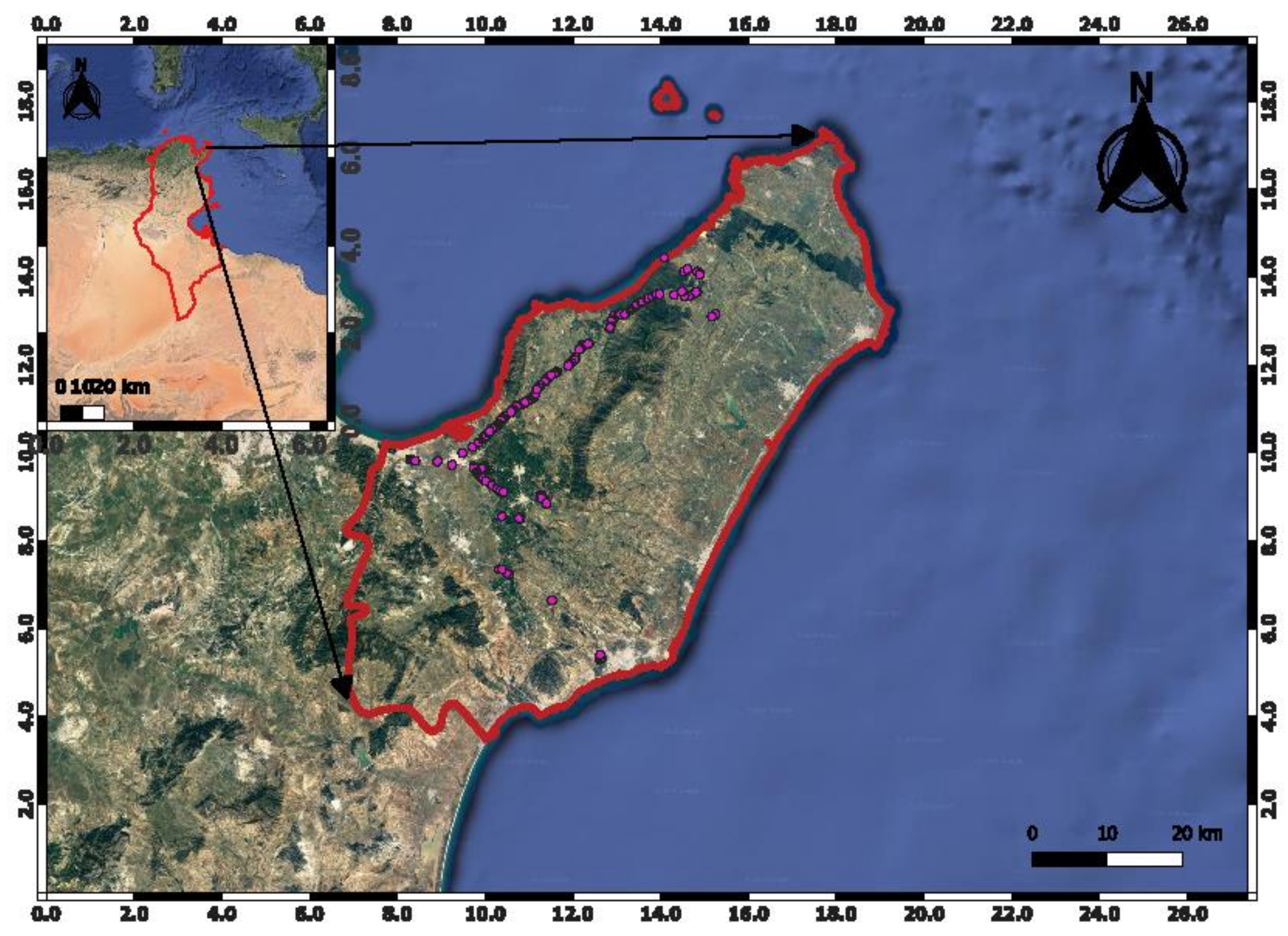
2.1. Study Area

This study was carried out on the scale of the entire Cap Bon region, Tunisia (Figure 1). The Cap Bon region covers 2825 km², or 2.4% of the country’s surface area [30]. Of this area, 199,344 ha is plowed land, of which more than 24% is irrigated. This region is considered an important agricultural hub [31], as the cultivated area accounts for 4% of the country’s cultivated area and contributes 15% of the value of national agricultural production. The climate varies from sub-humid to semi-arid, and the average annual amount of rain in the region varies between 390 and 630 mm. The study area is characterized by significant and variable evaporation in time. The estimated annual total annual evapotranspiration exceeds 1100 mm [32]. The dominant plant products are citrus, vines, spices and vegetables (mostly tomatoes and peppers).

2.2. Remote Sensing Data: Sentinel-1 and Sentinel-2 Dataset

The Google Earth Engine GEE, the new cloud solution, is currently receiving increasing attention as an innovative tool to search and download EO data in a way that was not previously possible (rapid access to large spatio-temporal data). We thus decided to use GEE, which provides analysis-ready data (ARD), to download the Sentinel-1 and Sentinel-2 datasets.

GEE is an IT platform that permits that users execute a geospatial analysis of Google’s infrastructure [33]. Datasets can be seen in the GEE Explorer and imported into the Code Editor. The GEE Data Catalog incorporates a variety of standard EO datasets, including data from large programs, such as Landsat and Copernicus. The GEE Code Editor is a web-based Integrated Development Environment IDE for writing and executing scripts in JavaScript. In this case study, the scripts were relatively straightforward, and we utilized only simple commands to download data for the period September 2020–June 2021:102 acquisition dates for VV and VH from Sentinel-1 and 43 acquisition dates for NDVI Sentinel-2 scenes.

2.3. Classification Methodology

The classification approach adopted can be considered a typical workflow using satellite image time series. In fact, we replicated the classification methodology utilized in [34]. However, since we were dealing with the dense time series of images from different satellite sensors Sentinel-1 (SAR) and Sentinel-2 (optical), we resorted to the newly designed plugin MMT. The use of MMT allowed us to define the Tuplekeys–Datacubes structure by selecting the downloaded subset of ARD images corresponding to the Cap Bon region. Applying the zonal statistics embedded in the MMT enabled us to obtain the temporal signature of the crops, which served as training data to calibrate the machine learning algorithms. Therefore, we built a trained machine learning model, which can be applied to classify all the integrated information in the Tuplekeys–Datacubes structure. The results underwent a spatial smoothing phase that removes outliers. Thus, we contribute to crop classification with a novel data management procedure. Furthermore, we applied this to an especially complicated case study that deals with the classification of orchards, which is a global challenge in crop classification. These were the main steps of the classification methodology broadly explained, as outlined in Figure 2.

2.3.1. Ground Truth Data Collection

To ensure precise classification by means of remote sensing, it is essential to acquire ground truth data or reference data (essential for the calibration of the algorithm) [35]. Field visits or aerial photographs and spatial high-resolution satellite images are excellent training sample providers for classification problems [36].

In the studies conducted by [37,38,39,40], a single researcher collected the truth data used for field training and validation by means of a visual interpretation using the “very-high resolution” (VHR) Google Earth Imagery with 10 m to approximately 0.5 m of resolution, guaranteeing that all samples were taken considering the same standards.

During this study, most of the acquired truth data were defined based on a laborious interpretation of the Google Earth Map grounded in two main criteria: (i) the windbreaks surrounding the citrus orchards; and (ii) the planting density of citrus fruits, which is usually of the order of 3 out of 5 and 5 out of 6. In addition, we conducted land visits and interviews with farmers, and we collected the coordinates of the locations of the citrus plots using a portable GPS between other fruit trees, mainly olive ones. We made a total of three visits, on 18, 25 and 31 August 2021. Figure 1 shows the GPS points collected. Finally, we were able to delimit 2113 plots. Figure 3 illustrates the distribution of the field truth plots. Based on the distribution of major crops in the region, the following vegetable coverage classes were selected: citrus, olive, and open field (

Table 1. Number of plots of ground truth land used for crop classification.

Crop Class	Number of Plots
Citrus	1790
Open field	238
Olive	185

).

2.3.2. Satellite Data Integration

In this study, 102 acquisition dates for VV and VH from Sentinel-1 and 43 acquisition dates for NDVI Sentinel-2 scenes were used. To obtain the same spatial coherence between the VV, VH and NDVI scenes, input data were arranged in spatial regions called Tuplekeys created within a local nested grid (LNG) in the storage level of detail (LOD-4), and as a novelty, we sought to combine the Datacubes concept with that of the Tuplekeys. The purpose of this combination was to ensure the appropriate integration of the large amount of information of these two-satellite missions (a dense time-series over a wide area extension). The applied data integration approach is based on the generation of (i) the Tuplekeys regions from the LNG, which has a grid structure adequate for both Sentinel and Landsat [8,21,25,29,41]; and (ii) the Datacubes from the Image collections of our dataset according to the cube view parameters (which must be previously defined by the user).

Creation of the Local Nested Grid LNG Specific to Tunisia and Generation of Tuplekeys

The objective of the creation of the designed LNG [8,21] was to guarantee the interoperability of two different satellite mission products. Indeed, the LNG concept was successfully tested for a classification task at a large watershed called “el Duero” in Spain, which required combining the use of Landsat-8 and Sentinel-2 [8]. Thus, our purpose was to apply the same LNG concept, however, our intention on this occasion was to ensure interoperability between the optical and radar remote sensing data: Sentinel-2 and Sentinel-1. The creation of the Tuplekeys (the spatial structure or tile of the Nested Grid), specific for Tunisia, was performed exactly the same as in [21] (Figure 4).

The following parameters defined the Tuplekeys creation procedure as spatial structure or tile of the nested grid:

• The coordinate system (CRS): in this case, UTM 32 WGS84;
• The coordinates of the upper-left-hand corner of the grid: initial NW (northwest) origin longitude (DEG) equal to 7.50 and initial NW (northwest) origin latitude (DEG) equal to 37.57;
• Region of interest (ROI): the area of interest covers all of Tunisia, part of the north of Algeria, the north of Libya and the south of Italy, which are equal to 830,000.000 m in width, such that the defined LNG can be used for any project in Tunisia.
• GSD for the maximum level of detail (LOD) is defined as 10 m, which corresponds to the spatial resolution of Sentinel-1 and 2;
• Tile dimensions: 256 × 256 (rows × columns);
• Interval of level of detail LOD: LOD 4 with a spatial resolution equal to 30 m was chosen as the storage level to keep appropriately sized files. LOD 4 is described as the conventional storage LOD for all the files of both satellite missions, Sentinel-1, and Sentinel-2, because it is the most suitable according to the explanations provided in [21]. The Cap Bon region is covered by 12 Tuplekeys (Figure 5).
• Recursive ratio factor in LODs is equal to 3.
• Recursive ratio factor in tiles is defined as 1, because the spatial resolution of Sentinel-1 is 10 m and the spatial resolution of Sentinel-2 is 10 m. Hence, the coefficient of proportionality between the two spatial resolutions is equal to 1.

Definition of Gdalcubes and Datacubes

Gdalcubes is a library constructed on top of the Geospatial Data Abstraction Library (GDAL) to correspond to collections of (EO) images as on-request Datacubes [42]. It permits classic remote sensing technique procedures to be accomplished on space–time series [43]. Datacubes are an evolving concept identified as a useful way of managing massive volumes of gridded data across space and time [23]. The technical concept has been defined in detail in many previous works [22,23,24,27,28,44,45]. Datacubes are a kind of data structure, where data are collected in multidimensional arrays [44]: with a four-dimensional array with dimensions x (longitude), y (latitude), time and bands. This structure has specific properties, such as the spatiotemporal extent, resolution, and spatial reference system, etc. These properties should be defined by the user of the Datacubes [28]. Datacubes can then combine spatial and temporal information. Therefore, it can be a key approach for data interoperability. Additionally, Datacubes can be applied in cloud-based systems, making the storage and distribution of related data easier.

The authors of Gdalcubes indicate [28] that further formats (a particular set of predefined formats or rules known as image collection) can be included as indicated in the GitHub repository [46]. For this work, specific JSON files were internally added to describe the new format collection of the VV and VV-Sentienel-1 and NDVI-Sentinel-2 downloaded from GEE.

The Model Management Tool MMT Plugin

The Gdalcubes library is still in constant development [42] and is open to the public to use, copy, modify, merge and publish [43]. Furthermore, the Geographic Information System (GIS) tools can take advantage of the Datacubes formats. Hence, in this work, we experimented with the addition of the Gdalcubes library as a ready-to-use plugin to the QGIS, capitalizing on the fact that both are open access. Thus, the main changes that we aimed to perform were to make the Gdalcubes more user-friendly, intuitive, and more interactive. We also sought to add more types of EO data products, such as the Sentinel-1 bands VV and VH and NDVI-Sentinel-2 scenes downloaded from GEE, which were not previously included in the library of the dataset. Finally, the most important addition was to combine the use of the LNG concept and the Datacubes.

The new plugin, “Model Management Tool” MMT, began to be developed (although remains in constant development) by Precisión Agroforestal y Cartográfica Universidad of Castilla-la Mancha (PAFyC-UCLM) in 2022. It was designed to allow for the use of the Tuplekeys–Datacubes structure from a QGIS plugin via a Docker image (“Docker” software is a containerization technology that allows for the creation and use of Linux® containers), although it can also be used for other applications. Consequently, it can be implemented on QGIS and allows users to introduce the parameters that are indispensable to use the Gdalcubes library with an interactive interface. It was created to cover the functionality needed in this project. The innovation of MMT, compared to the Gdalcubes library, is the application of the Datacubes concept to all the Tuplekeys that cover a specific study area. The purpose of this new improvement was to facilitate the subsequent classification process. In other words, MMT allowed the EO data to be managed based on (i) a special architecture: Tuplekeys (special spatial regions) created from a specific LNG; and (ii) spatio-temporal regular Datacubes.

Definition of Datacubes Parameters: Image Collection and Cube View

The objective of creating an image collection was to determine an entity that stores only the references of original image files and permits all their corresponding metadata to be cataloged. In this case study, we utilized the Docker container to stock the image collections.

To define the Datacubes view with the MMT plugin, all the necessary information of the cube view should be introduced, which for this case study is as follows:

• The spatial reference system (SRS): EPSG: 32632-WGS/UTM zone 32N;
• Spatiotemporal extent: left, right, bottom, top, first date: 1 September 2019 and last date: 26 June 2021;
• Spatial size and temporal duration of cells (resolution): spatial resolution 10 m; temporal resolution: we chose to apply a Datacube view with a weekly temporal resolution; it contains values from all images included within that temporal duration.
• Spatial image resampling method: bilinear;
• Temporal aggregation method: mean.

With the MMT plugin, we can create, for each Tuplekeys that overlaps with the study area, its own cube view, as illustrated in the figure below (Figure 5).

The adaptation or integration of the Datacubes concept to the Tuplekeys has many advantages:

• Allowing us to operate with reduced memory requirements;
• Allowing us to operate with specified Datacubes (whose spatial extent can be automatically assigned to the specific Tuplekeys when the LNG is introduced), which is very useful to accelerate the classification process for the subsequent step.

2.3.3. Preparation of Training Data for the Spatiotemporal Analysis

In terms of spatiotemporal analysis, the Gdalcubes library provides a very important function: the zonal statistics. The results of the zonal statistics calculation were used to calibrate the classifiers. The zonal statistic command is available within the MMT plugin. The output report of this command is a statistic report that contains certain properties, such as the sum of all the available time series for each plot, the maximum value, the average value, etc. In this study, we used two features from the Sentinel-1 dataset: VV and VH, and the downloaded NDVI scenes obtained from Sentinel-2 bands. Using the zonal statistics embedded in the MMT, we computed the mean of the features at the plot level for all the available acquisition dates (plot-based approach) for the Sentinel-1 and-2 time series.

2.3.4. Classification Process

Algorithm Calibration

One of the main characteristics of machine learning models is their dependence on training datasets [47]. The machine learning algorithms evaluated were those included in the ClassificationLearner application of Matlab®, following the same methodology as in [34]. In

Table 2. The evaluated classifiers.

Group	Abbreviations	Method
Decision trees	M1	Complex tree
	M2	Medium tree
	M3	Simple tree
Discriminant analysis	M4	Linear discriminant
	M5	Quadratic discriminant
Support vector machines	M6	Linear SVM
	M7	Quadratic SVM
	M8	Cubic SVM
	M9	Fine Gaussian SVM
	M10	Medium Gaussian SVM
	M11	Coarse Gaussian SVM
Nearest neighbor	M12	Fine KNN
	M13	Medium KNN
	M14	Coarse KNN
	M15	Cosine KNN
	M16	Cubic KNN
	M17	Weighted KNN
Ensemble classifiers	M18	Boosted Trees
	M19	Bagged Trees
	M20	Subspace Discriminant
	M21	Subspace KNN
	M22	RUSBoost Trees

, we presented the names of these classifiers, their abbreviations and the groups they belong to. We trained and evaluated the performance of these 22 nonparametric algorithms according to two scenarios. The classification scenarios based on the selection of the input feature were:

• The first scenario: only the optical feature NDVI was used as input;
• The second scenario: NDVI, the VV and VH channels.

Tuplekeys–Datacubes Structure Classification

For each scenario, the most accurate machine learning model was selected to perform the classification of the images organized under the Tuplekeys–Datacubes structure. The applied approach is depicted in Figure 6. The Tuplekeys–Datacubes structure had 12 spatial regions, where all the available remote sensing datasets were organized as previously explained. The classification process took place separately within each Tuplekeys–Datacubes structure and produced an output image that was a subset of the result. After all the sub-images were generated, we merged them to obtain the final classification map corresponding to each scenario.

Optimization of Results

The salt and pepper denoising methodology and mask filtering artificial components (urban polygon) and forest areas were applied. Regarding the filtering masks, they were also defined based on a laborious interpretation of the Google Earth Map, which was used as the source of information. Lastly, the salt and pepper denoising was employed to prevent the mixed-crop classification of plots [48,49].

2.3.5. Final Crop Classification Accuracy Assessment

Interpretations of the Google Earth Map performed by the researcher that defined the ground truth data and filtering masks were also considered to create a set of validation data (approximately 20% of the ground truth data) for assessing the overall accuracy (OA).

The confusion matrix, as well as the classic performance indicators, that is, OA, producer’s accuracy (PA), and user’s accuracy (UA), were calculated. These indicators’ classification results are obtained for each scenario to be evaluated.

3. Results

3.1. Analysis of Temporal Signatures of Crops

Figure 7 represents the NDVI, VH and VV temporal signatures of the studied crops for the period September 2019–June 2021. These temporal signatures dynamics (obtained from all available dates) were used for the calibration of the algorithms. We now briefly comment on the general tendency of the classified crops.

Almost two complete cycles of phenological changes in the citrus crop canopy were captured. The graph showed the maximum and minimum NDVI values found, respectively, in Summer (June–August) and in Autumn–Winter (January–February/October–December); the same observation was made in [50]. The time-series of NDVI of these two selected plots demonstrated a typical annual pattern [50,51]. Days of maximum NDVI may be originating from the sum of two contributions: (i) the steady vegetation dynamic of citrus trees and (ii) the existence of grassed soil. Days of minimum NDVI were in the summer months (June–August), which can be explained by the low canopy growth due to the highest amount of water stress [51], and the absence of ground cover, because the soil was bare during the summer due to weed control and tillage. Observing the VV and VH curves, we can detect neither the start nor the end of vegetative development. Furthermore, we cannot identify any other important indicator marking the transition between phenological stages. Generally, the backscatter VV and VH showed no clear increasing or decreasing pattern, except for VV which presented random alternations of highs and lows. This alternation can be explained by the sensitivity of VV to soil moisture [52,53,54,55,56,57] (due to irrigation or precipitation).

Olive and citrus had similar NDVI patterns because they are characterized by an evergreen vegetation all over the year. Additionally, for the olive groves, the NDVI values decreased during the period of June–August [38,58] for the same reasons as for the citrus groves: water stress due to the dry season (June–August are the driest months with very low precipitation values) and the drought of the natural vegetation. However, citrus fruits have a higher biomass, which implies that they reflect more in the infrared than olives, thus presenting higher NDVI values. [38]. Exploring the VV and VH of the olive groves, we noticed that these two curves showed no special pattern related to the phenological development as for citrus groves, except for the VV backscattering values which essentially vary with the soil moisture.

The open field class included annual crops, predominantly cereals (wheat and barley) and fallow. In the Cap Bon region, the cereals are seeded at the outset—mid-September—and reach their maximum in March–April and the phenological cycle finishes by the end of May. The harvest always starts with the month of June. Generally, fallow acts like cereals (emerges and becomes quite noticeable in the same period of March–April, but mainly shows lower NDVI maximum values than healthy cereals). These observations were supported by the NDVI temporal signature of the open field. Examining the VV and VH curves, we observed they were principally governed by the soil state in the early and late growth phases, meaning when the crop appears and after the harvest. However, the vegetation scattering became substantial between the start and end of the growth cycle. Indeed, the relationship between radar backscatter and vegetation biophysical factors considerably affected the dynamics of the canopy structure, which depends on the phenological stage [59,60]. Vegetation started to increase at the beginning of September until January, with this period corresponding to the tillering and stem elongation stages. Therefore, as a result of this vegetation development, VH and VV increased, while for February, both backscatter signals slightly decreased owing to the growing attenuation from the mainly vertical structure of the cereal stems [60,61]. At the beginning of March, we again observed a rise in VH and VV polarization, which is associated with the heading stage [62,63]. This increase may be explained by the increase in fresh biomass. During the end of the phenological cycle, which started at the end of May, VV and VH were characterized by a continuous decline because the canopy dried out, which caused the higher infiltration of the backscattering signal [64] and augmented the influence of the soil.

3.2. Calibration of the Algorithms

The results of the calibration of the 22 machine learning models are presented in

Table 3. Overall accuracy (OA) of the different classification methods with the available information.

	Decision Trees			Discriminant Analysis		SVM
	M1	M2	M3	M4	M5	M6	M7	M8	M9	M10	M11
NDVI	77.5	81.2	80.8	83.3	70.6	83.2	82.3	77.9	77.3	84.5	82.7
NDVI + VV + VH	79.2	82.4	81.8	85.4	failed	86.4	85.5	84.2	76.4	86.2	82.7
	Nearest Neighbor Classifiers					Ensemble Classifiers
	M12	M13	M14	M15	M16	M17	M18	M19	M20	M21	M22
NDVI	80.1	83.7	82.1	83.6	83.4	84.4	83.6	84.2	83.1	84	72.3
NDVI + VV + VH	80.1	84.2	81.7	84	83.7	84.7	84.5	85.9	86.4	81.1	73.9

. In this part, we compare the different scenarios that we established earlier in order to assess the classification performance of the optical feature alone, and with the SAR input features. Our purpose was to examine whether the SAR features can improve the citrus grove classification results.

In general, when comparing the results of the two scenarios, it can be noticed that the difference between the OAs was very tight. The incorporation of the SAR features into NDVI slightly improved the OA compared with the results of the first scenario.

Regarding the algorithms tested and for the two scenarios, the best performing machine learning models were from the support vector machine (SVM) group: M10 with OA=84.5 for the first scenario and M6 with OA=86.4 for the second scenario. This result confirms that SVM is the most appropriate algorithm when combining the use of optical and SAR data, as in [34,40,65]. Consequently, for the calibration of the classifiers for the citrus grove classification task, adding SAR to the optical information slightly increased the OA by 1.9%.

3.3. Classification Results

Table 4. Confusion matrix of the classification with NDVI as the input feature performed by M10.

	Citrus	Olive	Open Field	Total	UA
Citrus	187	10	64	261	0.7164751
Olive	2	34	5	41	0.82926829
Open field	1	6	56	63	0.88888889
Total	190	50	125	365
PA	0.98421053	0.68	0.448

and

Table 5. Confusion matrix of the classification with NDVI + VV + VH as the input feature performed by M6.

	Citrus	Olive	Open Field	Total	UA
Citrus	184	16	64	264	0.6969697
Olive	3	20	22	45	0.44444444
Open field	3	13	6	22	0.27272727
No data	0	1	33	34
Total	190	50	125	365
PA	0.96842105	0.32	0.512

describe the confusion matrix of the first scenario (performed by the M10 algorithm) and second scenario (performed by the M6 algorithm), respectively. The first scenario resulted in an OA = 0.76 and, for the second scenario, in OA = 0.58. Analyzing the confusion matrix of the first scenario, we observed that the best performing class was the citrus with PA = 0.98 and UA = 0.71. However, open field and olive were misclassified as citrus a considerable number of times—64 and 10, respectively. The significant confusion between the open field and citrus fruits induced the decline of the OA for the first scenario. Regarding the confusion matrix of the second scenario, we noticed that citrus remained the best performing class, but with PA and UA lower than in the first scenario, 0.97 and 0.7, respectively. However, for the olive and open field, the PA and UA decreased considerably with respect to the first scenario. Open field continued to be the worst performing class because it was classified correctly only six times. Additionally, on 33 occasions, it was found to be classified as no data (it was not even misclassified but also classified as pixel with no information). Therefore, the poor results of the open field and olive classes were responsible for the relatively low accuracy of the second scenario.

Figure 8 and Figure 9 present the classification maps for the first and second scenario (performed by the M6 algorithm), respectively. At first sight, we observed an enormous overestimation of the citrus class in the classification map, resulting from the second scenario compared to the first one. Our knowledge of the study area tells us that the region of concentration of the citrus groves is especially located in Benikhalled, Menzelouzelfa, Turki, Schrifat, Sidialya, Mrisa, Grombalia, Bouarghoub and Arahma, the zone marked by the (c) square in both figures. Focusing on this zone, the classification performed with only optical-based information offered a total surface of citrus groves of 26,575.91 ha computed from the pixels classified as citrus. On the other hand, the classification result based on optical and SAR information presented an area of 32,420.24 ha. However, given the unavailability of updated cropland statistics and field boundaries, we do not know the exact surface of the citrus groves in this region, however, we do know that this surface was estimated in 2016 to be approximately 16,000 ha. Moreover, when inspecting the rest of the areas in both classification maps, we noticed that the zone marked by the (b) square was almost entirely classified as citrus within the second scenario, which should not be the case. However, for the same zone within the first scenario, only some pixels were located near the dense vegetation of the forest, which was eliminated by a mask. However, this dense vegetation cannot be completely removed by the mask given the scattered spatial distribution and the different forms it can take. Therefore, based on these observations, broadly speaking, we can say that the classification result obtained by NDVI may be the most accurate.

4. Discussion

4.1. Integration of Data through Datacubes–Tuplekeys Concept

This study evaluated the effectiveness of using the designed API “Model Management Tool MMT” in the management of the Sentinel-1 and -2 data through the combination of the Tuplekeys concept, the spatial structuring of the LNG and the Datacubes to deal with the large spatio-temporal EO data obtained over the Cap Bon region. One of the main objectives of this research was to take advantage of the recently emerging solution of EODC, which is facilitating users’ interaction with large spatio-temporal Earth observation (EO) data [22]. Converging on the crop classification application, Datacubes provides the best solution among the other technologies for time series information associated with large satellite analysis-ready data (ARD) [66]. Several projects were established to create high temporal frequency Datacubes to generate precise land use classification, such as the Australian Datacube [27] and the Swiss Datacube [45]. Furthermore, other operational tools and programs are available, such as e-sensing [67], and Google Earth Engine GEE [68], and are capable of investigating EO data with a similar concept to that of the Datacube. Indeed, [28] highlighted the difference in the working mode between GEE and Gdalcubes: GEE reduces the complete image collection, but Gdalcubes creates Datacubes with regular temporal resolution, which involves aggregating values from all the required images before employing the reducer. Recently, in a similar case to our work, the study developed by [65] described “sites”, an open source R package for satellite image time series exploration using machine learning. The “sites” API uses a typical workflow for land classification employing satellite image time series in which the user can define Datacubes by selecting the ARD image collection. Likewise, [69] proposed DataCAP, which is an area-monitoring system module utilized principally for crop classification and grassland recognition. It unites the open Datacube (ODC) technology on satellite image time-series (SITS (Sentinel-1 and Sentinel-2)) with machine learning and street-level images to sustain the monitoring of the common agricultural policy (CAP). In addition, [70] aimed to present the application of random forest on the Colombian Datacube CDCol setup for land cover classification, in the Orinoquía Natural Region in Colombia, using Landsat 8 OLI imagery. However, to the best of our knowledge, this is the first work to attempt to combine or adapt the Datacubes concept to the Tuplekeys approach.

4.2. Interoperability of SAR with Optical Data: Does the Study Conclude That Integrating SAR and Optical Data Improved the Classification Results?

Several studies [71,72] have been conducted using a combination of radar and optical data to differentiate specific land use classes, such as various crops [7,73,74,75,76,77,78,79,80,81]. In the present work, we tested the usefulness of the selected feature by investigating the relevance of combining Sentinel-1 and Sentinel-2, experimenting with two different classification scenarios. We found that the best performing scenario was the first one, which included only optical (NDVI) Sentinel-2 data. During the evaluation of the accuracy of the results, we noticed that the classification based on only optical data offered more interpretable images [71]. Indeed, it could be seen in the ease with which the various classes could be distinguished and in the clear delineation of the land cover. Given that radar images are recognized as the provider of information on surface roughness and soil moisture, and are also known for their sensitivity to the canopy structure [18,19], it can therefore be expected to add more detailed data on soil modification or management when combined with optical data. Our expectations were that the classification process could benefit from this combination, but this was not the case. Actually, we found numerous studies that assessed whether combining optical and radar data improved their results when compared to using one or the other data source, such as [40,74,82,83]. We also found studies where the data combination did not improve the results when compared to studies that only used one of the data sources [84,85,86,87]. Therefore, many surveys found that optical data provided better classification accuracy than when combined with radar data. Among these studies is [5], in which the results revealed that the highest citrus total classification accuracy, 71.33%, was reached using only the multi-temporal optical data, but achieved 70.54% when fusing the multi-temporal SAR and optical citrus. Additionally, in [81], the highest kappa coefficient and overall accuracy were obtained using only the Sentinel-2 for classification. The authors also affirmed that the single use of optical sensors was sufficient to discriminate the four forest class types in their study area.

According to [71], the differences in the accuracy of the results of these studies might be explained by various factors: (i) the difficulty in discriminating between the crop classes assessed; (ii) the quality of the training data [31,88]; (iii) the geographical characteristics and the topography of the study area; (iv) the selected validation data—while some studies used field data, others were based on the visual interpretation of high-resolution images, such as those provided by Google Earth; and (v) the use of single or multi-temporal input data, and the data fusion methodology.

4.3. Potential Factors Affecting Classification Accuracy

The combination of optical and radar sensor data normally improves vegetation classification; indeed, we noticed a slight 1.9% improvement during the calibration of the classification machine learning algorithm step. Nevertheless, during the image classification step, the use of only optical information was relatively sufficient to discriminate citrus groves among open field and olive groves with an OA = 0.76. Since many factors affect the accuracy of the classification, we decided to examine the pertinence of these factors to our study case, with the objective of improving them for future applications.

Ground truth data acquisition

The good quality of the training samples has a more crucial impact on the accuracy of the classification than the selection of the machine learning algorithm [65,89]. Consequently, land use information and different crop classes should be determined based on incorporation with ground knowledge or operator interpretation [90], which was our case. However, trustworthy and widespread ground knowledge on a large scale is challenging and often costly to obtain [71,72]. Consequently, in this study, we attempted to overcome the limited ground truth data by collecting them using the visual interpretation using of VHR Google Earth Imagery and field visits. Indeed, recent studies have often been based on the opportune availability of data, thus presenting a large variability of ground data [71]. Given that the olive grove and open field produced the worst UA and PA for both classification scenarios, we should arguably collect more data on these two crop classes.

Quality control of training data

The quality of training data is an essential aspect that impacts the results and accuracy of supervised classification procedures [72]. The quantity and quality of training data represents the limiting factor in achieving good results with machine learning algorithms [65]. Additionally, extensive and precise datasets are more important than the selection machine learning model [91]. In the study conducted by [65], the authors used a sample quality control technique based on self-organizing maps (SOMs) [92]. Concerning the present study, for future improvement, it would likely be a good idea to apply the quality control of training data to improve the accuracy of our classification. Indeed, [65] insisted that the use of machine learning for satellite image analysis needs good methods for sample quality control.

Similarities in spectral reflectance and backscattering energy

The analysis of our results revealed that, for both tested scenarios, the different crop classes of citrus, olive and open field were confused a considerable number of times. For the scenario involving NDVI as an input feature, the olive was classified 10 times as citrus, and open field was classified 64 times also as citrus. The confusion between citrus and olive is certainly due to the morphological and physiological resemblances between fruit-tree species [93], which make their discrimination a more challenging mission. Similarly, the confusion between open field and citrus can be explained by the comparable phenological evolution [38] (see Figure 7). Thus, the main limiting factor of optical-based information is the similarity of spectral reflectance (due to the comparable phenological characteristics) of the different crops and tree species. Concerning the second scenario including NDVI with VV and VH, we noticed that the number of misclassifications between olive and citrus was higher than in the first scenario, and the same observation was found between open field and citrus and olive. Similarly to the optical-based information, dealing with radar information may be more difficult to analyze and interpret for crop cover applications [11], due to:

• The speckle noise effect, which is fundamental in all SAR images, and which may increase measurement uncertainty and result in poor classification accuracies [94], and thus should be removed [95,96]. In our case study, we downloaded the Sentinel-1 products from the GEE, which were processed by its default processing streams, which include GRD border noise removal. Therefore, we think this filter was possibly not sufficient and, for future applications, we should likely have to apply a more robust filter to attenuate the speckle effect, such as the refined Lee filter [97].
• Topography is also a major limitation in mountain regions, because it introduces distortions in the data due to the geometric and radiometric effects [98]. Cap Bon region has a landform of plains to the east and on the coast, but of mountains to the west. In general, the Cap Bon region is hilly: a third of its territory is made up of low mountains, with Djebel Abderrahmane being the highest. Additionally, it is composed of a set of asymmetrical ridges with steep slopes on one side and gentle slopes on the other, which divides the peninsula along a southwest/northwest axis. This might explain the low and very low accuracy in some regions of the study area, especially the zone marked by the (b) square, where there was an overestimation of the citrus when using the second scenario.

5. Conclusions

This paper proposes an innovative approach of remote sensing data management that was used to prepare the input data for a crop classification application. This approach was established on an optimized software tool based on the Tuplekeys–Datacubes concept. Thus, we described the “Model Management Tool MMT”, the QGIS plugin that was designed to manage the large EO time series analysis. This plugin allows users to combine the deployment of ARD information using a user-friendly interface and with minimal programming effort. The classification was carried out in the Cap Bon region, Tunisia, to classify citrus groves among two other crop classes (olive groves and open field) using a large spatio-temporal dataset of ARD Sentinel-1 and -2. Two different classification processes were performed based on the selection of input feature (the obtained time-series as input data: NDVI and NDVI + VV + VH) and on the most accurate algorithm for each scenario (22 tested classifiers). The obtained results reveal that the best classification performance and highest accuracy were obtained with the scenario using only optical-based information (NDVI), with an overall accuracy OA=0.76. This result was obtained by support vector machine (SVM). As for the scenario relying on the combination of optical and SAR data (NDVI + VV + VH), it presented an OA=0.58. Our results demonstrate the usefulness of the new data management tool in organizing the input classification data. Additionally, our results highlight the importance of optical data to provide an acceptable classification performance, especially for a complex landscape such as that of the Cap Bon. Additionally, we sought to examine the potential causes that may affect the performance of this classification and found certain reasons that may affect the accuracy. Nevertheless, the results of this work can be considered a cornerstone that can be further improved in the future by avoiding these limiting factors.

References

1. Zekri, S.; Laajimi, A. Etude de la compétitivité du sous-secteur agrumicole en Tunisie. Le Futur des Echanges Agro-Alimentaires dans le Bassin Méditerranéen: Les Enjeux de la Mondialisation et les Défis de la Compétitivité; CIHEAM: Spain, Zaragoza, 2001; pp. 9–16. [Google Scholar]
2. Friedl, M.A.; McIver, D.K.; Hodges, J.C.F.; Zhang, X.Y.; Muchoney, D.; Strahler, A.H.; Woodcock, C.E.; Gopal, S.; Schneider, A.; Cooper, A.; et al. Global land cover mapping from MODIS: Algorithms and early results. Remote Sens. Environ. 2002, 83, 287–302. [Google Scholar] [CrossRef]
3. Loveland, T.R.; Reed, B.C.; Brown, J.F.; Ohlen, D.O.; Zhu, Z.; Yang, L.W.M.J.; Merchant, J.W. Development of a global land cover characteristics database and IGBP DISCover from 1 km AVHRR data. Int. J. Remote Sens. 2000, 21, 1303–1330. [Google Scholar] [CrossRef]
4. Townshend, J.; Justice, C.; Li, W.; Gurney, C.; McManus, J. Global land cover classification by remote sensing: Present capabilities and future possibilities. Remote Sens. Environ. 1991, 35, 243–255. [Google Scholar] [CrossRef]
5. Boryan, C.; Yang, Z.; Haack, B. Evaluation of Sentinel-1A C-band Synthetic Aperture Radar for citrus crop classification in Florida, United States. In Proceedings of the IGARSS 2018—2018 IEEE International Geoscience and Remote Sensing Symposium, Valencia, Spain, 22–27 July 2018; pp. 7369–7372. [Google Scholar]
6. Rehman, A.; Deyuan, Z.; Hussain, I.; Iqbal, M.S.; Yang, Y.; Jingdong, L. Prediction of Major Agricultural Fruits Production in Pakistan by Using an Econometric Analysis and Machine Learning Technique. Int. J. Fruit Sci. 2018, 18, 445–461. [Google Scholar] [CrossRef]
7. Blickensdörfer, L.; Schwieder, M.; Pflugmacher, D.; Nendel, C.; Erasmi, S.; Hostert, P. Mapping of crop types and crop sequences with combined time series of Sentinel-1, Sentinel-2 and Landsat 8 data for Germany. Remote Sens. Environ. 2022, 269, 112831. [Google Scholar] [CrossRef]
8. Piedelobo, L.; Hernández-López, D.; Ballesteros, R.; Chakhar, A.; Del Pozo, S.; González-Aguilera, D.; Moreno, M.A. Scalable pixel-based crop classification combining Sentinel-2 and Landsat-8 data time series: Case study of the Duero river basin. Agric. Syst. 2019, 171, 36–50. [Google Scholar] [CrossRef]
9. Azar, R.; Villa, P.; Stroppiana, D.; Crema, A.; Boschetti, M.; Brivio, P.A.; Azar, R.; Villa, P.; Stroppiana, D.; Crema, A. Assessing in-season crop classification performance using satellite data: A test case in Northern Italy Assessing in-season crop classification performance. Eur. J. Remote Sens. 2016, 49, 361–380. [Google Scholar] [CrossRef] [Green Version]
10. Gómez, C.; White, J.C.; Wulder, M.A. Optical remotely sensed time series data for land cover classification: A review. ISPRS J. Photogramm. Remote Sens. 2016, 116, 55–72. [Google Scholar] [CrossRef] [Green Version]
11. Rogan, J.; Chen, D.M. Remote sensing technology for mapping and monitoring land-cover and land-use change. Prog. Plann. 2004, 61, 301–325. [Google Scholar] [CrossRef]
12. Mekki, I.; Bailly, J.S.; Jacob, F.; Chebbi, H.; Ajmi, T.; Blanca, Y.; Zairi, A.; Biarnès, A. Impact of farmland fragmentation on rainfed crop allocation in Mediterranean landscapes: A case study of the Lebna watershed in Cap Bon, Tunisia. Land Use Policy 2018, 75, 772–783. [Google Scholar] [CrossRef]
13. Biarnès, A.; Bailly, J.-S.; Mekki, I.; Ferchichi, I. Land use mosaics in Mediterranean rainfed agricultural areas as an indicator of collective crop successions: Insights from a land use time series study conducted in Cap Bon, Tunisia. Agric. Syst. 2021, 194, 103281. [Google Scholar]
14. Mekki, I.; Godinho, S.; Chebbi, R.Z.; Pinto-correia, T. Exploring the use of Sentinel-2A imagery in the cropland mapping of the Haouaria irrigated plain (Cap Bon, Tunisia) Results. In Proceedings of the 19th Scientific Days INRGREF “Sustainable NNatural Resources Management under Global Change, Hammamet, Tunisia, 10–12 April 2019; pp. 1–4. [Google Scholar]
15. Shrivastava, R.J.; Gebelein, J.L. Land cover classification and economic assessment of citrus groves using remote sensing. ISPRS J. Photogramm. Remote Sens. 2007, 61, 341–353. [Google Scholar] [CrossRef]
16. Xu, H.; Qi, S.; Li, X.; Gao, C.; Wei, Y.; Liu, C. Monitoring three-decade dynamics of citrus planting in Southeastern China using dense Landsat records. Int. J. Appl. Earth Obs. Geoinf. 2021, 103, 102518. [Google Scholar] [CrossRef]
17. Feingersh, T.; Gorte, B.G.H.; Van Leeuwen, H.J.C. Fusion of SAR and SPOT image data for crop mapping. Int. Geosci. Remote Sens. Symp. 2001, 2, 873–875. [Google Scholar]
18. Patel, P.; Srivastava, H.S.; Panigrahy, S.; Parihar, J.S. Comparative evaluation of the sensitivity of multi-polarized multi-frequency SAR backscatter to plant density. Int. J. Remote Sens. 2006, 27, 293–305. [Google Scholar] [CrossRef]
19. Wempen, J.M.; McCarter, M.K. Comparison of L-band and X-band differential interferometric synthetic aperture radar for mine subsidence monitoring in central Utah. Int. J. Min. Sci. Technol. 2017, 27, 159–163. [Google Scholar] [CrossRef]
20. Tupin, F. Fusion of Optical and SAR Images. Radar Remote Sens. Urban Areas Remote Sens. Digit. Image Process 2010, 15, 1567–3200. [Google Scholar]
21. Hernández-López, D.; Piedelobo, L.; Moreno, M.A.; Chakhar, A.; Ortega-Terol, D.; González-Aguilera, D. Design of a local nested grid for the optimal combined use of landsat 8 and sentinel 2 data. Remote Sens. 2021, 13, 1546. [Google Scholar] [CrossRef]
22. Giuliani, G.; Masó, J.; Mazzetti, P.; Nativi, S.; Zabala, A. Paving the way to increased interoperability of earth observations data cubes. Data 2019, 4, 113. [Google Scholar] [CrossRef] [Green Version]
23. Baumann, P.; Misev, D.; Merticariu, V.; Huu, B.P.; Bell, B. DataCubes: A technology survey. In Proceedings of the IEEE International Geoscience and Remote Sensing Symposium, Valencia, Spain, 22–27 July 2018; pp. 430–433. [Google Scholar]
24. Killough, B. Overview of the open data cube initiative. In Proceedings of the IEEE International Geoscience and Remote Sensing Symposium, Valencia, Spain, 22–27 July 2018; pp. 8629–8632. [Google Scholar]
25. Purss, M.B.J.; Lewis, A.; Oliver, S.; Ip, A.; Sixsmith, J.; Evans, B.; Edberg, R.; Frankish, G.; Hurst, L.; Chan, T. Unlocking the Australian Landsat Archive—From dark data to High Performance Data infrastructures. GeoResJ 2015, 6, 135–140. [Google Scholar] [CrossRef] [Green Version]
26. Baumann, P.; Mazzetti, P.; Ungar, J.; Barbera, R.; Barboni, D.; Beccati, A.; Bigagli, L.; Boldrini, E.; Bruno, R.; Calanducci, A.; et al. Big Data Analytics for Earth Sciences: The EarthServer approach. Int. J. Digit. Earth 2016, 9, 3–29. [Google Scholar] [CrossRef]
27. Lewis, A.; Oliver, S.; Lymburner, L.; Evans, B.; Wyborn, L.; Mueller, N.; Raevksi, G.; Hooke, J.; Woodcock, R.; Sixsmith, J.; et al. The Australian Geoscience Data Cube—Foundations and lessons learned. Remote Sens. Environ. 2017, 202, 276–292. [Google Scholar] [CrossRef]
28. Appel, M.; Pebesma, E. On-demand processing of data cubes from satellite image collections with the gdalcubes library. Data 2019, 4, 92. [Google Scholar] [CrossRef]
29. Villa, G.; Mas, S.; Fernández-Villarino, X.; Martínez-Luceño, J.; Ojeda, J.C.; Pérez-Martín, B.; Tejeiro, J.A.; García-González, C.; López-Romero, E.; Soteres, C. The need of nested grids for aerial and satellite images and digital elevation models. Int. Arch. Photogramm. Remote Sens. Spat. Inf. Sci. ISPRS Arch. 2016, 41, 131–138. [Google Scholar] [CrossRef] [Green Version]
30. Brun, S. De l’Erg à la forêt. In Dynamique des Unités Paysagères d’un Boisement en Région Littorale. Forêt des Dunes de Menzel Belgacem, Cap Bon, Tunisie; Université Paris-Sorbonne: Paris, France, 2007; Available online: https://tel.archives-ouvertes.fr/tel-00139661v2 (accessed on 9 May 2022).
31. Zghibi, A.; Merzougui, A.; Zouhri, L.; Tarhouni, J. Understanding groundwater chemistry using multivariate statistics techniques to the study of contamination in the Korba unconfined aquifer system of Cap-Bon (North-east of Tunisia). J. Afr. Earth Sci. 2014, 89, 1–15. [Google Scholar] [CrossRef]
32. Ben Hamouda, M.F. Approche hydrogéologique et isotopique des systèmes aquifères côtiers du Cap Bon: Cas des nappes de la côte orientale et d’El Haouaria, Tunisie. Ph.D. Thesis, INAT, Tunis, Tunisia, 2008. [Google Scholar]
33. Klein, T.; Nilsson, M.; Persson, A.; Håkansson, B. From open data to open analyses—New opportunities for environmental applications? Environments 2017, 4, 32. [Google Scholar] [CrossRef] [Green Version]
34. Chakhar, A.; Hernández-López, D.; Ballesteros, R.; Moreno, M.A. Improving the accuracy of multiple algorithms for crop classification by integrating sentinel-1 observations with sentinel-2 data. Remote Sens. 2021, 13, 243. [Google Scholar] [CrossRef]
35. Congalton, R.G. A review of assessing the accuracy of classifications of remotely sensed data. Remote Sens. Environ. 1991, 37, 35–46. [Google Scholar] [CrossRef]
36. Lu, D.; Weng, Q. Review article A survey of image classification methods and techniques for improving classification performance. Int. J. Remote Sens. 2007, 28, 823–870. [Google Scholar] [CrossRef]
37. Xu, H.; Qi, S.; Gong, P.; Liu, C.; Wang, J. Long-term monitoring of citrus orchard dynamics using time-series Landsat data: A case study in southern China. Int. J. Remote Sens. 2018, 39, 8271–8292. [Google Scholar] [CrossRef]
38. Sebbar, B.; Moumni, A.; Lahrouni, A. Decisional tree models for land cover mapping and change detection based on phenological behaviors. application case: Localization of non-fully-exploited agricultural surfaces in the eastern part of the haouz plain in the semi-arid central Morocco. Int. Arch. Photogramm. Remote Sens. Spat. Inf. Sci. ISPRS Arch. 2020, 44, 365–373. [Google Scholar] [CrossRef]
39. Cha, S.; Park, C. The utilization of Google Earth images as reference data for the multitemporal land cover classification with MODIS data of north Korea. Korean J. Remote Sens. 2007, 23, 483–491. [Google Scholar]
40. Chabalala, Y.; Adam, E. Machine Learning Classification of Fused Sentinel-1 and Sentinel-2 Image Data towards Mapping Fruit Plantations in Highly Heterogenous Landscapes. Remote Sens. 2022, 14, 2621. [Google Scholar] [CrossRef]
41. Stumpf, A.; Michéa, D.; Malet, J.P. Improved co-registration of Sentinel-2 and Landsat-8 imagery for Earth surface motion measurements. Remote Sens. 2018, 10, 160. [Google Scholar] [CrossRef]
42. GitHub. Appelmar/Gdalcubes: Earth Observation Data Cubes from GDAL Image Collections. Available online: https://github.com/appelmar/gdalcubes (accessed on 9 May 2022).
43. Earth Observation Data Cubes from GDAL Image Collection—Gdalcubes 0.2.0 Documentation. Available online: https://gdalcubes.github.io/docs/index.html (accessed on 9 May 2022).
44. Lu, M.; Appel, M.; Pebesma, E. Multidimensional arrays for analysing geoscientific data. ISPRS Int. J. Geo Inf. 2018, 7, 313. [Google Scholar] [CrossRef] [Green Version]
45. Giuliani, G.; Chatenoux, B.; De Bono, A.; Rodila, D.; Richard, J.P.; Allenbach, K.; Dao, H.; Peduzzi, P. Building an Earth Observations Data Cube: Lessons learned from the Swiss Data Cube (SDC) on generating Analysis Ready Data (ARD). Big Earth Data 2017, 1, 100–117. [Google Scholar] [CrossRef] [Green Version]
46. GitHub. Appelmar/Gdalcubes: Repository for gdalcubes image collection formats. Available online: https://github.com/gdalcubes/collection_formats (accessed on 10 May 2022).
47. Maxwell, A.E.; Warner, T.A.; Fang, F. Implementation of machine-learning classification in remote sensing: An applied review. Int. J. Remote Sens. 2018, 39, 2784–2817. [Google Scholar] [CrossRef] [Green Version]
48. Belgiu, M.; Csillik, O. Sentinel-2 cropland mapping using pixel-based and object-based time-weighted dynamic time warping analysis. Remote Sens. Environ. 2018, 204, 509–523. [Google Scholar] [CrossRef]
49. Basukala, A.K.; Oldenburg, C.; Schellberg, J.; Sultanov, M.; Dubovyk, O. Towards improved land use mapping of irrigated croplands: Performance assessment of different image classification algorithms and approaches. Eur. J. Remote Sens. 2017, 50, 187–201. [Google Scholar] [CrossRef] [Green Version]
50. Vanella, D.; Consoli, S.; Ramírez-Cuesta, J.M.; Tessitori, M. Suitability of the MODIS-NDVI time-series for a posteriori evaluation of the Citrus Tristeza virus epidemic. Remote Sens. 2020, 12, 1965. [Google Scholar] [CrossRef]
51. Sawant, S.A.; Chakraborty, M.; Suradhaniwar, S.; Adinarayana, J.; Durbha, S.S. Time Series analysis of remote sensing observations for citrus crop growth stage and evapotranspiration estimation. Int. Arch. Photogramm. Remote Sens. Spat. Inf. Sci. ISPRS Arch. 2016, 41, 1037–1042. [Google Scholar] [CrossRef] [Green Version]
52. Dobson, M.C.; Ulaby, F. Microwave Backscatter Dependence on Surface Roughness, Soil Moisture, and Soil Texture: Part III—Soil Tension. IEEE Trans. Geosci. Remote Sens. 1981, GE-19, 51–61. [Google Scholar] [CrossRef]
53. Ulaby, F.T.; Moore, R.K.; Fung, A.K. Microwave remote sensing fundamentals and radiometry. In Microwave Remote Sensing: Active and Passive; Artech House: Boston, MA, USA, 1986; Volume 1. [Google Scholar]
54. Baghdadi, N.; Gherboudj, I.; Zribi, M.; Sahebi, M.; King, C. Semi-empirical calibration of the IEM backscattering model using radar images and moisture and roughness field measurements. Int. J. Remote Sens. 2004, 25, 3593–3623. [Google Scholar] [CrossRef]
55. Ulaby, F.T.; Razani, M.; Dobson, M.C. Effects of Vegetation Cover on the Microwave Radiometric Sensitivity to Soil Moisture. IEEE Trans. Geosci. Remote Sens. 1983, GE-21, 51–61. [Google Scholar] [CrossRef]
56. Hallikainen, M.T.; Ulaby, F.T.; Dobson, M.C.; El-Rayes, M.A.; Wu, L.-K. Microwave Dielectric Behavior of Wet Soil-Part I: Empirical models. IEEE Trans. Geosci. Remote Sens. 1985, GE-23, 25–34. [Google Scholar] [CrossRef]
57. Oh, Y.; Sarabandi, K.; Ulaby, F.T. An empirical model and an inversion technique for radar scattering from bare soil surfaces. IEEE Trans. Geosci. Remote Sens. 1992, 30, 370–381. [Google Scholar] [CrossRef]
58. Makhamreh, Z.; Hdoush, A.A.A.; Ziadat, F.; Kakish, S. Detection of seasonal land use pattern and irrigated crops in drylands using multi-temporal sentinel images. Environ. Earth Sci. 2022, 81, 120. [Google Scholar] [CrossRef]
59. Mattia, F.; Le Toan, T.; Picard, G.; Posa, F.I.; Alessio, A.D.; Notarnicola, C.; Gatti, A.M.; Rinaldi, M.; Satalino, G. Multitemporal C-Band Radar Measurements on Wheat Fields. IEEE Trans. Geosci. Remote Sens. 2003, 41, 1551–1560. [Google Scholar] [CrossRef]
60. Veloso, A.; Mermoz, S.; Bouvet, A.; Le Toan, T.; Planells, M.; Dejoux, J.; Ceschia, E. Remote Sensing of Environment Understanding the temporal behavior of crops using Sentinel-1 and Sentinel-2-like data for agricultural applications. Remote Sens. Environ. 2017, 199, 415–426. [Google Scholar] [CrossRef]
61. Vreugdenhil, M.; Wagner, W.; Bauer-marschallinger, B.; Pfeil, I.; Teubner, I.; Rüdiger, C.; Strauss, P. Sensitivity of Sentinel-1 Backscatter to Vegetation Dynamics: An Austrian Case Study. Remote Sens. 2018, 10, 1396. [Google Scholar] [CrossRef] [Green Version]
62. Larranaga, A.; Alvarez-Mozos, J.; Albizua, L.; Peters, J. Backscattering behavior of rain-fed crops along the growing season. IEEE Geosci. Remote Sens. Lett. 2013, 10, 386–390. [Google Scholar] [CrossRef]
63. Skriver, H.; Svendsen, M.T.; Thomsen, A.G. Multitemporal C- and L-band polarimetric signatures of crops. IEEE Trans. Geosci. Remote Sens. 1999, 37, 2413–2429. [Google Scholar] [CrossRef]
64. Liu, C.; Shang, J.; Vachon, P.W.; McNairn, H. Multiyear crop monitoring using polarimetric RADARSAT-2 data. IEEE Trans. Geosci. Remote Sens. 2013, 51, 2227–2240. [Google Scholar] [CrossRef]
65. Simoes, R.; Camara, G.; Queiroz, G.; Souza, F.; Andrade, P.R.; Santos, L.; Carvalho, A.; Ferreira, K. Satellite image time series analysis for big earth observation data. Remote Sens. 2021, 13, 2428. [Google Scholar] [CrossRef]
66. Nativi, S.; Mazzetti, P.; Craglia, M. A view-based model of data-cube to support big earth data systems interoperability. Big Earth Data 2017, 1, 75–99. [Google Scholar] [CrossRef] [Green Version]
67. Camara, G.; Assis, L.F.; Ribeiro, G.; Ferreira, K.R.; Llapa, E.; Vinhas, L.; Maus, V.; Sanchez, A.; Souza, R.C. Big earth observation data analytics: Matching requirements to system architectures. In Proceedings of the BigSpatial ’16: Proceedings of the 5th ACM SIGSPATIAL International Workshop on Analytics for Big Geospatial Data 2016, San Francisco, CA, USA, 31 October 2016; pp. 1–6.
68. Gorelick, N.; Hancher, M.; Dixon, M.; Ilyushchenko, S.; Thau, D.; Moore, R. Google Earth Engine: Planetary-scale geospatial analysis for everyone. Remote Sens. Environ. 2017, 202, 18–27. [Google Scholar] [CrossRef]
69. Sitokonstantinou, V.; Koukos, A.; Drivas, T.; Kontoes, C.; Karathanassi, V. DataCAP: A Satellite Datacube and Crowdsourced Street-Level Images for the Monitoring of the Common Agricultural Policy. International Conference on Multimedia Modeling; Lecture Notes in Computer Science; Springer: Berlin/Heidelberg, Germany, 2022; Volume 13142, pp. 473–478. [Google Scholar]
70. Pachón, I.; Ramírez, S.; Fonseca, D.; Lozano-Rivera, P.; Ariza, C.; Mancipe, M.P.; Villamizar, M.; Castro, H.; Cabrera, E.; Becerra, M.T. Random Forest Data Cube Based Algorithm for Land Cover. In Proceedings of the 2018 IEEE International Geoscience and Remote Sensing Symposium, Valencia, Spain, 22–27 July 2018; pp. 8660–8663. [Google Scholar]
71. Joshi, N.; Baumann, M.; Ehammer, A.; Fensholt, R.; Grogan, K.; Hostert, P.; Jepsen, M.R.; Kuemmerle, T.; Meyfroidt, P.; Mitchard, E.T.A.; et al. A review of the application of optical and radar remote sensing data fusion to land use mapping and monitoring. Remote Sens. 2016, 8, 70. [Google Scholar] [CrossRef] [Green Version]
72. Orynbaikyzy, A.; Gessner, U.; Conrad, C. Crop type classification using a combination of optical and radar remote sensing data: A review. Int. J. Remote Sens. 2019, 40, 6553–6595. [Google Scholar] [CrossRef]
73. Ofori-Ampofo, S.; Pelletier, C.; Lang, S. Crop type mapping from optical and radar time series using attention-based deep learning. Remote Sens. 2021, 13, 4668. [Google Scholar] [CrossRef]
74. McNairn, H.; Ellis, J.; Van der Sanden, J.J.; Hirose, T.; Brown, R.J. Providing crop information using RADARSAT-1 and satellite optical imagery. Int. J. Remote Sens. 2002, 23, 851–870. [Google Scholar] [CrossRef]
75. McNairn, H.; Shang, J.; Jiao, X.; Champagne, C. The contribution of ALOS PALSAR multipolarization and polarimetric data to crop classification. IEEE Trans. Geosci. Remote Sens. 2009, 47, 3981–3992. [Google Scholar] [CrossRef] [Green Version]
76. Ok, A.O.; Akyurek, Z. A segment-based approach to classify agricultural lands by using multi-temporal optical and microwave data. Int. J. Remote Sens. 2012, 33, 7184–7204. [Google Scholar]
77. Peters, J.; van Coillie, F.; Westra, T.; de Wulf, R. Synergy of very high resolution optical and radar data for object-based olive grove mapping. Int. J. Geogr. Inf. Sci. 2011, 25, 971–989. [Google Scholar] [CrossRef]
78. Blaes, X.; Vanhalle, L.; Defourny, P. Efficiency of crop identification based on optical and SAR image time series. Remote Sens. Environ. 2005, 96, 352–365. [Google Scholar] [CrossRef]
79. Sun, L.; Chen, J.; Han, Y. Joint use of time series Sentinel-1 and Sentinel-2 imagery for cotton field mapping in heterogeneous cultivated areas of Xinjiang, China. In Proceedings of the 2019 8th International Conference on Agro-Geoinformatics (Agro-Geoinformatics), Istanbul, Turkey, 16–19 July 2019; pp. 1–4. [Google Scholar]
80. Zhao, W.; Qu, Y.; Chen, J.; Yuan, Z. Deeply synergistic optical and SAR time series for crop dynamic monitoring. Remote Sens. Environ. 2020, 247, 111952. [Google Scholar] [CrossRef]
81. de Souza Mendes, F.; Baron, D.; Gerold, G.; Liesenberg, V.; Erasmi, S. Optical and SAR remote sensing synergism for mapping vegetation types in the endangered Cerrado/Amazon ecotone of Nova Mutum-Mato Grosso. Remote Sens. 2019, 11, 1161. [Google Scholar] [CrossRef] [Green Version]
82. Clerici, N.; Valbuena Calderón, C.A.; Posada, J.M. Fusion of sentinel-1a and sentinel-2A data for land cover mapping: A case study in the lower Magdalena region, Colombia. J. Maps 2017, 13, 718–726. [Google Scholar] [CrossRef] [Green Version]
83. Steinhausen, M.J.; Wagner, P.D.; Narasimhan, B.; Waske, B. Combining Sentinel-1 and Sentinel-2 data for improved land use and land cover mapping of monsoon regions. Int. J. Appl. Earth Obs. Geoinf. 2018, 73, 595–604. [Google Scholar] [CrossRef]
84. Lira Melo de Oliveira Santos, C.; Augusto Camargo Lamparelli, R.; Kelly Dantas Araújo Figueiredo, G.; Dupuy, S.; Boury, J.; Luciano, A.C.d.S.; Torres, R.d.S.; le Maire, G. Classification of crops, pastures, and tree plantations along the season with multi-sensor image time series in a subtropical agricultural region. Remote Sens. 2019, 11, 334. [Google Scholar] [CrossRef] [Green Version]
85. Roberts, J.W.; van Aardt, J.A.N.; Ahmed, F.B. Image fusion for enhanced forest structural assessment. Int. J. Remote Sens. 2011, 32, 243–266. [Google Scholar] [CrossRef]
86. De Carvalho, L.M.T.; Rahman, M.M.; Hay, G.J.; Yackel, J. Optical and SAR imagery for mapping vegetation gradients in Brazilian savannas: Synergy between pixel-based and object-based approaches. Int. Arch. Photogramm. Remote Sens. Spat. Inf. Sci. ISPRS Arch. 2010, 38, C7. [Google Scholar]
87. Sun, Y.; Luo, J.; Wu, T.; Zhou, Y.; Liu, H.; Gao, L.; Dong, W.; Liu, W.; Yang, Y.; Hu, X.; et al. Synchronous Response Analysis of Features for Remote Sensing Crop Classification Based on Optical and SAR Time-Series Data. Sensors 2019, 19, 4227. [Google Scholar] [CrossRef] [Green Version]
88. Foody, G.M.; Mathur, A. The use of small training sets containing mixed pixels for accurate hard image classification: Training on mixed spectral responses for classification by a SVM. Remote Sens. Environ. 2006, 103, 179–189. [Google Scholar] [CrossRef]
89. Millard, K.; Richardson, M. On the importance of training data sample selection in Random Forest image classification: A case study in peatland ecosystem mapping. Remote Sens. 2015, 7, 8489–8515. [Google Scholar] [CrossRef] [Green Version]
90. Ryan, C.M.; Berry, N.J.; Joshi, N. Quantifying the causes of deforestation and degradation and creating transparent REDD+ baselines: A method and case study from central Mozambique. Appl. Geogr. 2014, 53, 45–54. [Google Scholar] [CrossRef] [Green Version]
91. Thanh Noi, P.; Kappas, M. Comparison of Random Forest, k-Nearest Neighbor, and Support Vector Machine Classifiers for Land Cover Classification Using Sentinel-2 Imagery. Sensors 2017, 18, 18. [Google Scholar] [CrossRef] [PubMed]
92. Santos, L.A.; Ferreira, K.; Picoli, M.; Camara, G.; Zurita-Milla, R.; Augustijn, E.W. Identifying spatiotemporal patterns in land use and cover samples from satellite image time series. Remote Sens. 2021, 13, 974. [Google Scholar] [CrossRef]
93. Peña, M.A.; Liao, R.; Brenning, A. Using spectrotemporal indices to improve the fruit-tree crop classification accuracy. ISPRS J. Photogramm. Remote Sens. 2017, 128, 158–169. [Google Scholar] [CrossRef]
94. Maghsoudi, Y.; Collins, M.J.; Leckie, D. Speckle reduction for the forest mapping analysis of multi-temporal Radarsat-1 images. Int. J. Remote Sens. 2012, 33, 1349–1359. [Google Scholar] [CrossRef]
95. Haris, M.; Ashraf, M.; Ahsan, F.; Athar, A.; Malik, M. Analysis of SAR images speckle reduction techniques. In Proceedings of the 2018 International Conference on Computing, Mathematics and Engineering Technologies (iCoMET), Sukkur, Pakistan, 3–4 March 2018; pp. 1–7. [Google Scholar]
96. Argenti, F.; Lapini, A.; Alparone, L.; Bianchi, T. A tutorial on speckle reduction in synthetic aperture radar images. IEEE Geosci. Remote Sens. Mag. 2013, 1, 6–35. [Google Scholar] [CrossRef]
97. Yommy, A.S.; Liu, R.; Wu, A.S. SAR image despeckling using refined lee filter. In Proceedings of the 2015 7th International Conference on Intelligent Human-Machine Systems and Cybernetics, Hangzhou, China, 26–27 August 2015; Volume 2, pp. 260–265. [Google Scholar]
98. Ulaby, F.T.; Long, D.G. Microwave Radar and Radiometric Remote Sensing; The University of Michigan Press: Ann Arbor, MI, USA, 2014; ISBN 978-0-472-11935-6. [Google Scholar]
Figure 1. Presentation of the study area, and GPS point indicating field visits to collect ground truth data.
Remotesensing 14 05013 g001
Figure 2. General workflow.
Remotesensing 14 05013 g002
Figure 3. Distribution of ground truth data acquired in the Cape Bon region.
Remotesensing 14 05013 g003
Figure 4. Tuplekeys that cover the Cap Bon region for the selected storage level of detail (LOD 4): (A) the selected LOD 4 covering all the region of interest ROI; and (B) zoom on the LOD 4 to the study area showing the 12 Tuplekeys.
Remotesensing 14 05013 g004
Figure 5. The twelve Tuplekeys that overlap in the Cap Bon region.
Remotesensing 14 05013 g005
Figure 6. The classification process order.
Remotesensing 14 05013 g006
Figure 7. Temporal signatures of purple citrus, open field and olive for NDVI, VH and VV.
Remotesensing 14 05013 g007
Figure 8. (a) Visualization of the classification results with the M10 classifier within the first scenario (NDVI) at the level of the whole Cap Bon region; (b) zoom on the area marked by the (b) square located in northeast of the region; and (c) zoom on the area marked by the (c) square located in southwest of the region.
Remotesensing 14 05013 g008
Figure 9. (a) Visualization of the classification results with the M6 classifier within the second scenario (NDVI + VV + VH) at the level of the whole Cap Bon region; and (b) zoom on the area marked by the (b) square located in northeast of the region; and (c) zoom on the area marked by the (c) square located in southwest of the region.
Remotesensing 14 05013 g009