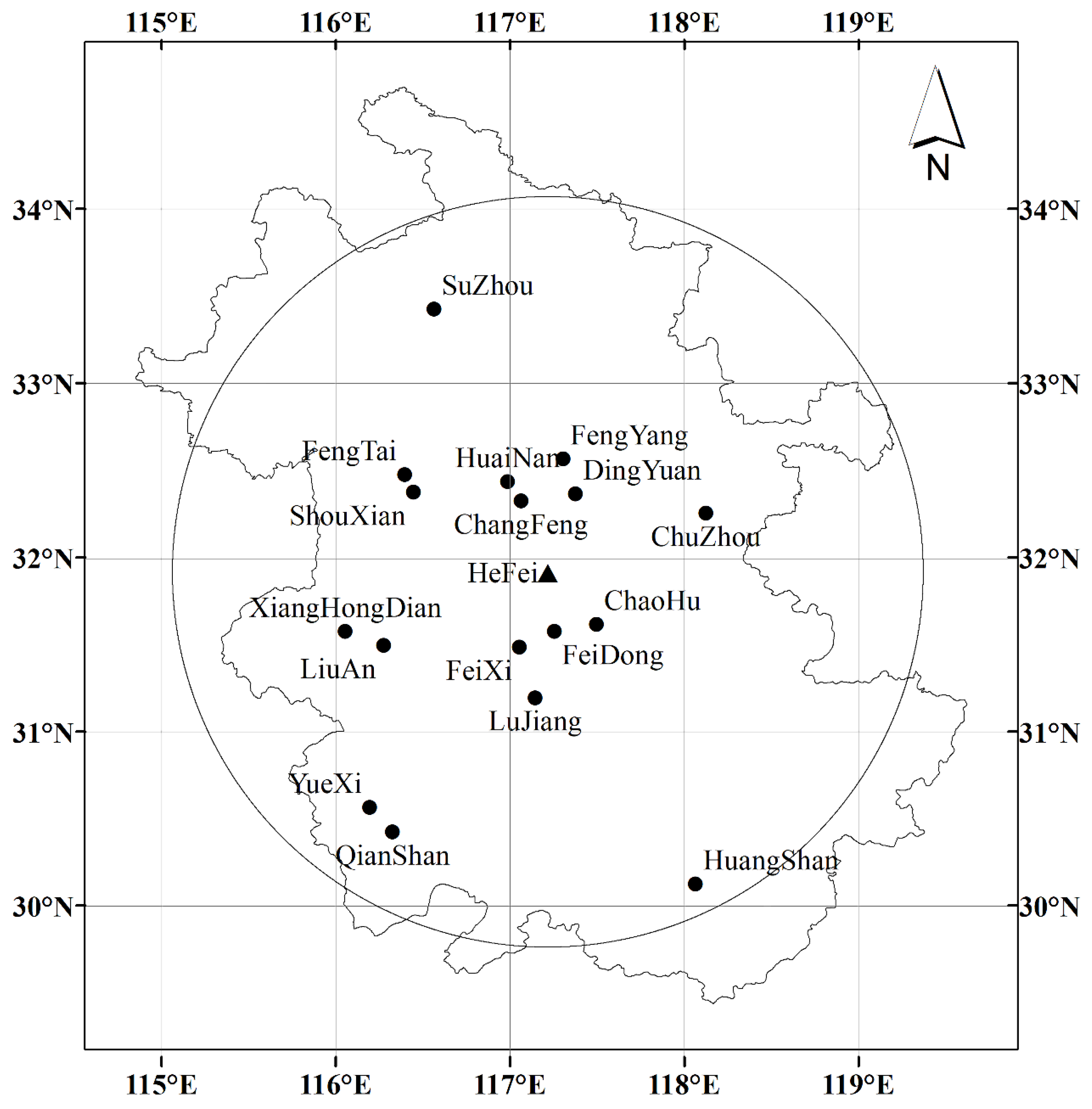
Figure 1.
The station distribution map, in which the dots are the disdrometers, the triangle in the center is the radar, and the circle is the 230 km detection range of the radar.
Figure 1.
The station distribution map, in which the dots are the disdrometers, the triangle in the center is the radar, and the circle is the 230 km detection range of the radar.
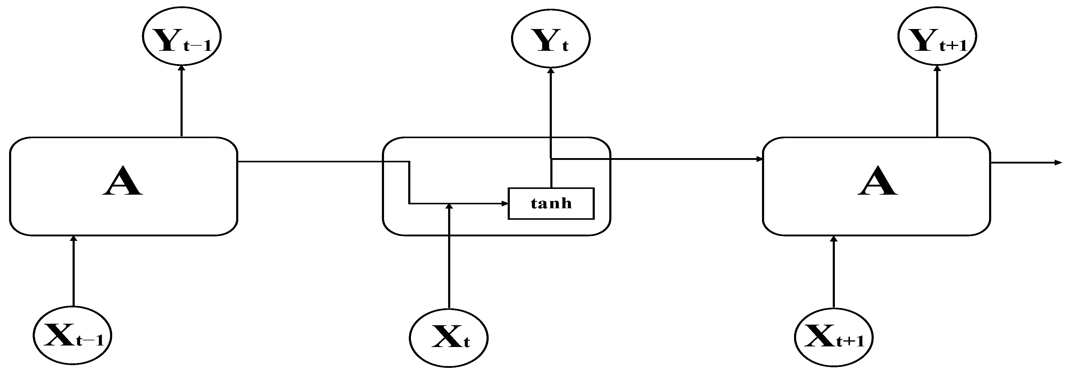
Figure 2.
The schematic diagram of RNN network.
Figure 2.
The schematic diagram of RNN network.
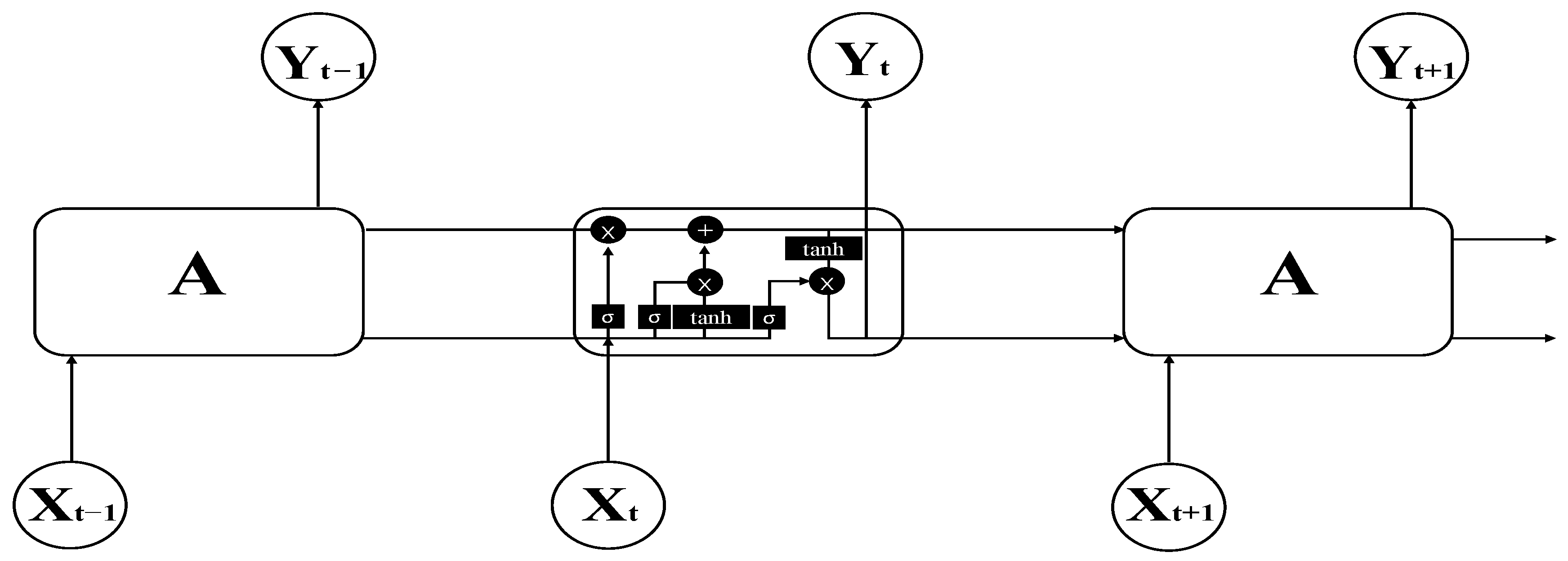
Figure 3.
The schematic diagram of LSTM network.
Figure 3.
The schematic diagram of LSTM network.
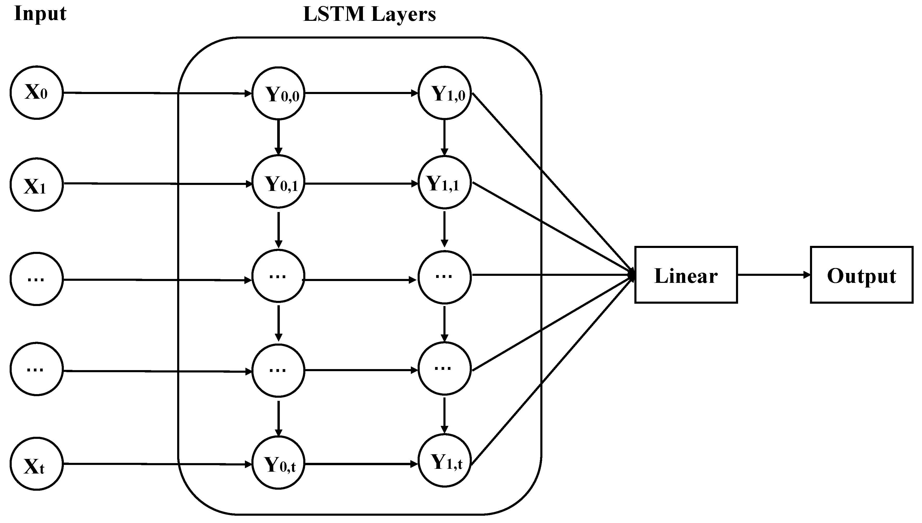
Figure 4.
The schematic diagram of DSDnet network.
Figure 4.
The schematic diagram of DSDnet network.
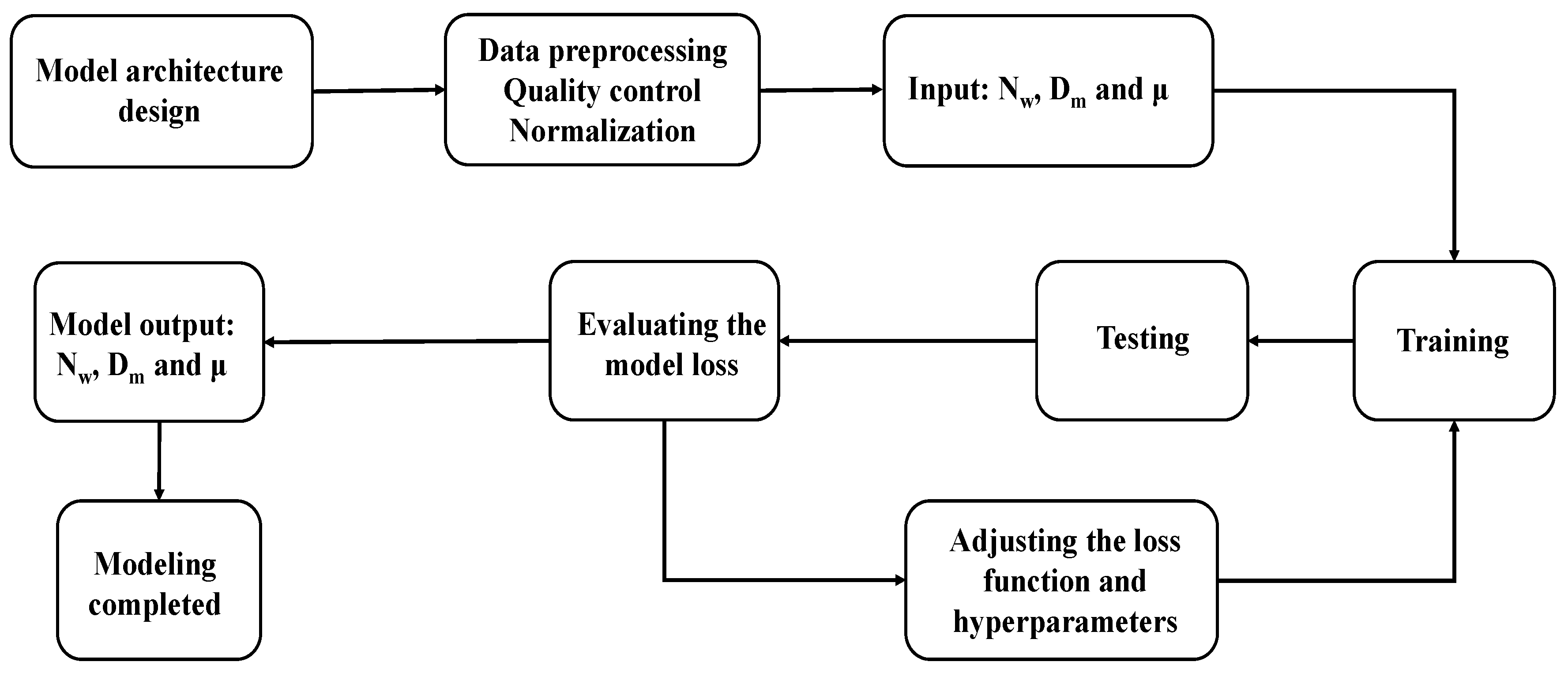
Figure 5.
The modeling flow chart.
Figure 5.
The modeling flow chart.
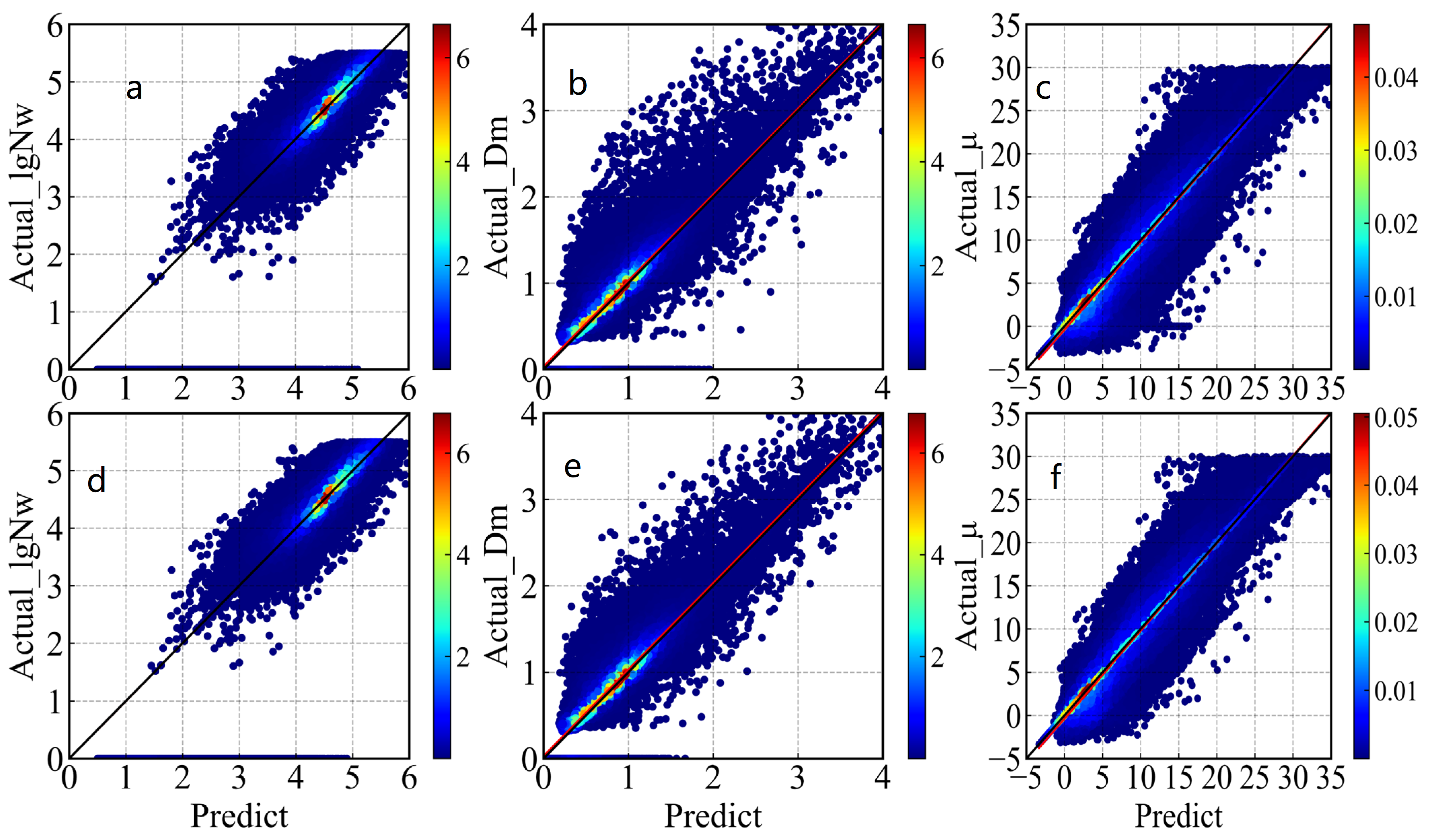
Figure 6.
The 12-min scatter plot of lgNw, Dm, and μ fitted by the observed data and predicted by the model, in which (a–c) are modeled with MLF and (d–f) with SLF. The red line denotes a linear trend line of the scattered points, and the color mark represents the Gaussian kernel density estimation.
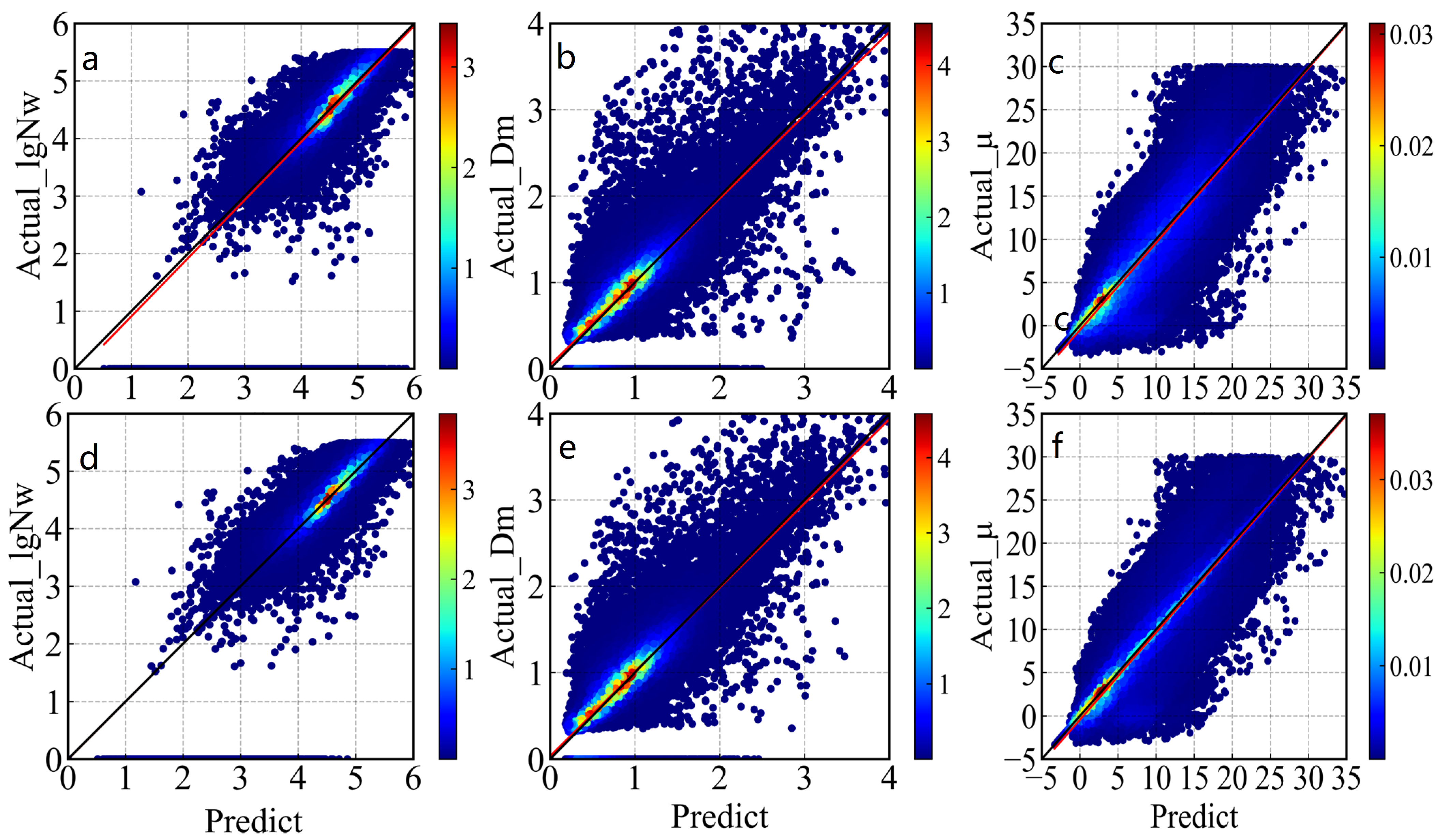
Figure 7.
The 30-min scatter plot of lgNw, Dm, and μ fitted by the observed data and predicted by the model, in which (a–c) are modeled with MLF and (d–f) with SLF. The red line denotes a linear trend line of the scattered points, and the color mark represents the Gaussian kernel density estimation.
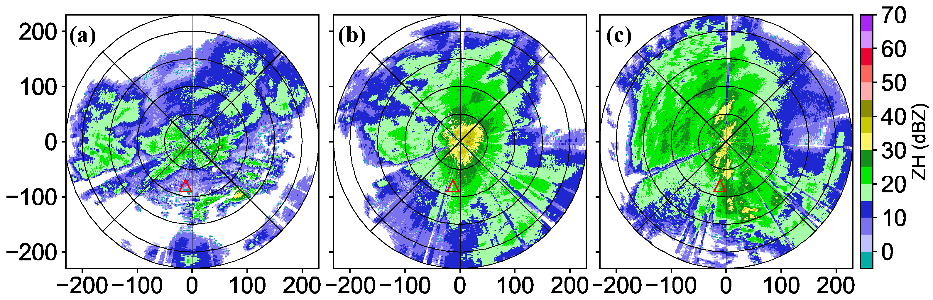
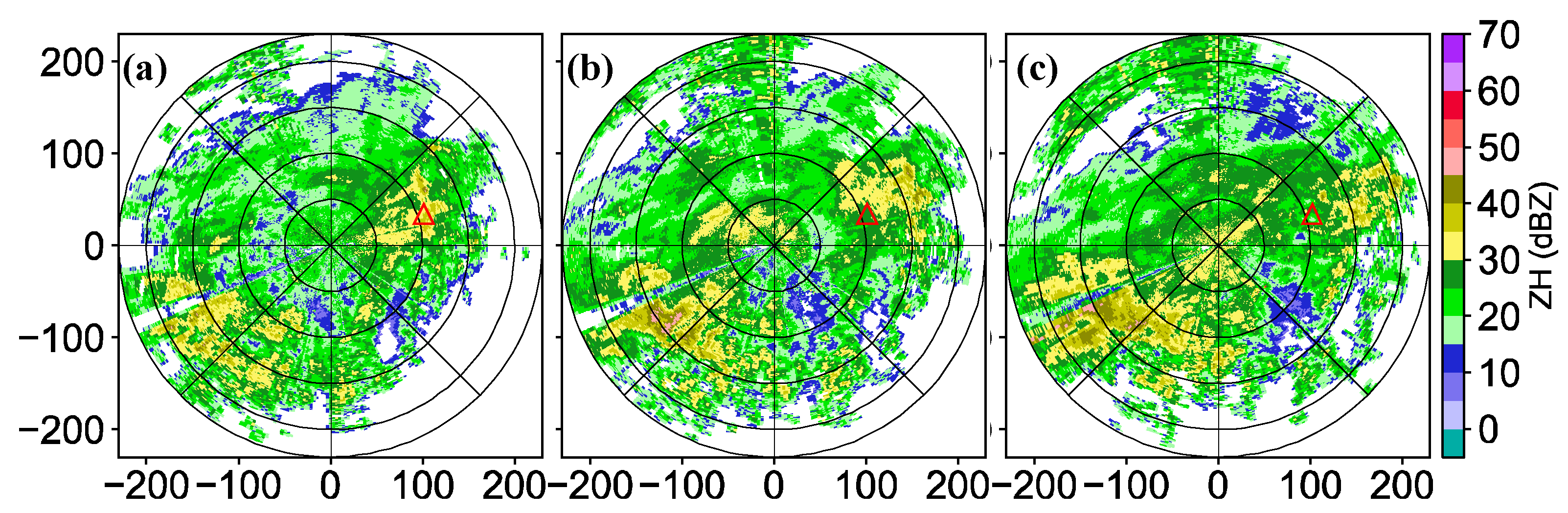
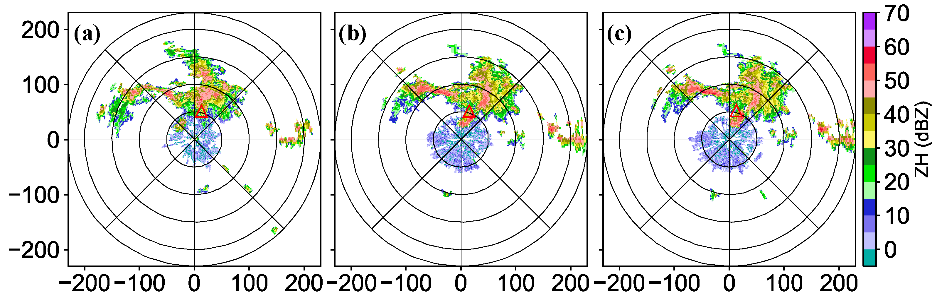
Figure 8.
The 0.5° PPI of reflectivity of the Hefei radar at 0726 (a), 0127 (b), and 1332 LST (c) on 26 January 2020, in which the red triangle is the location of the disdrometer at Lujiang, and the scale on the coordinate axes represents the distance (km).
Figure 8.
The 0.5° PPI of reflectivity of the Hefei radar at 0726 (a), 0127 (b), and 1332 LST (c) on 26 January 2020, in which the red triangle is the location of the disdrometer at Lujiang, and the scale on the coordinate axes represents the distance (km).
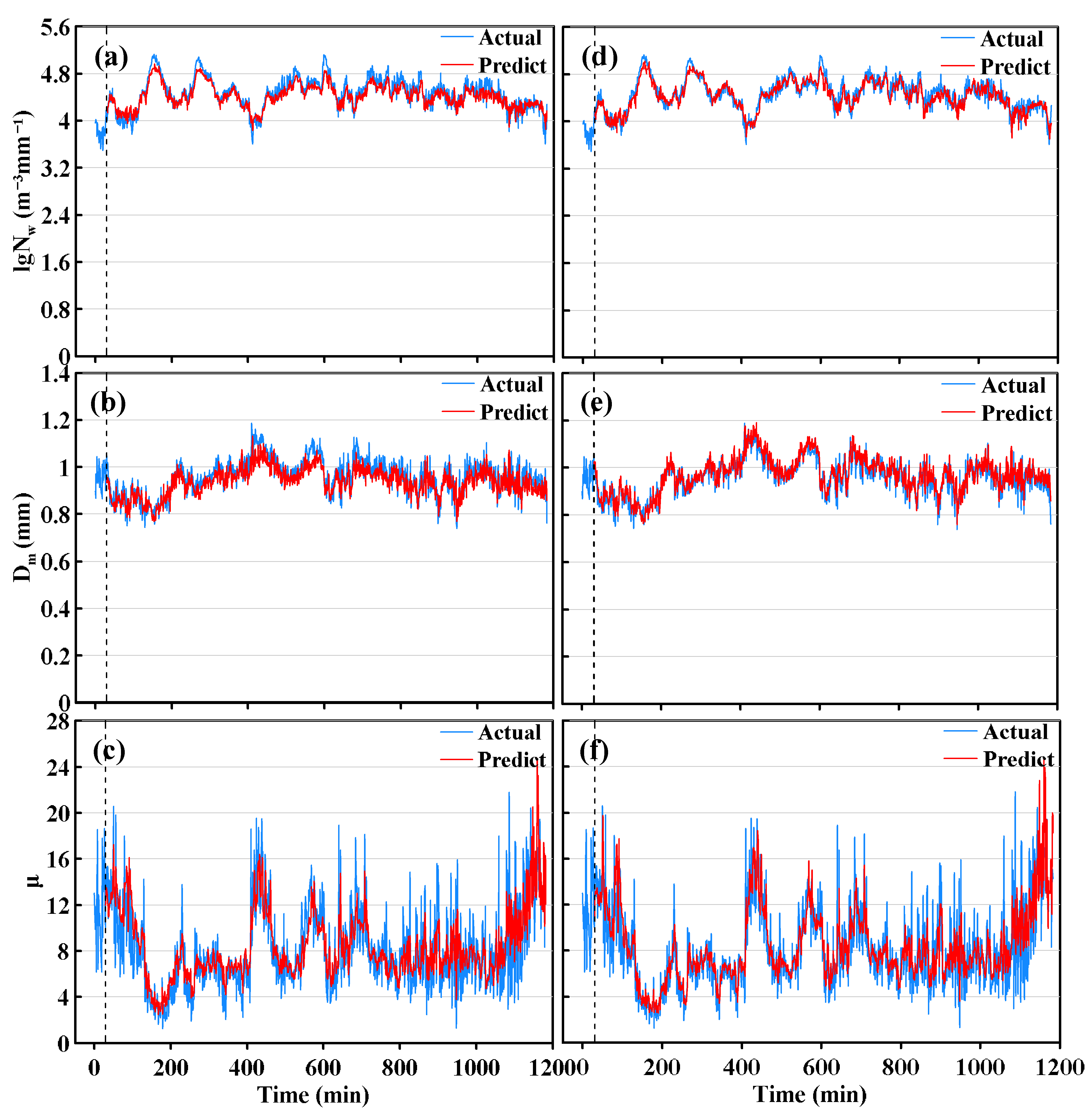
Figure 9.
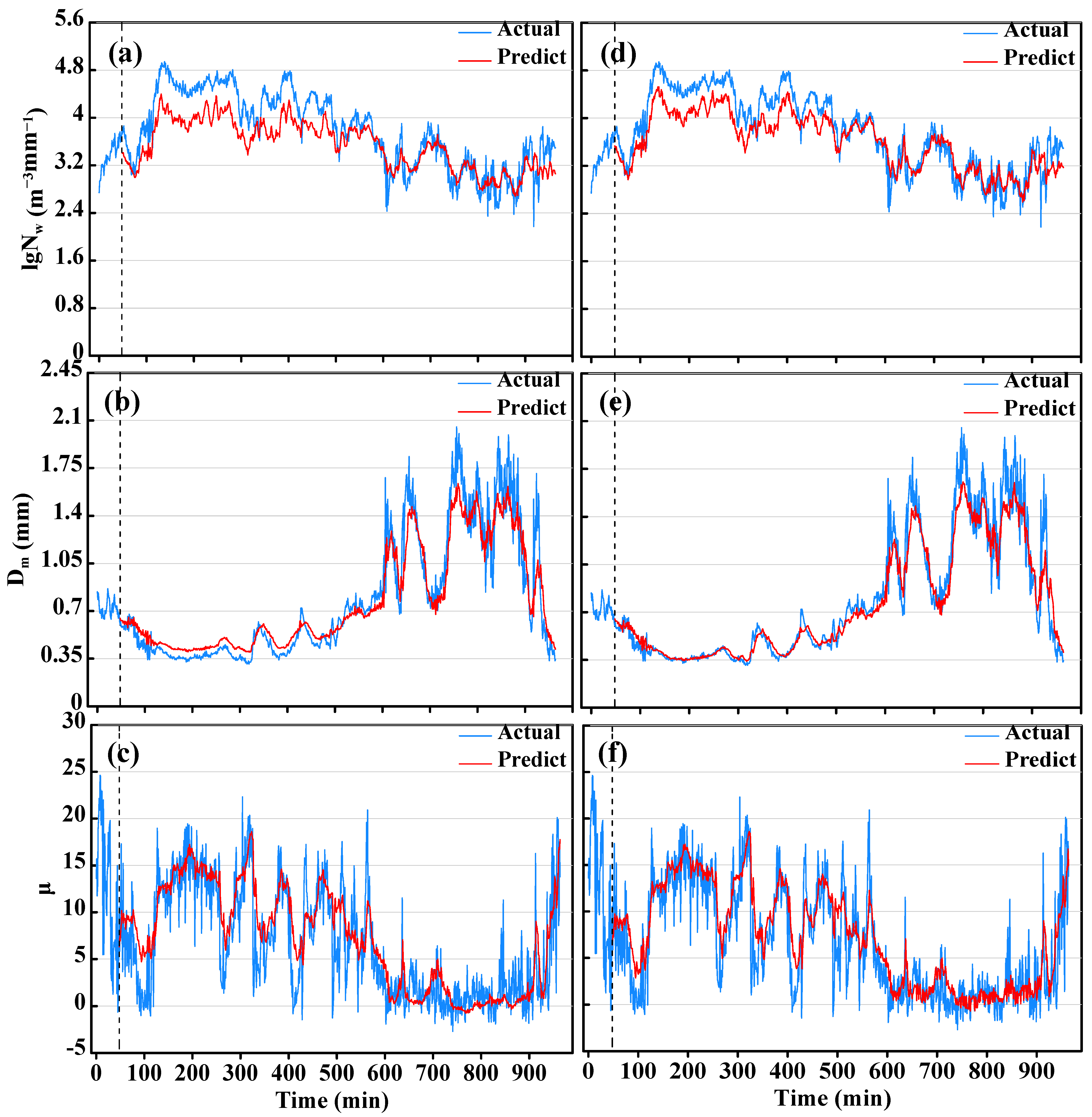
The curve of the 12-min prediction for the stratiform cloud precipitation case, in which the horizontal axes are rainfall duration time (min); vertical axes are (a,d) lgNw, (b,e) Dm (mm), and (c,f) μ; the red and blue curves represent the predicted and actual values; and the vertical dotted line is at the minute of Tstep + Mpred. Modeling with MLF is shown on the left (a–c), and with SLF on the right (d–f).
Figure 9.
The curve of the 12-min prediction for the stratiform cloud precipitation case, in which the horizontal axes are rainfall duration time (min); vertical axes are (a,d) lgNw, (b,e) Dm (mm), and (c,f) μ; the red and blue curves represent the predicted and actual values; and the vertical dotted line is at the minute of Tstep + Mpred. Modeling with MLF is shown on the left (a–c), and with SLF on the right (d–f).
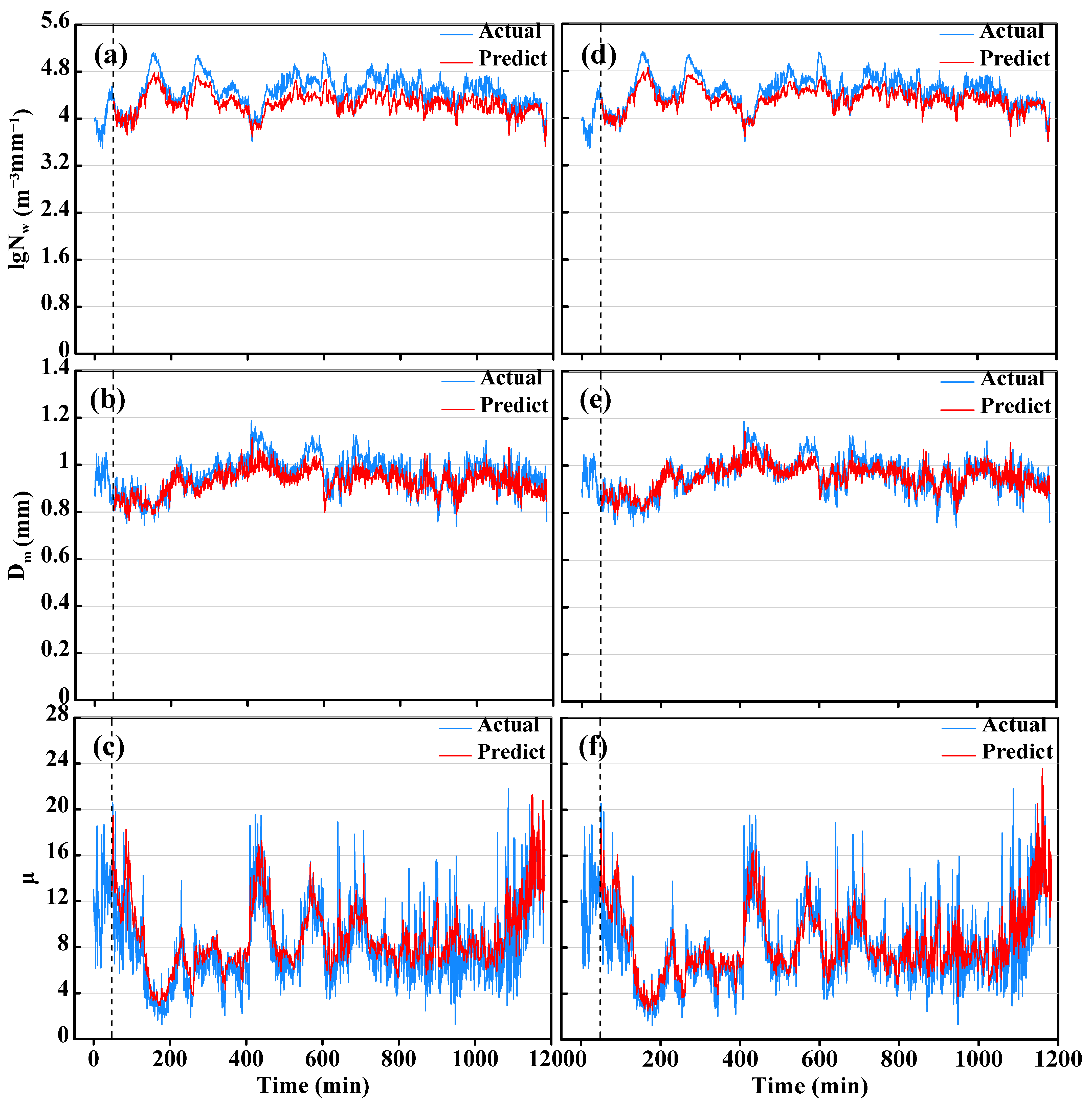
Figure 10.
The curve of the 30-min prediction for the stratiform cloud precipitation case, in which the horizontal axes are rainfall duration time (min); vertical axes are (a,d) lgNw, (b,e) Dm (mm), and (c,f) μ; the red and blue curves represent the predicted and actual values; and the vertical dotted line is at the minute of Tstep + Mpred. Modeling with MLF is shown on the left (a–c), and with SLF on the right (d–f).
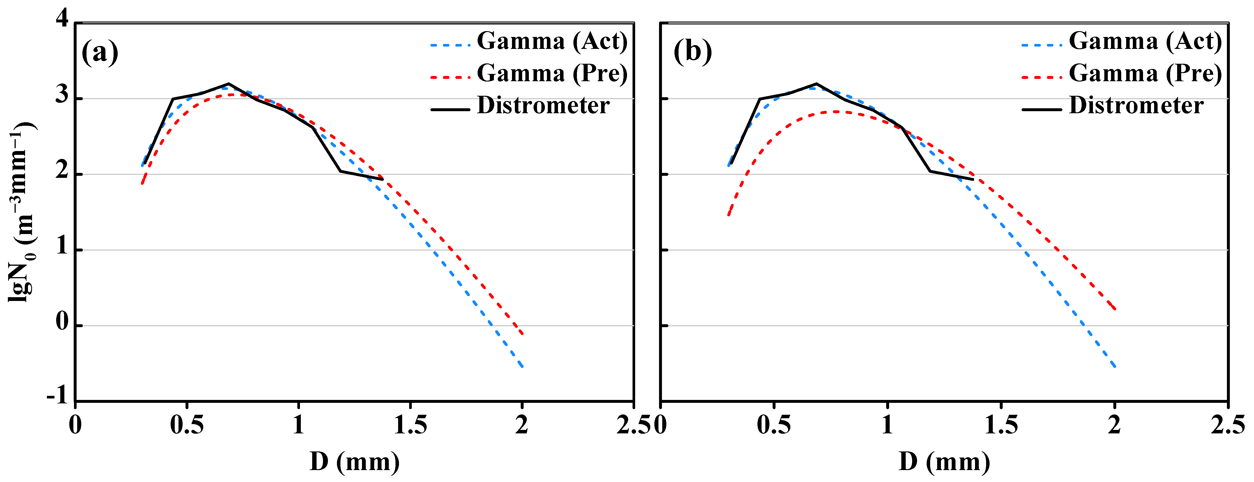
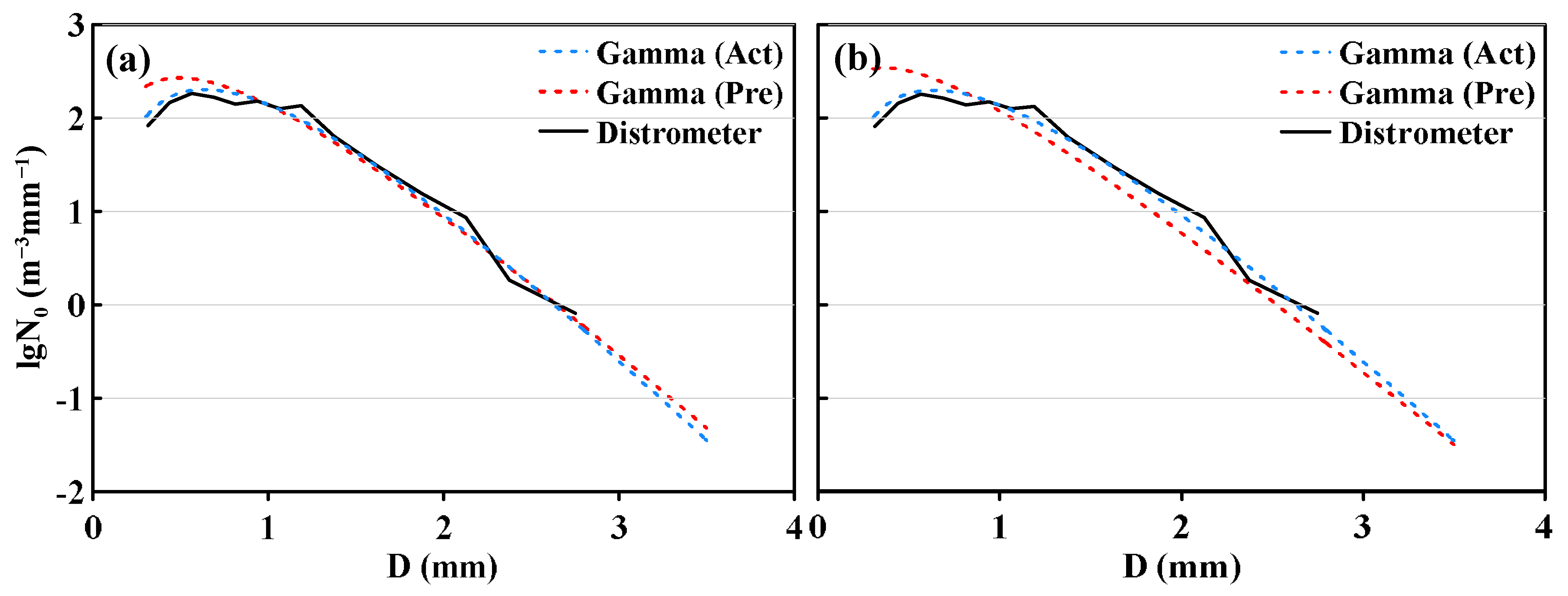
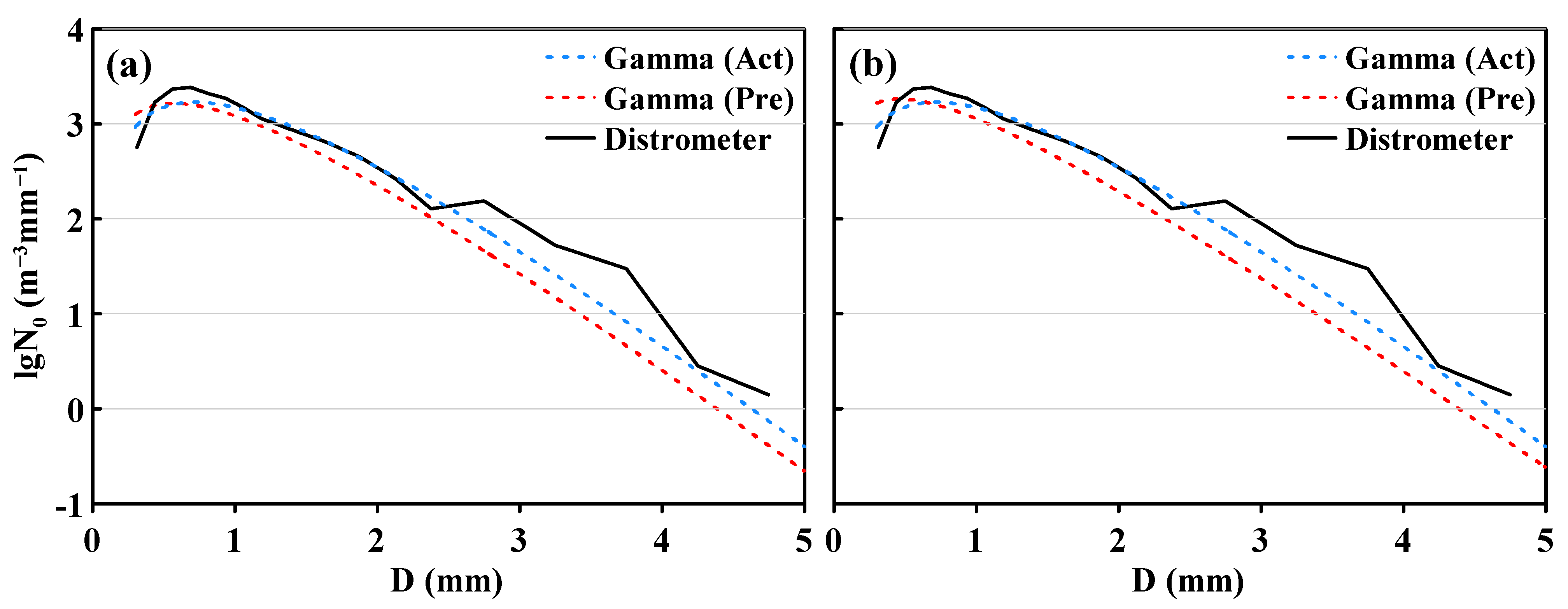
Figure 11.
The DSDs of measurement (black solid line), Gamma fitting (blue dotted line), and model prediction (red dotted line, (a) 12-min and (b) 30-min prediction) at the 1063rd min of this stratiform cloud precipitation case.
Figure 11.
The DSDs of measurement (black solid line), Gamma fitting (blue dotted line), and model prediction (red dotted line, (a) 12-min and (b) 30-min prediction) at the 1063rd min of this stratiform cloud precipitation case.
Figure 12.
The 0.5° PPI of reflectivity of the Hefei radar at 0818 (a), 0914 (b), and 0949 LST (c) on 24 November 2015, in which the red triangle is the location of the disdrometer at ChuZhou.
Figure 12.
The 0.5° PPI of reflectivity of the Hefei radar at 0818 (a), 0914 (b), and 0949 LST (c) on 24 November 2015, in which the red triangle is the location of the disdrometer at ChuZhou.
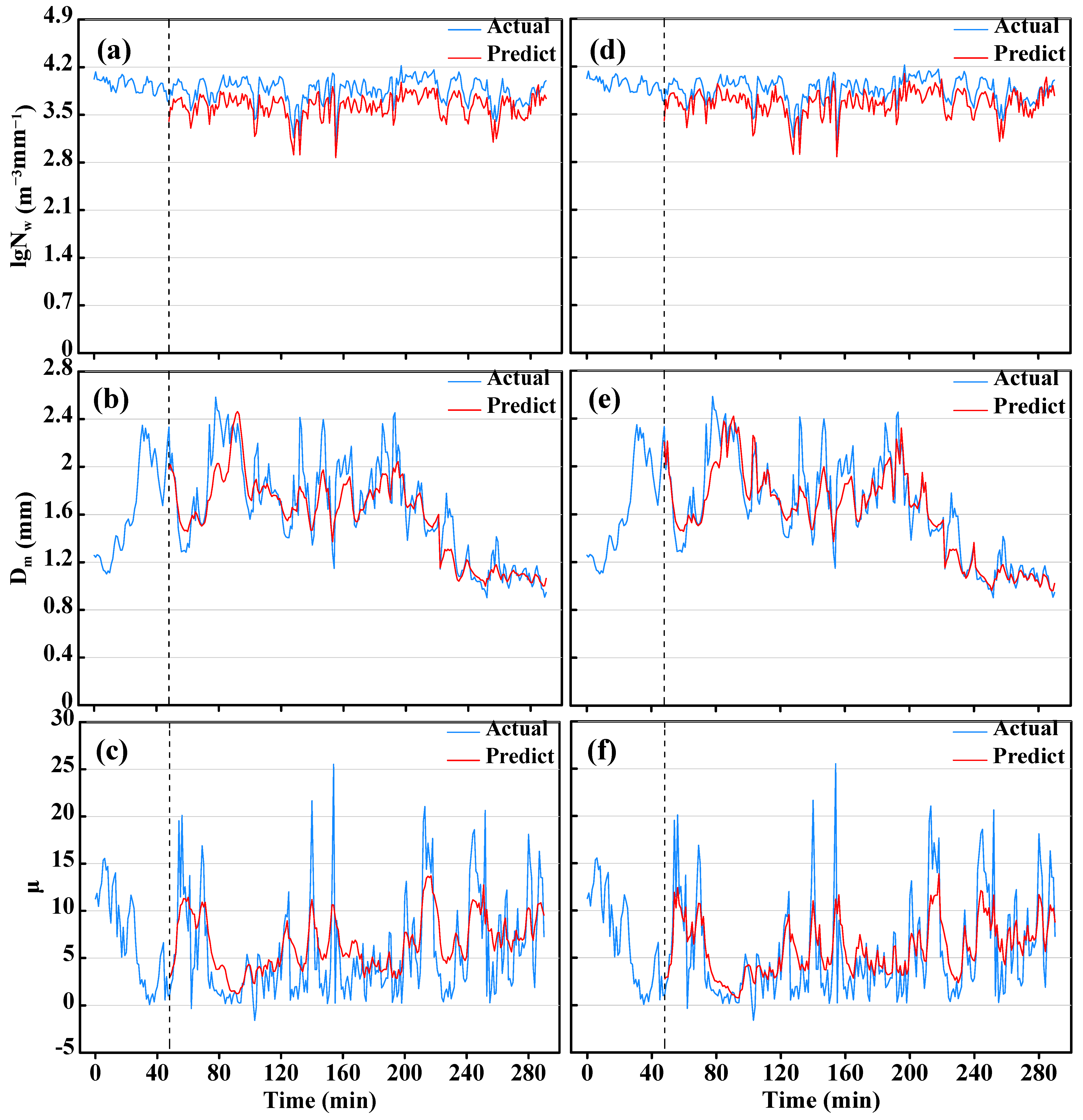
Figure 13.
The curve of the 30-min prediction for the mixed convective–stratiform cloud precipitation case, in which the horizontal axes are rainfall duration time (min); vertical axes are (a,d) lgNw, (b,e) Dm (mm), and (c,f) μ; the red and blue curves represent the predicted and actual values; and the vertical dotted line is at the minute of Tstep + Mpred. Modeling with MLF is shown on the left (a–c), and with SLF on the right (d–f).
Figure 14.
The DSDs of measurement (black solid line), Gamma fitting (blue dotted line), and model prediction (red dotted line, (a) 12-min and (b) 30-min prediction) at the 594th min of this mixed convective-stratiform cloud precipitation case.
Figure 14.
The DSDs of measurement (black solid line), Gamma fitting (blue dotted line), and model prediction (red dotted line, (a) 12-min and (b) 30-min prediction) at the 594th min of this mixed convective-stratiform cloud precipitation case.
Figure 15.
The 0.5° PPI of reflectivity of the Hefei radar at 0436 (a), 0522 (b), and 0528 LST (c) on 29 June 2015, in which the red triangle is the location of the disdrometer at Dingyuan.
Figure 15.
The 0.5° PPI of reflectivity of the Hefei radar at 0436 (a), 0522 (b), and 0528 LST (c) on 29 June 2015, in which the red triangle is the location of the disdrometer at Dingyuan.
Figure 16.
The curve of the 30-min prediction for the convective cloud precipitation case, in which the horizontal axes are rainfall duration time (min); vertical axes are (a,d) lgNw, (b,e) Dm (mm), and (c,f) μ; the red and blue curves represent the predicted and actual values; and the vertical dotted line is at the minute of Tstep + Mpred. Modeling with MLF is shown on the left (a–c), and with SLF on the right (d–f). Results of 30-min Prediction.
Figure 17.
The DSDs of measurement (black solid line), Gamma fitting (blue dotted line), and model prediction (red dotted line, (a) 12-min and (b) 30-min prediction) at the 86th min of this convective cloud precipitation case.
Figure 17.
The DSDs of measurement (black solid line), Gamma fitting (blue dotted line), and model prediction (red dotted line, (a) 12-min and (b) 30-min prediction) at the 86th min of this convective cloud precipitation case.
Table 1.
The performance parameters of the raindrop disdrometer.
Table 1.
The performance parameters of the raindrop disdrometer.
| Items | Parameters |
|---|
| Average falling speed of channel 1–32 (m/s) | Range | 0.2~20 |
| Classification | 0.05, 0.15, 0.25, 0.35, 0.45, 0.55, 0.65, 0.75, |
| 0.85, 0.95, 1.10, 1.30, 1.50, 1.70, 1.90, 2.20, |
| 2.60, 3.00, 3.40, 3.80, 4.40, 5.20, 6.00, 6.80, |
| 7.60, 8.80, 10.40, 12.00, 13.60, 15.20, 17.60, |
| 20.80 |
| Average particle diameter of 1–32 channels (mm) | Range | 0.2~25 |
| Classification | 0.062, 0.187, 0.312, 0.437, 0.562, 0.687, 0.812, |
| 0.937, 1.062, 1.187, 1.375, 1.625, 1.875, 2.125, |
| 2.375, 2.750, 3.250, 3.750, 4.250, 4.750, 5.500, |
| 6.500, 7.500, 8.500, 9.500, 11.000, 13.000, |
| 15.000, 17.000, 19.000, 21.500, 24.500 |
| Accuracy | liquid | ±5% |
| solid | ±20% |
| Particle level | | 32 (size) × 32 (velocity) |
| Differentiation of precipitation types | | >97% |
| Measurement interval | | 60 s |
| Measuring area | | 54 cm2 (18 cm × 3 cm) |
| Wavelength | | 780 nm (OTT Parsivel2) |
| | 650 nm (HSC-OTT Parsivel EF) |
| Output rating | | 0.5 mW (OTT Parsivel2) |
| | 3 mW (HSC-OTT Parsivel EF) |
Table 2.
The weight coefficient vectors of SLF in different value regions.
Table 2.
The weight coefficient vectors of SLF in different value regions.
| Parameter | W | L |
|---|
| Nw | 10, 5, 2, 5, 8, 10 | 0.54, 0.63, 0.72, 0.81, 0.90, 1 |
| Dm | 10, 5, 2, 5, 8, 10 | 0.14, 0.29, 0.44, 0.74, 0.89, 1 |
| μ | 10, 5, 2, 5, 8, 10 | 0.06, 0.16, 0.25, 0.44, 0.64, 1 |
Table 3.
The 12-min prediction evaluation results of the test set.
Table 3.
The 12-min prediction evaluation results of the test set.
| Model | Evaluation Index | lgNw | Dm | μ |
|---|
| | MRE | 0.05452 | 0.11925 | 0.16559 |
| With MLF | MAE | 0.23862 | 0.13497 | 1.43105 |
| | CC | 0.93162 | 0.89621 | 0.87996 |
| | MRE | 0.05235 | 0.11561 | 0.15486 |
| With SLF | MAE | 0.23251 | 0.13084 | 1.34834 |
| | CC | 0.93403 | 0.90934 | 0.89741 |
Table 4.
The 30-min prediction evaluation results of test set.
Table 4.
The 30-min prediction evaluation results of test set.
| Model | Evaluation Index | lgNw | Dm | μ |
|---|
| | MRE | 0.06867 | 0.17442 | 0.27311 |
| With MLF | MAE | 0.29384 | 0.15411 | 2.36024 |
| | CC | 0.85564 | 0.83968 | 0.82761 |
| | MRE | 0.05983 | 0.16188 | 0.24224 |
| With SLF | MAE | 0.25354 | 0.14287 | 2.01193 |
| | CC | 0.87599 | 0.85261 | 0.84564 |
Table 5.
The 12-min prediction evaluation results of stratiform clouds.
Table 5.
The 12-min prediction evaluation results of stratiform clouds.
| Model | Evaluation Index | lgNw | Dm | μ |
|---|
| | MRE | 0.02231 | 0.03545 | 0.17484 |
| With MLF | MAE | 0.09959 | 0.03395 | 1.41840 |
| | CC | 0.88919 | 0.86223 | 0.84995 |
| | MRE | 0.02181 | 0.02697 | 0.15086 |
| With SLF | MAE | 0.09739 | 0.02583 | 1.22393 |
| | CC | 0.90978 | 0.91626 | 0.86207 |
Table 6.
The 30-min prediction evaluation results for stratiform clouds.
Table 6.
The 30-min prediction evaluation results for stratiform clouds.
| Model | Evaluation Index | lgNw | Dm | μ |
|---|
| | MRE | 0.04846 | 0.04277 | 0.22196 |
| With MLF | MAE | 0.21637 | 0.04096 | 1.80071 |
| | CC | 0.84809 | 0.82457 | 0.79582 |
| | MRE | 0.03989 | 0.03633 | 0.17516 |
| With SLF | MAE | 0.18024 | 0.03288 | 1.43994 |
| | CC | 0.87736 | 0.83032 | 0.84207 |
Table 7.
The 30-min prediction evaluation results of mixed convective-stratiform clouds.
Table 7.
The 30-min prediction evaluation results of mixed convective-stratiform clouds.
| Model | Evaluation Index | lgNw | Dm | μ |
|---|
| | MRE | 0.14235 | 0.08697 | 0.41552 |
| With MLF | MAE | 0.11261 | 0.33545 | 2.63504 |
| | CC | 0.90904 | 0.89730 | 0.81276 |
| | MRE | 0.12532 | 0.06654 | 0.33504 |
| With SLF | MAE | 0.09185 | 0.28565 | 2.43201 |
| | CC | 0.92786 | 0.91974 | 0.84736 |
Table 8.
The 30-min prediction evaluation results of convective clouds.
Table 8.
The 30-min prediction evaluation results of convective clouds.
| Model | Evaluation Index | lgNw | Dm | μ |
|---|
| | MRE | 0.08276 | 0.09283 | 0.47653 |
| With MLF | MAE | 0.32051 | 0.15222 | 2.85232 |
| | CC | 0.74374 | 0.86702 | 0.71285 |
| | MRE | 0.06727 | 0.07619 | 0.37871 |
| With SLF | MAE | 0.28180 | 0.13494 | 2.46677 |
| | CC | 0.79573 | 0.88387 | 0.76503 |


 ,
, 


