Technical Note

Use of Remote Sensing Techniques to Estimate Plant Diversity within Ecological Networks: A Worked Example

by
Francesco Liccari
1,2,*,
Maurizia Sigura
2 and
Giovanni Bacaro
1
1
Department of Life Sciences, University of Trieste, Via L. Giorgieri 10, 34127 Trieste, Italy
2
Department of Agricultural, Food, Environmental and Animal Sciences, University of Udine, Via delle Scienze 206, 33100 Udine, Italy
*
Author to whom correspondence should be addressed.
Remote Sens. 2022, 14(19), 4933; https://doi.org/10.3390/rs14194933
Submission received: 29 June 2022 / Revised: 27 September 2022 / Accepted: 28 September 2022 / Published: 2 October 2022
(This article belongs to the Special Issue Remote Sensing of Ecosystem Diversity)

Abstract

:
As there is an urgent need to protect rapidly declining global diversity, it is important to identify methods to quickly estimate the diversity and heterogeneity of a region and effectively implement monitoring and conservation plans. The combination of remotely sensed and field-collected data, under the paradigm of the Spectral Variation Hypothesis (SVH), represents one of the most promising approaches to boost large-scale and reliable biodiversity monitoring practices. Here, the potential of SVH to capture information on plant diversity at a fine scale in an ecological network (EN) embedded in a complex landscape has been tested using two new and promising methodological approaches: the first estimates α and β spectral diversity and the latter ecosystem spectral heterogeneity expressed as Rao’s Quadratic heterogeneity measure (Rao’s Q). Both approaches are available thanks to two brand-new R packages: “biodivMapR” and “rasterdiv”. Our aims were to investigate if spectral diversity and heterogeneity provide reliable information to assess and monitor over time floristic diversity maintained in an EN selected as an example and located in northeast Italy. We analyzed and compared spectral and taxonomic α and β diversities and spectral and landscape heterogeneity, based on field-based plant data collection and remotely sensed data from Sentinel-2A, using different statistical approaches. We observed a positive relationship between taxonomic and spectral diversity and also between spectral heterogeneity, landscape heterogeneity, and the amount of alien species in relation to the native ones, reaching a value of R2 = 0.36 and R2 = 0.43, respectively. Our results confirmed the effectiveness of estimating and mapping α and β spectral diversity and ecosystem spectral heterogeneity using remotely sensed images. Moreover, we highlighted that spectral diversity values become more effective to identify biodiversity-rich areas, representing the most important diversity hotspots to be preserved. Finally, the spectral heterogeneity index in anthropogenic landscapes could be a powerful method to identify those areas most at risk of biological invasion.

1. Introduction

As there is an urgent need to protect rapidly declining global diversity [1], it is important to identify methods to quickly estimate the diversity and heterogeneity of a region and effectively implement monitoring and conservation plans. It is well known that biodiversity assessment through field surveys has a very high cost both in terms of time and money. Economic limitations often cause the inability to implement monitoring programs based on large-scale fieldwork [2]. Biodiversity monitoring programs must be planned on a sound basis to obtain quality information and three aspects are considered particularly relevant, i.e., sampling design, sample size, and type of statistical analysis [3,4]. These requirements make it complex to obtain statistically valid monitoring data for better understanding and modeling of biodiversity over space and time [5]. In contrast to traditional field-based samplings, Earth Observation and Remote sensing (RS/EO), based on airborne and satellite systems, provides data and methods that, complementing field-based techniques, are particularly useful for biodiversity monitoring, as it allows the observation of regions with a high spatial and temporal resolution, thus enabling the production of maps for modeling and monitoring diversity from local to global scales [6,7,8]. Operational methods for detecting biodiversity patterns and ecosystem heterogeneity using remote-sensing data require minimal supervision and do not rely on extensive ground-based data collection, as they are non-expensive and ready-to-use methods [9]. From this point of view, the development of free and open-source algorithms to measure and monitor biodiversity and/or ecosystem heterogeneity from space provide robust, reproducible, and standardized estimates of ecosystem functioning and services [10].
The combination of remotely sensed and field-collected data represents one of the most promising approaches to boost large scale and reliable biodiversity monitoring practices [2]. To date, much research has considered the relationships between remotely sensed and field-sampled data (e.g., [11,12,13]) under the paradigm of the Spectral Variation Hypothesis (SVH), proposed for the first time by Palmer et al. [11] and further developed by Rocchini et al. [14,15]. This concept hypothesizes that the variability of the spectral response of a remotely sensed image could be used as a proxy to assess plant biodiversity. The ability of SVH to detect plant diversity was tested on several ecosystems covering large areas (e.g., [16,17,18]), but few studies (e.g., [19]) have investigated SVH application at a greater level of detail over small, complex, and heterogeneous areas.
Typically, in these studies, diversity is assessed in term of α and β components [20,21], accounting for taxonomic diversity in ground-based data as well as for spectral diversity in remotely sensed data. Specifically, α diversity represents local diversity or diversity within a community and β diversity represents compositional variation among communities. Furthermore, another often neglected component of ecological diversity is represented by ecosystem heterogeneity that is linked to a range of ecological processes and functions that, in addition to species diversity patterns and change [8], includes metapopulation dynamics [22], population connectivity [23] or gene flow [24].
Here, we decided to test the potential of SVH to capture information on plant diversity at fine scale in a complex landscape, computing both α and β components and ecosystem heterogeneity via remote sensing. The two new and promising methodological approaches for estimating α and β spectral diversity and ecosystem heterogeneity have been tested using the R packages “biodivMapR” [9,16] and “rasterdiv” [25,26], respectively. Specifically, we investigated whether spectral diversity and heterogeneity can be used as proxies for taxonomic diversity and landscape heterogeneity. In more detail, (i) we examined whether the α and β components of spectral diversity can be compared with α and β taxonomic diversity and (ii) whether spectral heterogeneity (measured as pixel reflectance variation) is related to landscape heterogeneity and plant diversity in a complex landscape, where natural and anthropogenic elements interact. The objective was to understand if spectral data can be used to assess and/or monitor plant diversity and its dynamics in an Ecological Network (EN) or more generally in natural environments over time.
We tested the reliability of the two methodological approaches on an existing EN located in Friuli Venezia Giulia region (northeastern Italy), which was developed at the local scale in the context of the Regional Environmental Landscape Plan [27]. The considered EN was modeled as a composite multi-species ecological network where the nodes (natural habitats), corridors (links between natural habitats) capture favorable conditions for biodiversity in an agricultural landscape matrix. Most of these natural habitats are wetlands which are vulnerable ecosystems under climate change, extremely important for the maintenance of biodiversity and among the most exploited and impacted by human activity especially in Europe [28,29,30]. These environments are usually characterized by marked vegetation zonation, associated with the environmental gradients, determined primarily by hydrology [31], which host numerous species, including rare and endemic ones.

2. Materials and Methods
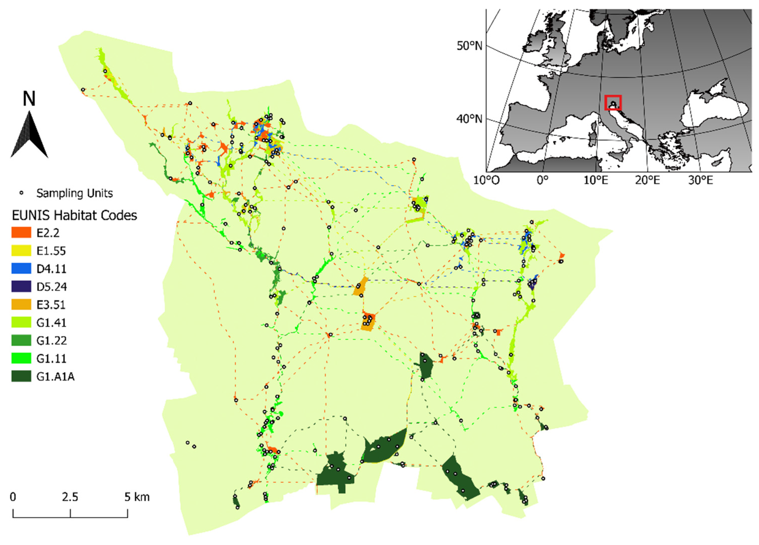
2.1. Study Site

This study was carried out in the lowlands of the Friuli Venezia Giulia region (NE Italy; centroid coordinates: 45°48′13.4″N–13°08′11.0″E; Figure 1). The study area has an extent of 298 km2 including a vast agricultural area bordered by two river systems (Stella and Corno). The landscape is characterized by a mixed mosaic of intensively and extensively cultivated areas, settlements, semi-natural, and natural habitats, including eight Natura 2000 Special Area of Conservation (Habitats Directive 92/43/EEC) and nine regional protected sites (biotopes), mainly connecting wetland habitats.
The geology of the area consists mainly of Quaternary sand, silt, and silt-clay sediments formed by glacial fluvial transport during the Pleistocene and by alluvial deposition during the Holocene. The area is characterized by an average annual temperature of about 13 °C and an average annual precipitation between 1100 and 1400 mm.
The natural habitats of the area are woods, meadows, and fens and have been classified following EUNIS habitat classification [32,33]. Specifically part of the forests are dominated by Carpinus betulus and Quercus robur (EUNIS habitat codes G1.A1A) while the wet forests by Alnus glutinosa, Fraxinus spp., and Salix spp. (EUNIS habitat codes F3.23, F9.2, G1.11, G1.22, G1.41), dry meadows are characterized by Arrhenatherum elatius, Brachypodium rupestre, Bromopsis erecta, Carex spp., Chrysopogon gryllus, Festuca rubra, Filipendula vulgaris, Lolium spp., Lotus spp., Trifolium spp. (EUNIS habitat codes E1.55, E2.2) while wet meadows by Carex spp., Molinia spp., and Filipendula ulmaria (EUNIS habitat codes E3.4, E3.51) and fens by Armeria helodes (endemic), Cladium mariscus, Equisetum palustre, Frangula alnus, Lysimachia vulgaris, Molinia caerulea, Potentilla erecta, Salix cinerea, Scirpoides holoschoenus, Schoenus nigricans, and Senecio fontanicola (endemic; EUNIS habitat codes D4.11, D5.24).

2.2. Data Collection and Analysis

2.2.1. Sampling Units

Data on plant richness and composition were collected during a field campaign to characterize plant diversity in the EN (see Liccari et al. [34,35]). All EN nodes with an area over 1 ha were sampled. The sampling design chosen was hierarchical, with each habitat type sampled within each node, proportional to habitat extent within the node (Table S1). Sampling density in relation to habitat extent was chosen as follows: a square plot of 100 m2 was randomly placed for a habitat area <5 ha, 2 plots for an area ≥5 and ≤10 ha, and finally 3 plots for an area >10 ha. A total of 219 plots were randomly selected within the EN, corresponding to an overall sampling density of 0.13 plot/ha. Presence and abundance (% visual cover estimate) of each vascular plant species rooted in each plot were recorded. Nomenclature and taxonomy of species followed Bartolucci et al. [36] for native species and Galasso et al. [37] for alien species. Data were collected in the spring and summer of 2019 (193 plots) and 2020 (26 plots).

2.2.2. Satellite Data

The SVH has been tested using Sentinel-2 Level 2A (bottom of atmosphere) multispectral images with tile 33TUL for the year 2019, downloaded from Copernicus Open Access Hub [38], selecting only images with cloud cover of 0. The reflectance signal of the vegetation was derived from the Sentinel-2A’s multispectral instrument (MSI) on board, that measures the solar electromagnetic spectrum from 457 nm to 2280 nm with 13 bands.
The images were further processed using SNAP-ESA Sentinel Application Platform [39] to select the bands of interest (bands: 2, 3, 4, 5, 6, 7, 8, 8A, 11, 12) resampling them all to 10 m × 10 m spatial pixel resolution using bilinear interpolation and finally to crop the images with the extent of the study area. The selected bands were blue (B02, 458–523 nm), green (B03, 543–578 nm), red (B04, 650–680 nm), three red edges (B05, 698–713 nm; B06, 733–748 nm; B07, 773–793 nm), near infrared (B08, 785–899), near infrared narrow (B08A, 855–875 nm), and two short wave infrareds (B11, 1565–1655 nm; B12, 2100–2280 nm).

2.2.3. Spectral Diversity Estimation

We used the R package “biodivMapR” [9,16] for estimating spectral α and β diversity. The estimation method is based on the SVH and takes advantage of high spatial resolution multispectral information to differentiate species or groups of species based on the optical traits corresponding to the reflectance of each pixel [9,40,41]. We considered taxonomic diversity in ground-based data and spectral diversity in remotely sensed data. In general, α diversity, here taxonomic or spectral, summarizes the number of different elements (species or reflectance spectrum values) within sampling units and can be expressed as richness (i.e., the number of species) and evenness (i.e., their relative abundance) [16,20,21]. To consider both richness and evenness and compare spectral and taxonomic diversity values, we computed species richness and Shannon diversity index (H’, [42]).
β diversity, whether taxonomic or spectral, represents the variation among sampling units in both composition and abundance values [16,20,21]. β diversity in remotely sensed and field data was analyzed using the Bray–Curtis (BC) dissimilarity index [43]. This dissimilarity index is defined as the sum over the whole species of the ratio between the difference of abundance values and the sum of abundance values for each species, and it represents the vegetation plots (or spectral value of the pixels) pairwise differences using quantitative species abundance data. The BC dissimilarity index ranges between 0, when two plots share the same elements, and 1, when the two sampling units are totally different.
The package supports only one multispectral raster image at a time in its functions. Thus, we chose to use a satellite image taken on 3 June 2019, as it was the period with the most active green biomass and the most ground surveys carried out. Additionally, we chose to use multiple images and then averaging them across the sampling period (May–September 2019) to compare the different performance. The resulting Sentinel 2 multi-spectral images were filtered to remove non-vegetated, shaded, and cloudy pixels. The applied thresholds were as follows: (1) Normalized Difference Vegetation Index (NDVI) higher than 0 to exclude non-vegetated pixels, (2) NIR > 1500 to remove shaded areas as these are characterized by low overall reflectance, and (3) blue < 500 to ignore cloudy pixels as residuals from atmospheric corrections may lead to increased reflectance in the blue domain [9].
After the filtering, a Principal Component Analysis (PCA) was performed on a random subset (21% ca) of the image to ensure computational efficiency. The result of this PCA was then applied to order the whole image. Subsequently, a second filtering based on PCs thresholding was applied automatically discarding the pixels showing values beyond the mean PC value ± 3 standard deviations for any of the first five components and the mask was updated accordingly. Finally, the PCA preprocessing including random pixel selection was applied a second time with the updated mask. Based on PCA results, relevant features for biodiversity mapping were selected considering the PCA outputs.
Spectral species mapping is based on k-means clustering of the components selected from the PCA. First, a subset of pixel was extracted from PCA, equivalent to the number of pixels randomly selected when computing PCA. This pool of pixels was then split into n partitions, and k-means clustering was performed on each partition, in order to define the adequate number of clusters. The clustering was then applied to the whole PCA image in order to assign a cluster to each pixel based on closest centroid, for each repetition. Therefore, the number of partition cluster maps result from this independent clustering. Each cluster map was then processed until the computation of α- and β-diversity metrics, and these diversity metrics were finally averaged. Spectral species mapping was performed setting number of clusters parameter to 50. This value was suggested by Féret and de Boissieu [9] for tropical forests, but it was also indicated that the number of clusters should be set according to the level of heterogeneity of the landscape under study, in our case quite high.
The α and β spectral diversity maps were produced through the computation of three indexes (i.e., species richness and H’ for α diversity and BC for β diversity), based on the distribution of clusters in the spectral species map for a window size set to 6 × 6 pixels over the whole image. Testing different window sizes on the study area, we observed that the smaller the window, the more accurate the estimate, but small windows may not contain a sufficient number of pixels. For this reason, we decided to use a window of 6 × 6 pixels as a compromise. Finally, spectral diversity index values were extracted for the sampled plots (plots containing fewer than three pixels were discarded) in order to compare field inventories with diversity indices estimated by the “biodivMapR” package. We compared these values by linear regression, correlation analysis, and using the R package “Metrics” [44] that computes evaluation metrics (i.e., RMSE and bias) that are commonly used in supervised machine learning to compare actual and predicted values.

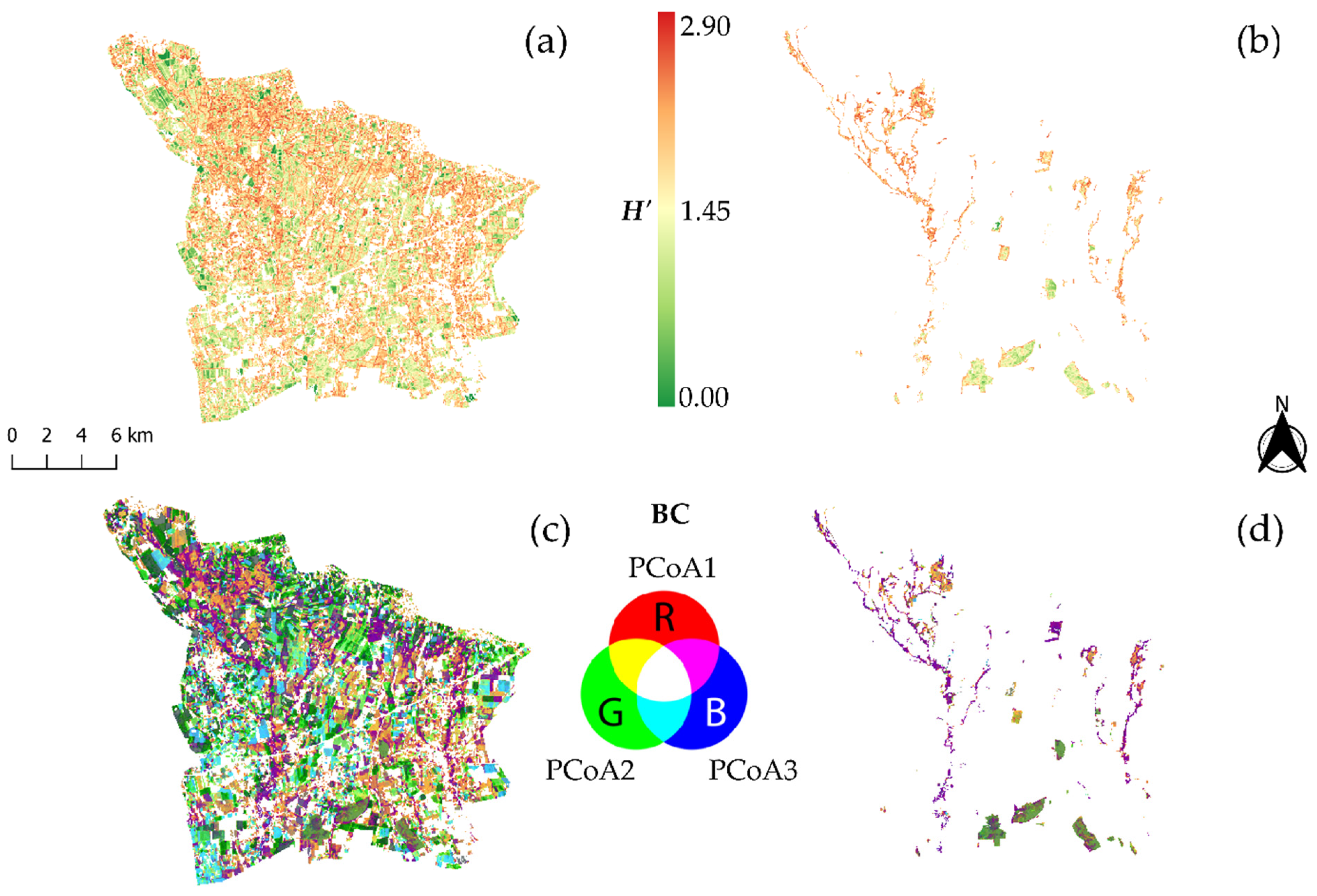
2.2.4. Spectral Ecosystem Heterogeneity Estimation

The “rasterdiv” package [25] provides a flow of functions based on information theory and generalized entropy, incorporating abundance information for each informative value but also on the relative numerical distance between these values [26]. We used this package for calculating the Rao’s Quadratic heterogeneity measure (hereafter Rao’s Q; [45]). It can be defined as the expected difference in reflectance values between two pixels drawn randomly with replacement from the evaluated set of pixels. The 10 selected bands from the Sentinel 2 image of 3 June 2019 were re-scaled to 8-bit radiometric resolution as suggested by Rocchini et al. [26] and a moving window of 9 × 9 pixels was used for calculating the index (Qmulti) and the weight for the distance matrix (alpha) was set to 1, 5, and infinite (see package vignette for more details, [25]). A larger window was used here since in this case, the larger the window the greater the accuracy of the heterogeneity index. Moreover, due to the transformation of the pixel value in 8-bit, a larger number of pixels was necessary to generate variability in the index calculation. In addition, we also calculated the Rao’s Q on an NDVI time series (i.e., one image per month for the year 2019; QNDVI) rescaled to 8-bit radiometric resolution, with a moving window of 9 × 9 pixels and alpha set to 1, 5, and infinite. Here again, Rao’s Q values were extracted for all the sampled plots and the relationships between spectral heterogeneity and field data were estimated using Generalized Additive Models (GAM) and transformation-based Redundancy Analysis (tb-RDA). We hypothesized that in a highly heterogeneous landscape, such as the one under study, relationships were to be sought between spectral heterogeneity, landscape heterogeneity, and the amount of native and alien species. For this reason, in the GAMs we considered Rao’s Q values deriving from both NDVI time series (QNDVI) and multispectral single image (Qmulti) as response variables and ratio of alien to native species richness (RatioAN) and Shannon index by land use category (ShannonLU) calculated in an area of 250 m around the plots as predictive variables.
Six GAMs were considered, the response variables were alternatively QNDVI1, QNDVI5, QNDVIInf, Qmulti1, Qmulti5, and QmultiInf, and the predictive variables were always ShannonLU as smooth term and RatioAN as linear term. A Gaussian distribution was used for the error and a cubic regression spline was selected for the smooth term by means of the “mgcv” R package [46]
Regarding β diversity, the contribution of previous variables (Qmulti, RatioAN, and ShannonLU) with the addition of three other variables (i.e., native species richness, N.Nat; focal species richness, N.Foc; and habitat type) to the observed community composition was considered using tb-RDA [47]. QNDVI and alien species richness were not considered as they were highly collinear with Qmulti and RatioAN, respectively. The tb-RDA was based on Hellinger [48] pre-transformed species composition matrix. Species abundances were log transformed before Hellinger transformation was done. These transformations were made possible as tb-RDA supports the use of many data transformations to perform ordination, offering much more flexibility for the analysis of community data [49]. Variance partitioning was then computed in order to assess which group of variables (habitat, land use, and Rao’s Q) contributed more to explain the variability in the community composition.

3. Results

3.1. Comparison of α and β Spectral Diversity vs. Measured Taxonomic Diversity

The resulting α and β spectral diversity maps, obtained from the “biodivMapR” package, are shown in Figure 2 and Figure S1.
The comparison between the observed values of α and β taxonomic diversity calculated from sampled plots and the ones remotely estimated via the “biodivMapR” are reported below.
Considering the results for the single image (3 June 2019, Figure S1), the regression between observed taxonomic and estimated spectral species richness (Figure S2a) gave an RMSE = 16.68 and a bias = 15.15 that indicate a high underestimation of the number of species. We also computed the Pearson correlation between the observed species richness and the estimated one obtaining a value of 0.16 (p = 0.03). This result was partly expected considering the study of Féret and Asner [16] where they observed an underestimation that could be explained by the limited number of spectral species compared to the maximum taxonomic diversity. However, as stated by Féret and Asner [16], it can be easily corrected with a linear factor derived from the relationship obtained between field data and estimation (for example, in our case by 0.4, Figure S2b).
The regression between observed taxonomic and estimated spectral H′ (Figure S3) yielded an RMSE = 0.39 in H’ units and a bias = −0.01 that indicated a slight overestimation of H’. We also computed the Pearson correlation between the observed H’ and the estimated H’ obtaining a value of 0.53 (p < 0.001). The regression between observed taxonomic and estimated spectral BC (Figure S4) yielded an RMSE = 0.17 in BC units and a bias = 0.06 that indicated a slight underestimation of BC dissimilarity. Mantel correlation between the observed BC and the estimated one yielded a value of 0.48 (p < 0.001).
Considering the results for the averaged multiple images (from May 2019 to September 2019, Figure 2), the regression between observed taxonomic and estimated spectral species richness gave an RMSE = 14.53 and a bias = 14.66 that indicate a high underestimation of the number of species. We also computed the Pearson correlation between the observed species richness and the estimated one obtaining a value of 0.18 (p = 0.01). In this case, the species richness estimation produced a slightly better result than that of the single image.
The regression between observed taxonomic and estimated spectral H′ (Figure S5) yielded an RMSE = 0.36 in H’ units and a bias = 0.06 that indicated a slight underestimation of H’. We also computed the Pearson correlation between the observed H’ and the estimated H’ obtaining a value of 0.60 (p < 0.001). The regression between observed taxonomic and estimated spectral BC (Figure S6) yielded an RMSE = 0.15 in BC units and a bias = 0.05 that indicated a slight underestimation of BC dissimilarity. Mantel correlation between the observed BC and the estimated one yielded a value of 0.52 (p < 0.001).
The spectral β diversity map, expressed as BC dissimilarity index, produced by the projection of the n × n dimensional space of the dissimilarity matrix into an n × 3 dimensional space (PCoAs, Figure 2c,d), presents a good estimate of natural habitats, showing a distribution along the positive PCoA1 axis for 79% of the pixels contained in the nodes of the EN.

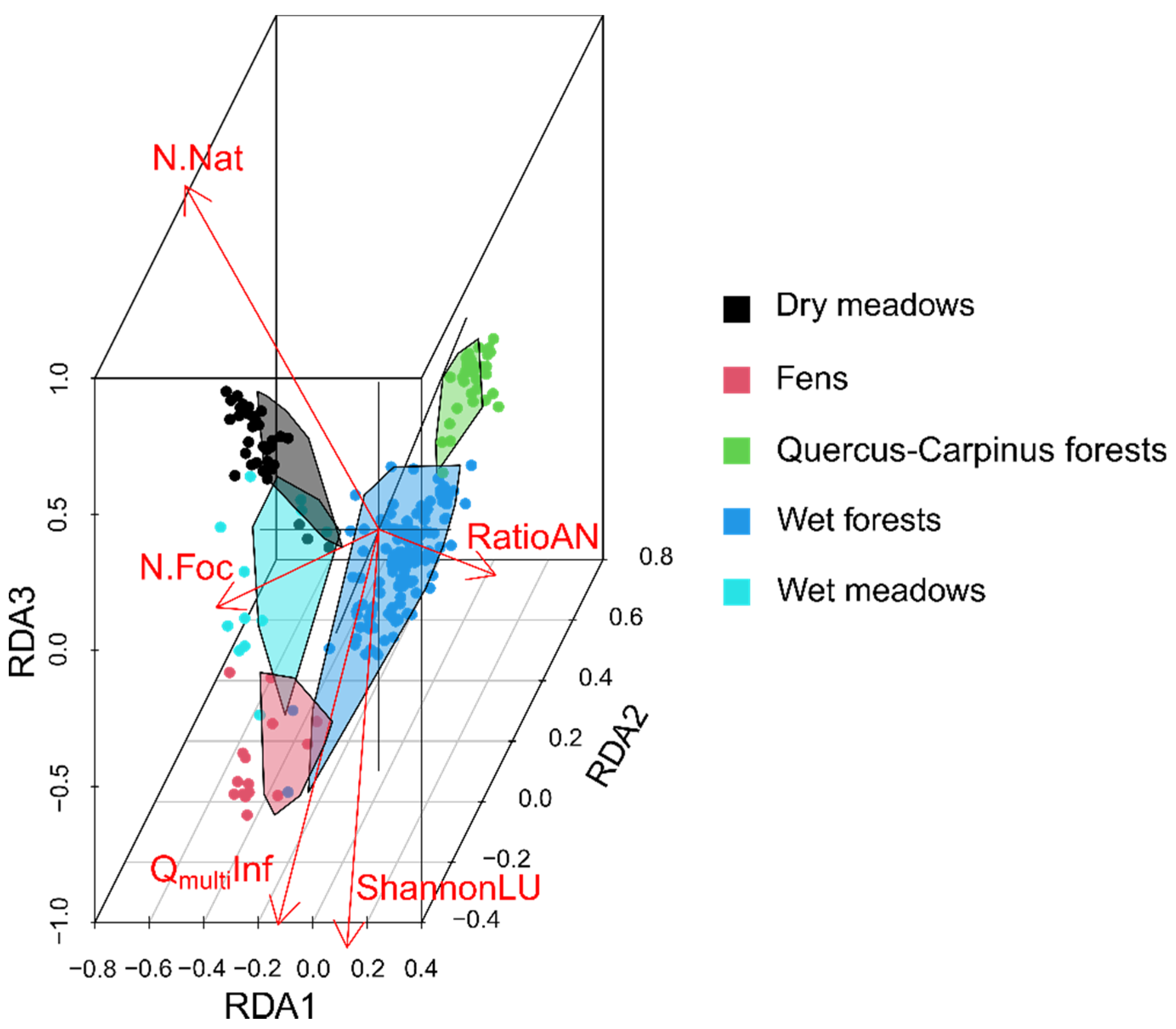
3.2. Spectral Heterogeneity vs. Landscape Heterogeneity and Taxonomic Plant Diversity

The resulting QNDVIInf and QmultiInf spectral heterogeneity maps, obtained from the “rasterdiv” package, are shown in Figure 3.
We observed significant relationships in all GAMs between spectral heterogeneity, land use diversity, and alien native species richness ratio, except for the term RatioAN in Qmulti1 GAM (Table 1, Figure S7). The adjusted R2 increased as the weight for the distance matrix was higher for both QNDVI and Qmulti GAMs. Comparing the models with the same distance weight, those with Qmulti always had a higher goodness-of-fit (Table 1). The best model (R2 = 0.43) was the one using the Qmulti with the highest distance weight. The linear term RatioAN was always positive related to Rao’s Q in all models, while the smooth term ShannonLU was more positively related to Rao’s Q the greater the distance weight considered (Figure S7).
The tb-RDA ordination explained 36.20% of the variance, the first three axes accounting for 11.30%, 10.15%, and 5.41% of the total explained variance, respectively (Figure 4). The first seven axes out of eighteen exceeded the threshold of statistical significance (p < 0.05). The first axis was correlated with native (N.Nat) and focal (N.Foc) species richness and ratio of alien to native species richness (RatioAN) and the second with land use diversity and spectral heterogeneity (ShannonLU and QmultiInf, Figure 4 and Figure S8). The axes from three to seven mainly described the difference between plant community composition in different habitats dictated by the presence of hygrophilous or xerophilous, woodland or grassland species. Forest habitats were mainly distributed along the second axis based on a gradient of spectral heterogeneity (RDA2 −0.54), land use diversity (RDA2 −0.44), and ratio of alien to native species richness (RDA2 −0.38) while fens and meadows were distributed on the first and third axes along a gradient of focal (RDA1 −0.40; RDA3 −0.38) and native species richness (RDA1 −0.37; RDA3 0.36). These gradients showed that higher values of Rao’s Q spectral heterogeneity were more related to wet habitats, and with those habitats where the land use diversity of the surrounding landscape was higher, features that are also known to often promote plant invasion.
The variance partitioning on species composition data highlighted that habitat was the main explanatory factor, accounting for 29% of the total variation (Figure S9). Interestingly, spectral heterogeneity and land use diversity contributed only to 8% of total variation, with the latter almost completely negligible in explaining plant community variations.

4. Discussion

This research aimed at investigating the use of SVH in a complex and anthropogenic landscape, using two new and promising methodological approaches for estimating α and β spectral diversity and ecosystem heterogeneity. Their outputs differed but both gave important information on plant diversity expendable for planning data collection and monitoring campaigns for biodiversity conservation programs.
The relationships between floristic and spectral α and β diversity indices provided evidence of the potential, but also of the limits, of remote sensing data as proxies of plant diversity [5]. In particular, in our case study, in a heterogeneous and anthropogenic landscape, where natural habitat patches (the nodes of the EN) are embedded in an agricultural matrix, these relationships were slightly weaker in comparison with other studies in homogeneous natural habitats [17,18,50,51,52,53,54]. For example, Féret and Asner [16], in homogeneous natural forests, reported a weak relationship between observed taxonomic and estimated spectral species richness that could be easily corrected with a linear factor derived from the relationship obtained between field data and estimation, as we also noticed in our results. Moreover, Féret and Asner [16] in tropical forests reported an underestimation of both α and β diversity indices but with high correlation rates (between 0.73 and 0.86 for α and between 0.61 and 0.75 for β). In contrast, we observed an overestimation of α diversity (H’) and an underestimation of β diversity (BC) and both diversity indexes achieved lower correlation values between floristic and spectral values (i.e., 0.53 and 0.48, respectively). However, considering the results from the averaged multiple images, we observed an underestimation of both indexes but with higher correlations between floristic and spectral values (i.e., 0.60 and 0.52, respectively). Our lower correlation values could derive, on one hand, from the lower relationship between spectral and taxonomic diversity observed by Rossi et al. [55] in grassland ecosystems. On the other hand, they may be determined by the plot dimension (10 m × 10 m) in comparison with that of the window used to calculate the spectral species (60 m × 60 m): in a highly heterogeneous landscape, such as the one under study, the signal can vary a lot moving away from the sampled plot due to plant community and land use variations, driven by many factor such as habitat type, anthropic pressure, landscape structure, and edge effects [56,57]. The effect of the grain size on the robustness in the relationship between spectral diversity and taxonomic diversity has been examined by different authors (e.g., [14,58]) and all of them concluded that the increase of the spatial scale of analysis, from both field and remotely sensed data, increased correlation between spectral heterogeneity and species richness. This issue, defined Modifiable Areal Unit Problem (MAUP), is a well-known pattern in landscape ecology and has been exhaustively discussed and analyzed by Jelinski and Wu [59]. This partly confirms that the performance of the spectral variability as a proxy of species diversity is influenced by the location and the extent of the reference region [60]. However, we found positive correlations between taxonomic and spectral diversity that could be applied, for example, for guiding sampling planning. Moreover, in our case, the relationship between taxonomic and spectral diversity values became more accurate for high diversity values (Figures S3–S6), thus highlighting that spectral diversity values become more reliable for biodiversity-rich areas that also represent the most important diversity hotspots to be monitored and preserved.
In addition, the spectral maps in Figure 2 have given evidence of the real differences between plots both in terms of α and β diversity. In fact, taking into consideration the entire study area and the sorting of the β diversity values of the pixels on the three axes of the PCoA (Figure 2c,d), it was possible to observe that the majority of the pixels linked to the positive part of the first axis of the sorting, represented in violet, corresponded to the forested nodes of the EN.
The results produced by “rasterdiv” package (Figure 3) highlighted the influence of the surrounding landscape composition and fragmentation on the values expressed by the Rao’s Q heterogeneity index. In fact, the areas with higher values of spectral heterogeneity were not those that we would expect to be richer in biodiversity, but those that were characterized by more anthropogenic impact (high values of land use diversity) and so also to biological invasion (high values of alien to native species richness ratio). Remote sensing data can provide information on complex systems, which depend on the original radiometric and spectral resolution, giving different results and interpretations depending on the composition of the study area and the type of existing vegetation. Using an ecological parallelism, the spectral space defined by many bands is analogous to the Hutchinson’s hypervolume, defined by a set of n independent axes corresponding to those variables (abiotic and biotic) shaping species’ niches [61,62]. In this case, spectral space was expected to be related to both species’ niches and their relative diversity [63], and this was the case, albeit with a relationship opposite to that expected. That is, greater spectral difference was found to be related to greater ratio of alien to native species richness rather than greater native or focal species richness (Figure 4). However, this result should not be neglected as it relates well to the use of remote sensing techniques for monitoring invasive alien plants across vast areas [64]. Many studies have demonstrated the capability of remote sensing approaches to detect invasive plant species and to map their distribution [65,66,67,68,69,70] and certainly the use of the Rao’s Q heterogeneity index in anthropogenic landscapes could be a powerful method to identify those areas potentially more prone to biological invasion.
GAMs (Table 1, Figure S7) showed that the greater the weighting between the spectral distance of pixels, the greater the relationship between spectral heterogeneity, land use diversity, and ratio of alien to native richness. It was interesting to observe that Qmulti was better explained than QNDVI by the above-mentioned variables, probably because the amount of spectral information contained in the 10 bands used in Qmulti was greater than that contained in the two bands of QNDVI, although the latter was calculated over a longer time frame. Spectral heterogeneity analysis suggests that the indexes can be interpreted in the opposite way (e.g., −Qmulti or −QNDVI) in our case study and could allow to identify a method to detect core areas within nodes (i.e., patches of natural habitats) of an EN. The core area is the inner part of a node that is less affected by the external impacts and to the edge effects. These latter are important ecological processes that are closely related to species habitat protection [71], community dynamics [72], and ecological restoration [73,74]. The analysis of heterogeneity using Rao’s Q can thus represent a new tool to be integrated in the context of EN structure optimization.
Variance partitioning (Figure S9) pointed out that the variable contributing the most to explaining differences among communities was habitat while the contribution of land use diversity is completely negligible in this context. Instead, spectral heterogeneity contributes to nearly one-third of the explained variation. This shows that the Rao’s Q in complex areas, not dominated by a single habitat, is unable to account for variation among different communities. However, this result also suggests, observing the forests in the ordination plot (Figure 4 and Figure S8), Rao’s Q potential to explain variation in the composition of the community in environments dominated by forest habitats.
Our results highlighted the effectiveness of estimating and mapping α and β spectral diversity and ecosystem spectral heterogeneity using remotely sensed images. This is currently a key topic in ecology and could provide landscape managers with rapid and effective tools to estimate and monitor global change [5]. Moreover, this study confirms once again the robustness and importance of SVH for estimating and monitoring diversity in different habitats [16,18,19,52,53,54]. In addition, we suggest experimenting with spectral heterogeneity analysis in the field of landscape ecology (e.g., ENs structure analysis) as well as the use of spectral diversity maps as fast approach in data-poor settings as starting base.
The observed relationship between spectral and floristic diversity, in a complex and anthropogenic landscape, supports SVH as a method to quickly estimate α and β diversity and heterogeneity. Moreover, it is suggested to explore their variation across regions to effectively implement monitoring and conservation plans allowing the production of maps for modeling and monitoring diversity from local to global scales [6,7,8].

5. Conclusions

The problem of quickly estimating the diversity and heterogeneity of a region to implement monitoring and conservation plans has a relevant impact on biodiversity management and natural resources conservation. Biodiversity assessment is today mainly performed by field survey, which is a time and cost-consuming method. This work explored the potential of SHV for estimating and monitoring diversity in an anthropogenic landscape, composed of different habitats. In this framework, two distinct methodological approaches for estimating α and β spectral diversity and ecosystem heterogeneity have been tested using the R packages “biodivMapR” and “rasterdiv”. These are based on different indices, but both are promising in the measurement of relationship between taxonomic diversity and spectral diversity. However, in heterogenous areas, they achieve lower correlation values between floristic and spectral values compared to the results obtained in areas characterized by extended and homogeneous natural landscapes, suggesting that spectral variability as a proxy of species diversity could be influenced both by the location characteristics (e.g., high or low landscape diversity, land use fragmentation) and by the extent of the reference regions. These aspects should be further explored. However, positive correlations between taxonomic and spectral diversity have been found, highlighting that spectral diversity values become more reliable for biodiversity-rich areas. The related thematic maps can contribute to informing processes of landscape management and planning. In fact, a fast method to discover biodiversity hotspots could support the detection of changes during a given time frame related to land use intensification/extensification or allow to address ground monitoring efforts on the potential biodiversity hot spots. Regarding the weaknesses of the two methods, in the case of “biodivMapR”, the possibility of working on time series would have to be implemented and the estimation of spectral species would have to be improved, which, as noted by the authors themselves, are always underestimated. In the case of “rasterdiv”, it would be appropriate to give different weight to radiometric variation depending on land use or discriminating between anthropogenic and natural areas.
Remote sensing data can provide information on complex systems, which depend on the original radiometric and spectral resolution, giving different results and interpretations depending on the composition of the study area and the type of existing vegetation. We found that this is true in particular in heterogeneous and anthropogenic landscapes where natural habitat patches are embedded in a heterogeneous agricultural matrix. This young research field needs further experimenting with both spectral diversity and spectral heterogeneity analysis to explore the potential of Sentinel-2A satellite data, available for free on ESA’s Sentinel Scientific Data Hub (https://scihub.copernicus.eu, accessed on 12 May 2022), which represent a powerful basis to map and monitor natural ecosystems.

Supplementary Materials

The following are available online at https://www.mdpi.com/article/10.3390/rs14194933/s1, Figure S1: Spectral diversity maps obtained from the analysis of the satellite image of 3 June 2019. Spectral α diversity map, expressed as Shannon index, of the study area (a) and of the EN nodes (b). Spectral β diversity map, expressed as Bray–Curtis dissimilarity index, produced by the projection of the n × n dimensional space of the dissimilarity matrix into an n × 3 dimensional space (PCoAs), of the study area (c) and of the EN nodes (d); Figure S2: Relationship between observed taxonomic and estimated spectral species richness unscaled (a) and scaled by 0.4 (b), using the single image (3 June 2019). The red line represents the relationship of 1 to 1; Figure S3: Relationship between observed taxonomic Shannon index (H’) and estimated spectral Shannon index (H’), using the single image (3 June 2019). The red line represents the relationship of 1 to 1; Figure S4: Relationship between observed taxonomic Bray–Curtis dissimilarity index (BC) and estimated spectral Bray–Curtis dissimilarity index (BC), using the single image (3 June 2019). The red line represents the relationship of 1 to 1; Figure S5: Relationship between observed taxonomic Shannon index (H’) and estimated spectral Shannon index (H’). The red line represents the relationship of 1 to 1; Figure S6: Relationship between observed taxonomic Bray–Curtis dissimilarity index (BC) and estimated spectral Bray–Curtis dissimilarity index (BC). The red line represents the relationship of 1 to 1; Figure S7: Relationships between spectral heterogeneity (Q), land use diversity (ShannonLU; smooth term), and alien to native species richness ratio (RatioAN; linear term), resulting from the six GAMs. Rao’s Q values derived from the NDVI time series (QNDVI) and the multispectral single image (Qmulti) and the weight for the distance matrix was set to 1, 5 and infinite; Figure S8: tb-RDA ordination based on Hellinger pre-transformed species composition matrix, with site grouped per habitat and displaying the following variables: focal species richness (N.Foc), native species richness (N.Nat), Rao’s Q index, calculated from the 10 bands of the Sentinel 2 image of 3 June 2019 with the weight for the distance matrix set to infinite (QmultiINF), and ratio of alien to native species richness (RatioAN), Shannon index on land use diversity (ShannonLU); Figure S9: Partition of the variation of the community matrix according to the three explanatory variable groups, namely habitat, land use heterogeneity, and spectral heterogeneity (Rao’s Q index); Table S1: Habitat of the area according to EUNIS habitat classification along with descriptive statistics of the study area (i.e., total area, mean area ± standard deviation, number of patches, number of plots and average total, native and alien richness).

Author Contributions

Conceptualization, F.L., M.S. and G.B.; methodology, F.L. and G.B.; formal analysis, F.L.; investigation, F.L.; data curation, F.L.; writing—original draft preparation, F.L.; writing—review and editing, M.S. and G.B.; supervision, M.S. and G.B. All authors have read and agreed to the published version of the manuscript.

Funding

This research received no external funding.

Data Availability Statement

Data presented in this study are available upon request to the corresponding author.

Conflicts of Interest

The authors declare no conflict of interest.

References

  1. IPBES. Summary for Policymakers of the Global Assessment Report on Biodiversity and Ecosystem Services of the Intergovernmental Science-Policy Platform on Biodiversity and Ecosystem Services; Díaz, S., Settele, J., Brondízio, E.S., Ngo, H.T., Guèze, M., Agard, J., Arneth, A., Balvanera, P., Brauman, K.A., Butchart, S.H.M., et al., Eds.; IPBES Secretariat: Bonn, Germany, 2019; 56p. [Google Scholar] [CrossRef]
  2. Vihervaara, P.; Auvinen, A.P.; Mononen, L.; Törmä, M.; Ahlroth, P.; Anttila, S.; Böttcher, K.; Forsius, M.; Heino, J.; Heliola, J.; et al. How essential biodiversity variables and remote sensing can help national biodiversity monitoring. Glob. Ecol. Conserv. 2017, 10, 43–59. [Google Scholar] [CrossRef]
  3. Yoccoz, N.G.; Nichols, J.D.; Boulinier, T. Monitoring of biological diversity in space and time. Trends Ecol. Evol. 2001, 16, 446–453. [Google Scholar] [CrossRef]
  4. Maccherini, S.; Bacaro, G.; Tordoni, E.; Bertacchi, A.; Castagnini, P.; Foggi, B.; Gennai, M.; Mugnai, M.; Sarmati, S.; Angiolini, C. Enough Is Enough? Searching for the Optimal Sample Size to Monitor European Habitats: A Case Study from Coastal Sand Dunes. Diversity 2020, 12, 138. [Google Scholar] [CrossRef] [Green Version]
  5. Rocchini, D.; Salvatori, N.; Beierkuhnlein, C.; Chiarucci, A.; de Boissieu, F.; Förster, M.; Garzon-Lopez, C.X.; Gillespie, T.W.; Hauffe, H.C.; He, K.S.; et al. From local spectral species to global spectral communities: A benchmark for ecosystem diversity estimate by remote sensing. Ecol. Inform. 2021, 61, 101195. [Google Scholar] [CrossRef]
  6. Féret, J.B.; Rocchini, D.; He, K.S.; Nagendra, H.; Luque, S. Forest species mapping. In A Sourcebook of Methods and Procedures for Monitoring Essential Biodiversity Variables in Tropical Forests with Remote Sensing; GOFC‐GOLD, GEO BON, Ed.; Report Version UNCBD COP-13 GOFC-GOLD Land Cover Project Office; Wageningen University: Wageningen, The Netherlands, 2017. [Google Scholar]
  7. Rocchini, D.; Boyd, D.S.; Féret, J.B.; Foody, G.M.; He, K.S.; Lausch, A.; Nagendra, H.; Wegmann, M.; Pettorelli, N. Satellite remote sensing to monitor species diversity: Potential and pitfalls. Remote Sens. Ecol. Conserv. 2016, 2, 25–36. [Google Scholar] [CrossRef]
  8. Rocchini, D.; Luque, S.; Pettorelli, N.; Bastin, L.; Doktor, D.; Faedi, N.; Feilhauer, H.; Féret, J.B.; Foody, G.M.; Gavish, Y.; et al. Measuring β-diversity by remote sensing: A challenge for biodiversity monitoring. Methods Ecol. Evol. 2018, 9, 1787–1798. [Google Scholar] [CrossRef] [Green Version]
  9. Féret, J.B.; de Boissieu, F. biodivMapR: An r package for α- and β-diversity mapping using remotely sensed images. Methods Ecol. Evol. 2020, 11, 64–70. [Google Scholar] [CrossRef]
  10. Rocchini, D.; Neteler, M. Let the four freedoms paradigm apply to ecology. Trends Ecol. Evol. 2012, 27, 310–311. [Google Scholar] [CrossRef]
  11. Palmer, M.W.; Earls, P.G.; Hoagland, B.W.; White, P.S.; Wohlgemuth, T. Quantitative tools for perfecting species lists. Environmetrics 2002, 13, 121–137. [Google Scholar] [CrossRef]
  12. Rocchini, D.; Hernández-Stefanoni, J.L.; He, K.S. Advancing species diversity estimate by remotely sensed proxies: A conceptual review. Ecol. Inform. 2015, 25, 22–28. [Google Scholar] [CrossRef]
  13. Lausch, A.; Heurich, M.; Magdon, P.; Rocchini, D.; Schulz, K.; Bumberger, J.; King, D.J. A Range of Earth Observation Techniques for Assessing Plant Diversity. In Remote Sensing of Plant Biodiversity, 1st ed.; Cavender-Bares, J., Gamon, J., Townsend, P., Eds.; Springer Nature: Cham, Switzerland, 2020; pp. 309–348. [Google Scholar]
  14. Rocchini, D.; Chiarucci, A.; Loiselle, S.A. Testing the spectral variation hypothesis by using satellite multispectral images. Acta Oecol. 2004, 26, 117–120. [Google Scholar] [CrossRef]
  15. Rocchini, D.; Balkenhol, N.; Carter, G.A.; Foody, G.M.; Gillespie, T.W.; He, K.S.; Kark, S.; Levin, N.; Lucas, K.; Luoto, M.; et al. Remotely sensed spectral heterogeneity as a proxy of species diversity: Recent advances and open challenges. Ecol. Inform. 2010, 5, 318–329. [Google Scholar] [CrossRef]
  16. Féret, J.B.; Asner, G.P. Mapping tropical forest canopy diversity using high-fidelity imaging spectroscopy. Ecol. Appl. 2014, 24, 1289–1296. [Google Scholar] [CrossRef] [PubMed] [Green Version]
  17. Heumann, B.W.; Hackett, R.A.; Monfils, A.K. Testing the spectral diversity hypothesis using spectroscopy data in a simulated wetland community. Ecol. Inform. 2015, 25, 29–34. [Google Scholar] [CrossRef]
  18. Torresani, M.; Rocchini, D.; Sonnenschein, R.; Zebisch, M.; Marcantonio, M.; Ricotta, C.; Tonon, G. Estimating tree species diversity from space in an alpine conifer forest: The Rao’s Q diversity index meets the spectral variation hypothesis. Ecol. Inform. 2019, 52, 26–34. [Google Scholar] [CrossRef] [Green Version]
  19. Marzialetti, F.; Cascone, S.; Frate, L.; Di Febbraro, M.; Acosta, A.T.R.; Carranza, M.L. Measuring Alpha and Beta Diversity by Field and Remote-Sensing Data: A Challenge for Coastal Dunes Biodiversity Monitoring. Remote Sens. 2021, 13, 1928. [Google Scholar] [CrossRef]
  20. Whittaker, R.H. Vegetation of the Siskiyou mountains, Oregon and California. Ecol. Monogr. 1960, 30, 279–338. [Google Scholar] [CrossRef]
  21. Whittaker, R.H. Evolution and measurement of species diversity. Taxon 1972, 21, 213–215. [Google Scholar] [CrossRef] [Green Version]
  22. Fahrig, L. Landscape heterogeneity and metapopulation dynamics. In Key Topics in Landscape Ecology; Wu, J., Hobbs, R., Eds.; Cambridge University Press: Cambridge, UK, 2007; pp. 78–91. [Google Scholar]
  23. Malanson, G.P.; Cramer, B.E. Landscape heterogeneity, connectivity, and critical landscapes for conservation. Divers. Distrib. 1999, 5, 27–39. [Google Scholar] [CrossRef]
  24. Lozier, J.D.; Strange, J.P.; Koch, J.B. Landscape heterogeneity predicts gene flow in a widespread polymorphic bumble bee, Bombus bifarius (Hymenoptera: Apidae). Conserv. Genet. 2013, 14, 1099–1110. [Google Scholar] [CrossRef]
  25. Marcantonio, M.; Iannacito, M.; Thouverai, E.; Da Re, D.; Tattoni, C.; Bacaro, G.; Vicario, S.; Ricotta, C.; Rocchini, D. rasterdiv: Diversity Indices for Numerical Matrices. 2021, R Package Version 0.2-3. Available online: https://CRAN.R-project.org/package=rasterdiv (accessed on 12 October 2021).
  26. Rocchini, D.; Thouverai, E.; Marcantonio, M.; Iannacito, M.; Da Re, D.; Torresani, M.; Bacaro, G.; Bazzichetto, M.; Bernardi, A.; Foody, G.M.; et al. rasterdiv—An Information Theory tailored R package for measuring ecosystem heterogeneity from space: To the origin and back. Methods Ecol. Evol. 2021, 12, 1093–1102. [Google Scholar] [CrossRef] [PubMed]
  27. Sigura, M.; Boscutti, F.; Buccheri, M.; Dorigo, L.; Glerean, P.; Lapini, L. La Rel dei Paesaggi di Pianura, di Area Montana e Urbanizzati. Piano Paesaggistico Regionale del Friuli-Venezia Giulia (Parte Strategica) E1 -Allegato alla Scheda di RER. Regione Friuli-Venezia Giulia. 2017. Available online: http://www.regione.fvg.it/rafvg/cms/RAFVG/ambiente-territorio/pianificazione-gestione-territorio/FOGLIA21/#id9 (accessed on 12 October 2021).
  28. Jones, T.A.; Hughes, J.M.R. Wetland inventories and wetland loss studies: A European perspective. In Waterfowl and Wetland Conservation in the 1990s: A Global Perspective, Proceedings of the IWRB Symposium, St Petersburg Beach, FL, USA, 12–19 November 1993; Moser, M., Prentice, R.C., van Vessem, J., Eds.; IWRB Spec. Publ. No. 26; IWRB: Slimbridge, UK, 1993; pp. 164–169. [Google Scholar]
  29. European Commission. Life and Europe’s Wetlands. Restoring a Vital Ecosystem; European Commission: Luxembourg, 2007.
  30. Jantke, K.; Schleupner, C.; Schneider, U.A. Gap analysis of European wetland species: Priority regions for expanding the Natura 2000 network. Biodivers. Conserv. 2011, 20, 581–605. [Google Scholar] [CrossRef]
  31. Liccari, F.; Castello, M.; Poldini, L.; Altobelli, A.; Tordoni, E.; Sigura, M.; Bacaro, G. Do Habitats Show a Different Invasibility Pattern by Alien Plant Species? A Test on a Wetland Protected Area. Diversity 2020, 12, 267. [Google Scholar] [CrossRef]
  32. Davies, C.E.; Moss, D.; Hill, M.O. EUNIS Habitat Classification Revised 2004; Report to the European Topic Centre on Nature Protection and Biodiversity; European Environment Agency: Copenhagen, Denmark, 2004.
  33. Chytrý, M.; Tichý, L.; Hennekens, S.M.; Knollová, I.; Janssen, J.A.M.; Rodwell, J.S.; Peterka, T.; Marcenò, C.; Landucci, F.; Danihelka, J.; et al. EUNIS habitat classification: Expert system, characteristic species combinations and distribution maps of European habitats. Appl. Veg. Sci. 2020, 23, 648–675. [Google Scholar] [CrossRef]
  34. Liccari, F.; Sigura, M.; Tordoni, E.; Boscutti, F.; Bacaro, G. Determining plant diversity within interconnected natural habitat remnants (ecological network) in an agricultural landscape: A matter of sampling design? Diversity 2022, 14, 12. [Google Scholar] [CrossRef]
  35. Liccari, F.; Boscutti, F.; Bacaro, G.; Sigura, M. Connectivity, landscape structure, and plant diversity across agricultural landscapes: Novel insight into effective ecological network planning. J. Environ. Manag. 2022, 317, 115358. [Google Scholar] [CrossRef]
  36. Bartolucci, F.; Peruzzi, L.; Galasso, G.; Albano, A.; Alessandrini, A.; Ardenghi, N.M.G.; Astuti, G.; Bacchetta, G.; Ballelli, S.; Banfi, E.; et al. An updated checklist of the vascular flora native to Italy. Plant. Biosyst. 2018, 152, 179–303. [Google Scholar] [CrossRef]
  37. Galasso, G.; Conti, F.; Peruzzi, L.; Ardenghi, N.M.G.; Banfi, E.; Celesti-Grapow, L.; Albano, A.; Alessandrini, A.; Bacchetta, G.; Ballelli, S.; et al. An updated checklist of the vascular flora alien to Italy. Plant. Biosyst. 2018, 152, 556–592. [Google Scholar] [CrossRef]
  38. Copernicus Open Access Hub. Sentinel-2 Data. Available online: https://scihub.copernicus.eu/ (accessed on 15 September 2021).
  39. SNAP-ESA Sentinel Application Platform v7.0. Available online: http://step.esa.int (accessed on 15 September 2021).
  40. Ustin, S.L.; Gamon, J.A. Remote sensing of plant functional types. New Phytol. 2010, 186, 795–816. [Google Scholar] [CrossRef]
  41. Homolová, L.; Malenovský, Z.; Clevers, J.G.P.W.; García-Santos, G.; Schaepman, M.E. Review of optical-based remote sensing for plant trait mapping. Ecol. Complex. 2013, 15, 1–16. [Google Scholar] [CrossRef] [Green Version]
  42. Shannon, C.E. A mathematical theory of communication. Bell. Syst. Tech. J. 1948, 23, 379–423. [Google Scholar] [CrossRef] [Green Version]
  43. Bray, J.R.; Curtis, J.T. An ordination of the upland forest communities of Southern Wisconsin. Ecol. Monogr. 1957, 27, 325–349. [Google Scholar] [CrossRef]
  44. Hamner, B.; Frasco, M. Metrics: Evaluation Metrics for Machine Learning. R package version 0.1.4. 2018. Available online: https://CRAN.R-project.org/package=Metrics (accessed on 12 October 2021).
  45. Rao, C.R. Diversity and dissimilarity coefficients: A unified approach. Theor. Popul. Biol. 1982, 21, 24–43. [Google Scholar] [CrossRef]
  46. Wood, S.N. Fast stable restricted maximum likelihood and marginal likelihood estimation of semiparametric generalized linear models. J. R. Stat. Soc. 2011, 73, 3–36. [Google Scholar] [CrossRef] [Green Version]
  47. Legendre, P.; Gallagher, E. Ecologically meaningful transformations for ordination of species data. Oecologia 2001, 129, 271–280. [Google Scholar] [CrossRef] [PubMed]
  48. Legendre, P.; Legendre, L. Numerical Ecology, 3rd ed.; Elsevier: Amsterdam, The Netherlands, 2012. [Google Scholar]
  49. Blanchet, F.G.; Legendre, P.; Bergeron, J.A.C.; He, F. Consensus RDA across dissimilarity coefficients for canonical ordination of community composition data. Ecol. Monogr. 2014, 84, 491–511. [Google Scholar] [CrossRef]
  50. Nagendra, H.; Rocchini, D.; Ghate, R.; Sharma, B.; Pareeth, S. Assessing plant diversity in a dry tropical forest: Comparing the utility of Landsat and Ikonos satellite images. Remote Sens. 2010, 2, 478–496. [Google Scholar] [CrossRef] [Green Version]
  51. Hall, K.; Reitalu, T.; Sykes, M.T.; Prentice, H.C. Spectral heterogeneity of QuickBird satellite data is related to fine-scale plant species spatial turnover in semi-natural grasslands. Appl. Veg. Sci. 2012, 15, 145–157. [Google Scholar] [CrossRef]
  52. Warren, S.D.; Alt, M.; Olson, K.D.; Irl, S.D.H.; Steinbauer, M.J.; Jentsch, A. The relationship between the spectral diversity of satellite imagery habitat heterogeneity, and plant species richness. Ecol. Inform. 2014, 24, 160–168. [Google Scholar] [CrossRef]
  53. Arekhi, M.; Yilmaz, O.Y.; Yilmaz, H.; Akyüz, Y.F. Can tree species diversity be assessed with Landsat data in a temperate forest? Environ. Monit. Assess. 2017, 189, 586. [Google Scholar] [CrossRef]
  54. Madonsela, S.; Cho, M.A.; Ramoelo, A.; Mutanga, O. Remote sensing of species diversity using Landsat 8 spectral variables. ISPRS J. Photogramm. 2017, 133, 116–127. [Google Scholar] [CrossRef] [Green Version]
  55. Rossi, C.; Kneubühler, M.; Schütz, M.; Schaepman, M.E.; Haller, R.M.; Risch, A.C. Spatial resolution, spectral metrics and biomass are key aspects in estimating plant species richness from spectral diversity in species-rich grasslands. Remote Sens. Ecol. Conserv. 2021, 8, 297–314. [Google Scholar] [CrossRef]
  56. Porensky, L.M.; Young, T.P. Edge-Effect Interactions in Fragmented and Patchy Landscapes. Conserv. Biol. 2013, 27, 509–519. [Google Scholar] [CrossRef] [PubMed]
  57. Amici, V.; Rocchini, D.; Filibeck, G.; Bacaro, G.; Santi, E.; Geri, F.; Landi, S.; Scoppola, A.; Chiarucci, A. Landscape structure effects on forest plant diversity at local scale: Exploring the role of spatial extent. Ecol. Complex. 2015, 21, 44–52. [Google Scholar] [CrossRef]
  58. Oldeland, J.; Wesuls, D.; Rocchini, D.; Schmidt, M.; Jurgens, N. Does using species abundance data improve estimates of species diversity from remotely sensed spectral heterogeneity? Ecol. Indic. 2010, 10, 390–396. [Google Scholar] [CrossRef]
  59. Jelinski, D.E.; Wu, J. The modifiable areal unit problem and implications for landscape ecology. Landsc. Ecol. 1996, 11, 129–140. [Google Scholar] [CrossRef]
  60. Schmidtlein, S.; Fassnacht, F.E. The spectral variability hypothesis does not hold across landscapes. Remote Sens. Environ. 2017, 192, 114–125. [Google Scholar] [CrossRef] [Green Version]
  61. Hutchinson, G. Homage to Santa Rosalia or why are there so many kinds of animals? Am. Nat. 1959, 93, 145–159. [Google Scholar] [CrossRef] [Green Version]
  62. Blonder, B. Hypervolume concepts in niche and trait based ecology. Ecography 2018, 41, 1441–1455. [Google Scholar] [CrossRef] [Green Version]
  63. Thouverai, E.; Marcantonio, M.; Bacaro, G.; Da Re, D.; Iannacito, M.; Marchetto, E.; Ricotta, C.; Tattoni, C.; Vicario, S.; Rocchini, D. Measuring diversity from space: A global view of the free and open source rasterdiv R package under a coding perspective. Community Ecol. 2021, 22, 1–11. [Google Scholar] [CrossRef]
  64. Rocchini, D.; Andreo, V.; Förster, M.; Garzon-Lopez, C.X.; Gutierrez, A.P.; Gillespie, T.W.; Hauffe, H.C.; He, K.S.; Kleinschmit, B.; Mairota, P.; et al. Potential of remote sensing to predict species invasions: A modelling perspective. Prog. Phys. Geogr. Earth Environ. 2015, 39, 283–309. [Google Scholar] [CrossRef] [Green Version]
  65. Müllerová, J.; Brůna, J.; Dvořák, P.; Bartaloš, T.; Vítková, M. Does the data resolution/origin matter? satellite, airborne and Uav imagery to tackle plant invasions. ISPRS—Int. Arch. Photogramm. Remote Sens. Spat. Inf. Sci. 2016, 41B7, 903–908. [Google Scholar] [CrossRef] [Green Version]
  66. Skowronek, S.; Asner, G.P.; Feilhauer, H. Performance of one-class classifiers for invasive species mapping using airborne imaging spectroscopy. Ecol. Inform. 2017, 37, 66–76. [Google Scholar] [CrossRef]
  67. Skowronek, S.; Ewald, M.; Isermann, M.; Kerchove, R.V.D.; Lenoir, J.; Aerts, R.; Warrie, J.; Hattab, T.; Honnay, O.; Schmidtlein, S.; et al. Mapping an invasive bryophyte species using hyperspectral remote sensing data. Biol. Invasions 2017, 19, 239–254. [Google Scholar] [CrossRef]
  68. Vaz, A.S.; Alcaraz-Segura, D.; Campos, J.C.; Vicente, J.R.; Honrado, J.P. Managing plant invasions through the lens of remote sensing: A review of progress and the way forward. Sci. Total Environ. 2018, 642, 1328–1339. [Google Scholar] [CrossRef]
  69. Lopatin, J.; Dolos, K.; Kattenborn, T.; Fassnacht, F.E. How canopy shadow affects invasive plant species classification in high spatial resolution remote sensing. Remote Sens. Ecol. Conserv. 2019, 5, 302–317. [Google Scholar] [CrossRef]
  70. Ewald, M.; Skowronek, S.; Aerts, R.; Lenoir, J.; Feilhauer, H.; Van De Kerchove, R.; Honnay, O.; Somers, B.; Garzón-López, C.X.; Rocchini, D.; et al. Assessing the impact of an invasive bryophyte on plant species richness using high resolution imaging spectroscopy. Ecol. Indic. 2020, 110, 105882. [Google Scholar] [CrossRef]
  71. Paton, P. The effect of edge on avian nest success: How strong is the evidence? Conserv. Biol. 1994, 8, 17–26. [Google Scholar] [CrossRef]
  72. Fagan, W.; Cantrell, R.; Cosner, C. How habitat edges change species interaction. Am. Nat. 1999, 153, 165–182. [Google Scholar] [CrossRef]
  73. Loveridge, A.; Hemson, G.; Davidson, Z.; Macdonald, D. African lions on the edge: Reserve boundaries as “attractive sinks”. Biol. Conserv. Wild Felids 2010, 283, 283–304. [Google Scholar]
  74. An, Y.; Liu, S.; Sun, Y.; Beazley, R. Construction and optimization of an ecological network based on morphological spatial pattern analysis and circuit theory. Landsc. Ecol. 2021, 36, 2059–2076. [Google Scholar] [CrossRef]
Figure 1. Location of the study area (red square) in relation to the European continent (top right). Representation of the Ecological Network model and location of sampling units within the study area (main figure). Colored lines and patches are corridors and nodes of the network, representing different habitat types and species-specific networks. EUNIS Habitat Codes are as follows: D4.11 Schoenus nigricans fens; D5.24 Fen Cladium mariscus beds; E1.55 Eastern sub-Mediterranean dry grassland; E2.2 Low and medium altitude hay meadows; E3.51 Molinia caerulea meadows and related communities; G1.A1A Illyrian Quercus-Carpinus betulus forests; G1.11 Riverine Salix woodland; G1.22 Southeast European Fraxinus-Quercus-Alnus forests; G1.41 Alnus swamp woods not on acid peat.
Remotesensing 14 04933 g001
Figure 2. Spectral α diversity map, expressed as Shannon index (H’), of the study area (a) and of the EN nodes (b). Spectral β diversity map, expressed as Bray–Curtis dissimilarity index (BC), produced by the projection of the n × n dimensional space of the dissimilarity matrix into an n × 3 dimensional space (PCoAs), of the study area (c) and of the EN nodes (d). Similar colors, resulting from the PCoA ordination, represent similar spectral plant communities.
Remotesensing 14 04933 g002
Figure 3. Rao’s Q index, calculated from the NDVI time series covering the year 2019 (QNDVI) with the weight for the distance matrix set to infinite, for the study area (a). Rao’s Q index, calculated from the 10 bands of the Sentinel 2 image of 3 June 2019 (Qmulti) with the weight for the distance matrix set to infinite, for the study area (b).
Remotesensing 14 04933 g003
Figure 4. tb-RDA ordination based on Hellinger pre-transformed species composition matrix, with site grouped per habitat and displaying the following variables: focal species richness (N.Foc), native species richness (N.Nat), Rao’s Q index, calculated from the 10 bands of the Sentinel 2 image of 3 June 2019 with the weight for the distance matrix set to infinite (QmultiINF), and ratio of alien to native species richness (RatioAN), Shannon index on land use diversity (ShannonLU).
Remotesensing 14 04933 g004
Table 1. Summary of generalized additive models (GAMs) for spectral heterogeneity (Rao’s Q index calculated from NDVI timeseries (QNDVI) and from a multispectral image (Qmulti) with three different weights for the distance matrix (i.e., 1, 5, infinite) vs. alien native species richness ratio (RatioAN, linear term) and Shannon index calculated on land uses (ShannonLU, smooth term). Est. ± SE = estimate ± standard error; Edf = effective degrees of freedom.
QNDVI1 ~ RatioAN + s(ShannonLU)Est. ± SEp-ValueEdfR2 = 0.21
Termsp-Value
Intercept45.43 ± 1.95<0.001--
RatioAN51.82 ± 19.830.010--
Smooth (ShannonLU)--2.25<0.001
QNDVI5 ~ RatioAN + s(ShannonLU) R2 = 0.25
Intercept76.36 ± 3.49<0.001--
RatioAN99.34 ± 35.600.006--
Smooth (ShannonLU)--3.37<0.001
QNDVIInf ~ RatioAN + s(ShannonLU) R2 = 0.27
Intercept282.50 ± 12.34<0.001--
RatioAN347.65 ± 125.880.006--
Smooth (ShannonLU)--3.67<0.001
Qmulti1 ~ RatioAN + s(ShannonLU) R2 = 0.25
Intercept51.92 ± 1.59<0.001--
RatioAN18.02 ± 16.20NS--
Smooth (ShannonLU)--3.34< 0.001
Qmulti5 ~ RatioAN + s(ShannonLU) R2 = 0.41
Intercept92.52 ± 2.40<0.001--
RatioAN72.55 ± 24.550.003--
Smooth (ShannonLU)--4.64<0.001
QmultiInf ~ RatioAN + s(ShannonLU) R2 = 0.43
Intercept368.62 ± 9.64<0.001--
RatioAN401.20 ± 98.43<0.001--
Smooth (ShannonLU)--4.51<0.001
Publisher’s Note: MDPI stays neutral with regard to jurisdictional claims in published maps and institutional affiliations.

