Comparison of S5P/TROPOMI Inferred NO₂ Surface Concentrations with In Situ Measurements over Central Europe

Abstract

The aim of this paper is to evaluate the surface concentration of nitrogen dioxide (NO₂) inferred from the Sentinel-5 Precursor Tropospheric Monitoring Instrument (S5P/TROPOMI) NO₂ tropospheric column densities over Central Europe for two time periods, summer 2019 and winter 2019–2020. Simulations of the NO₂ tropospheric vertical column densities and surface concentrations from the Long-Term Ozone Simulation–European Operational Smog (LOTOS-EUROS) chemical transport model are also applied in the methodology. More than two hundred in situ air quality monitoring stations, reporting to the European Environment Agency (EEA) air quality database, are used to carry out comparisons with the model simulations and the spaceborne inferred surface concentrations. Stations are separated into seven types (urban traffic, suburban traffic, urban background, suburban background, rural background, suburban industrial and rural industrial) in order to examine the strengths and shortcomings of the different air quality markers, namely the NO₂ vertical column densities and NO₂ surface concentrations. S5P/TROPOMI NO₂ surface concentrations are inferred by multiplying the fraction of the satellite and model NO₂ vertical column densities with the model surface concentrations. The estimated inferred TROPOMI NO₂ surface concentrations are examined further with the altering of three influencing factors: the model vertical leveling scheme, the versions of the TROPOMI NO₂ data and the air mass factors applied to the satellite and model NO₂ vertical column densities. Overall, the inferred TROPOMI NO₂ surface concentrations show a better correlation with the in situ measurements for both time periods and all station types, especially for the industrial stations (R > 0.6) in winter. The calculated correlation for background stations is moderate for both periods (R~0.5 in summer and R > 0.5 in winter), whereas for traffic stations it improves in the winter (from 0.20 to 0.50). After the implementation of the air mass factors from the local model, the bias is significantly reduced for most of the station types, especially in winter for the background stations, ranging from +0.49% for the urban background to +10.37% for the rural background stations. The mean relative bias in winter between the inferred S5P/TROPOMI NO₂ surface concentrations and the ground-based measurements for industrial stations is about −15%, whereas for traffic urban stations it is approximately −25%. In summer, biases are generally higher for all station types, especially for the traffic stations (~−75%), ranging from −54% to −30% for the background and industrial stations.

1. Introduction

Nitrogen oxides (NO_X = NO + NO₂) play a significant role in tropospheric chemistry and have a negative impact on air quality. Nitrogen dioxide (NO₂) is a precursor of tropospheric ozone and aerosols [1,2,3] and has been associated with premature deaths and high mortality rates [4,5]. The short lifetime and the high spatial variability of NO₂ emission sources traditionally limited the spatial representativity of monitoring of NO₂ loads in non-background locations with in situ measurements only. The quantification of the spatial variability of NO₂ concentrations from satellite observations bridges this spatial gap. There are multiple satellite instruments providing spaceborne measurements that are able to detect emission sources at high spatiotemporal resolution on a global scale and are used to develop methods for estimating NO₂ surface concentrations and improving forecasting models [6].

Previous studies directly compared satellite NO₂ vertical column densities with ground-based measurements over Helsinki and have shown a mean relative bias of 10% [7], while a strong spatial correlation (R = 0.8) is reported over the USA [8]. Because of the limited number of ground-based stations and the fact that NO₂ satellite columns are not truly representing ground-level measurements, new methodologies were developed aiming to derive NO₂ surface concentrations from satellite vertical column densities with the use of chemical transport models [9,10,11,12,13,14,15,16]. In particular, a high correlation coefficient (up to 0.86) was reported between satellite-derived NO₂ surface concentrations and ground-based measurements, with a tendency for higher correlations over polluted areas, in northern USA [9]. Satellite-derived NO₂ surface concentration trends for the period 1996–2012 have shown decreasing NO₂ loads over North America, western Europe and Asia-Pacific, and were found to be highly correlated with in situ measurements especially over non-rural areas (R~0.8) [12]. Moreover, inferred satellite NO₂ surface concentrations reported improved correlation coefficients with ground-based measurements over China compared to the correlation coefficients calculated between forward model simulations and in situ measurements [14]. A new algorithm for the derivation of satellite NO₂ surface concentrations has shown a significant improvement in the correlation coefficients between the Sentinel-5 Precursor Tropospheric Monitoring Instrument (S5P/TROPOMI) inferred concentrations and ground-based observations [15,16]. More recently, machine learning techniques have been developed for the derivation of satellite NO₂ surface concentrations, which show promising results [17,18,19]. Hence, it is evident that the derivation of NO₂ surface concentrations from satellite observations has introduced new capabilities in the monitoring of air quality at the ground, contributing to the implementation of emission-reduction strategies and the development of health studies.

In this work, NO₂ surface concentrations are derived from TROPOMI NO₂ tropospheric vertical column densities (VCDs) and Long-Term Ozone Simulation–European Operational Smog (LOTOS-EUROS) chemical transport model (CTM) simulations following the methodology described in [9]. The inferred TROPOMI NO₂ surface concentrations are validated with in situ measurements reported by the European Environment Agency (EEA) stations over central Europe and for two studied periods, June–July 2019 and December 2019–January 2020. Three different setups are applied for estimating the satellite NO₂ surface concentrations and the results are examined based on three influencing quantities, namely the vertical leveling scheme of the LOTOS-EUROS CTM, the product version of the TROPOMI NO₂ data and the air mass factors (AMFs) used in each setup. This study is structured as follows. In Section 2, all the involved datasets are described in detail and the methodology is presented. In Section 3.1, the results are presented, and the impacts of the tested influencing factors are discussed. Section 3.2 presents the optimal setup used in this work. Finally, Section 4 summarizes the main findings of this study.

2. Materials and Methods

2.1. Datasets

2.1.1. S5P/TROPOMI NO₂ Tropospheric Vertical Column Densities

The Tropospheric Monitoring Instrument (TROPOMI) is a passive, nadir-viewing spectrometer onboard the European Space Agency (ESA) Sentinel-5 Precursor (S5P) satellite [20], launched during October 2017. TROPOMI provides measurements of various trace gas columns, aerosol, and cloud properties in four channels (UV, visible, IR and SWIR) with a very high spatial resolution of 3.5 km² × 7 km² (3.5 km² × 5.5 km² as of August 2019), from an ascending sun-synchronous polar orbit [21,22,23]. The high spatial resolution combined with an improved signal-to-noise ratio compared to previous spaceborne instruments allows the detection of local anthropogenic emission sources [8,24,25,26]. The tropospheric NO₂ VCD retrieval is performed in the 405–465 nm range. TROPOMI data are generated with the DOMINO (Dutch OMI NO₂) algorithm, which is also used for the Ozone Monitoring Instrument (OMI) data production [27,28]. Details concerning the standard operational NO₂ product can be found in the Algorithm Theoretical Basis Document [22] and the Product User Manual [29].

In this work, we use offline v1.3 and v2.3 S5P/TROPOMI tropospheric vertical column densities (VCDs) for two sensing periods (June–July 2019 and December 2019–January 2020). According to the latest validation report [30], a mean negative bias of −32% is found in the tropospheric column densities between TROPOMI v1.3 and MAX-DOAS ground-based data from 27 stations. The bias depends on the pollution level at the station, being positive over clean areas (18%) and negative (−46%) over highly polluted areas, but overall within the mission requirement of 50%. The low TROPOMI tropospheric VCDs over highly polluted areas have led to the implementation of improvements in the TROPOMI NO₂ retrieval algorithm leading to version 2.3. The new TROPOMI v2.3 data, publicly available via the ESA Sentinel-5P Product Algorithm Laboratory (S5P-PAL) show, on average, higher tropospheric VCDs up to 10–40% compared to the v1.3 data, depending on the level of pollution and season, especially in winter over mid and high latitudes [23]. Comparisons with ground-based data show that v2.3 TROPOMI data reduces the mean bias of the tropospheric columns from −32% to −23%, the stratospheric from −6% to −3% and the total column bias from −12% to −5%, respectively [23].

For the purposes of this study, we use observations of scenes that are mostly cloud-free with an associated quality flag higher than 0.75. The daily orbital files for the sensing periods are gridded onto a 0.05° × 0.1° grid covering the European domain. Figure 1 depicts the TROPOMI v1.3 (Figure 1a) and v2.3 (Figure 1b) tropospheric VCDs for December 2019 and their differences (Figure 1c). The same maps for June 2019 are shown in Figure A1. The v2.3 columns show higher values (by 16% on average) over highly polluted areas, namely the Po valley in northern Italy, the cities of Essen, Dusseldorf and Koln in western Germany and the cities of Rotterdam, Brussels and Paris. The differences are more pronounced in winter, whereas slightly higher NO₂ VCDs in v1.3 TROPOMI data are observed over a handful of rural and background areas located in central Germany. More specifically, the TROPOMI v2.3 tropospheric VCDs are about 3% higher in June and July compared to the v1.3 dataset, whereas in winter, v2.3 data are by 11–18% higher for the whole domain. Over the hotspots mentioned above, the bias is approximately 13% in summer and ranges between 16–26% in winter, as reported in [23].

2.1.2. LOTOS-EUROS CTM Simulations

In this work, the LOTOS-EUROS chemical transport model is used [31]. LOTOS-EUROS is one of the nine state-of-the-art models used in the Copernicus Atmosphere Monitoring Service (CAMS) to provide air quality forecasts to a broad range of users. It simulates distinct components (e.g., oxidants, primary aerosol, heavy metals) in three dimensions in the lower atmosphere [32]. The model has been used in a wide range of air quality studies and has been extensively evaluated against in situ measurements. A model evaluation against ground-based measurements over two major Greek cities has shown that the modeled NO₂ surface concentrations show a high spatial correlation of 0.86 and a moderate underestimation of about 10% [33]. When compared to industrial stations located near power plants in Greece, LOTOS-EUROS NO₂ surface concentrations mean seasonal bias improves to 2 μg/m³ from 10 μg/m³, after assimilating the spaceborne TROPOMI NO₂ observations [34]. The model has also been recently used to estimate changes in NO₂ emissions due to the COVID-19 pandemic restrictive measures [26] and to study NO₂ concentrations attributed to shipping activity in the Mediterranean and the Black Sea basin [35]. Both studies show significant agreement with TROPOMI satellite observations (R~0.95).

For this study, we use the LOTOS-EUROS v2.02.001 open-source version and more specifically the NO₂ tropospheric vertical column densities and NO₂ surface concentrations over the central European domain and selected pixels representative of the ground-based station locations. A nested domain configuration was used. Two model runs with different spatial resolutions were performed to maximize the smooth transition of dynamics between a coarser European domain and a refined central European domain. The first (outer) run covers the European domain from 15° W to 45° E and from 30° N to 60° N with a horizontal resolution of 0.25° × 0.25°. Boundary and initial conditions of this run are obtained from the CAMS global near-real-time (NRT) product with a spatial resolution of 35 km × 35 km. The second (inner) run was performed for central Europe, from 2° E to 18° E and from 39° N to 55° N with a horizontal resolution of 0.05° × 0.10° (latitude x longitude). Boundary conditions of the inner run are obtained from the lower resolution outer domain. The model simulations are driven by operational meteorological data from the European Centre for Medium-Range Weather Forecasts (ECMWF) with a horizontal resolution of 7 km × 7 km [36]. Finally, the CAMS-REG (CAMS regional European emissions) v4.2 for the year 2017 available at 0.05° × 0.10° [37] is the anthropogenic emission inventory used in the model.

2.1.3. CAMS Satellite Operator (CSO)

The CAMS Satellite Operator (CSO, https://ci.tno.nl/gitlab/cams/cso, last accessed 30 June 2022) is a toolbox to facilitate assimilation of satellite observations in regional air quality models. It contains two main entities: a preprocessor that can be used to download and convert satellite data, in particular TROPOMI data, and an observation operator that can be added to the source code of a model simulation. With this operator, the module can perform simulations of the satellite retrievals and use them in a data assimilation procedure. The observation operator is included in the LOTOS-EUROS source code, and it is used to provide simulations, as described below.

More specifically, the TROPOMI tropospheric NO₂ retrieval product (y_r) is treated by CSO as a profile with one layer from the surface up to 200 hPa. The simulation of a retrieval product from a model state does not require an a priori profile and is denoted with:

y_s = A^trop ∗ H ∗ x

(1)

where:

• y_s is the simulated retrieval defined on a single layer profile, n_r = 1;
• A^trop is the tropospheric averaging kernel with shape (n_r, n_a); in this product n_a = 34, the number of a priori layers covering the full atmosphere;
• X is a concentration profile defined on model layers covering the full atmosphere; values above 200 hPa are actually ignored;
• H extracts a simulated profile from the model using vertical and horizontal interpolation.

The tropospheric averaging kernel is derived from Equation (2):

$$\begin{gathered} {\mathrm{A}}^{\mathrm{trop}}[:,\mathrm{l}]=\frac{\mathrm{M}}{{\mathrm{M}}^{\mathrm{trop}}[:]} \ast \mathrm{A}[:,\mathrm{l}], \mathrm{l} \le {\mathrm{l}}_{\mathrm{tp}} \\ {\mathrm{A}}^{\mathrm{trop}}[:,\mathrm{l}]=0, 1 \ge {\mathrm{l}}_{\mathrm{tp}} \end{gathered}$$

(2)

using the following entities from the retrieval product:

• A is the total column averaging kernel;
• M is the scalar total column air mass factor;
• M^trop is the tropospheric column air mass factor;
• l_tp is the index of the layer containing the tropopause in the a priori profile.

The air mass factors in the TROPOMI product are based on simulations with the TM5-MP global atmospheric model [38] at the coarser resolution of 0.5° × 0.5°. Thus, the air mass factors do not represent the strong gradients near high emitting sources. This can be improved by replacing the original tropospheric averaging kernels of the retrieval, depending on the a priori profiles of the TM5-MP model, with the LOTOS-EUROS higher resolution model profiles. As described in [29], the first step is to estimate an alternative tropospheric air mass factor using the alternative a priori profile (${\widehat{x}}_a$), in our case a LOTOS-EUROS simulation:

$${\hat{\mathrm{M}}}^{\mathrm{trop}}({\hat{\mathrm{x}}}_{\mathrm{a}})= {\mathrm{M}}^{\mathrm{trop}} \ast ({\mathrm{A}}^{\mathrm{trop}} \ast \mathrm{H} \ast {\hat{\mathrm{x}}}_{\mathrm{a}})/({\sum }_{\mathrm{l}=1}^{\mathrm{ltp}}{(\mathrm{H} \ast {\hat{\mathrm{x}}}_{\mathrm{a}})}_{\mathrm{l}}$$

(3)

This is used to obtain the updated retrieval and tropospheric averaging kernel as scaled versions of the original variables, as described in Equations (4) and (5).

$${\hat{\mathrm{y}}}_{\mathrm{r}}({\hat{\mathrm{x}}}_{\mathrm{a}})=({\mathrm{M}}^{\mathrm{trop}}/{\hat{\mathrm{M}}}^{\mathrm{trop}}({\hat{\mathrm{x}}}_{\mathrm{a}})) \ast {\mathrm{y}}^{\mathrm{r}}$$

(4)

$${\hat{\mathrm{A}}}^{\mathrm{trop}} ({\hat{\mathrm{x}}}_{\mathrm{a}})=({\mathrm{M}}^{\mathrm{trop}}/{\hat{\mathrm{M}}}^{\mathrm{trop}}({\hat{\mathrm{x}}}_{\mathrm{a}})) \ast {\mathrm{A}}^{\mathrm{trop}}$$

(5)

Thus, the new simulations can be estimated by replacing the variables in Equation (1), initially with Equation (5) and then with Equation (3).

$$\begin{gathered} {\hat{\mathrm{y}}}_{\mathrm{s}}({\hat{\mathrm{x}}}_{\mathrm{a}})={\hat{\mathrm{A}}}^{\mathrm{trop}} ({\hat{\mathrm{x}}}_{\mathrm{a}}{)}^{ }\ast \mathrm{H} \ast {\hat{\mathrm{x}}}_{\mathrm{a}} \\ =({\mathrm{M}}^{\mathrm{trop}}/{\hat{\mathrm{M}}}^{\mathrm{trop}}({\hat{\mathrm{x}}}_{\mathrm{a}})) \ast {\mathrm{A}}^{\mathrm{trop}} \ast \mathrm{H} \ast {\hat{\mathrm{x}}}_{\mathrm{a}} \\ =\frac{{\mathrm{M}}^{\mathrm{trop}}}{{\mathrm{M}}^{\mathrm{trop}}({\mathrm{A}}^{\mathrm{trop}} \ast \mathrm{H} \ast {\hat{\mathrm{x}}}_{\mathrm{a}})/({\sum }_{\mathrm{l}=1}^{\mathrm{ltp}}{(\mathrm{H} \ast {\hat{\mathrm{x}}}_{\mathrm{a}})}_{\mathrm{l}})} {\mathrm{A}}^{\mathrm{trop}} \ast \mathrm{H} \ast {\hat{\mathrm{x}}}_{\mathrm{a}} \\ =({\sum }_{\mathrm{l}=1}^{\mathrm{ltp}}{(\mathrm{H}\ast {\hat{\mathrm{x}}}_{\mathrm{a}})}_{\mathrm{l}}) \end{gathered}$$

(6)

The effect of the aforementioned process is illustrated in Figure 2. Figure 2a shows the original TROPOMI v2.3 NO₂ VCDs, while Figure 2b depicts the TROPOMI v2.3 NO₂ VCDs after the application of the local air mass factor correction described in Equations (4) and (5). Figure 2c shows the differences between those two datasets for December 2019. The updated TROPOMI v2.3 NO₂ VCDs with the local air mass factor correction show sharper gradients, especially over highly polluted areas in western Germany, the Netherlands, Belgium, the Po valley, and cities such as Paris, Rome and Naples. Increased NO₂ concentrations can also be observed over rural and background areas in central Germany and eastern France. Over the whole domain, the updated NO₂ VCDs are higher by approximately 20% when compared to the original NO₂ VCDs. Over hotspots, the updated TROPOMI v2.3 NO₂ VCDs show higher levels by approximately 18% for both periods, while over rural areas concentrations are higher by 16% and 22% for the summer and winter, respectively.

Note that assimilation is not applied for the purposes of this study. The NO₂ products from the CSO process are used as input for the estimation of TROPOMI inferred NO₂ surface concentrations, as described in detail in the methodology.

2.1.4. European Environmental Agency In Situ Measurements

Hourly in situ measurements of NO₂ surface concentrations over central Europe are obtained from the European Environment Agency (EEA) (https://discomap.eea.europa.eu/map/fme/AirQualityExport.htm, last accessed on 11 July 2022). The European air quality database includes information concerning the monitoring of air quality from all member countries of the European Union (EU) and additionally some countries that cooperate with the EEA. This dataset is used for the evaluation of the satellite-derived NO₂ surface concentrations and the LOTOS-EUROS simulations. In situ measurements at 11:00 UTC were chosen as representative of the overpass time of S5P for June, July, December 2019 and January 2020.

For this work, data from 236 stations were used for over 20 locations in central Europe (Figure 3). The choice of the station location was not arbitrary and specific criteria were considered. The stations had to be distributed all over the domain, thus comparisons could be made for various regions and area types (traffic, background, rural, etc.). The stations are categorized in the EEA database in the following types: urban traffic (81), suburban traffic (7), urban background (86), suburban background (30), rural background (19), suburban industrial (6) and rural industrial (7).

2.2. Methodology

The objective of this work is to estimate NO₂ surface concentrations inferred from S5P/TROPOMI NO₂ tropospheric VCDs using as input LOTOS-EUROS CTM simulations. The basis of the methodology is described by Equation (7), originally applied in [9]. According to Equation (7), the derived NO₂ satellite concentrations are equal to the fraction of the NO₂ VCDs of the satellite and the chemical transport model multiplied by the surface concentration of the lowest vertical layer of the model.

S_o = (Ω_O/Ω_G) ∗ S_G

(7)

where:

• S_o, inferred TROPOMI NO₂ surface concentration;
• S_G, NO₂ surface concentration of the model;
• Ω_G, NO₂ tropospheric VCDs of the model;
• Ω_ο, NO₂ tropospheric VCDs from the satellite observations.

The model vertical profiles are obtained for 11:00 UTC, corresponding to the closest time of the TROPOMI overpass across the domain. Three surface datasets are estimated based on three different setups involving the various datasets of the simulations and the satellite retrievals. More specifically, the first dataset of the inferred TROPOMI NO₂ surface concentrations is derived by using as input the TROPOMI NO₂ tropospheric VCDs and the a priori LOTOS-EUROS NO₂ tropospheric VCDs and surface concentrations. The second dataset includes the CSO simulations where the TM5-MP averaging kernels are applied to the LOTOS-EUROS vertical profiles. Finally, the third dataset is derived by applying the satellite and model NO₂ VCDs, updated with the new air mass factors and averaging kernels, and the a priori LOTOS-EUROS NO₂ surface concentrations to Equation (7).

Table 1. Datasets and their products involved in each setup in order to estimate TROPOMI inferred NO₂ surface concentrations.

Datasets	Setup 1/Baseline	Setup 2	Setup 3
LOTOS-EUROS	A priori NO2 surface concentrations and a priori NO2 VCDs	NO2 surface concentrations and NO2 VCDs with TM5-MP AKs	A priori NO2 surface concentrations and NO2 VCDs with updated AMFs and AKs
TROPOMI	Original NO2 VCD	Original NO2 VCD	NO2 VCD with updated AMFs and AKs
Surface products	TROPOMI inferred NO2 surface concentration	TROPOMI inferred NO2 surface concentrations with TM5-MP AKs	TROPOMI inferred NO2 surface concentrations with model air mass factors correction

describes the model and satellite datasets used in each setup applied to the methodology to derive the inferred NO₂ satellite surface concentrations products, as discussed above.

The modeled and inferred TROPOMI NO₂ surface concentrations of the closest pixels to the station locations are selected to carry out comparisons with the EEA in situ measurements. To ease the understanding of the process, we provide here a first example of the results, which are discussed in detail further on. Figure 4 shows the derived satellite NO₂ surface concentrations (in μg/m³) for July 2019 (left column) and for January 2020 (right column) based on the three setups shown in Table 1. Figure 4a,b depict the inferred TROPOMI v2.3 NO₂ surface concentrations of the first setup with the original TROPOMI v2.3 product and the a priori LOTOS-EUROS simulations. Figure 4c,d show the second setup of inferred NO₂ surface concentrations with the inclusion of the CSO simulations and the application of the TM5-MP averaging kernels on the LOTOS-EUROS profiles. Finally, Figure 4e,f illustrate the third setup of the estimated NO₂ satellite surface concentrations with the updated averaging kernels (AKs) and air mass factors. It is evident that as we move from the case of not applying AKs (Figure 4a,b), to applying the original TROPOMI TM5-MP AKs (Figure 4c,d) and to applying the updated CSO AKs (Figure 4e,f), the inferred NO₂ surface concentration increases, for both time periods. The road transport and shipping emitting lanes appear clearly in the second and third setups, even more pronounced in the third setup for the month of July in the Po valley and the Adriatic Sea. For January 2020, the third setup shows overall higher NO₂ concentrations, as expected, compared to the other two setups, and sharper gradients in the vicinity of the highs of the Po valley and southern Germany.

3. Results

3.1. Investigation into Influencing Quantities

In this section, the most prominent quantities that affect the methodology are studied and the results are analyzed. The aim of the derivation of satellite NO₂ surface concentrations is mainly to provide information at locations where ground-based stations do not exist. Therefore, each quantity involved needs to be studied in detail and cross-validated with in situ measurements. Three instances and their imprint on the results are examined: the vertical levelling scheme used in the LOTOS-EUROS CTM and the CSO operator simulations (Section 3.1.1), the versions of the S5P/TROPOMI satellite data (Section 3.1.2), and the new updated air mass factors estimated through the CSO process (Section 3.1.3).

3.1.1. LOTOS-EUROS Vertical Leveling Scheme

Initially, the effect of the LOTOS-EUROS CTM vertical leveling scheme on the results is examined. There are three methods to define vertical layers in the LOTOS-EUROS configuration: the mixed-layer definition, the hybrid-layer definition and the meteo-level definition [39]. The meteo-level definition, used in this study, adopts the level definition of the meteorological data. Layer interfaces can be defined as pressures or heights above the surface, depending on the meteorological data. This option can be more realistic when using the model at high resolution, depending on the application and resolution of the input meteorology.

In this work, the meteo-level definition is used in order to keep the model as consistent as possible with the ECMWF meteorological data. Two different meteo-leveling schemes are applied on the model runs. The first setup of model simulations, which is the base setup (hereafter mentioned as meteo12 leveling scheme), uses 12 vertical layers and the second setup (hereafter mentioned as meteo34 leveling scheme) uses the same configuration as the ECMWF model with 34 vertical layers. The meteo12 model simulations extend to approximately 9 km whereas the meteo34 simulations extend to 30 km. Both schemes include eight layers on top of the model, 20 and 42 total layers in total, respectively, filled by the boundary conditions in order to have full atmosphere to simulate total NO₂ columns. The first three layers of both schemes are identical. In meteo12, a coarsening of the layers takes place after the first three model levels, whereas the second setup is more detailed, providing information on each vertical layer corresponding to the ECMWF vertical layers. The meteo12 scheme is very efficient in terms of computation time, while the meteo34 scheme is computationally more expensive [40]. 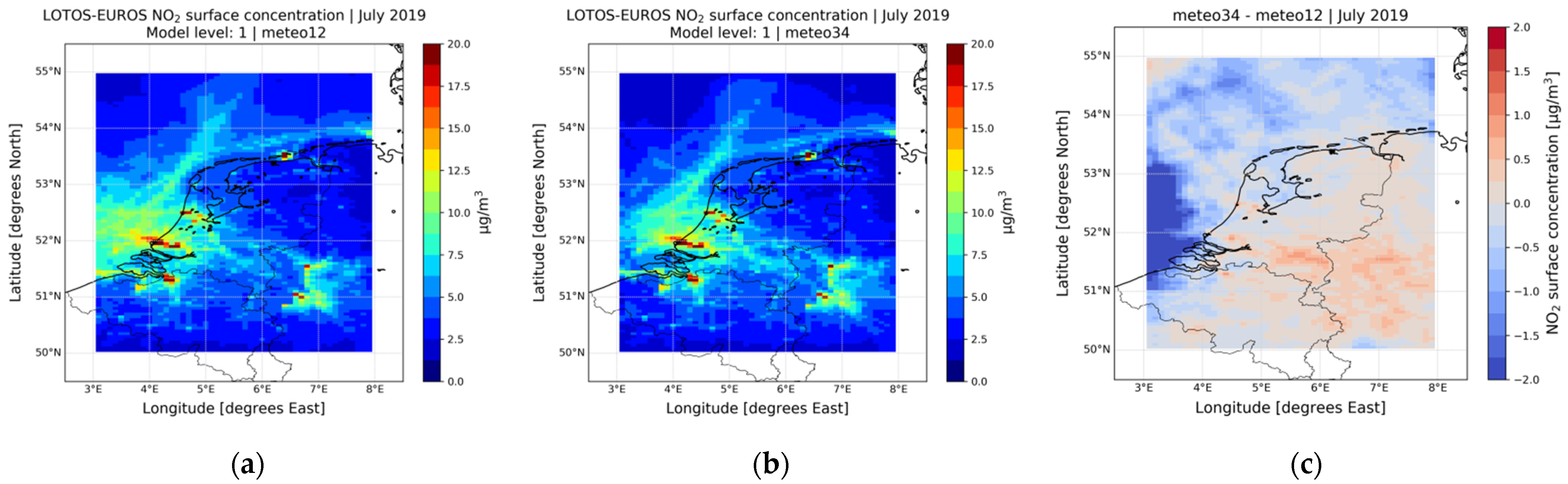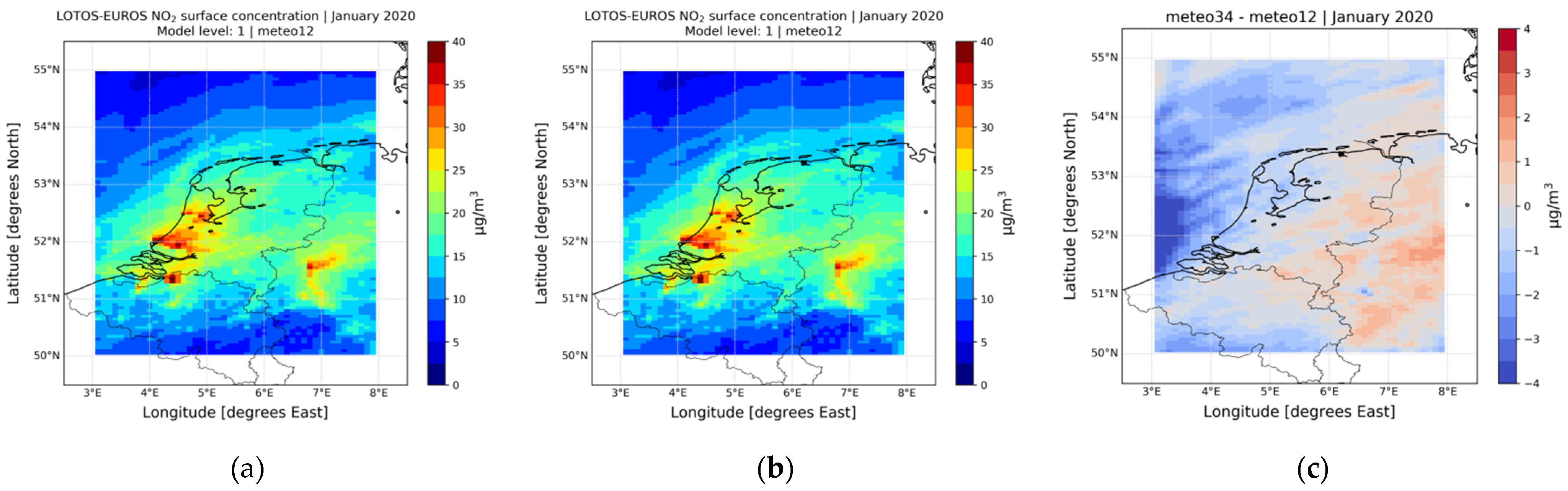Figure 5 shows the LOTOS-EUROS NO₂ surface concentration of the first model layer for both leveling schemes for a zoomed-in area covering the regions of Belgium, western Germany and the Netherlands. At first glance, no significant differences can be spotted between the meteo12 (Figure 5a) and the meteo34 leveling schemes (Figure 5b) NO₂ surface concentrations. By observing the absolute differences between the NO₂ surface concentrations of the meteo34 and the meteo12 schemes (Figure 5c), however, it is evident that the meteo34 leveling scheme results in slightly higher concentrations over high-emitting land areas, by a mean of +1.2 μg/m³, and sharper gradients over hotspots but generally lower concentrations over the sea. The same pattern is also observed in the winter months (Figure A2).

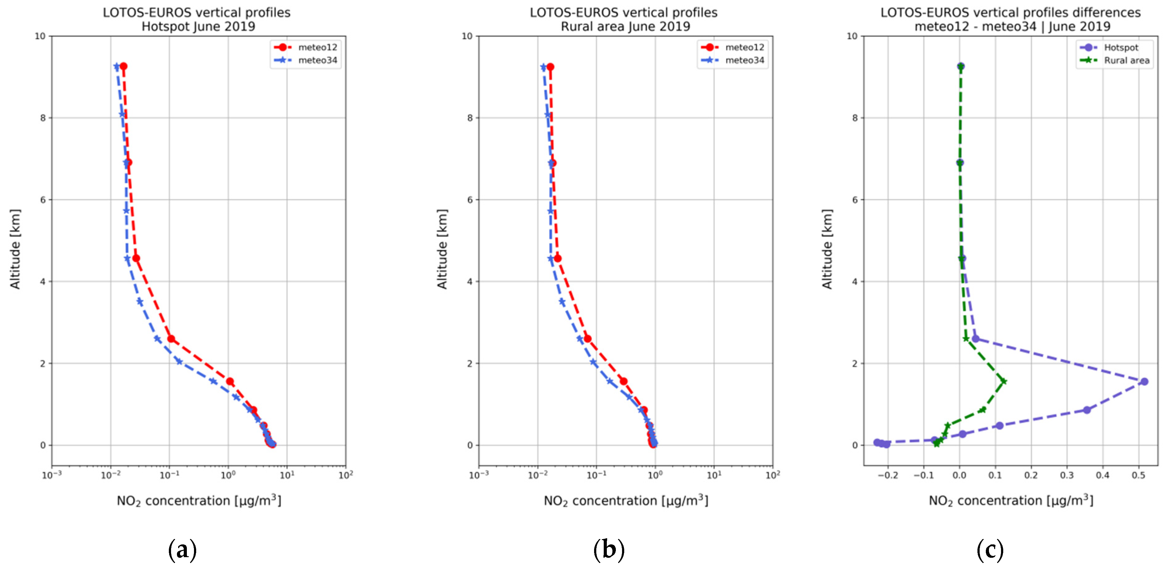
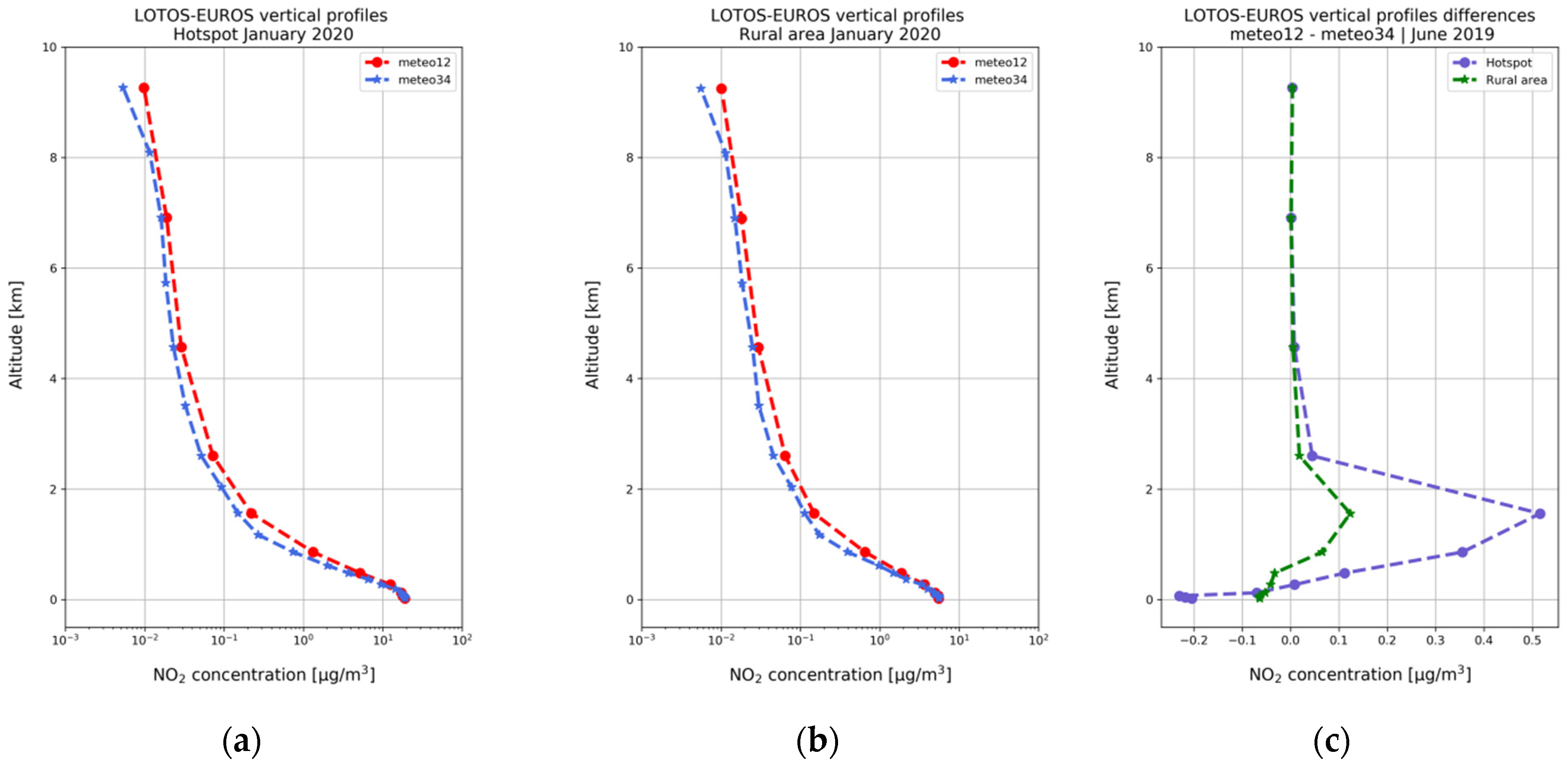
A more detailed view of the differences between the two leveling schemes is shown in the vertical profiles of the modeled NO₂ concentrations (Figure 6) for June 2019 and in Figure A3 for January 2020. Layer interfaces are defined as heights above the surface according to the ECMWF data. Figure 6a and Figure A3a show the vertical profiles of a hotspot pixel while Figure 6b and Figure A3b depict the vertical profiles of a rural pixel. Figure 6c and Figure A3c show the differences between the two vertical schemes. Both hotspot and rural pixels are selected as the closest to a traffic and a rural station in the Netherlands, within the city of Amsterdam. Differences between the vertical profiles of the two leveling schemes are calculated for the first 12 common reference heights, namely the top of each layer from the meteo12 scheme, for both hotspot and rural pixels (Figure 6c and Figure A3c). In both summer and winter, the meteo34 scheme shows higher concentrations for the first three layers. On the contrary, meteo12 shows higher NO₂ concentrations between the fifth and the ninth layer (between 0.12 and 1.5 km), while for higher layers the differences become negligible. Differences are more pronounced for the hotspot pixel, where the meteo34 leveling scheme shows higher NO₂ concentrations for the first three layers by 0.2 μg/m³ in June 2019 and by 0.9 μg/m³ for January 2020 (Figure A3c). The rural differences are an order of magnitude smaller than for hotspot pixels. Overall, for the first model layer, which is used to derive satellite NO₂ surface concentrations, the meteo34 leveling scheme shows 2–4% higher concentrations over the hotspot pixel and 6–10% over the rural pixel for both periods. For the whole central European domain and the first model layer, the meteo34 leveling scheme shows approximately 5% higher NO₂ concentrations for the summer months and 3% for the winter months.

The LOTOS-EUROS NO₂ surface concentrations of the first layer from both leveling schemes are applied to the third setup (Table 1). Inferred TROPOMI v2.3 NO₂ surface concentrations are then estimated for each station type and studied period. The output is two surface products, updated with the new air mass factors and averaging kernels, derived from the two different leveling schemes. Those newly estimated datasets are intercompared for all station types and studied periods in order to assess the effect of the leveling scheme to the implemented methodology.

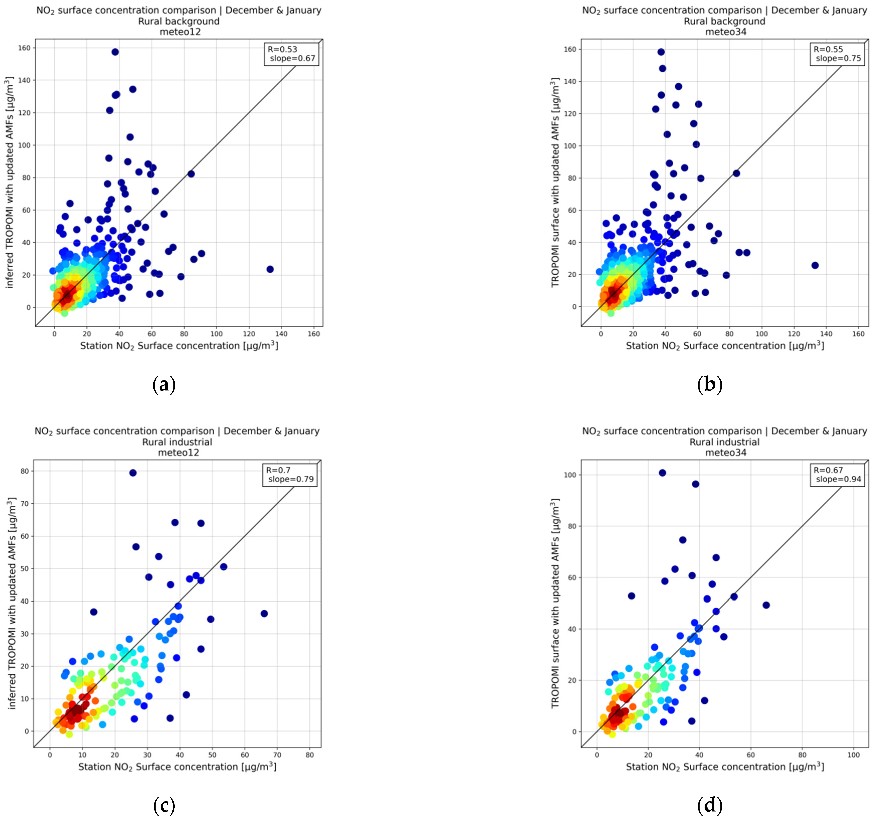
Figure 7 shows the scatter density plots of rural background (Figure 7a) and rural industrial (Figure 7c) stations for the two leveling schemes (Figure 7b,d) for the winter. NO₂ TROPOMI inferred surface concentrations show an overall good agreement with the in situ measurements for both station types with correlation coefficients between 0.53 and 0.7. More specifically, the rural background NO₂ surface concentrations derived from the meteo12 leveling scheme show a correlation of 0.53 and slope of 0.67, whereas the concentrations derived from the meteo34 leveling scheme show a slightly higher correlation (0.55) and a slope of 0.75. Rural industrial correlations are 0.70 and 0.67, and the slopes are 0.79 and 0.94, respectively.

Table 2. Statistics of the comparisons between the inferred and in situ NO₂ surface concentrations for the two leveling schemes in winter.

	Meteo12 Leveling Scheme			Meteo34 Leveling Scheme
Station Type	R	Slope	Relative Bias (%)	R	Slope	Relative Bias (%)
Urban traffic	0.47	0.81	−24.55%	0.48	0.85	−20.70%
Suburban traffic	0.43	0.65	−26.90%	0.45	0.69	−23.18%
Urban background	0.58	1.11	+7.40%	0.58	1.13	+12.00%
Suburban background	0.48	0.78	+3.90%	0.49	0.86	+10.90%
Rural background	0.53	0.67	+10.37%	0.55	0.75	+18.29%
Suburban industrial	0.63	0.76	−15.66%	0.62	0.82	−9.70%
Rural industrial	0.7	0.79	−15.57%	0.67	0.94	−4.32%

and

Table A1. Statistics of the comparison between the inferred and in situ NO₂ surface concentrations for the two leveling schemes and the summer period.

	New Leveling Scheme			Meteo Leveling Scheme
Station Type	R	Slope	Relative Bias (%)	R	Slope	Relative Bias (%)
Urban traffic	0.32	0.13	−77.96%	0.32	0.14	−75.14%
Suburban traffic	0.10	0.03	−78.52%	0.11	0.04	−76.18%
Urban background	0.46	0.38	−45.68%	0.45	0.42	−38.90%
Suburban background	0.52	0.49	−30.58%	0.50	0.54	−21.04%
Rural background	0.46	0.23	−54.31%	0.44	0.24	−47.58%
Suburban industrial	0.58	0.29	−51.54%	0.58	0.32	−46.01%
Rural industrial	0.63	0.34	−37.47%	0.61	0.36	−32.30%

summarize the correlation coefficient, slope, and relative bias of the comparison between the inferred NO₂ TROPOMI v2.3 surface concentrations, derived from each leveling scheme, and the in situ measurements for winter and summer, respectively. Overall, the use of the meteo34 leveling scheme leads to improvements for almost all statistical parameters examined. The urban and suburban traffic stations bias is reduced, from −24.55% to −20.70% and from −26.90% to −23.18%, respectively. Suburban industrial stations bias is lower in the case of the meteo34 leveling scheme (−9.70%) compared to the meteo12 (−15.66%) and the rural industrial stations bias is significantly improved from −15.57% to −4.32%. For background stations, the mean relative bias is slightly higher in the case of the meteo34 leveling scheme for all station types by ~5–7%. Slopes are closer to the 1:1 line for the NO₂ surface concentrations derived from the meteo34 leveling scheme, except for the urban background stations. Correlation coefficients are very similar for both leveling schemes with the highest being calculated for the industrial stations (0.63, 0.62 for the suburban–industrial and 0.7, 0.67 for the rural–industrial stations) and the lowest for the traffic stations (0.47,0.48 for the urban–traffic and 0.43, 0.45 for the suburban–traffic).

In the summer (Table A1), correlations and slopes are generally lower compared to the winter. For traffic stations, correlations range from 0.10 to 0.32 and slopes from 0.03 to 0.14. Relative biases are extremely high for both leveling schemes (~−75%), showing an overall poor agreement with the in situ data. This might be attributed to the higher underestimation of the in situ measurements by the model during the summer. Background stations show better statistical indicators, especially for the NO₂ surface concentrations derived from the meteo34 leveling scheme. Relative biases are lower for the meteo34 leveling scheme by approximately 8% when compared to meteo12. Finally, industrial stations show the highest correlations of all the station types (ranging 0.58–0.63) and the relative bias is lower by ~5% for the surface concentrations derived from the meteo34 leveling scheme.

Overall, the meteo34 leveling scheme yields a better agreement with the in situ measurements. Slopes are closer to 1 and biases are lower for most station types, except for the background stations in winter, where a modest overestimation of the ground-based measurements is found. The only significant drawback of applying the meteo34 leveling scheme to a larger dataset and longer period is that this option is computationally more expensive.

3.1.2. S5P/TROPOMI Versions Comparison

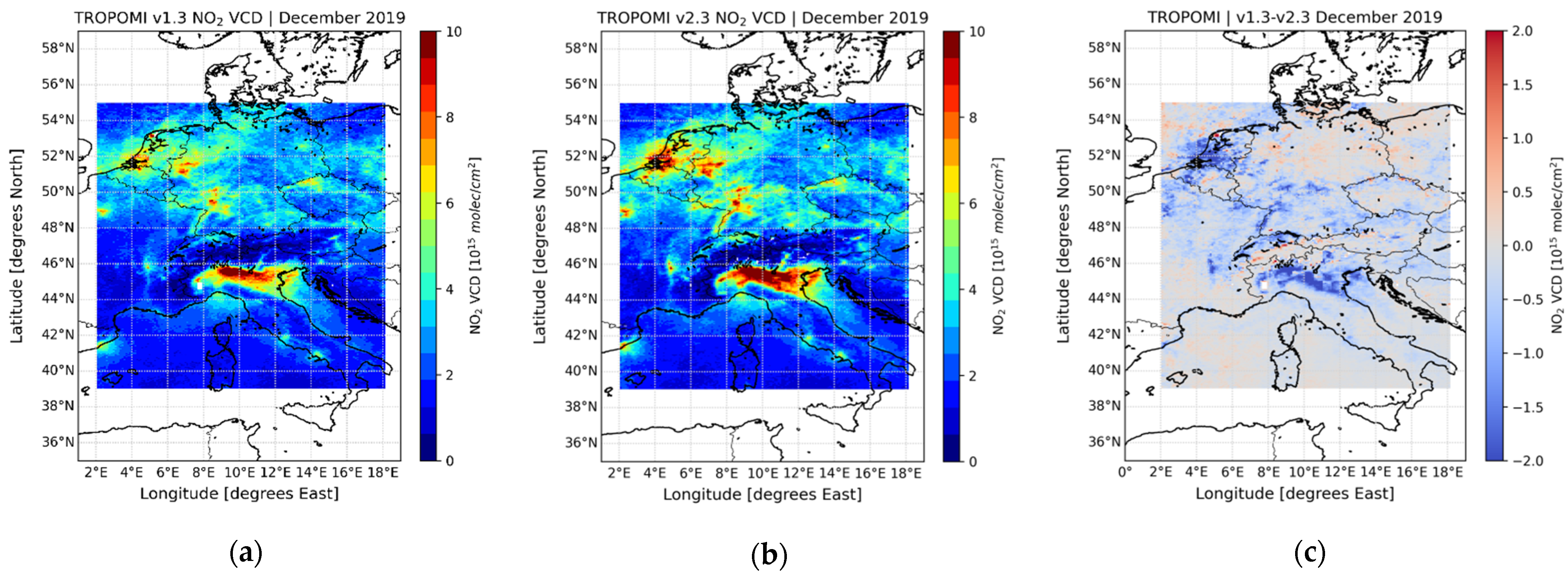
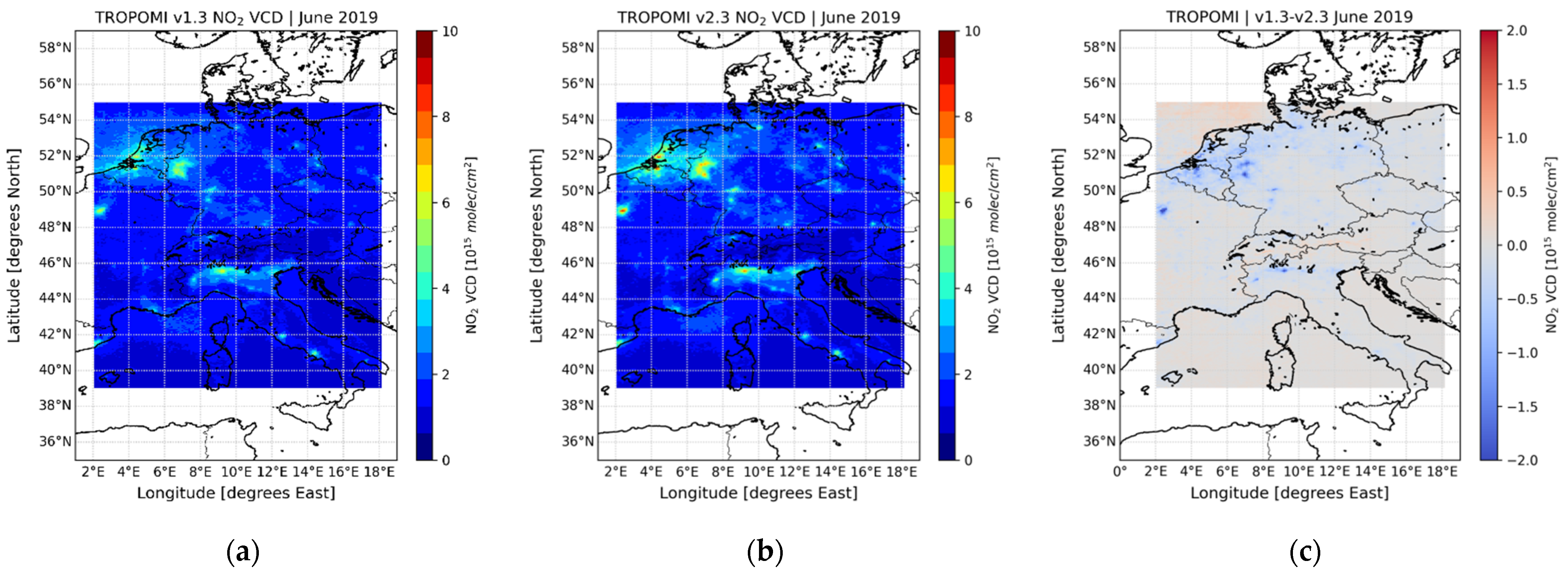
Another quantity that affects the results is the product version of the TROPOMI tropospheric NO₂ VCDs. Figure 1c and Figure A1c have already shown differences between the TROPOMI v1.3 and the TROPOMI v2.3 NO₂ tropospheric VCDs. TROPOMI v2.3 NO₂ concentrations are higher by approximately 3% in summer and by 11–18% in winter. Both v1.3 and v2.3 TROPOMI tropospheric VCDs are used as input in the implemented methodology for all the possible setups (Table 1). Here, the imprint on the derived NO₂ surface concentrations of the third setup is shown for winter. The meteo12 leveling scheme was applied for the LOTOS-EUROS simulations due to computational reasons.

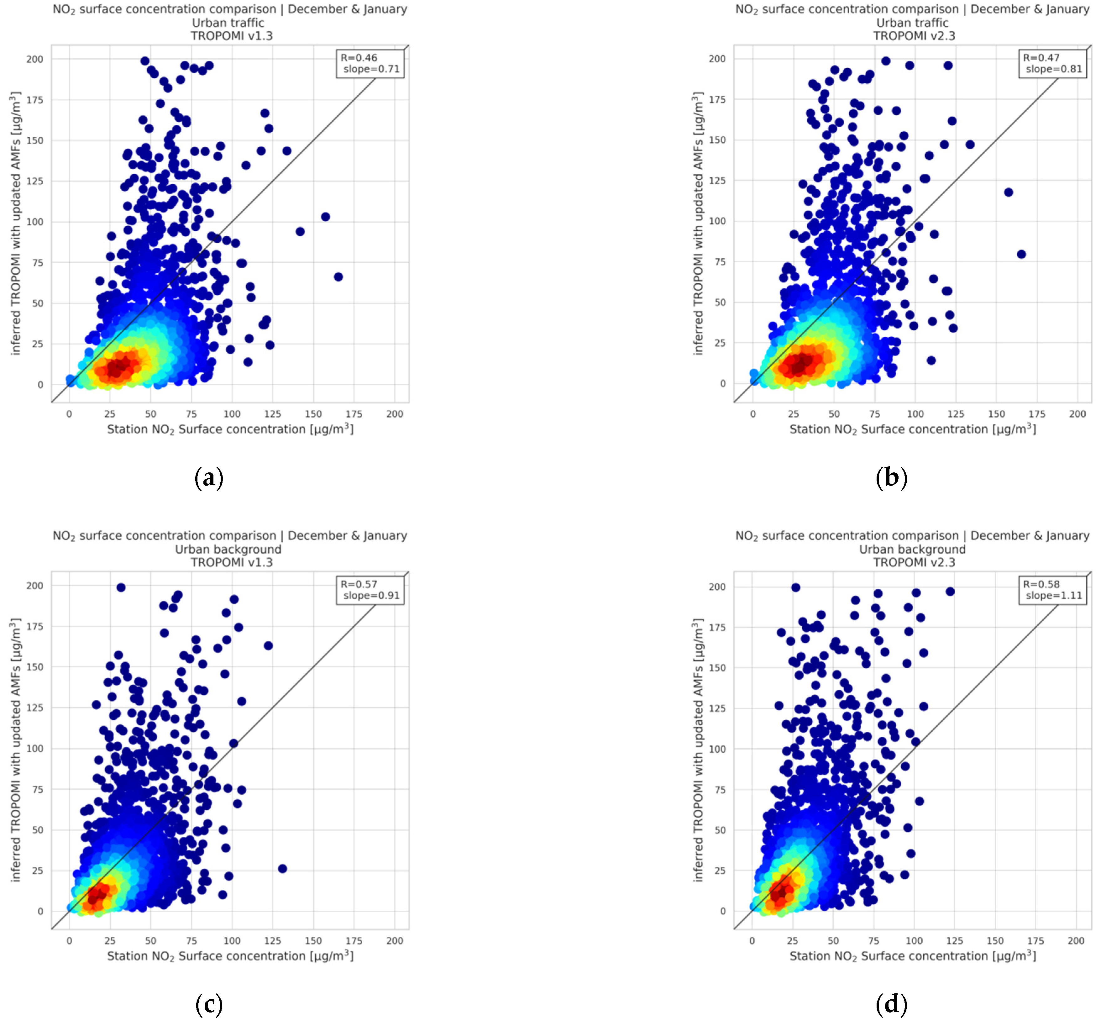
Figure 8 shows the scatter density plots of the urban traffic and background stations between the inferred TROPOMI v1.3 and v2.3 NO₂ surface concentrations of the third setup and the in situ measurements, for the winter. Both versions of TROPOMI inferred NO₂ surface concentrations show nearly identical moderate correlations for both urban traffic and background stations (Figure 8). However, the relative bias is much improved, and the slope is closer to 1 in the case of the TROPOMI v2.3 inferred data, indicating that the concentrations of the latter dataset are closer to the ground-based truth.

The statistical indicators of

Table 3. Statistics of the comparison between TROPOMI v1.3- and v2.3-inferred NO₂ surface concentrations with the in situ measurements for the winter.

	TROPOMI v1.3			TROPOMI v2.3
Station Type	Slope	Absolute Bias *	Relative Bias (%)	Slope	Absolute Bias *	Relative Bias (%)
Urban traffic	0.71	15.46	−35.41%	0.81	10.64	−24.55%
Suburban traffic	0.48	20.19	−44.93%	0.65	11.53	−26.90%
Urban background	0.91	3.86	−12.78%	1.11	−2.21	7.40%
Suburban background	0.73	2.27	−9.94%	0.78	−0.89	3.90%
Rural background	0.66	0.05	−0.25%	0.67	−1.97	10.37%
Suburban industrial	0.56	7.46	−31.79%	0.76	3.77	−15.66%
Rural industrial	0.59	7.55	−38.03%	0.79	3.05	−15.57%

* in μg/m³.

show a significant improvement for the TROPOMI v2.3-derived NO₂ surface concentrations for all station types except from the rural background stations. More specifically, the mean absolute bias of the urban and suburban traffic stations decreases from 15.46 to 10.46 μg/m³ and from 20.19 to 11.53 μg/m³, while there is a significant improvement in the slopes. Urban and suburban background TROPOMI v2.3 NO₂ mean absolute bias improves from 3.86 to −2.21 μg/m³ and from 2.27 to −0.89 μg/m³. Rural background TROPOMI v1.3 NO₂ inferred surface concentrations lay close to the ground-based stations measurements with a mean absolute bias of 0.05 μg/m³, whereas the TROPOMI v2.3 slightly overestimates the in situ measurements with a bias of −1.97 μg/m³. Slopes do not show a major improvement for the TROPOMI v2.3 background-inferred NO₂ surface concentrations. This is possibly related to the known lingering background values issues of the TROPOMI tropospheric NO₂ data [22]. Finally, suburban and rural industrial TROPOMI v1.3 inferred products show a higher bias compared to the TROPOMI v2.3 inferred data, by approximately 15%. Slopes are higher for the industrial TROPOMI v2.3 inferred products, improving from ~0.58 to ~0.78, reinforcing the fact that TROPOMI v2.3 inferred NO₂ surface concentrations correlate better with the in situ measurements. Correlation coefficients are not included in Table 3, as they are shown extensively in Table 2 and are nearly identical for the comparison of both TROPOMI versions. For the summer (

Table A2. Statistics of the comparison between TROPOMI v1.3- and v2.3-inferred NO₂ surface concentrations with the in situ measurements for the summer period.

	TROPOMI v1.3			TROPOMI v2.3
Station Type	Slope	Absolute Bias *	Relative Bias (%)	Slope	Absolute Bias *	Relative Bias (%)
Urban traffic	0.11	29.45	−81.80%	0.81	28.00	−77.74%
Suburban traffic	0.02	25.88	−81.60%	0.65	24.75	−78.52%
Urban background	0.31	7.98	−56.50%	1.11	6.35	−45.61%
Suburban background	0.39	4.82	−43.77%	0.78	3.27	−30.25%
Rural background	0.19	3.47	−59.21%	0.67	3.17	−53.79%
Suburban industrial	0.19	7.76	−64.19%	0.76	6.11	−51.54%
Rural industrial	0.23	4.40	−49.90%	0.79	3.02	−36.62%

* in μg/m³.

), inferred TROPOMI v2.3 NO₂ surface concentrations are slightly higher for all station types by approximately 2 μg/m³. Relative biases are lower by approximately 5%, 14% and 13% for the traffic, background and industrial stations, respectively.

Overall, the comparisons between the TROPOMI versions and the in situ measurements clearly show that the TROPOMI v2.3-inferred NO₂ surface concentrations, after the application of the updated air mass factors, correlate much better with the ground-based measurements.

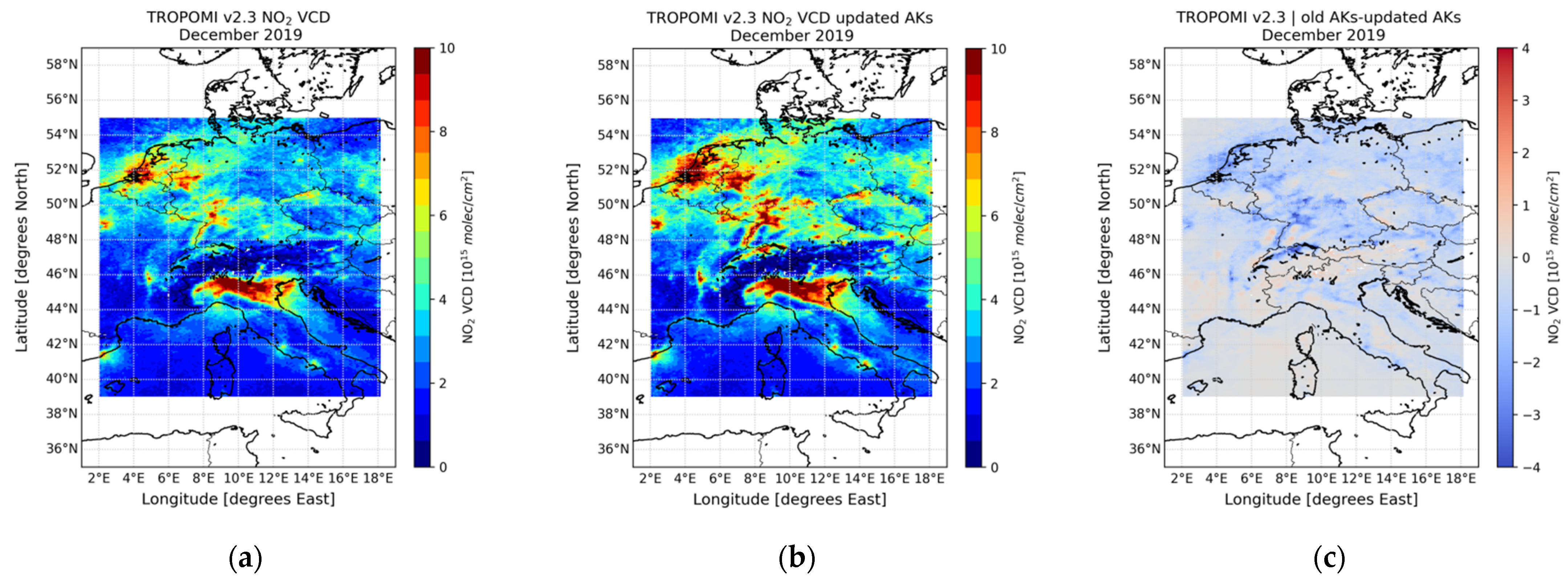
3.1.3. Application of the Updated Air Mass Factors

Another important ingredient in the derivation of NO₂ satellite surface concentrations is the application of the updated air mass factors and averaging kernels to the satellite retrievals (Equation (4)) and the model simulations (Equation (6)) described in the CSO operator process. Therefore, the NO₂ surface products of all possible setups (Table 1) and their comparisons with the in situ measurements are examined in order to determine if the application of the updated air mass factors and averaging kernels improve the results. As concluded in the previous section, TROPOMI v2.3 is optimal for the derivation of satellite NO₂ surface concentrations, and it is therefore used as input in all setups. For the LOTOS-EUROS simulations, the meteo12 leveling scheme was applied to the model configuration, since computational time is important, as the differences between the two leveling schemes are not so important for this analysis.

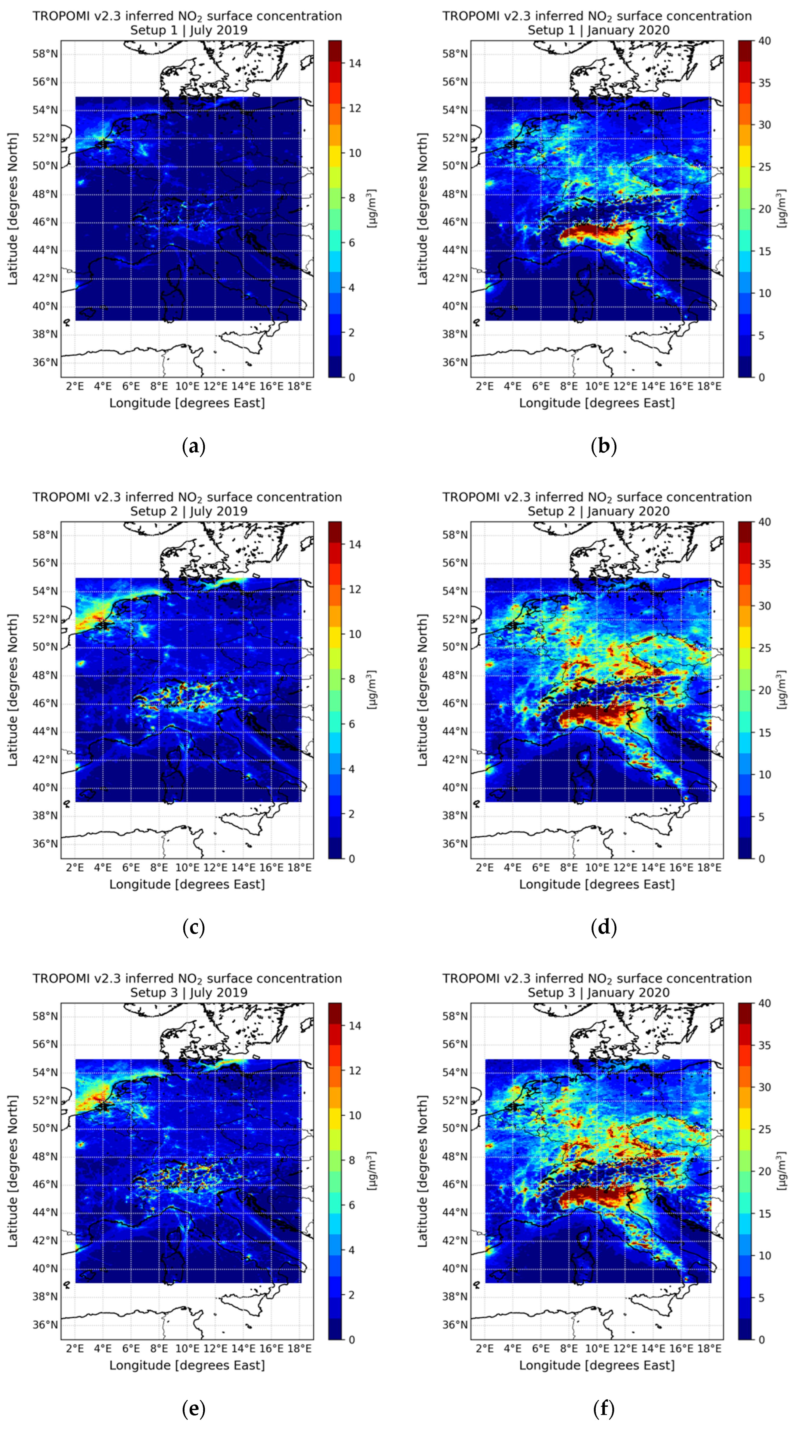
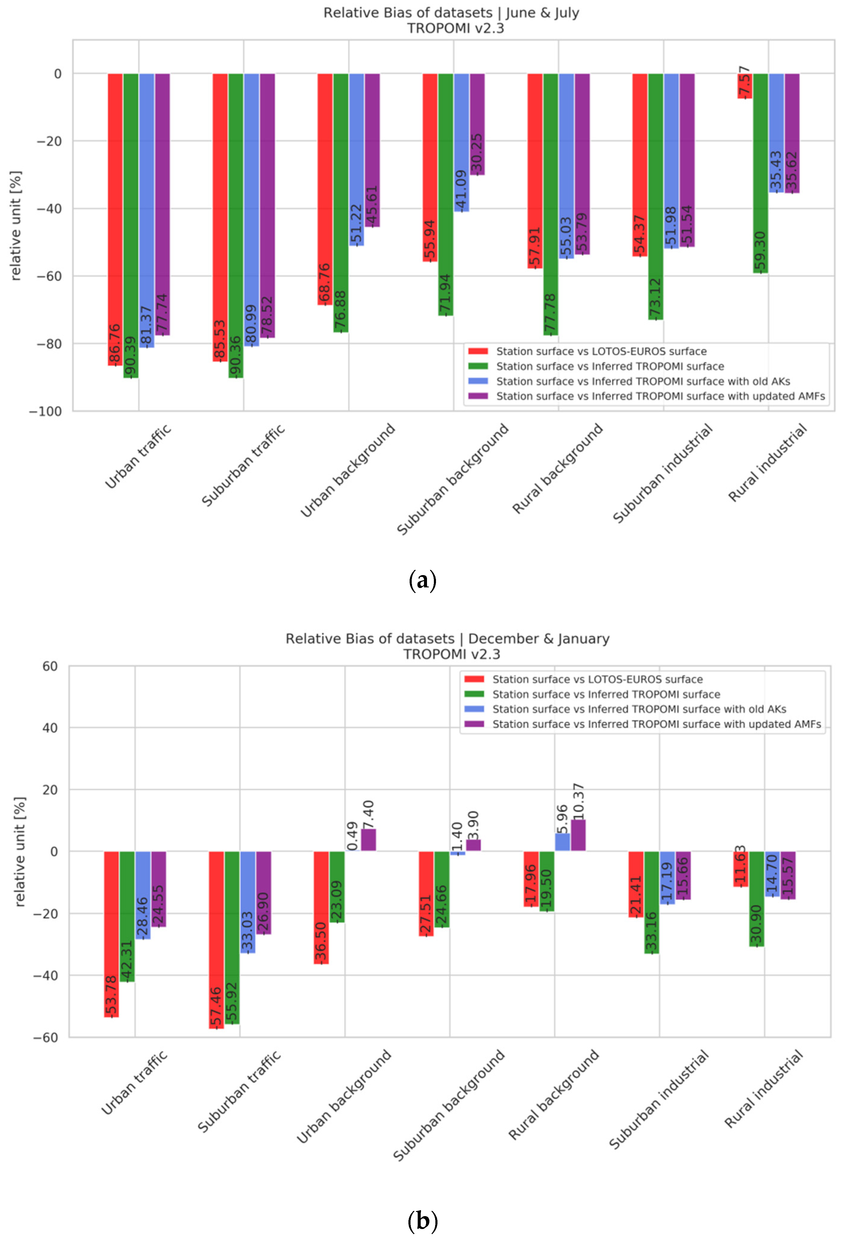
Figure 9 illustrates the relative bias among the inferred TROPOMI NO₂ surface concentrations of all setups and the in situ measurements, and among the LOTOS-EUROS a priori NO₂ surface concentrations and in situ measurements. The relative bias is extremely high for all setups for the urban and the suburban traffic stations, improving from ~−90% in the first setup to ~−78% in the third setup. For all different types of background stations, we find an improved relative bias. Urban background relative bias improves significantly from ~−77% to ~−45% and from ~−72% to ~−30% for the suburban background stations in the third setup. Rural background stations relative bias also decreases for the third setup from ~−78% to −53%, albeit this improvement is not as remarkable as for the urban and suburban background stations. Finally, for the suburban and rural industrial stations the bias notably decreases from ~−73% to ~−51% and from ~−60% to ~−35%, respectively. Worth mentioning is the fact that LOTOS-EUROS relative bias is quite low (~−8%) for the rural industrial stations compared to the other datasets. This can be attributed to the fact that TROPOMI v2.3 NO₂ data seem to underestimate NO₂ levels over the selected rural industrial pixels.

During the winter (Figure 9b), there is an obvious improvement in the relative bias of all the involved parameters with the in situ measurements for all the station types compared to the summer results (Figure 9a). Overall, inferred TROPOMI v2.3 NO₂ surface concentrations derived from the third setup seem to provide a more realistic product, closer to the ground-based truth compared to the baseline setup. More specifically, the bias of the urban and suburban traffic stations shows a remarkable improvement, ~−25% and ~−27%, respectively, by approximately 20–30% when compared to the first setup. Suburban and rural industrial stations bias for the third setup is approximately ~−16%, almost 15% lower for both station types compared to the first setup. For the background stations, a reversal of the sign for the relative bias is evident, considering the absolute levels of NO₂ over the background stations, but still is the lowest compared to the other station types. Inferred TROPOMI v2.3 NO₂ surface concentrations slightly overestimate urban and suburban background in situ measurements by 7.4% and 3.9%, whereas the overestimation is higher (10.37%) for the rural background stations. It is apparent that the second setup (in blue) shows a lower bias for the background stations (0.49%, 1.40% and 5.96%). This can be attributed to the enhancement of the TROPOMI NO₂ tropospheric VCDs by the application of the updated air mass factors and averaging kernels. Finally, inferred TROPOMI NO₂ surface concentrations, derived from the baseline setup, show the highest discrepancies with the in situ measurements for all the station types.

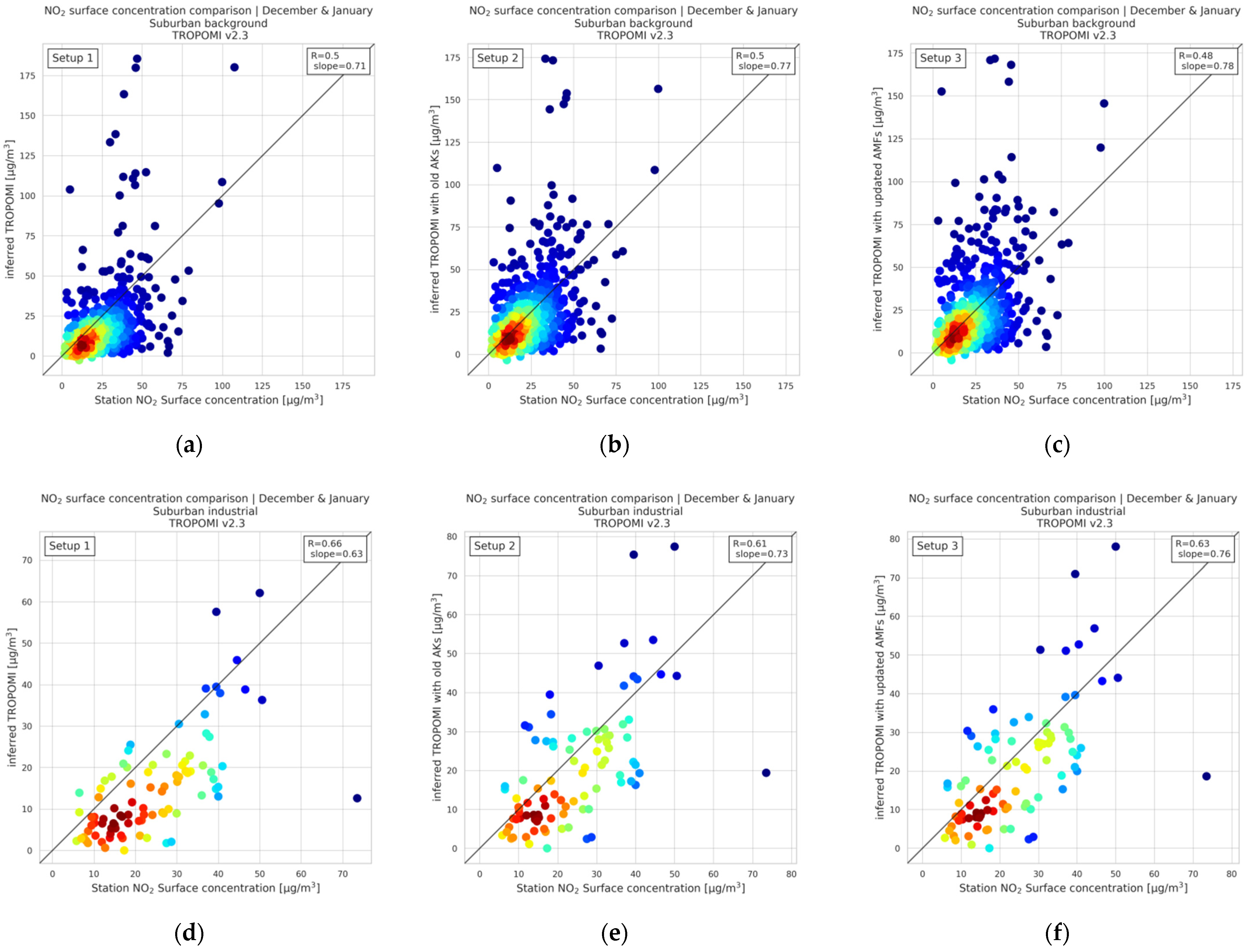
The effect of the air mass factors is better illustrated in the scatter plots of Figure 10. Suburban background (Figure 10a–c) and industrial (Figure 10d–f) stations are depicted. Figure 10a,d, shows the scatter plots between the in situ measurements and the inferred TROPOMI NO₂ surface concentrations of the first setup derived from Equation (7). Figure 10b,e and Figure 10c,f show the same comparisons, including the inferred TROPOMI NO₂ surface concentrations of the second and the third setup, respectively. The TROPOMI-inferred NO₂ surface concentrations of the second setup are calculated with the application of the TM5-MP averaging kernels to the LOTOS-EUROS simulations, whereas the inferred NO₂ surface concentrations of the third setup are estimated with the application of the updated air mass factors and averaging kernels on both the TROPOMI data and the model simulations. An improvement of the slope is found for both the second and third setup, from 0.71 to 0.77 and 0.78 and from 0.63 to 0.73 and 0.76, respectively. This statistical indicator shows that the third setup performs better compared to the other two setups, and the derived NO₂ surface concentrations are closer to the ground-based data. Correlation coefficients are moderate for the suburban background station (R~0.5) and good for the suburban industrial stations (R~0.65), varying insignificantly for each setup.

Concluding, it is obvious that the TROPOMI-inferred NO₂ surface concentrations of the third setup perform better overall. Biases are significantly lower insummer. In winter, there is a remarkable improvement for the traffic and industrial stations; whereas, for the background stations, a slight overestimation is found, which, however, does not exceed the threshold of 10%. We should underline the fact that the second setup performs better for the background stations.

3.2. Optimal Setup

We have already shown the effect of the three prominent influencing quantities on the satellite-derived NO₂ surface concentrations. The application of the meteo34 leveling scheme on the model simulations generates higher inferred TROPOMI NO₂ surface concentrations over land, resulting in a lower bias for all the station types during both periods, except from the background stations during the winter months. Although the results are generally improved, we proceeded using the meteo12 leveling scheme mainly due the high computational time required for the meteo34 leveling scheme simulations. TROPOMI v2.3 NO₂ tropospheric VCDs perform better, and the performance is further enhanced with the application of the updated air mass factors on both the TROPOMI data and the model simulations. Hence, the optimal setup comprises the TROPOMI v2.3 NO₂ VCDs, the meteo12 leveling scheme LOTOS-EUROS simulations and the updated air mass factors and averaging kernels applied on the satellite data and the LOTOS-EUROS simulations (setup 3 in Table 1).

The simplified Lamsal equation (Equation (7)) introduced significant capabilities in the derivation of satellite NO₂ surface concentrations. However, the simple application of the a priori model simulations and original satellite data in Equation (7) produces poor results when compared to ground-based data, as shown in Figure 11. Overall, the NO₂ surface concentrations derived from the optimal setup offer a better match with the ground-based measurements for both periods. During summer, background and industrial stations exhibit the lowest bias. The differences with the in situ measurements range between 3 and 6 μg/m³ and are lower by 2–4 μg/m³ when compared to the differences in the baseline setup with the ground-based data. Traffic urban and suburban stations show a high mean absolute bias of 28 and 25 μg/m³ with the in situ measurements, but this is still much improved compared to the derived NO₂ surface concentrations from the baseline setup.

During winter, the inferred NO₂ surface concentrations of the optimal setup lie close to the ground-based concentrations of the background stations, with the lowest biases calculated for urban, suburban and rural areas, −2.22, −0.89 and −1.97 μg/m³, respectively. This can be attributed to the high known NO₂ loads observed by TROPOMI over background areas [23] and the enhancement of NO₂ levels due to the application of the updated air mass factors and averaging kernels. Industrial station differences are 3–4 μg/m³_, almost 50% lower than the baseline setup. Finally, traffic stations bias shows major improvement with a mean value ~11 μg/m³, notably lower by ~8–10 μg/m³ than the baseline setup. Note that the TROPOMI and LOTOS-EUROS resolution is, unavoidably, too low to properly resolve the high concentrations at traffic stations, resulting in higher biases. However, the implementation of the local air mass factors to the satellite NO₂ VCDs and the model simulations do reduce the bias at the traffic stations. Summarizing the aforementioned findings,

Table 4. In situ and TROPOMI v2.3-inferred mean NO₂ surface concentrations and standard deviations (in μg/m³) for the first and third setups and both periods.

	Summer			Winter
Station Type	In Situ	Setup 1	Setup 3	In Situ	Setup 1	Setup 3
Urban traffic	36.02 ± 6.00	3.46 ± 1.86	8.02 ± 2.83	43.34 ± 6.58	25.00 ± 5.00	32.70 ± 5.72
Suburban traffic	31.52 ± 5.61	3.04 ± 1.74	6.77 ± 2.60	42.87 ± 6.55	18.90 ± 4.35	31.34 ± 5.60
Urban background	13.92 ± 3.73	3.21 ± 1.79	7.57 ± 2.75	29.30 ± 5.48	23.06 ± 4.80	32.20 ± 5.67
Suburban background	10.81 ± 3.29	3.03 ± 1.74	7.54 ± 2.75	22.85 ± 4.78	17.21 ± 4.15	23.73 ± 4.87
Rural background	5.90 ± 2.43	1.31 ± 1.15	2.73 ± 1.65	18.96 ± 4.35	15.27 ± 3.91	20.93 ± 4.87
Suburban industrial	11.86 ± 3.44	3.19 ± 1.79	5.75 ± 2.40	24.06 ± 4.91	16.08 ± 4.01	20.29 ± 4.58
Rural industrial	8.49 ± 2.91	3.45 ± 1.86	5.47 ± 2.34	19.59 ± 4.43	13.53 ± 3.68	16.54 ± 4.07

shows analytically the mean NO₂ surface concentrations of the EEA stations for the baseline and the optimal setup for both periods.

It is clear that the ad hoc implementation of the described baseline methodology with the original satellite and model data results in significant discrepancies with the ground-based truth. The product improves significantly when accounting for the effect of the new TROPOMI product version, averaging kernels and air mass factors. Thus, the derivation of NO₂ surface concentrations is a complicated problem that requires sufficient knowledge on the existing methodologies and quantities that can bring the results closer to the ground truth.

4. Conclusions

The aim of this study is to derive NO₂ surface concentrations over Central Europe from the S5P/TROPOMI instrument. To achieve this objective, we implemented the methodology originally described by the work of [9], for three different setups. The first setup, which is the baseline setup, includes the a priori TROPOMI v1.3 and v2.3 tropospheric NO₂ VCDs and the a priori LOTOS-EUROS simulations of NO₂ VCDs and surface concentrations. The second setup includes the a priori TROPOMI NO₂ VCDs and the LOTOS-EUROS simulations, in which the averaging kernels of the TM5-MP model have been applied. Finally, the third setup includes the modified TROPOMI and LOTOS-EUROS NO₂ tropospheric VCDs after the application of the updated air mass factors and averaging kernels via the CSO process and the a priori LOTOS-EUROS NO₂ surface concentrations. The derived concentrations from all setups are compared with EEA in situ measurements. Furthermore, three important influencing quantities that directly affect the results, namely the LOTOS-EUROS leveling scheme, the TROPOMI NO₂ product versions and the updated air mass factors and averaging kernels, were examined thoroughly. The main findings of the study are summarized below.

• The LOTOS-EUROS meteo34 vertical leveling scheme showed overall improved statistical indicators. Slopes are closer to 1, and the relative bias is lower. In particular, the relative bias in summer is lower for traffic stations by approximately 2%, for background stations by 7–9% and for the industrial stations by 5% compared to the relative bias of the meteo12 scheme. During winter, traffic and industrial stations relative bias is lower by 4–11%. Meteo34 background stations inferred NO₂ TROPOMI v2.3 surface concentrations are higher by 5–7% compared to the meteo12. Overall, the meteo34 leveling scheme performs better, but it is computationally more expensive. Thus, the meteo12 leveling scheme was implemented in the further experiments.
• TROPOMI v2.3-inferred NO₂ surface concentrations showed overall better agreement with the ground-based measurements. The relative bias is lower by ~10% and ~18% for the traffic urban and suburban stations compared to the TROPOMI v1.3 -derived surface datasets. Urban and suburban background stations show a slightly lower bias of 5–6%, whereas the rural background stations bias is higher (~10%) than the TROPOMI v1.3 bias (~−0.25%). Finally, suburban- and rural- industrial-inferred TROPOMI v2.3 NO₂ surface concentrations show an improved relative bias with the ground-based data (from ~−35% to ~15%).
• The derived TROPOMI v2.3 NO₂ surface concentrations, updated with the air mass factors and averaging kernels from the local model (third setup), lie closer to the ground-based truth for both periods. In summer, biases are high for the traffic stations (~−70%) and moderate for background and industrial stations, ranging from −50% to −30%, improving significantly compared to the first setup. In winter, traffic and industrial stations bias improves from −50% to −25% and from −30% to −15%. Background-station-inferred NO₂ surface concentrations slightly overestimate the ground-based measurements in winter. In this case, the second setup shows a lower bias for the urban (+0.49%), suburban (+1.40%) and rural (+5.96%) background stations compared to the third setup (+7.40%, +3.90% and +10.37%, respectively). This enhancement can be attributed to the sharper gradients included in the updated air mass factors. Comparisons between the first and the third setups show an average improvement of 24% and 18% in the bias of summer and winter, respectively.
• The implemented methodology performs better for the background and industrial stations for both periods. This may be attributed to the fact that TROPOMI and LOTOS-EUROS resolution is too low to properly resolve the high concentrations at traffic stations, resulting in higher net biases.
• Results are better in winter for all station types. Model simulations are obtained only at 11:00 UTC, which is the closest time to the TROPOMI overpass. The model underestimates the in situ NO₂ surface concentrations during daytime and the underestimation is higher in summer. This might be attributed to the higher photolysis rate of NO₂ in summer (higher solar radiation, low cloud cover), which is maximized in the early afternoon. Summer NO₂ levels are significantly lower and closer to the emission sources compared to the winter, when the NO_X lifetime is higher and local transport of emissions is more pronounced. Low resolution (0.10° × 0.05°) model simulations and satellite observations cannot detect emissions at station level, especially in summer, due to representation issues related to the location of the stations. Differences between both periods might also be partly attributed to the anthropogenic NO_X emissions used in the model, as they refer to year 2017.

Overall, the derived TROPOMI v2.3 NO₂ surface concentrations of the third setup show the best agreement with the in situ measurements. The ultimate goal of this study is to provide inferred S5P/TROPOMI NO₂ surface concentrations with a reliable methodology, for areas where in situ measurements are not available. The third setup, which is optimal, seems to respond sufficiently to this task with room for improvement.