Article

Hydrological Drivers for the Spatial Distribution of Wetland Herbaceous Communities in Poyang Lake

1
College of Water Conservancy and Hydropower Engineering, Hohai University, Nanjing 210098, China
2
Nanjing Hydraulic Research Institute, Nanjing 210029, China
3
Institute of Bio- and Geosciences: Agrosphere (IBG-3), Forschungszentrum Jülich, 52428 Jülich, Germany
4
School of Natural Sciences, Environment Centre Wales, Bangor University, Bangor LL57 2UW, UK
5
Jiangxi Poyang Lake Nanji Wetland National Nature Reserve Authority, Nanchang 330038, China
6
School of Agriculture and Horticulture, Chengdu Agricultural College, Chengdu 611130, China
*
Author to whom correspondence should be addressed.
Remote Sens. 2022, 14(19), 4870; https://doi.org/10.3390/rs14194870
Submission received: 29 August 2022 / Revised: 27 September 2022 / Accepted: 28 September 2022 / Published: 29 September 2022
(This article belongs to the Special Issue Remote Sensing of Wetlands and Biodiversity)

Abstract

:
Hydrological processes are known as major driving forces in structuring wetland plant communities, but the specific relationships are not always well understood. The recent dry conditions of Poyang Lake (i.e., the largest freshwater lake in China) are having a profound impact on its wetland vegetation, leading to the degradation of the entire wetland ecosystem. We developed an integrated framework to quantitatively investigate the relationship between the spatial distribution of major wetland herbaceous communities and the hydrological regimes of Poyang Lake. First, the wetland herbaceous community classification was built using a support-vector machine and simultaneous parameter optimization, achieving an overall accuracy of over 98%. Secondly, based on the inundation conditions since 2000, four hydrological drivers of the spatial distribution of these communities were evaluated by canonical correspondence analysis. Finally, the hydrological niches of the communities were quantified by Gaussian regression and quantile methods. The results show that there were significant interspecific differences in terms of the hydrological niche. For example, Carex cinerascens Ass was the most adaptable to inundation, while Triarrhena lutarioriparia + Phragmites australis Ass was the least. Our integrated analytical framework can contribute to hydrological management to better maintain the wetland plant community structure in the Poyang Lake area.

Graphical Abstract

1. Introduction

The water level is essential in determining wetland plants’ ecological characteristics, biomass accumulation, and reproductive patterns [1,2]. Fluctuations in wetland water levels impact plant colonization and expansion, primary productivity, community composition, species diversity, and community succession, and they play an essential role in wetlands’ development, maintenance, and extinction [3]. There are many similar lakes around the world that face the problem of fluctuating wetland water levels affecting plant communities. For example, droughts affect the coastal wetland of Lake Huron, with larger impacts on the vegetation [4]. Similarly, the vegetation distribution and the structuring of wetland environments in the Everglades National Park, near the Gulf of Mexico, is also modified by hydrological dynamics caused by human interaction and climate change [5]. As a dynamic wetland system, Poyang Lake in China provides critical ecological functions for water circulation and biodiversity conservation. It is known for its dynamics between floods and low water levels, creating a unique landscape where high water levels exhibit a lake and low water levels exhibit a river [6]. Large areas of lakeshores are exposed during the dry season, providing favorable conditions for the growth of wetland vegetation communities. This wetland ecosystem, composed of grass flats, mudflats, and waterbodies, provides habitats and foraging places for fish and winter migratory birds [7]. Unfortunately, the low water levels and dry periods are prolonged in Poyang Lake due to intensive human activities (e.g., discharge regulation at the Three Gorges Dam, sand dredging, water use for agriculture) and changing climate, which have led to a significant alteration in the dominant species of the wetland vegetation community [8,9,10,11]. Studies have shown that the continuously low water level of the Poyang Lake in recent years (especially after 2000) has caused a downward shift in the elevation of vegetated areas [8,9,12]. As a result, the aquatic vegetation has been declining, and a large area of mudflats has been invaded by terrestrial vegetation [9,11,13].
The various vegetation communities are critical for wintering waterbirds to choose a well-suited foraging and nesting environment [7,14,15]. Poyang Lake’s wetland vegetation is dominated by grass and aquatic vegetation, composed of various wet plants, marsh plants, and aquatic plants [16]. Affected by many factors (such as lake microtopography, water regime, groundwater depth, soil structure, and other factors)—especially the water level changes—the distribution of vegetation along the inundation gradient shows a community mosaic and a community complex structure [17]. For example, in meadows, the communities often appear in patches [18]. Therefore, it is challenging for researchers to map a detailed vegetation community distribution. Fortunately, remote sensing techniques can provide a cost-effective means of monitoring and capturing empirical relationships between in situ data and satellite data [19,20,21]. Although remote sensing provides efficient tools for wetland mapping and monitoring, there are various technical limitations in wetland classification [20,22]. For instance, conventional supervised classifiers might be inefficient for identifying wetland plant communities [23,24]. Moreover, wetland plant communities with similar spectral and backscattering behavior in optical and synthetic aperture radar (SAR) data may confuse classification [24]. Additionally, advanced techniques such as high-resolution satellite images and near-ground remote sensing are widely used in plant community ecology studies at different scales, and the results indicate that high spatial resolution aids in mapping those heterogeneous wetlands at the scale of herbaceous plant communities [25,26,27]. However, most studies are based on coarse-resolution data (i.e., more than 10 m × 10 m) to encompass such a diverse vegetation community in the dynamic wetlands [13,28,29]. In this case, multiple vegetation community groups can be found in one pixel [5]. Hence, delineating the precise boundary of each vegetation community surrounding the point using fine-spatial-resolution imagery is challenging.
On the other hand, collecting reference samples is a prerequisite for accurately supervised classifications. Insufficient and unrepresentative reference samples have been recognized as the primary sources of error in the supervised classifications [30,31,32]. Many studies have found that wetland classifications benefit from dense field data—particularly wetland mapping [33,34]. However, input variable selection is critical in developing supervised classification models, which should be relevant and non-redundant to avoid adding noise to the models and increasing model complexity [35]. On the other hand, omitting relevant input variables can make the models less accurate and unable to fully describe the system behavior [36]. Therefore, input variables are essential for the model’s computation time and classification accuracy in classifying complex wetland herbaceous communities.
Hydrological regimes create niches for colonizing different types of vegetation [37]. The dynamic relationship between the hydrological regime and the vegetation can be complex, experiencing periodic flooding that exhibits changes in the spatial distribution and temporal duration of inundation areas [38,39]. Due to differences in water demands/tolerances between species and the competitive interactions of different communities, changes in hydrological conditions may alter the dominance of species [40,41]. The impacts are most pronounced in shallow water, where even small fluctuations in lake levels can cause the environment to switch from one of standing water to one where sediments are exposed to the air, or vice versa [41]. As a result, they can boost flooding-related mortality or plant seed bank germination. Hence, hydrological factors such as water level, water depth, and inundation duration are regarded as key factors for the distribution of wetland herbaceous communities [5,42]. The impacts of variable hydrological processes on vegetation distribution have been investigated previously in the Poyang Lake wetland using linear regression and sensitivity index [28,29,43]. These results reveal the response patterns and change trends of wetland plants in Poyang Lake in response to hydrological processes from different perspectives and scales. In contrast, relatively few studies have analyzed and quantified wetland vegetation’s water demand from the perspective of ecological niche [44,45,46]. Moreover, traditional studies of vegetative hydrological niches focus more on the mechanistic and microscopic levels [47]. More detailed analysis with sufficient in situ data and classification at smaller scales is required to address vegetation distribution patterns in complex and variable wetland water environments. Therefore, a better understanding of how the hydrological system affects wetland herbaceous communities’ distribution is crucial for monitoring and habitat assessment of wetland ecosystems.
Given this background, the main purpose of this study was to develop an integrated framework to quantify the spatial distribution of the dominant vegetation communities in response to inundation, and to propose criteria for discriminating the spatial distribution of these communities. Specifically, this study aimed to (i) develop a wetland herbaceous community classification model based on machine learning to map the detailed communities; (ii) analyze the hydrological regime’s influence mechanisms on the spatial distribution of the wetland herbaceous communities based on the changes in the historical water level dynamics since 2000; and (iii) quantify the hydrological niches of the dominant vegetation communities. This study is expected to improve the understanding of the hydrological effects on vegetation communities in the Poyang Lake wetland.

2. Materials and Methods

2.1. Poyang Lake and Nanji Wetland National Nature Reserve

Poyang Lake (28°11′–29°51′N, 115°31′–117°06′E) is located in the southern bank of the lower reaches of the Yangtze River Basin (Figure 1a), with a catchment area of about 162,000 km2. This area belongs to the subtropical zone, with a mean annual precipitation of 1400–2400 mm and a mean annual air temperature of 16–19 °C [48]. It receives catchment inflows from five major tributaries (Xiushui River, Ganjiang River, Fuhe River, Xinjiang River, and Raohe River) and discharges to the Yangtze River at Hukou in the north (Figure 1a). Due to the heterogeneity of precipitation and the connectivity of the rivers to Poyang Lake, the lake area fluctuates wildly throughout the year. The lake area is 735, 2670, and 3190 km2 at water levels of 10, 14, and 19 m (Xingzi Station), respectively [49]. Formed by a combination of lacustrine rivers, the lake has a complex topography, including narrow channels, periodically separated lakes, and large areas of seasonally inundated alluvial deltas [50]. Under the combined effects of natural and human activities, 102 dish-shaped lakes were formed in the estuarine delta formed in the Poyang Lake [51].
There are two national nature reserves in Poyang Lake. The largest is the Nanji Wetland National Nature Reserve (NWNNR), listed as an internationally important wetland by the Ramsar Convention. It is located in the southern region of Poyang Lake (Figure 1b), covering an area of 333 km2. The NWNNR was classified into a sub-lake zone and a wetland zone in terms of the hydrological and geographic settings [52]. The study area on Dong Lake’s shore belongs to the wetland zone and covers 1.29% of the NWNNR (Figure 1c). As a part of the Poyang Lake floodplain, this reserve experiences considerable seasonal water level fluctuations [53].
Subtropical monsoons in Poyang Lake lead to strong seasonality in precipitation, resulting in complex topography and dramatic variations in the total water coverage within a year [12]. Annual average fluctuations in water levels (Xingzi Station) vary by 8~18 m [54]. From April to September (i.e., the wet season), almost all sub-lakes of the Poyang Lake are connected to form a large lake, with an area peaking at approximately 4000 km2 [13,29]. This period is also a growing season for aquatic vegetation and high-elevation grasses [26]. From October to March (i.e., the dry season), the lake is divided into many segments separated by the exposed floodplains, becoming a complex assembly of distinct hydrological rivers and shallow waters interspersed with meadows, with a small inundation area of less than 1000 km2 [9]. At this time, the exposed lake mudflats are gradually colonized by emergent vegetation during the growing season [26,55,56].
The alternating land–water transition zone (i.e., fluctuation zone) between the wetland’s highest and lowest flood levels essentially delineates the range of vegetation types in the wetland. Under seasonal flood inundation stress, the vegetation in the wetland shows a regular spatial distribution pattern along the elevation. Reeds, sedges, and aquatics are distributed from the high region to the low region [9]. The dominant wetland herbaceous communities in the study area are Triarrhena lutarioriparia + Phragmites australis Ass (Triarrhena Ass), Carex cinerascens Ass (Carex Ass), and Phalaris arundinacea Ass (Phalaris Ass) [8,57] (Table 1). Under severe summer flood conditions, high mortality rates occur in herbaceous communities [49]. During the fall months, the Carex Ass initiates regrowth as the soil is exposed, and the Triarrhena Ass enters the booting and heading stage, while Phalaris Ass withers gradually [9,29].
The spatial variability of hydrological and wetland vegetation dynamics provides heterogeneous habitats and abundant food for migratory waterbirds in the form of stopovers and wintering places [61]. The NWNNR is the key node on the East Asia–Australia waterfowl migration route for migratory waterbirds, some of which are listed as nationally protected wildlife species in China (e.g., the Oriental stork (Ciconia Boyciana), the hooded crane (Grus Monacha), and the Siberian crane (Grus leucogeranus)) [7,62].

2.2. Data Acquisition

2.2.1. Field Sampling Data

The period with high vegetation cover of Poyang Lake is the dry season, and physical access to many wetlands is hindered by the water being too shallow for direct access. Comprehensive field studies have focused on the Dong Lake transection in the NWNNR, balancing admittance, accessibility, and the acquisition of a representative sample of the NWNNR (Figure 1c). To improve vegetation survey efficiency to obtain ground reference data over large areas, the surveys during the winter of 2020 were carried out as follows: An unmanned aerial vehicle (UAV, DJI Phantom 4) survey provided aerial high-resolution RGB imagery. A spatial true-color map was developed based on this imagery using Pix4D software, which was used to delineate the corresponding boundary of each vegetation community (Figure 1c). Finally, we checked and sampled the field to determine the complex and ambiguous areas of plant community distribution.
At georeferenced locations of a 10 m × 10 m (i.e., one pixel of Sentinel-2) grid, we recorded which plant community dominated (i.e., covered more than 50%). A total of 42,590 such grid cells were recorded during these surveys to obtain training and validation data. Seven classes were distinguished: (1) Triarrhena Ass, (2) Carex Ass, (3) Phalaris Ass, (4) mudflats (with some Carex cinerascens Ass), (5) sand, (6) water, and (7) mixed pixels (i.e., pixels that could not be defined as dominated by one community).

2.2.2. Remote Sensing Data

A cloud-free Sentinel-2A Multispectral Instrument (MSI) scene (Sentinel Scene Identifier: S2A_MSIL1C_20201222T025131_N0209_R132_T50RMT_20201222T051459) was acquired from the ESA Sentinels Scientific Data Hub on 22 December 2020 (the same date when the field sampling took place). Its processing level 1C includes radiometric and geometric corrections with sub-pixel accuracy [63]. On this basis, the atmospheric correction was performed using the Sen2cor plug-in in the Sentinel Application Platform (SNAP) software provided by the ESA to facilitate subsequent band calculations. With this step, the widely used L2C was achieved [64,65]. We refrained from conducting a topographic correction because the study area is a floodplain [26]. The MSI instruments of Sentinel-2 have three spatial resolutions (i.e., 10, 20, and 60 m). All coarser bands were then resampled to 10 m by nearest-neighbor resampling to match the higher-resolution bands. We further calculated each pixel’s most common multispectral indices (e.g., NDVI, EVI, and RVI; more details in Table A1) as a database for the classification model.

2.2.3. Hydrological and Topographic Data

The daily lake stages at the nearest gauging station of the study area (i.e., at Kangshan; Figure 1b) from 2000 to 2020 were used to reflect the inundation dynamics of the study area. The digital elevation model (DEM) was obtained from Jiangxi Province, and was used in conjunction with the measured water level to calculate the water depth of each pixel. The DEM elevation and water level elevation references were consistent.

2.3. Methodology

For this study, a framework was designed to quantitatively investigate the spatial distribution of the dominant herbaceous communities in response to Poyang Lake’s flood inundation, as shown in Figure 2. We started by using drone imagery to determine the approximate boundaries of each plant community, and then combined this with field surveys to produce a final plant community distribution map. Sentinel-2 imagery of the same date provided the main spectral bands and multispectral indices for vegetation community classification. The plant community classification model was built using each pixel’s vegetation type, band information, and multispectral indices as input data. In addition, a genetic algorithm was used to optimize the support-vector classification approach, simplifying the model inputs and parameter-synchronized optimization to improve the classification accuracy. Finally, maps of plant community classification results assessed for accuracy were combined with maps of inundation information obtained from hydrological data and topographic maps to analyze the relationship between plant community distribution and inundation.
The wetland herbaceous vegetation classification system uses multispectral indices and band information to separate the classes. The most significant vegetation spectral features are the blue (Band 2), green (Band 3), red (Band 4), and the vegetation red-edge (Bands 5, 6, 7, and 8a). In addition, near-infrared (Band 8) is also essential to distinguish land cover. Hence, Bands 2, 3, 4, 5, 6, 7, 8, and 8a were selected to construct the vegetation classification model. There were 42,590 pixels, of which 3964 were mixed, so 90.69% of the pixels could be attributed to a single class. The mixed pixels were not involved in the training and validation of the classification model. The training and validation set of the model were selected randomly based on the principle of uniform distribution of each class. Each class in the training and validation sets was close to 1:1. In order to save training time, a random portion (25~40%) of the training set was taken to participate in the actual training [66]. Finally, an error matrix was produced, and the total number of points correctly predicted was divided by the total number of test points to calculate the overall accuracy (OA). In addition, we calculated the user accuracy (UA), producer accuracy (PA), and a kappa coefficient to test the significance of differences in accuracy [67,68].
In order to analyze the influence of hydrological conditions on the wetland vegetation within the study area, four hydrological indicators were defined and used at each 10 m × 10 m pixel of Sentinel-2: annual average inundation days (AIDU), average inundation days per inundation (IDUI; multiple inundation events may occur each year), annual average inundation depth (AIDE), and (d) annual maximum inundation depth (MIDE). The mean conditions for the four hydrological regime indicators (AIDU, IDUI, AIDE, MIDE) and the area fractions (simply the ratio between the number of the characteristic pixels and the number of all pixels in the same area [5]) for the three wetland herbaceous communities within the study area were analyzed by canonical correspondence analysis (CCA) to assess the combined and individual effects of hydrological regimes on plant community distribution.
The relationship between a vegetation population and environmental factors typically follows a Gaussian distribution, and the mean value and standard deviation for each community characterize the average ecological conditions and the ecological plasticity of the communities, respectively [69]. For the cases that fit the Gaussian distribution well, the hydrological niches were calculated by the Gaussian regression model [28]. Specifically, the optimal hydrological niche and the ecological optimum were described by the standard deviation and the median value of the environmental conditions. However, for some wetland herbaceous communities in the study area of the NWNNR, the Gaussian assumption did not hold because competitive plant communities lead to skewed distributions. The quantile method was used for these cases to find the median (ecological optimum). Then, the standard deviation centered on the median was used to obtain the hydrological niche.

2.3.1. Support-Vector Classification

Previous studies used various supervised classification methods (e.g., decision trees, minimum distance, and maximum likelihood) to produce wetland classification maps [20]. However, most supervised classification schemes require a sufficiently large number of training samples and have some drawbacks, such as overlearning, dimension disasters, and local minima [70]. Support-vector machines (SVMs) represent a group of theoretically superior machine learning algorithms compared to traditional ones, employing optimization algorithms to locate the optimal boundaries between classes [23,71]. Statistically, the optimal boundaries should be generalized to unseen samples with the least errors among all possible boundaries, minimizing the confusion between classes. Several experiments found the SVMs to be competitive with the best available classification methods, including neural networks and decision tree classifiers [11,23,27]. The superior performance of the SVMs was previously demonstrated in wetlands through classifying Landsat and Sentinel-2 multispectral images [65,72,73].
SVMs solve a convex quadratic optimization problem. The optimal global solution for solving the whole equation is transformed to find the local solution that could be accomplished by solving the kernel function. The training data pixels closest to the hyperplane determined to solve the kernel function are called support vectors, critical for the pixel value gap between the classes. For example, SVMs separate the image with the hyperplane, which could maximize the gap between the classes. The kernel function could be linear, polynomial, a radial basis function, or sigmoid [70]. Since the well-known radial basis function (RBF) kernel is commonly used in wetland classification, its results have generally been satisfactory [26,74,75]. This was used as the kernel type in the SVM classification in our study. When the RBF is selected, the SVM needs two input parameters specified by the user: C (penalty parameter) and γ (gamma); γ can implicitly determine the distribution of the sample data in the new higher-dimensional space. If γ is set too large, it will only occur in the data similar to the support-vector sample, and the classification result of the unknown samples is poor. Inversely, it can lead to overfitting, which cannot yield high accuracy [24].

2.3.2. Evolutionary-Algorithm-Based SVM Parameter Optimization

Different multispectral indices and satellite spectral band information represent different references for the classification of plant communities, and many feasible input combinations exist. A minimal set of variables determining the system’s state and developments are crucial for predicting system developments [76]. Therefore, we applied a genetic algorithm to search for the optimal model input variables (i.e., 20 multispectral indices and 8 bands) to solve this problem. The model parameters were also optimized simultaneously to ensure that the predictive ability of the candidate variable combination (i.e., some of the multispectral indices and satellite image bands) was accurately reflected. The proposed genetic-algorithm-based synchronized optimization process of the model’s SVM input variables and SVM parameters is shown in Figure 2.
The synchronized optimization was performed in the following steps:
  • Start the search process based on the initial population. Each individual in the population contains a floating-point number (0 to 1) representing each input variable to indicate whether it participates in the model construction or not, and also prepares a floating-point number for each support-vector classification parameter;
  • Apply genetic operators (i.e., selection, crossover, and mutation) to generate the offspring population;
  • Evaluate each individual in the offspring population according to the following steps:
    (a)
    Divide the individual into two parts: one for variable indication information and the other for model parameters;
    (b)
    If the floating-point number is greater than 0.5, the corresponding variable is selected to build the model; otherwise, it is abandoned;
    (c)
    Train the support-vector classification model using n-fold cross-validation to avoid overfitting;
    (d)
    Use the cross-validation’s root-mean-square error as the fitness value of the individual;
  • Check whether the generation has reached the maximum;
  • If yes, end the search and return the best individual; otherwise, go back to Step (2).
A 5-fold cross-validation was applied for simultaneous optimization to avoid overfitting. All model inputs were linearly normalized to the interval [0, 1], ensuring that each input received the same weight in model training, as follows:
x = x x min x max x min
where x and x’ are the data before and after normalization, respectively, while xmax and xmin are the maximum and minimum values of the observed data, respectively.

2.3.3. Canonical Correspondence Analysis

The canonical correspondence analysis (CCA) was used to examine the relationship between species and environmental variables in this study [77,78]. The gradient length was larger than 2.4 standard deviation units; thus, the data could be used for a further CCA analysis [79]. Therefore, we evaluated the relative importance of hydrological factors by conducting a partial CCA on the distribution of vegetation communities. The three vegetation communities and the four statistical hydrological variables for the study area were used to generate species and environmental matrices, respectively. CCA was performed using the CANOCO version 5.0 software.

3. Results

3.1. Wetland Plant Community Classification

For traditional classification with no genetic algorithm optimization (i.e., input all bands and multispectral indices) and the input parameters (i.e., C and γ) set to default values, the classification results were 90.98% accurate in the training set and 90.63% accurate in the validation set. Although these results are acceptable, they may cause unnecessary uncertainty for subsequent hydrological impact analysis, and are computationally expensive. Therefore, we applied an evolutionary-algorithm-based SVM model to optimize the input variables and parameters of the classification model. The parameter settings and search boundaries of the genetic algorithm in simultaneous optimization are given in Table A2. Finally, the model selected 5 bands—Bands 3, 4, 5, 8, 8a—and 10 indices for improved classification, and the following parameters were retrieved: C= 191,982,152,643.902, γ = 0.05.
The overall classification accuracy of the training and validation set was 98.69% and 98.20%, respectively (Table A3). The kappa coefficients in the training and validation sets were both 0.98. The accuracy of the optimized model was improved by almost 8%. Figure 3a shows the classification results, including the misclassification points. Although the classification accuracy was excellent, some classification errors remained in the mixed vegetation community area. The misclassification points mainly occurred in areas with complex vegetation compositions, such as Phalaris Ass and Carex Ass in different growing stages or mixed with Carex Ass or Triarrhena Ass. This leads to the misclassification of Phalaris Ass to Carex Ass or mudflats with mixed vegetation areas.
After implementing the classification model for training and validation in the area close to Dong Lake (1.29% of the NWNNR), the approach was applied to the whole NWNNR (Figure 3b). The results showed that the NWNNR was dominated by sand (33.3%), followed by the water fraction (26.4%), in winter 2020. Carex Ass was the most widely distributed species (14.92%), with Triarrhena Ass and Phalaris Ass not far apart at 8.08% and 9.96%, respectively.

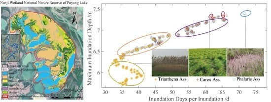
3.2. Hydrological Drivers for the Spatial Distribution of Wetland Herbaceous Communities

The spatial variations of the four hydrological conditions in the NWNNR study area are displayed in Figure 4. The step sizes (intervals) of AIDU, IDUI, AIDE, and MIDE were specified as 10 days, 5 days, 0.05 m, and 0.02 m, respectively. The AIDU was 183 days on average, with a range from 105 to 273 days, where 120~130 days of inundation duration per year was the most frequent result (Figure 5a). The IDUI was 32~88 days, with durations between 35 and 40 days being the most frequent (Figure 5b). The AIDE ranged from 1.42 to 2.01 m, averaging 1.58 m, with the widest area fraction of 1.5~1.55 days (Figure 5c). The MIDE varied from 5.65 to 7.75 m, with the most frequent maximum inundation depth of 5.9 to 6.1 m (Figure 5d), closely related to the elevation distribution characteristics of the study area.
The biplot of the CCA separated the three vegetation communities in different zones (Figure 6). The ordination axes 1 and 2 cumulatively explained 59.2% of the variances in the species and environment. Statistical variables associated with inundation duration and depth already captured most species distribution variations. The CCA showed that the percentage of the cumulative variance of the first axis was 41.91%, accounting for 70.83% of the information regarding the relationships between species and environments. In the CCA biplots, axis 1 was negatively correlated with the AIDU, IDUI, AIDE, and MIDE, which mainly represented a decreasing inundation condition from left to right. Triarrhena Ass was distributed in the right part of the biplot, with shallow inundation depth and duration, and was clearly distinguished from Carex Ass and Phalaris Ass. Axis 2 was strongly positively correlated with the four hydrological indices, representing a decreasing inundation condition from the bottom to the top. Phalaris Ass was at the upper left part of the biplot and was further separated from Carex Ass by its inundation days.
The area fraction of Phalaris Ass, Carex Ass, and Triarrhena Ass in the study area was calculated for the different levels of hydrological indicators to determine their preference. The results are shown in Figure 7.
Phalaris Ass was mainly located in the downstream part of the study area, at a lower elevation between the lakeshore and the lake center (Figure 3). The average annual inundation days in the space occupied by Phalaris Ass were mainly in the range of 150~240 days (Figure 7a). The maximum area fraction of Phalaris Ass was 53.01%, while the average annual inundation days were between 220 and 230 days. Phalaris Ass only grew in the area with average inundation of 40~70 days per inundation, and mainly in the regions that were inundated for 50~60 days at a time (Figure 7b). The average inundation depth of the space occupied by Phalaris Ass was mainly 1.60 to 1.75 m. The area fraction of Phalaris Ass was greatest at 39.03% when the average inundation depth was 1.60 to 1.65 m. Figure 7c,d show that the annual maximum inundation depth that Phalaris Ass could tolerate was 7.3 m. The Phalaris Ass almost died when the average annual inundation was greater than 240 days or when the average inundation depth was greater than 1.75 m.
Carex Ass was mainly grown at mid-to-upper elevations between the lakeshore and the lake center (Figure 3), adjacent to Triarrhena Ass at higher elevations, and below Phalaris Ass. The average of inundation days per year for the space occupied by Carex Ass was mainly in the range of 120~230 days, with the greatest area fraction of 98.84% when the average number of days of inundation per year was between 160 and 170 days (Figure 7a). For the average inundation time in terms of days per inundation, Carex Ass had a maximum area fraction of 90%, achieved at the segment of 30~35 days (Figure 7b). The average inundation depth of the space occupied by Carex Ass was mainly 1.5 to 1.7 m. The maximum area fraction of Carex Ass was 45.68% when the average inundation depth was 1.55 to 1.6 m (Figure 7c). Carex Ass could also grow in the annual maximum inundation depth of 7.3 m, but the area fraction was lower than that of Phalaris Ass (Figure 7d). Average annual inundation over 230 days or average inundation depth greater than 1.7 m cannot facilitate the normal growth and development of Carex Ass.
Triarrhena Ass was mainly located at higher elevations close to the lakeshore (Figure 3), with Carex Ass beneath. The average annual inundation for the space occupied by Triarrhena Ass was mainly 110~140 days, with the greatest area fraction of 99.71%, while the average annual inundation was 110~120 days (Figure 7a). The average inundation duration per inundation for Triarrhena Ass was shorter than that for other two communities (Figure 7b). It ranged from 30 to 45 days, and there was only a small amount per segment. The average inundation depth of the space occupied by Triarrhena Ass was mainly in the range of 1.4 to 1.55 m, with the greatest area fraction of nearly 100% when the average inundation depth was 1.4 to 1.45 m (Figure 7c). Triarrhena Ass had the lowest annual maximum inundation depth (Figure 7d), and almost ceased to occur when the average annual inundation was greater than 140 days or the average inundation depth was greater than 1.55 m.
A vegetative population’s normal distribution along environmental gradients can be assessed using a Gaussian regression model [24]. However, the statistical results showed that only two cases—i.e., the ADUE and MIDE of Triarrhena Ass—did not fit the Gaussian distribution well. This may originate from Triarrhena Ass growing in the most marginal hydrological niche of the three herbaceous communities. The hydrological niche and ecological optimum of the three plant communities are quantified in Table 2. The statistical results indicate a significant difference in the optimal inundation conditions of different wetland herbaceous communities. The ecological optimum of Phalaris Ass was the largest, followed by Carex Ass, while that of Triarrhena Ass was the smallest.

4. Discussion

In this study, we first used a synchronized optimization algorithm to ensure a more accurate and efficient herbaceous community classification model, and then the relationships between the three plant communities and the four hydrological indicators were analyzed by CCA. Finally, the detailed hydrological niches of the three plant communities were quantified. How the plant communities of the Poyang Lake wetland respond to the different hydrological indicators under this framework still needs to be discussed.
The optimal hydrological niches can indicate the competitive advantage of a vegetation community. For example, the optimal hydrological niches for Carex Ass almost overlapped with those for Phalaris Ass, but there was little overlap with Triarrhena Ass. Phalaris Ass was the most tolerant to inundation depth and duration, while Carex Ass had the widest optimal hydrological niches. This explains the wide distribution area of Carex Ass, while Phalaris Ass grew at the lowest end of the hydrological gradient relative to the other two communities. Carex Ass was able to grow in all other communities’ hydrological conditions, providing further explanation for its wide distribution. The results did not deviate significantly from previous conclusions on suitable hydrological conditions derived from controlled experiments or field surveys [28,80]. The authors of [28] also found that the optimal AIDU and AIDE of the Carex community were greater than those of the Phragmites community.
Of the four factors examined by CCA, MIDE and IDUI best explained the distribution of plant communities and were the least correlated. From the perspective of the plants’ adaptation strategy in response to flooding, MIDE and IDUI can adequately characterize the hydrological niches of the three plant communities. In contrast, AIDU and AIDE interpret the hydrological factors purely from a statistical point of view, while MIDE and IDUI can directly affect the survival of plants. In addition, the hydrological conditions most conducive to the growth and reproduction of wetland plants vary throughout the year and at different stages of growth [9]. Desiccation and inundation tolerance determine the distribution of many plant communities along the aquatic–terrestrial transition zones [81]. Since it is difficult to tolerate long-term and deep root submersion, the low flood stage promotes the growth of Triarrhena Ass [82]. In contrast, Carex Ass and Phalaris Ass grow best on exposed sites with wet soils. Under normal summer flood conditions, the plants are submerged and dormant [83]. Wetland plants have gradually evolved a range of biological traits and life-history strategies to cope with specific rhythms of water level fluctuations during long-term adaptation, and vegetation communities will continue to adjust to future long-term changes in lakes’ hydrological conditions [84,85,86].
For floodplains, hydrological conditions are a vital determinant of wetland herbaceous communities’ overall biomass and spatial distribution [87,88]. However, it should be noted that several other factors—such as soil [89], microtopography [49,90], and water table [91]—can also influence vegetation by altering the available water. Thus, vegetation competes intraspecifically and interspecifically for readily available water sources. For example, soil compaction and physical abrasion appear to favor stress-tolerant root plants over shrubs and more sensitive perennials [90,92]. On the other hand, the response of plant communities to flooding is affected by the bioecological characteristics of the species in question [37]. Fluctuations in water levels can affect the growth of individual species (i.e., weaker or stronger competitive advantage) and, thus, change the species’ relationships. In order to fully grasp the distribution principles of vegetation in this changing habitat, the focus of later research should involve interspecific and intraspecific relationships.
The hydrological situation of Poyang Lake is influenced by many external factors, such as the discharge levels of the Yangtze River, its five major tributaries, and its upstream reservoirs [52,93]. Moreover, most of the sub-lakes of Poyang Lake are under artificial control by dams [94]. These sub-lakes are submerged during summer floods and detached from the main body of the lake during the fall months as the lake stage declines and the lake extent shrinks. Shallow water in these sub-lakes during the late fall and winter months provides an ideal habitat for aquatics and migratory waterbirds. Therefore, if the hydrological variation of the Poyang Lake is clearly described, artificial control of sub-lakes can be used to regulate the fluctuation of water levels to meet the growing demand of the plant communities and migratory birds. In future studies, adding a hydrodynamic model and assessing the spatiotemporal fluctuations via remote sensing (e.g., inundation mapping using satellite-based techniques) can provide further insights into the hydrology–vegetation relationships. To this end, the fine topography—especially the artificial control of sub-lakes—needs to be further incorporated to improve the analytical framework.

5. Conclusions

This study established a framework that integrates machine-learning-based methods for plant community classification and quantitative analysis of hydrological niches of the communities. The framework was used to study the relationships between wetland herbaceous community distribution and the hydrological regimes of Poyang Lake. The following conclusions can be drawn:
(1)
Support-vector classification with an input/parameter-synchronized optimization is beneficial for constructing an accurate wetland herbaceous vegetation classification model. The optimized model improved the classification accuracy by ~8% compared with the classic SVM.
(2)
Significant interspecific differences were found in terms of the hydrological niche. Carex Ass was the most adaptable to the duration of inundation, had the widest distribution range, and had a larger hydrological niche amplitude. Triarrhena Ass was the least capable and had the smallest hydrological niche amplitude. The main reasons for the interspecific differences were the different survival strategies of species in the face of inundation, such as dormancy and biological traits.
(3)
The analytical framework was successfully applied to identify key indicators characterizing plant communities’ distribution and quantifying the hydrological niches/optima of the communities in the Poyang Lake wetland.
Our integrated analytical framework could contribute to hydrological management design to better protect the wetland plant community structure in Poyang Lake and, implicitly, in comparable global wetland ecosystems.

Author Contributions

Conceptualization, W.H., T.H., J.M., and H.D.; methodology, W.H. and T.H.; resources, S.W., J.L., and J.Y.; software, W.H. and T.H.; validation, T.H. and J.M.; formal analysis, W.H.; investigation, W.H., T.H., S.W., J.L., and J.Y.; writing—original draft preparation, W.H.; writing—review and editing, T.H., C.M., and R.B.; visualization, W.H. and T.H.; supervision, J.M., C.M., R.B., and H.D. All authors have read and agreed to the published version of the manuscript.

Funding

This research was funded by the National Key Research and Development Program of China (2021YFC3200301), the National Natural Science Foundation of China (51909168), and the Science and Technology Program of Chongqing Transportation Bureau (2020-07).

Data Availability Statement

The data presented in this study are available on request from the corresponding author.

Acknowledgments

The constructive suggestions from the anonymous reviewers are gratefully acknowledged. Thanks to Yifan Xu from Nanjing Hydraulic Research Institute for his help with revising the manuscript. We gratefully acknowledge European Copernicus Satellite Program for providing free access to Sentinel-2 data. Special thanks to China Scholarship Council (CSC).

Conflicts of Interest

The authors declare no conflict of interest.

Appendix A

Table A1. Multispectral indices used in this study.
IndicesFormula (Sentinel-2)References
DVI-Difference Vegetation Index B 8 B 4 [95]
RVI-Ratio Vegetation Index B 8 / B 4 [96]
NDVI- Normalized Difference Vegetation Index B 8 B 4 B 8 + B 4 [97]
EVI—Enhanced Vegetation Index 2 . 5 × ( B 8 B 4 ) B 8 + 6 × B 4 7.5 × B 2 + 1 [98]
MSAVI—Modified Soil Adjusted Vegetation Index 2 B 8 + 1 ( 2 B 8 + 1 ) 2 8 ( B 8 B 4 ) 2 [99]
RDVI—Renormalized Difference Vegetation Index B 8 B 4 B 8 + B 4 ( B 8 B 4 ) [100]
HJVI—Huan Jing Vegetation Index 2 ( B 8 B 4 ) B 3 7.5 B 2 + 0.9 [101]
ARVI -Atmospherically Resistant Vegetation Index B 8 ( 2 B 4 B 2 ) B 8 + ( 2 B 4 B 2 ) [102]
VDVI—Visible-band Difference Vegetation Index 2 B 3 B 4 B 2 2 B 3 + B 4 + B 2 [103]
NGRDI—Normalized Green and Red Difference Vegetation Index B 3 B 4 B 3 + B 4 [104]
NGBDI—Normalized Green and Bule Difference Vegetation Index B 3 B 2 B 3 + B 2 [105]
NDVIre1—Normalized Difference Vegetation Index red-edge 1 B 8 B 5 B 8 + B 5 [106]
NDVIre1n—Normalized Difference Vegetation Index red-edge 1 narrow B 8 a B 5 B 8 a + B 5 [107]
NDVIre2—Normalized Difference Vegetation Index red-edge 2 B 8 B 6 B 8 + B 6 [106]
NDVIre2n—Normalized Difference Vegetation Index red-edge 2 narrow B 8 a B 7 B 8 a + B 7 [107]
NDVIre3—Normalized Difference Vegetation Index red-edge 3 B 8 B 7 B 8 + B 7 [106]
NDVIre3n—Normalized Difference Vegetation Index red-edge 3 narrow B 8 a B 7 B 8 a + B 7 [107]
PSRI—Plant Senescence Reflectance Index B 4 B 3 B 6 [108]
CIre—ChlorophyerII Index red-edge B 7 B 5 1 [109]
NDre1—Normalized Difference red-edge1 B 6 B 5 B 6 + B 5 [106]
Table A2. Genetic algorithm parameter setting and search boundaries for the plant community classification model.
SubjectParameterValue
Genetic AlgorithmMaximum number of function calls4000
Normalized Geometric SelectionSelecting the best individual probability0.05
Simple Crossover--
Arithmetic Crossover--
Heuristic CrossoverNumber of retries10
Uniform Variation--
Non-Uniform VariationShape parameters3
Multiple Non-Uniform VariationShape parameters3
Boundary Variation--
Search BoundariesC lower boundary1
C upper boundary1 × 1012
γ lower boundary1 × 10−2
γ upper boundary1 × 104
Table A3. Accuracy matrix of the training/validation set.
WaterSandPhalaris AssCarex AssTriarrhena AssMudflatUA(%)
Water3721/272421/300/00/00/00/099.44/99.20
Sand13/222671/27890/00/00/02/1099.44/98.87
Phalaris Ass0/00/02516/247050/8115/917/3896.84/95.07
Carex Ass0/00/070/695693/58064/34/798.65/98.66
Triarrhena Ass0/00/020/270/21584/16370/098.75/98.26
Mudflat0/012/1520/381/20/02625/278898.76/98.07
PA(%)99.65/99.4198.78/98.4195.81/94.8599.11/98.5698.81/99.2799.13/98.07OA = 98.69/98.20
Figure A1. Simulation of (a) the wetland herbaceous communities’ distribution and (b) a drone RGB image in Chuankuijia village.
Remotesensing 14 04870 g0a1

References

  1. Casanova, M.T.; Brock, M.A. How do depth, duration and frequency of flooding influence the establishment of wetland plant communities? Plant Ecol. 2000, 147, 237–250. [Google Scholar] [CrossRef]
  2. Bunn, S.E.; Arthington, A.H. Basic principles and ecological consequences of altered flow regimes for aquatic biodiversity. Environ. Manag. 2002, 30, 492–507. [Google Scholar] [CrossRef] [PubMed]
  3. Keddy, P.A. Wetland Ecology: Principles and Conservation, 2nd ed.; Cambridge University Press: Cambridge, UK, 2010. [Google Scholar]
  4. Wilcox, D.A.; Nichols, S.J. The effects of water-level fluctuations on vegetation in a Lake Huron wetland. Wetlands 2008, 28, 487–501. [Google Scholar] [CrossRef]
  5. Todd, M.J.; Muneepeerakul, R.; Pumo, D.; Azaele, S.; Miralles-Wilhelm, F.; Rinaldo, A.; Rodriguez-Iturbe, I. Hydrological drivers of wetland vegetation community distribution within Everglades National Park, Florida. Adv. Water Resour. 2010, 33, 1279–1289. [Google Scholar] [CrossRef]
  6. Zhang, Q.; Ye, X.-C.; Werner, A.D.; Li, Y.-L.; Yao, J.; Li, X.-H.; Xu, C.-Y. An investigation of enhanced recessions in Poyang Lake: Comparison of Yangtze River and local catchment impacts. J. Hydrol. 2014, 517, 425–434. [Google Scholar] [CrossRef]
  7. Tang, X.; Li, H.; Xu, X.; Yang, G.; Liu, G.; Li, X.; Chen, D. Changing land use and its impact on the habitat suitability for wintering Anseriformes in China’s Poyang Lake region. Sci. Total Environ. 2016, 557, 296–306. [Google Scholar]
  8. Liang, D.; Lu, J.; Chen, X.; Liu, C.; Lin, J. An investigation of the hydrological influence on the distribution and transition of wetland cover in a complex lake–floodplain system using time-series remote sensing and hydrodynamic simulation. J. Hydrol. 2020, 587, 125038. [Google Scholar] [CrossRef]
  9. Wan, R.; Dai, X.; Shankman, D. Vegetation response to hydrological changes in Poyang Lake, China. Wetlands 2018, 39, 99–112. [Google Scholar] [CrossRef]
  10. Mei, X.; Dai, Z.; Fagherazzi, S.; Chen, J. Dramatic variations in emergent wetland area in China’s largest freshwater lake, Poyang Lake. Adv. Water Resour. 2016, 96, 1–10. [Google Scholar] [CrossRef]
  11. Han, X.; Chen, X.; Feng, L. Four decades of winter wetland changes in Poyang Lake based on Landsat observations between 1973 and 2013. Remote Sens. Environ. 2015, 156, 426–437. [Google Scholar] [CrossRef]
  12. Mu, S.; Yang, G.; Xu, X.; Wan, R.; Li, B. Assessing the inundation dynamics and its impacts on habitat suitability in Poyang Lake based on integrating Landsat and MODIS observations. Sci. Total Environ. 2022, 834, 154936. [Google Scholar] [CrossRef] [PubMed]
  13. Dai, X.; Wan, R.; Yang, G.; Wang, X.; Xu, L. Responses of wetland vegetation in Poyang Lake, China to water-level fluctuations. Hydrobiologia 2016, 773, 35–47. [Google Scholar] [CrossRef]
  14. Xia, S.; Liu, Y.; Wang, Y.; Chen, B.; Jia, Y.; Liu, G.; Yu, X.; Wen, L. Wintering waterbirds in a large river floodplain: Hydrological connectivity is the key for reconciling development and conservation. Sci. Total Environ. 2016, 573, 645–660. [Google Scholar] [CrossRef] [PubMed]
  15. Tamisier, A.; Grillas, P. A review of habitat changes in the Camargue: An assessment of the effects of the loss of biological diversity on the wintering waterfowl community. Biol. Conserv. 1994, 70, 39–47. [Google Scholar] [CrossRef]
  16. Wang, H.F.; Ren, M.X.; López-Pujol, J.; Ross Friedman, C.; Fraser, L.H.; Huang, G.X. Plant species and communities in Poyang Lake, the largest freshwater lake in China. Collect. Bot. 2015, 34, e004. [Google Scholar]
  17. Hu, Z.P.; Ge, G.; Liu, C.L.; Chen, F.S.; Li, S. Structure of Poyang Lake wetland plants ecosystem and influence of lake water level for the structure. Resour. Environ. Yangtze Basin 2010, 19, 597–605. [Google Scholar]
  18. Fan, H.; Xu, L.; Wang, X.; Jiang, J.; Feng, W.; You, H. Relationship between vegetation community distribution patterns and environmental factors in typical wetlands of Poyang Lake, China. Wetlands 2019, 39, 75–87. [Google Scholar] [CrossRef]
  19. Kumari, N.; Srivastava, A.; Kumar, S. Hydrological Analysis Using Observed and Satellite-Based Estimates: Case Study of a Lake Catchment in Raipur, India. J. Indian Soc. Remote Sens. 2022, 50, 115–128. [Google Scholar] [CrossRef]
  20. Mahdavi, S.; Salehi, B.; Granger, J.; Amani, M.; Brisco, B.; Huang, W. Remote sensing for wetland classification: A comprehensive review. GIScience Remote Sens. 2018, 55, 623–658. [Google Scholar] [CrossRef]
  21. Guo, M.; Li, J.; Sheng, C.; Xu, J.; Wu, L. A Review of Wetland Remote Sensing. Multidiscip. Digit. Publ. Inst. 2017, 17, 777. [Google Scholar] [CrossRef]
  22. Dronova, I. Object-Based Image Analysis in Wetland Research: A Review. Remote Sens. 2015, 7, 6380–6413. [Google Scholar] [CrossRef]
  23. Huang, C.; Davis, L.S.; Townshend, J.R.G. An assessment of support vector machines for land cover classification. Int. J. Remote Sens. 2002, 23, 725–749. [Google Scholar] [CrossRef]
  24. Chen, Y.; Niu, Z.; Johnston, C.A.; Hu, S. A Unifying Approach to Classifying Wetlands in the Ontonagon River Basin, Michigan, Using Multi_temporal Landsat_8 OLI Imagery. Can. J. Remote Sens. 2018, 44, 373–389. [Google Scholar] [CrossRef]
  25. Xu, P.; Niu, Z.; Tang, P. Comparison and assessment of NDVI time series for seasonal wetland classification. Int. J. Digit. Earth 2018, 11, 1103–1131. [Google Scholar] [CrossRef]
  26. Wang, L.; Dronova, I.; Gong, P.; Yang, W.; Li, Y.; Liu, Q. A new time series vegetation–water index of phenological–hydrological trait across species and functional types for Poyang Lake wetland ecosystem. Remote Sens. Environ. 2012, 125, 49–63. [Google Scholar] [CrossRef]
  27. Zhang, C.; Xie, Z. Object-based Vegetation Mapping in the Kissimmee River Watershed Using HyMap Data and Machine Learning Techniques. Wetlands 2013, 33, 233–244. [Google Scholar] [CrossRef]
  28. Zhiqiang, T.; Qi, Z.; Mengfan, L.; Yunliang, L.; Xiuli, X.; Jiahu, J. A study of the relationship between wetland vegetation communities and water regimes using a combined remote sensing and hydraulic modeling approach. Hydrol. Res. 2016, 47, 278–292. [Google Scholar] [CrossRef]
  29. Han, X.; Feng, L.; Hu, C.; Chen, X. Wetland changes of China’s largest freshwater lake and their linkage with the Three Gorges Dam. Remote Sens. Environ. 2018, 204, 799–811. [Google Scholar] [CrossRef]
  30. Li, C.; Wang, J.; Wang, L.; Hu, L.; Gong, P. Comparison of classification algorithms and training sample sizes in urban land classification with Landsat thematic mapper imagery. Remote Sens. 2014, 6, 964–983. [Google Scholar] [CrossRef]
  31. Amani, M.; Brisco, B.; Afshar, M.; Mirmazloumi, S.M.; Mahdavi, S.; Mirzadeh, S.M.J.; Huang, W.; Granger, J. A generalized supervised classification scheme to produce provincial wetland inventory maps: An application of Google Earth Engine for big geo data processing. Big Earth Data 2019, 3, 378–394. [Google Scholar] [CrossRef]
  32. Ghorbanian, A.; Kakooei, M.; Amani, M.; Mahdavi, S.; Mohammadzadeh, A.; Hasanlou, M. Improved land cover map of Iran using Sentinel imagery within Google Earth Engine and a novel automatic workflow for land cover classification using migrated training samples. ISPRS J. Photogramm. Remote Sens. 2020, 167, 276–288. [Google Scholar] [CrossRef]
  33. Parmuchi, M.G.; Karszenbaum, H.; Kandus, P. Mapping wetlands using multi-temporal RADARSAT-1 data and a decision-based classifier. Can. J. Remote Sens. 2002, 28, 175–186. [Google Scholar] [CrossRef]
  34. Slatton, K.C.; Crawford, M.M.; Chang, L.-D. Modeling temporal variations in multipolarized radar scattering from intertidal coastal wetlands. ISPRS J. Photogramm. Remote Sens. 2008, 63, 559–577. [Google Scholar] [CrossRef]
  35. Hu, T.; Mao, J.; Pan, S.; Dai, L.; Zhang, P.; Xu, D.; Dai, H. Water level management of lakes connected to regulated rivers: An integrated modeling and analytical methodology. J. Hydrol. 2018, 562, 796–808. [Google Scholar] [CrossRef]
  36. Guan, L.; Wen, L.; Feng, D.; Zhang, H.; Lei, G. Delayed flood recession in central Yangtze floodplains can cause significant food shortages for wintering geese: Results of inundation experiment. Environ. Manag. 2014, 54, 1331–1341. [Google Scholar] [CrossRef]
  37. Foti, R.; del Jesus, M.; Rinaldo, A.; Rodriguez-Iturbe, I. Hydroperiod regime controls the organization of plant species in wetlands. Proc. Natl. Acad. Sci. USA 2012, 109, 19596–19600. [Google Scholar] [CrossRef]
  38. David, P.G. Changes in plant communities relative to hydrologic conditions in the Florida Everglades. Wetlands 1996, 16, 15–23. [Google Scholar] [CrossRef]
  39. Zhang, Q.; Sun, P.; Chen, X.; Jiang, T. Hydrological extremes in the Poyang Lake basin, China: Changing properties, causes and impacts. Hydrol. Process. 2011, 25, 3121–3130. [Google Scholar] [CrossRef]
  40. Craine, J.M.; Dybzinski, R. Mechanisms of plant competition for nutrients, water and light. Funct. Ecol. 2013, 27, 833–840. [Google Scholar] [CrossRef]
  41. Keddy, P.; Reznicek, A. Great Lakes vegetation dynamics: The role of fluctuating water levels and buried seeds. J. Great Lakes Res. 1986, 12, 25–36. [Google Scholar] [CrossRef]
  42. Riis, T.; Hawes, I. Relationships between water level fluctuations and vegetation diversity in shallow water of New Zealand lakes. Aquat. Bot. 2002, 74, 133–148. [Google Scholar] [CrossRef]
  43. Zhang, L.; Yin, J.; Jiang, Y.; Wang, H. Relationship between the hydrological conditions and the distribution of vegetation communities within the Poyang Lake National Nature Reserve, China. Ecol. Inform. 2012, 11, 65–75. [Google Scholar] [CrossRef]
  44. Silvertown, J.; Dodd, M.E.; Gowing, D.J.G.; Mountford, J.O. Hydrologically defined niches reveal a basis for species richness in plant communities. Nature 1999, 400, 61–63. [Google Scholar] [CrossRef]
  45. Magee, T.K.; Kentula, M.E. Response of wetland plant species to hydrologic conditions. Wetl. Ecol. Manag. 2005, 13, 163–181. [Google Scholar] [CrossRef]
  46. Ma, S.; Ren, J.; Wu, C.; Cheng, F.; Wang, X.; Li, B.; He, Q. Hydrological control of threshold transitions in vegetation over early-period wetland development. J. Hydrol. 2022, 610, 127931. [Google Scholar] [CrossRef]
  47. Silvertown, J.; Araya, Y.N.; Gowing, D. Hydrological niches in terrestrial plant communities: A review. J. Ecol. 2015, 103, 93–108. [Google Scholar] [CrossRef]
  48. Liao, F.; Wang, G.; Yi, L.; Shi, Z.; Cheng, G.; Kong, Q.; Mu, W.; Guo, L.; Cheng, K.; Dong, N.; et al. Applying radium isotopes to estimate groundwater discharge into Poyang Lake, the largest freshwater lake in China. J. Hydrol. 2020, 585, 124782. [Google Scholar] [CrossRef]
  49. Zheng, L.; Wang, X.; Li, D.; Xu, G.; Guo, Y. Spatial heterogeneity of vegetation extent and the response to water level fluctuations and micro-topography in Poyang Lake, China. Ecol. Indic. 2021, 124, 107420. [Google Scholar] [CrossRef]
  50. Lai, X.; Huang, Q.; Zhang, Y.; Jiang, J. Impact of lake inflow and the Yangtze River flow alterations on water levels in Poyang Lake, China. Lake Reserv. Manag. 2014, 30, 321–330. [Google Scholar] [CrossRef]
  51. Hu, Z.; Zhang, Z.; Liu, Y.; Ji, W.; Ge, G. The function and significance of the Shallow-Lakes in the Poyang Lake wetland ecosystem. Jiangxi Hydraul. Sci. Technol. 2015, 41, 317–323. [Google Scholar]
  52. Liu, X.; Zhang, Q.; Li, Y.; Tan, Z.; Werner, A.D. Satellite image-based investigation of the seasonal variations in the hydrological connectivity of a large floodplain (Poyang Lake, China). J. Hydrol. 2020, 585, 124810. [Google Scholar] [CrossRef]
  53. Shen, R.; Lan, Z.; Huang, X.; Chen, Y.; Hu, Q.; Fang, C.; Jin, B.; Chen, J. Soil and plant characteristics during two hydrologically contrasting years at the lakeshore wetland of Poyang Lake, China. J. Soils Sediments 2020, 20, 3368–3379. [Google Scholar] [CrossRef]
  54. Yao, J.; Zhang, Q.; Li, Y.; Li, M. Hydrological evidence and causes of seasonal low water levels in a large river-lake system: Poyang Lake, China. Hydrol. Res. 2016, 47, 24–39. [Google Scholar] [CrossRef]
  55. Dronova, I.; Gong, P.; Wang, L.; Zhong, L. Mapping dynamic cover types in a large seasonally flooded wetland using extended principal component analysis and object-based classification. Remote Sens. Environ. 2015, 158, 193–206. [Google Scholar] [CrossRef]
  56. Shankman, D.; Keim, B.D. Flood risk forecast for China’s Poyang Lake region. Phys. Geogr. 2016, 37, 88–91. [Google Scholar] [CrossRef]
  57. Liu, X.Z.; Fan, S.B.; Hu, B.H. Comprehensive and Scientific Survey of Jiangxi Nanjishan Wetland Nature Reserve; China Foresry Press: Beijing, China, 2006. [Google Scholar]
  58. Kettenring, K.; Gardner, G.; Galatowitsch, S.M. Effect of light on seed germination of eight wetland Carex species. Ann. Bot. 2006, 98, 869–874. [Google Scholar] [CrossRef]
  59. Chen, X.-S.; Deng, Z.-M.; Xie, Y.-H.; Li, F.; Hou, Z.-Y.; Li, X. Belowground bud banks of four dominant macrophytes along a small-scale elevational gradient in Dongting Lake wetlands, China. Aquat. Bot. 2015, 122, 9–14. [Google Scholar] [CrossRef]
  60. Huang, Y.; Chen, X.-S.; Zou, Y.-A.; Zhang, P.-Y.; Li, F.; Hou, Z.-Y.; Li, X.; Zeng, J.; Deng, Z.-M.; Zhong, J.-R.; et al. Exploring the relative contribution of flood regimes and climatic factors to Carex phenology in a Yangtze River-connected floodplain wetland. Sci. Total Environ. 2022, 847, 157568. [Google Scholar] [CrossRef] [PubMed]
  61. Xia, S.; Wang, Y.; Lei, G.; Liu, Y.; Lei, J.; Yu, X.; Wen, L.; Zhou, Y. Restriction of herbivorous waterbird distributions in the middle and lower Yangtze River floodplain in view of hydrological isolation. Wetlands 2017, 37, 79–88. [Google Scholar] [CrossRef]
  62. Ming-Qin, S.; Hong, G. Population sizes and group characteristics of Siberian crane (Leucogeranus leucogeranus) and hooded crane (Grus monacha) in Poyang Lake Wetland. Zool. Res. 2014, 35, 373. [Google Scholar]
  63. ESA. Sentinel-2 User Handbook; ESA Standard Document; ESA-Star Publication: Paris, France, 2015; Volume 64, pp. 1–64. [Google Scholar]
  64. Kaplan, G.; Avdan, U. Evaluating Sentinel-2 Red-Edge Bands for Wetland Classification. Proceedings 2019, 18, 12. [Google Scholar]
  65. Rupasinghe, P.A.; Chow-Fraser, P. Identification of most spectrally distinguishable phenological stage of invasive Phramites australis in Lake Erie wetlands (Canada) for accurate mapping using multispectral satellite imagery. Wetl. Ecol. Manag. 2019, 27, 513–538. [Google Scholar] [CrossRef]
  66. Amani, M.; Kakooei, M.; Ghorbanian, A.; Warren, R.; Mahdavi, S.; Brisco, B.; Moghimi, A.; Bourgeau-Chavez, L.; Toure, S.; Paudel, A.; et al. Forty Years of Wetland Status and Trends Analyses in the Great Lakes Using Landsat Archive Imagery and Google Earth Engine. Remote Sens. 2022, 14, 3778. [Google Scholar] [CrossRef]
  67. Rosenfield, G.H.; Fitzpatrick-Lins, K. A coefficient of agreement as a measure of thematic classification accuracy. Photogramm. Eng. Remote Sens. 1986, 52, 223–227. [Google Scholar]
  68. Congalton, R.G. A review of assessing the accuracy of classifications of remotely sensed data. Remote Sens. Environ. 1991, 37, 35–46. [Google Scholar] [CrossRef]
  69. Gause, G. The influence of ecological factors on the size of population. Am. Nat. 1931, 65, 70–76. [Google Scholar] [CrossRef]
  70. Mountrakis, G.; Im, J.; Ogole, C. Support vector machines in remote sensing: A review. ISPRS J. Photogramm. Remote Sens. 2011, 66, 247–259. [Google Scholar] [CrossRef]
  71. Vapnik, V.N. Statistical Learning Theory; John Wiley & Sons, Inc.: New York, NY, USA, 1998. [Google Scholar]
  72. Maryantika, N.; Lin, C. Exploring changes of land use and mangrove distribution in the economic area of Sidoarjo District, East Java using multi-temporal Landsat images(Article). Inf. Process. Agric. 2017, 4, 321–332. [Google Scholar] [CrossRef]
  73. Yang, L.; Wang, L.; Yu, D.; Yao, R.; Li, C.; He, Q.; Wang, S.; Wang, L. Four decades of wetland changes in Dongting Lake using Landsat observations during 1978–2018. J. Hydrol. 2020, 587, 124954. [Google Scholar] [CrossRef]
  74. Keramitsoglou, I.; Sarimveis, H.; Kiranoudis, C.T.; Kontoes, C.; Sifakis, N.; Fitoka, E. The performance of pixel window algorithms in the classification of habitats using VHSR imagery. ISPRS J. Photogramm. Remote Sens. 2006, 60, 225–238. [Google Scholar] [CrossRef]
  75. Wang, M.; Fei, X.; Zhang, Y.; Chen, Z.; Wang, X.; Tsou, J.Y.; Liu, D.; Lu, X. Assessing texture features to classify coastal wetland vegetation from high spatial resolution imagery using completed local binary patterns (CLBP). Remote Sens. 2018, 10, 778. [Google Scholar] [CrossRef]
  76. Giuliani, G.; Egger, E.; Italiano, J.; Poussin, C.; Richard, J.-P.; Chatenoux, B. Essential variables for environmental monitoring: What are the possible contributions of earth observation data cubes? Data 2020, 5, 100. [Google Scholar] [CrossRef]
  77. Pillsbury, F.C.; Miller, J.R. Habitat and landscape characteristics underlying anuran community structure along an urban–rural gradient. Ecol. Appl. 2008, 18, 1107–1118. [Google Scholar] [CrossRef] [PubMed]
  78. Xu, X.; Zhang, Q.; Tan, Z.; Li, Y.; Wang, X. Effects of water-table depth and soil moisture on plant biomass, diversity, and distribution at a seasonally flooded wetland of Poyang Lake, China. Chin. Geogr. Sci. 2015, 25, 739–756. [Google Scholar] [CrossRef]
  79. Yang, X.-D.; Dong, X.-H.; Gao, G.; Pan, H.-X.; Wu, J.-L. Relationship between surface sediment diatoms and summer water quality in shallow lakes of the middle and lower reaches of the Yangtze River. J. Integr. Plant Biol. 2005, 47, 153–164. [Google Scholar] [CrossRef]
  80. Han, Z.; Wang, S.; Liu, X.; Peng, W.; Ge, G.; Huang, A. Ecological thresholds for the dominated wetland plants of Poyang Lake along the gradient of flooding duration. J. Hydraul. Eng. 2019, 50, 252–262. [Google Scholar]
  81. Coops, H.; Beklioglu, M.; Crisman, T.L. The role of water-level fluctuations in shallow lake ecosystems—Workshop conclusions. Hydrobiologia 2003, 506, 23–27. [Google Scholar] [CrossRef]
  82. Deegan, B.M.; White, S.D.; Ganf, G.G. The influence of water level fluctuations on the growth of four emergent macrophyte species. Aquat. Bot. 2007, 86, 309–315. [Google Scholar] [CrossRef]
  83. Schütz, W. Dormancy characteristics and germination timing in two alpine Carex species. Basic Appl. Ecol. 2002, 3, 125–134. [Google Scholar] [CrossRef]
  84. Visser, E.J.W.; Bögemann, G.M.; VAN DE Steeg, H.M.; Pierik, R.; Blom, C.W.P.M. Flooding tolerance of Carex species in relation to field distribution and aerenchyma formation. New Phytol. 2000, 148, 93–103. [Google Scholar] [CrossRef]
  85. Lytle, D.A.; Poff, N.L. Adaptation to natural flow regimes. Trends Ecol. Evol. 2004, 19, 94–100. [Google Scholar] [CrossRef]
  86. Deng, Z.; Xie, Y.; Chen, X.; Li, F.; Hu, C.; Liu, N. Effect of clone size on submergence tolerance and post-submergence growth recovery in Carex brevicuspis (Cyperaceae). J. Limnol. 2017, 76, 424–430. [Google Scholar] [CrossRef]
  87. Mitsch, W.J.; Gosselink, J.G. Wetlands, 5th ed.; Wiley: Hoboken, NJ, USA, 2015; p. 456. [Google Scholar]
  88. Yuan, S.; Yang, Z.; Liu, X.; Wang, H. Key parameters of water level fluctuations determining the distribution of Carex in shallow lakes. Wetlands 2017, 37, 1005–1014. [Google Scholar] [CrossRef]
  89. Castelli, R.M.; Chambers, J.C.; Tausch, R.J. Soil-plant relations along a soil-water gradient in Great Basin riparian meadows. Wetlands 2000, 20, 251–266. [Google Scholar]
  90. Solon, J.; Degórski, M.; Roo-Zielińska, E. Vegetation response to a topographical-soil gradient. Catena 2007, 71, 309–320. [Google Scholar] [CrossRef]
  91. Palanisamy, B.; Chui, T.F.M. Understanding wetland plant dynamics in response to water table changes through ecohydrological modelling. Ecohydrology 2013, 6, 287–296. [Google Scholar] [CrossRef]
  92. Koning, C.O. Vegetation patterns resulting from spatial and temporal variability in hydrology, soils, and trampling in an isolated basin marsh, New Hampshire, USA. Wetlands 2005, 25, 239–251. [Google Scholar] [CrossRef]
  93. Li, Y.; Zhang, Q.; Cai, Y.; Tan, Z.; Wu, H.; Liu, X.; Yao, J. Hydrodynamic investigation of surface hydrological connectivity and its effects on the water quality of seasonal lakes: Insights from a complex floodplain setting (Poyang Lake, China). Sci. Total Environ. 2019, 660, 245–259. [Google Scholar] [CrossRef]
  94. Li, Y.; Zhang, Q.; Liu, X.; Tan, Z.; Yao, J. The role of a seasonal lake groups in the complex Poyang Lake-floodplain system (China): Insights into hydrological behaviors. J. Hydrol. 2019, 578, 124055. [Google Scholar] [CrossRef]
  95. Richardson, A.J.; Wiegand, C.L. Distinguishing vegetation from soil background information. Photogramm. Eng. Remote Sens. 1977, 43, 1541–1552. [Google Scholar]
  96. Pearson, R.L.; Miller, L.D. Remote Mapping of Standing Crop Biomass for Estimation of Productivity of the Shortgrass Prairie. Remote Sens. Environ. 1972, VIII, 1355. [Google Scholar]
  97. Rouse, J.W.; Haas, R.H.; Schell, J.A.; Deering, D.W. Monitoring vegetation systems in the Great Plains with ERTS. NASA Spec. Publ. 1974, 351, 309. [Google Scholar]
  98. Wu, C.; Chen, J.M.; Huang, N. Predicting gross primary production from the enhanced vegetation index and photosynthetically active radiation: Evaluation and calibration. Remote Sens. Environ. 2011, 115, 3424–3435. [Google Scholar] [CrossRef]
  99. Qi, J.; Chehbouni, A.; Huete, A.R.; Kerr, Y.H.; Sorooshian, S. A Modified Soil Adjusted Vegetation Index. Remote Sens. Environ. 1994, 48, 119–126. [Google Scholar] [CrossRef]
  100. Roujean, J.-L.; Breon, F.-M. Estimating PAR absorbed by vegetation from bidirectional reflectance measurements. Remote Sens. Environ. 1995, 51, 375–384. [Google Scholar] [CrossRef]
  101. Zhang, Y.; Meng, Q.-Y.; Wu, J.-L.; Zhao, F. Study of environmental vegetation index based on environment satellite CCD data and LAI inversion. Spectrosc. Spectr. Anal. 2011, 31, 2789–2793. [Google Scholar]
  102. Kaufman, Y.J.; Tanre, D. Atmospherically resistant vegetation index (ARVI) for EOS-MODIS. IEEE Trans. Geosci. Remote Sens. 1992, 30, 261–270. [Google Scholar] [CrossRef]
  103. Wang, X.; Wang, M.; Wang, S.; Wu, Y. Extraction of vegetation information from visible unmanned aerial vehicle images. Trans. Chin. Soc. Agric. Eng. 2015, 31, 152–159. [Google Scholar]
  104. Gitelson, A.A.; Kaufman, Y.J.; Stark, R.; Rundquist, D. Novel algorithms for remote estimation of vegetation fraction. Remote Sens. Environ. 2002, 80, 76–87. [Google Scholar] [CrossRef]
  105. Hunt, E.R.; Cavigelli, M.; Daughtry, C.S.; Mcmurtrey, J.E.; Walthall, C.L. Evaluation of Digital Photography from Model Aircraft for Remote Sensing of Crop Biomass and Nitrogen Status. Precis. Agric. 2005, 6, 359–378. [Google Scholar] [CrossRef]
  106. Gitelson, A.; Merzlyak, M.N. Spectral Reflectance Changes Associated with Autumn Senescence of Aesculus hippocastanum L. and Acer platanoides L. Leaves. Spectral Features and Relation to Chlorophyll Estimation. J. Plant Physiol. 1994, 143, 286–292. [Google Scholar]
  107. Fernández-Manso, A.; Fernández-Manso, O.; Quintano, C. SENTINEL-2A red-edge spectral indices suitability for discriminating burn severity. Int. J. Appl. Earth Obs. Geoinf. 2016, 50, 170–175. [Google Scholar] [CrossRef]
  108. Merzlyak, M.N.; Gitelson, A.A.; Chivkunova, O.B.; Rakitin, V.Y. Non-destructive optical detection of pigment changes during leaf senescence and fruit ripening. Physiol. Plant. 1999, 106, 135–141. [Google Scholar] [CrossRef]
  109. Gitelson, A.A.; Keydan, G.P.; Merzlyak, M.N. Three-band model for noninvasive estimation of chlorophyll, carotenoids, and anthocyanin contents in higher plant leaves. Geophys. Res. Lett. 2006, 33, 431–433. [Google Scholar] [CrossRef] [Green Version]
Figure 1. Map of the study area: (a) locations of the Poyang Lake in the Yangtze River Basin, China; (b) Nanji Wetland National Nature Reserve and Kangshan Station in Poyang Lake; (c) drone image of the area used for training and validation with different land covers.
Remotesensing 14 04870 g001
Figure 2. A flowchart of the integrated analytical framework of hydrological driving factors of the spatial distribution of wetland herbaceous communities. NDVI, EVI, DVI, RVI, and NDre1 are vegetation indices (Table A1). The dashed box represents the synchronous optimization process of input variables and support-vector classification parameters based on a genetic algorithm. Gray blocks indicate the potentially selected parameters.
Remotesensing 14 04870 g002
Figure 3. (a) Model simulation results of wetland plant community distribution and misclassification point distribution. (b) Classification of the wetland plant communities’ distribution in the whole NWNNR area.
Remotesensing 14 04870 g003
Figure 4. Spatial distribution of (a) annual average inundation days (d), (b) average inundation days per inundation (d), (c) annual average inundation depth (m), and (d) annual maximum inundation depth (m) in the study area.
Remotesensing 14 04870 g004
Figure 5. Area fraction of (a) annual average inundation days (d), (b) average inundation days per inundation (d), (c) annual average inundation depth (m), and (d) annual maximum inundation depth (m) in the study area.
Remotesensing 14 04870 g005
Figure 6. Biplot of the final CCA showing the distribution of three vegetation communities along the gradient of the four hydrological indicators in the study area. a—Annual average inundation days (d), b—Average inundation days per inundation (d), c—Annual average inundation depth (m), and d—Annual maximum inundation depth (m).
Remotesensing 14 04870 g006
Figure 7. The area fraction of each plant community based on the statistics of the (a) annual average inundation days (d), (b) average inundation days per inundation (d), (c) annual average inundation depth (m), and (d) annual maximum inundation depth (m) in the study area.
Remotesensing 14 04870 g007
Table 1. Summary of the dominant species and their phenology for the three plant communities.
CommunityPhalaris AssCarex AssTriarrhena Ass
Dominant speciesPhragmites australisCarex cinerascensTriarrhena lutarioriparia, Phragmites australis
Accompanying speciesPotentilla limprichtii, Carex ovatispiculata, and Lapsana apogonoidesPotentilla limprichtii spp., Cardamine lyrata spp., and various Carex spp.Carex cinerascens, Carex argyi, and Polygonum posumbu
Coverage60~80%95~100%85~98%
StructureVertical (two layers)HorizontalVertical (three layers)
PhenologyPerennial herb that sprouts from January to February, blooms before the beginning of the flooding season, and fully develops from April to May [29]. It is submerged during the flood and continues to grow after it recedes until the winter ends [29].Perennial herb with two growing seasons (late spring and mid-autumn) and sprouts in the early spring. It reaches its maximum coverage in April during the first growing season [58]. Generally, they are flooded in the flood season, and a large number of aboveground parts of Carex die or become dormant. The second growing season begins in early autumn when the floodwaters recede, and germination takes place until the maximum coverage is reached, before completely withering in winter [59,60].Blooms from September to October, bears fruit in November, and leaves wither in December [29].
Table 2. The optimal hydrological niche (optimum) of each wetland herbaceous community in the study area.
Phalaris AssCarex AssTriarrhena Ass
Average annual inundation days (d)187~251 (219)132~245 (188.2)107~130 (119.9)
Average inundation days per inundation (d)44~65 (54.7)24~61 (44.3)33~42 (36.5)
Annual average inundation depth (m)1.54~1.76 (1.65)1.50~1.68 (1.58)1.43~1.50 (1.45) *
Annual maximum inundation depth (m)6.58~7.41 (7.00)6.13~7.24 (6.69)5.70~5.99 (5.87) *
* Did not fit the Gaussian distribution well.
Publisher’s Note: MDPI stays neutral with regard to jurisdictional claims in published maps and institutional affiliations.

