Article

Predicting and Mapping Potential Fire Severity for Risk Analysis at Regional Level Using Google Earth Engine

by
Jose Maria Costa-Saura
1,2,*,
Valentina Bacciu
2,3,
Claudio Ribotta
1,
Donatella Spano
1,2,
Antonella Massaiu
4 and
Costantino Sirca
1,2
1
Department of Agricultural Sciences, University of Sassari, 07100 Sassari, Italy
2
Euro-Mediterranean Center on Climate Change Foundation, Impacts on Agriculture, Forests and Ecosystem Services (IAFES) Division, 07100 Sassari, Italy
3
National Research Council of Italy, Institute of Bioeconomy, 07100 Sassari, Italy
4
French National Forest Office, 20090 Ajaccio, France
*
Author to whom correspondence should be addressed.
Remote Sens. 2022, 14(19), 4812; https://doi.org/10.3390/rs14194812
Submission received: 27 May 2022 / Revised: 1 August 2022 / Accepted: 23 September 2022 / Published: 27 September 2022

Abstract

:
Despite being a natural ecological process, wildfires are dramatic events that, accelerated by global change, could negatively affect ecosystem services depending on their severity level. However, because of data processing constraints, fire severity has been mostly neglected in risk analysis (especially at regional levels). Indeed, previous studies addressing fire severity focused mainly on analyzing single fire events, preventing the projection of the results over large areas. Although, building and projecting robust models of fire severity to integrate into risk analysis is of main importance to best anticipate decisions. Here, taking advantage of free data-processing platforms, such as Google Earth Engine, we use more than 1000 fire records from Western Italy and Southern France in the years 2004–2017, to assess the performance of random forest models predicting the relativized delta normalized burn ratio (rdNBR) used as proxy of fire severity. Furthermore, we explore the explanatory capacity and meaning of several variables related to topography, vegetation, and burning conditions. To show the potentialities of this approach for operational purposes, we projected the model for one of the regions (Sardinia) within the study area. Results showed that machine learning algorithms explain up to 75% of the variability in rdNBR, with variables related to vegetation amount and topography being the most important. These results highlight the potential usefulness of these tools for mapping fire severity in risk assessments.

Graphical Abstract

1. Introduction

Global change impacts on ecosystem services are pushing agencies to fund, develop, and implement tools to anticipate decisions for disaster risk reduction (e.g., the European Commission). Despite being a natural ecological process [1,2], wildfires are dramatic events that, accelerated by global change [3,4,5], according to their severity level, could negatively affect the services provided by ecosystems (e.g., water regulation, soil conservation, carbon uptake, or biodiversity) [6]. Previous studies on fire risk, meant as the interaction between hazard, exposure, and vulnerability (sensu IPCC, https://apps.ipcc.ch/glossary/, accessed on 1 March 2022), have been mainly focused on assessing the hazard, i.e., the potential occurrence of wildfires. For instance, fire spread simulators were used to estimate burning probabilities [7,8], machine learning models were calibrated and projected for assessing fire occurrence likelihood [9,10], and climate/weather projections were used to calculate meteorological fire danger across different time scales [11,12]. However, less attention has been put on assessing landscape sensitivity to wildfires. Sensitivity, understood as the degree to which a system is affected by wildfires (sensu IPCC), is a main component of vulnerability. Sensitivity allows analysts to focus on factors modulating the consequences of specific hazards, e.g., the forest characteristics that influence the degree of damage [13,14]. Thus, accounting for sensitivity in wildfire risk analysis might provide a more realistic picture that better contributes to decision making, e.g., allocation of prevention actions.
In wildfire risk assessments, the sensitivity might be represented by fire severity, broadly defined as the magnitude of the environmental effects caused by fires [15], but also, in a more specific sense, as the aboveground and belowground organic matter consumed by fires [16]. Studies addressing fire severity were initially based on field data, thus limiting the number of sample locations and the robustness of results [17]. To overcome such limitations, recent efforts focused on estimating field data through remote sensing to increase the spatial extent of analysis and the frequency of estimations [18,19,20]. Indeed, these studies showed good correlations when using remote sensing indices, such as the normalized burn ratio (NBR) and its relativized difference (rdNBR). The NBR index relies on the fact that burned vegetation does not reflect much within the near infrared (NIR) because of low leaf cover; nevertheless, it reflects a high amount of radiation within the short-wave infrared (SWIR) due to its low moisture content [19]. Thus, good results were observed across climatic regions and vegetation types recognizing the ecological signal provided by rdNBR [21,22,23]. However, the time-consuming judicious selection and downloading–processing of pre-fire and post-fire scenes to calculate rdNBR limited its use to specific fire events. For instance, Viedma et al. [24] and Mitsopoulos et al. [25] assessed factors driving fire severity in Spain and Greece but focusing only on one single fire events. Despite their enormous value for guiding management actions, not fully sampling the whole environmental range prevents their use over larger areas, increasing uncertainties when projecting the models outside the study area [26].
Nowadays, free data and processing platforms, such as Google Earth Engine (GEE), allow the processing of huge amounts of data, overcoming the limitations mentioned earlier. Furthermore, Parks et al., [27] showed how, thanks to GEE, accurate estimations of fire severity can be obtained using mean composite values (i.e., the mean value for NBR over a prespecified data range before and after the fire). It was shown that this procedure saves time, avoiding judicious selection and downloading–processing of fire scenes, also providing better results when relating rdNBR with severity field data. This improvement potentially allows for increasing the number of fire events under analysis and the scale of the study, which, in turn, might increase the robustness of the results. Furthermore, it might allow building of tailored tools for risk analysis accounting for fire sensitivity/vulnerability.
Thus, taking advantage of GEE and the procedure developed by Parks et al. [27], this study uses more than 1000 fire perimeters from Western Italy and Southern France to assess empirical models’ performance when predicting fire severity. Such an approach should overcome the limitations of previous studies in projecting potential fire severity over large areas and might prove helpful for risk analysis. Furthermore, we aim to explore, on a large scale, the effect of variables related with topography, pre-fire vegetation, and burning conditions on fire severity. Finally, as an example of supporting prevention actions under an operational framework, we map the potential fire severity for the region of Sardinia.

2. Materials and Methods
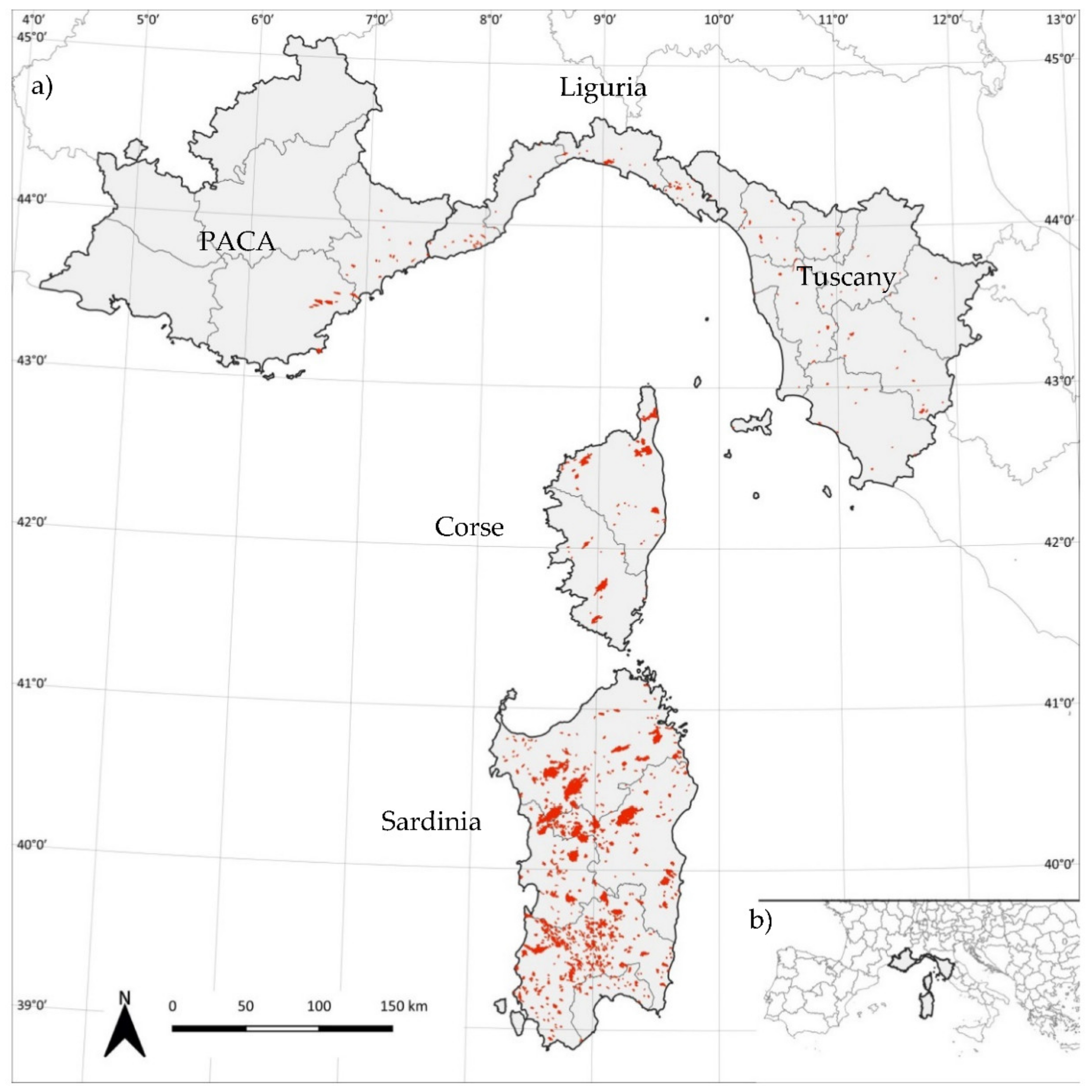
2.1. Study Area

The study area, located in the central Mediterranean basin, covers the French regions of Provence-Alpes-Côte d’Azur (PACA) and Corse, and the Italian regions of Sardinia, Liguria, and Tuscany (Figure 1). The main vegetation types are sclerophyllous shrublands, broadleaf, and coniferous forests (e.g., Quercus ilex and Pinus pinaster, respectively), and agricultural lands interspersed with natural vegetation (Figure 2a). The study area, characterized by a Mediterranean climate, is largely affected by wildfires during the summer season (Figure 2b).

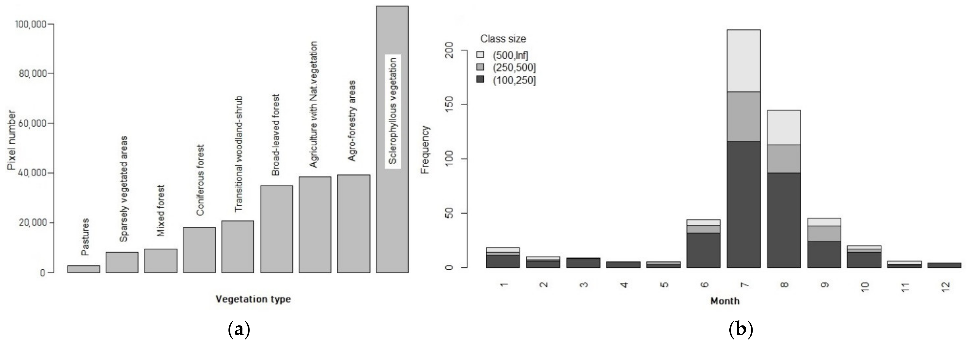
2.2. Fire Perimeters

We used fire perimeters (without excluding inner unburned areas) to extract pixel information regarding fire severity (i.e., rdNBR) and explanatory variables (i.e., topography, vegetation, and burning conditions). Fire perimeters and the date of occurrence were obtained from the French National Forest Office (ONF) and the former Corpo Forestale dello Stato (CFS) for the studied regions in France and Italy, respectively. ONF database only provides data for fires larger than 25 ha (1999–2019), whereas the CFS database covers all fires from 2004 to 2017. For consistency between both datasets, only fires larger than 25 ha and which occurred in 2004–2017 were considered for the analysis. Thus, a total of 1139 fire events were considered. Sardinia was the region recording the most significant number of fire events (84%).

2.3. Fire Severity from Remote Sensing

Fire severity was calculated on GEE using the relativized delta normalized burn ratio (i.e., rdNBR, Equation (2)) following the procedure suggested by Parks et al., [27]. This method, instead of relying on a judicious selection of one pre-fire and one post-fire scene, automatically calculates the mean NBR (Equation (1)) from all the available scenes (i.e., not masked, see below) within a specific data range (i.e., from April to June) for one year before and after the fire event (i.e., NBRprefire and NBRpostfire, respectively). The study from Parks et al. [27] showed that the approach saves time while improving accuracy when validating with field data. rdNBR was preferred over other remote sensing indices (such as dNBR or RBR) presented by Parks et al. [27] because it provides similar levels of accuracy [27]. In addition, as suggested by [19], it is more suitable for analyzing multiple fires in heterogeneous landscapes since it makes comparable pixels with different amounts of vegetation.
N B R = N I R S W I R / N I R + S W I R  
r d N B R = N B R p r e f i r e N B R p o s t f i r e 1000 N B R p r e f i r e 0.5 ,   N B R p r e f i r e 0.001 N B R p r e f i r e N B R p o s t f i r e 1000 0.001 0.5 ,   N B R p r e f i r e < 0.001  
Field data to validate rdNBR as a proxy of fire severity was unavailable for our study area. However, numerous studies already showed the strong relationship between rdNBR and severity field data worldwide [23,27,28] and especially in the Mediterranean region [18,22,24,25,29] (R2 mainly ranging from 0.6 to 0.8). In addition, because of inherent limitations, large-scale studies using NBR as a proxy of fire severity did not perform validation (e.g., [30]), assuming that the strong results from previous studies [18,22,23,24,25,27,28,29] provide enough support for further analysis.
Since fire records started in 2004, rdNBR was calculated using the atmospherically corrected surface reflectance data from Landsat 7 ETM+ (https://developers.google.com/earth-engine/datasets/catalog/LANDSAT_LE07_C01_T1_SR, accessed on 15 December 2021). The dataset, with a spatial and temporal resolution of 30 m and 16 days, respectively, also includes a quality mask, based on the CFMask algorithm [31], to identify pixels with clouds, shadows, water, and snow. Those pixels were excluded for calculating the mean composite pre- and post-fire NBR.

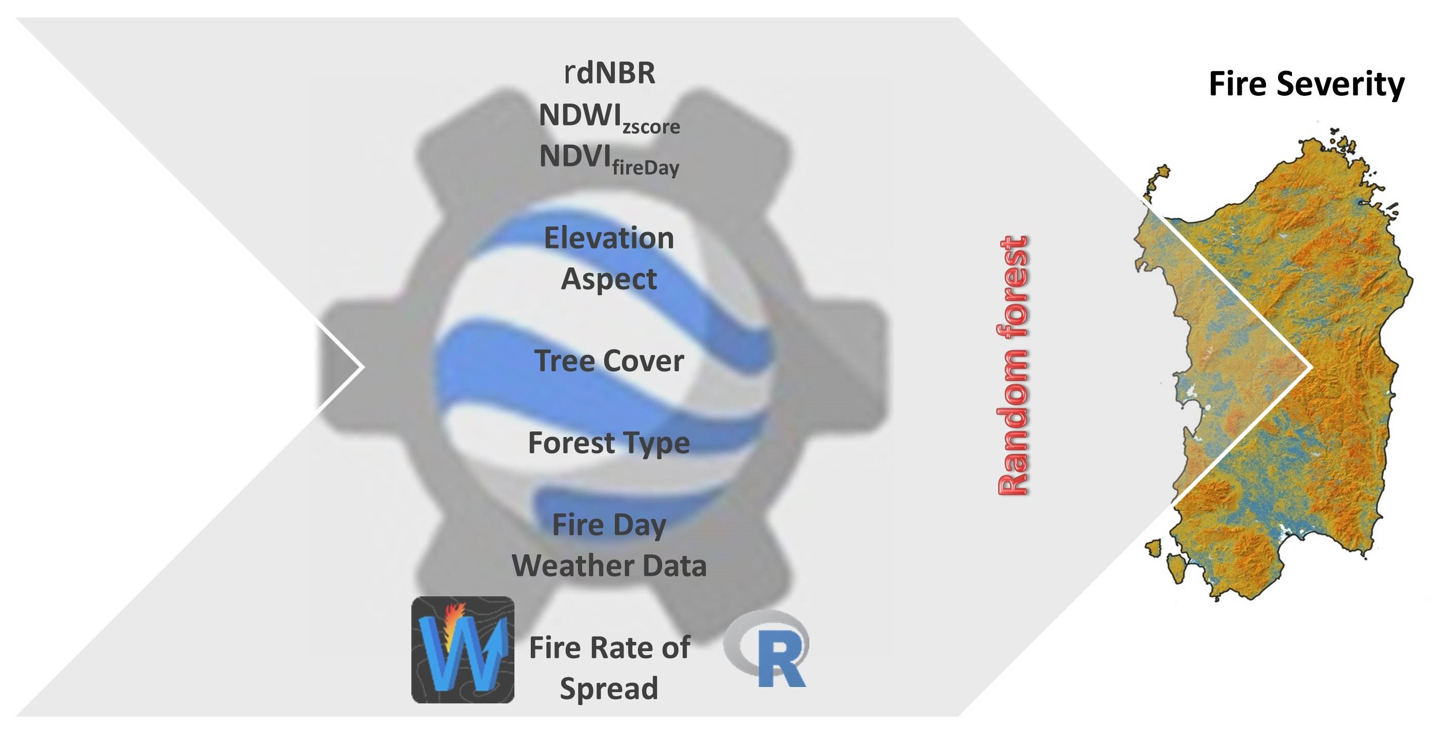
2.4. Explanatory Variables
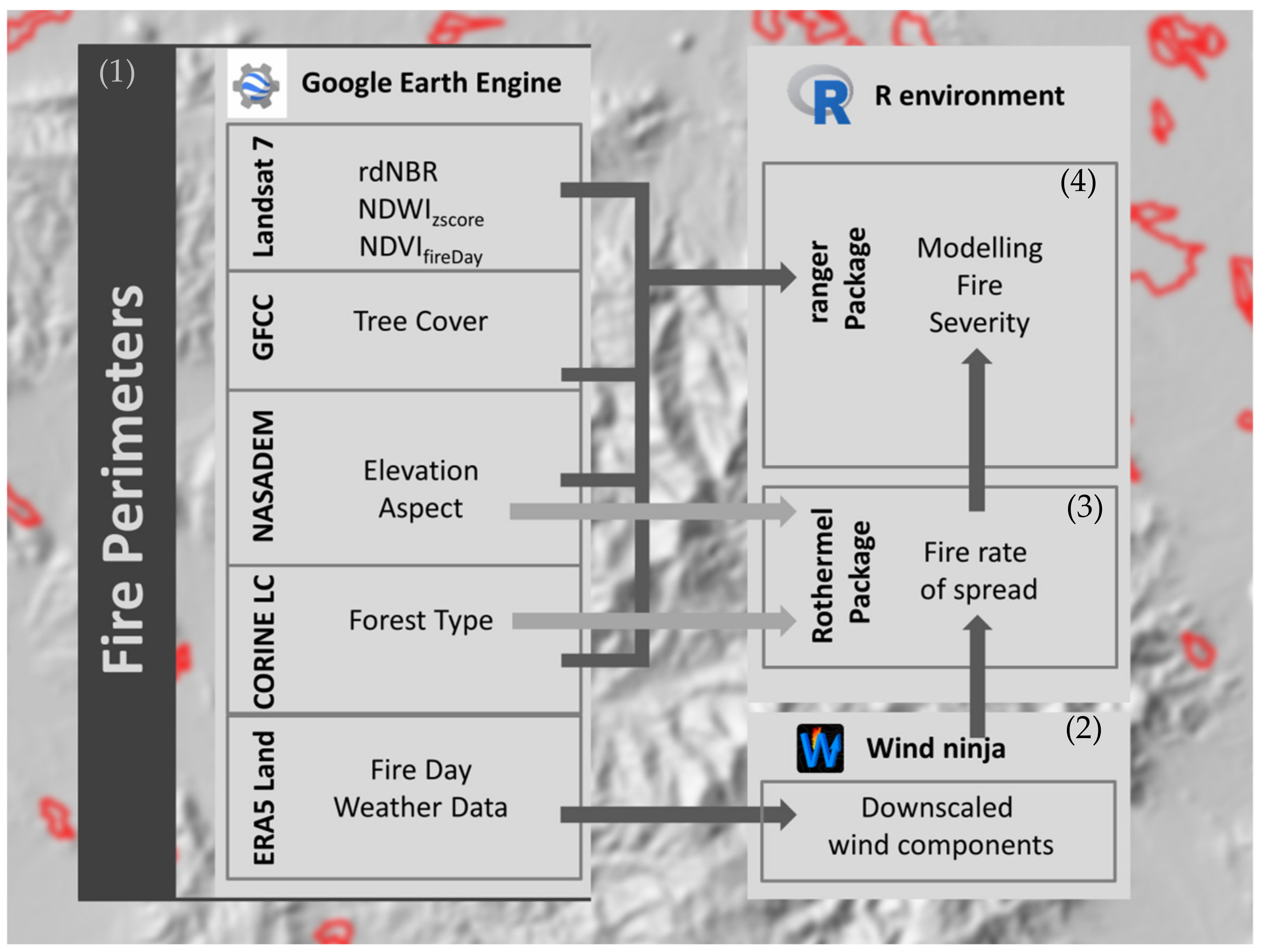
Different types of explanatory variables were initially selected according to previous studies focusing on single fire events [25,32,33]. These variables are included in three broad groups: topography, vegetation, and burning conditions (Figure 3). All datasets were resampled to the rdNBR grid using the scale command in GEE, which uses the nearest neighborhood method by default.
Topographical conditions, i.e., orthometric altitude and aspect (the orientation in relation to geographic North in sexagesimal degrees), were obtained and processed in GEE using the NASADEM dataset at 30-m resolution (https://developers.google.com/earth-engine/datasets/catalog/NASA_NASADEM_HGT_001, accessed on 15 December 2021), which is an improved version of the Shuttle Radar Topography Mission (SRTM).
For defining the vegetation types, we used data from the CORINE Land Cover (CLC) storage on GEE (https://developers.google.com/earth-engine/datasets/catalog/COPERNICUS_CORINE_V20_100m, accessed on 15 December 2021). CLC have 100-m resolution, with 25 ha as the minimum mapping unit (100 m as minimum mapping width) and an accuracy of 25 m. Since CLC data are updated every six years (from 2000 to 2018), the closest previous CLC update to each specific fire event was associated to best represent the vegetation during the fire. For instance, for a fire occurring in 2009, we assigned the CLC 2006 data. This approach assumes that no forest change occurred between the year of the CLC inventory and the fire event. Since we were mainly interested in assessing fire severity on (quasi-) natural ecosystems, only pixels classified by the CLC as (quasi-) natural vegetation areas were used in the analysis (i.e., agro-forestry areas, broad-leaved forests, coniferous forests, agriculture with natural vegetation, mixed forests, pastures, sclerophyllous vegetation, sparsely vegetated areas, and transitional woodland–shrub (i.e., categories at the CLC n3 level)).
Furthermore, vegetation amount was considered in two different ways. For one side, we used the Landsat Vegetation Continuous Fields (https://developers.google.com/earth-engine/datasets/catalog/NASA_MEASURES_GFCC_TC_v3?hl=en, accessed on 15 December 2021), which provides data on tree cover percentage at a resolution of 30 m for the years 2000, 2005, 2010, and 2015. As for CLC data, the closest dataset to each fire date was assigned. On the other side, using the Landsat7 data, we also calculate the Normalized Difference Vegetation Index (NDVI) as a proxy for the total vegetation amount for each specific pixel and date (NDVIfireday). To avoid missing values and to automatize the procedure, we calculate the mean value of NDVI for the two previous scenes.
The effect of vegetation water stress on fire severity was also considered by calculating the Normalized Difference Water Index (NDWI). NDWI uses surface reflectance in the near and shortwave infrared as a proxy of water content [34]. Indeed, several studies showed its great performance in estimating live fuel moisture [35,36]. To make different pixels comparable and, thus, meaningful for model calibration, we followed the standardized (z-) score approach recently proposed by Swetnam et al., [37] using GEE. The approach first calculates the NDWI for the fire day (here, the mean of the previous 30 days, i.e., NDWIday), the mean (NDWImeanRef), and the standard deviation (NDWIsdRef) for a reference period (here the previous 5 years). Then, for NDWIday, we subtract the NDWImeanRef and divide by NDWIsdRef to obtain, as in inferential statistics, a standard score (NDWIzscore) representing the degree of fuel moisture (the lower the value, the greater the dryness). Indeed, this approach proved useful for monitoring ecosystem disturbances [37].
Finally, to account for burning conditions’ effects on fire severity, we calculated the fire rate of spread (ROS) using the function implemented on the R package Rothermel [38]. Indeed, the most commonly used fire spread simulators (e.g., Behave, Flammap, Farsite, and Wildfire Analyst) are based on the Rothermel equation. The Rothermel equation requires data on fuel, topography, and weather conditions during the fire event [39]. CLC classes were reclassified into fuel models following Lozano et al. [7], and topographical conditions were extracted from the NASADEM (see previous paragraphs). We used ERA 5 Land data from GEE (https://developers.google.com/earth-engine/datasets/catalog/ECMWF_ERA5_LAND_HOURLY, accessed on 15 December 2021) to estimate wind direction and speed during each fire day. Since ERA5 Land provides data at 11-km resolution, these data were downscaled to rdNBR resolution (30 m) using the Command Line Interface of WindNinja. WindNinja is a program developed by the American Forest Service that computes spatially varying wind fields in complex terrains [40]. Furthermore, to account for the positive and negative effects of slope and wind alignment on ROS estimation, the wind speed was multiplied by the cosine of the difference between aspect and wind direction (both in degrees).

2.5. Analysis

The random forest algorithm implemented under the R package “ranger” [41] was used to assess the potential predictability of fire severity (i.e., rdNBR) based on the explanatory variables mentioned in the previous section. Random forest is a well-recognized and commonly used machine learning algorithm based on classification trees [42]. Random forest is a nonparametric algorithm which fits several trees by randomly splitting the original sample at each iteration. The two parameters required to generate the model are the number of classification trees and the number of variables available for splitting each node. These parameters were set as default values, i.e., 500 trees and the square root of the number of variables. Following previous studies, the model’s predictive power was assessed with the internal splitting of the dataset when building each decision tree (e.g., [33]). The random forest algorithm uses two thirds of the data for training and the remaining third for validation (called out-of-bag samples, OOB). OOB samples represent the validation set and are used only in the decision trees that do not include them in the training step. The final prediction is the average among all decision trees predicting each OOB sample. Thus, these OOB samples are used to validate the model by estimating the variance explained by the model and the mean absolute error [42].
Furthermore, we also assessed the model’s classification accuracy by calculating the area under the receiver operating characteristics curve (AUC), a common metric used when assessing accuracy with classification algorithms [43]. Moreover, in this case, two thirds of the data were used for training and the remaining third for validation purposes. rdNBR values were classified into low, medium, and high severity categories following the thresholds defined by Parks et al. [27] (<248, 248–544, >544). We acknowledge that thresholds might differ across different regions and, thus, a potential mismatch might lead to wrong interpretations. Nevertheless, since it was an illustrative example, and we strictly followed the procedure suggested by Parks et al. [27], we consider it more adequate to use those values. Furthermore, some studies using rdNBR in Mediterranean environments observed and used similar values (e.g., [24], <310, 310–640, >640).
We assessed the importance of each variable in the model using the variance impurity as implemented in the “ranger” package [41]. In addition, to interpret the effect of the explanatory variables, we used partial dependence plots (pdp) as implemented on the R package “pdp” [44]. Pdp are commonly used to interpret the outputs of black-box models representing the explanatory variables’ marginal effect (yhat) on the response.
Finally, the model was projected for a specific area of interest to show how the approach could be dynamically implemented for operational purposes. We accounted for the environmental conditions of one specific random date (note that the model can be projected over time to account for varying factors as NDWIzscore, here used as a proxy of fuel moisture content). Sardinia was selected for this exercise, since a significant percentage of fire records used for calibration belong to this region, and thus results are expected to be more robust.

3. Results

rdNBR values in the study area ranged from −1132 to 821, with a mean value of 134 (dimensionless, Figure 4). Regarding the explanatory capacity of the rdNBR model, it explained 77% of the variance, with an absolute mean error of 141. The variance explained was similar when calibrating and validating the model separately for each specific forest type (data not shown). When using RF for classifying fire severity into different classes, the general AUC was 0.8 (Figure 5).
The most important variables were tree cover and elevation, followed by the spectral indices NDVIfireday and NDWIzscore (Figure 6).
Regarding the explanatory meaning of the independent variables, rdNBR increased with tree cover, NDVIfireday, and ROS, while decreasing with NDWIzscore and aspect (Figure 7). rdNRB was higher in low and high altitudes but was low under mid altitude locations (i.e., >500 and 1000 m). Across vegetation types, higher values were observed over transitional wood–shrub lands and sclerophyllous shrublands.
As an example, for operational purposes, the model was projected over the island of Sardinia for the 19 August 2019 (Figure 8). The map shows higher potential fire severity along the eastern mountainous areas.

4. Discussion

Building and projecting robust models of fire severity to integrate into risk analysis is of utmost importance for the best decision making. Our modeling exercise showed that robust projections are possible through integrating a considerable number of historical fire records, machine learning algorithms, and online data processing platforms. Indeed, GEE emerged as an excellent resource for data acquisition and manipulation in wildfire management. It allowed for online processing of topographical, climatological, land use, and spectral variables, saving time and computational resources. Indeed, previous studies already showed the potential benefits of using GEE across different topics within the wildfire risk management field, e.g., fuel moisture, fire severity proxies, or recovery trajectories [35,45,46]. Furthermore, the procedure suggested by Parks et al. [27] to estimate rdNBR under GEE allowed consideration of a great number of fires leading to robust model calibration. Beyond being much faster since no curated scene selection is required, this procedure was also shown to be potentially more accurate when estimating field metrics of fire severity, such as the composite burn index [27].
rdNBR values in the study area were mainly within the range of observed data in other Euro-Mediterranean countries, such as France, Spain, Portugal, or Greece [22,25]. However, in our results, we observed a greater proportion of negative values (i.e., without severity), most likely since we used fire perimeters with no information on inner unburned areas. On the other hand, based on single fire events, previous studies focused on sampled locations (and, thus, had a more accurate delineation of burnt areas).
The model’s performance when estimating rdNBR was within the range, even greater, of previous studies focused on single fire events [24,32,33]. Correlation values around 0.75 suggest high confidence for reliable projections. Furthermore, the performance of our models did not differ across forest types, suggesting no potential limitations, at least in Mediterranean areas for which wildfires are a major threat. Comparing with previous studies, the advantage of our approach is that the explanatory capacity of the model relies on readily available data. That is, our approach does not need variables that are not easy to find, such as those derived from Lidar data. Indeed, despite the high potential of previous studies for guiding local-scale management actions (e.g., fuel treatments), they might find difficulties for risk analysis over large areas, especially where Lidar data are unavailable.
Our model performance was also highly satisfactory when using severity classes, showing a good capacity to discriminate different degrees of fire severity. Our exercise was based on the categories suggested by Parks et al. [27]. Still, they can be adapted with little effort to different thresholds defined by using field data or suggested in other studies (ensuring that rdNBR estimations follow a similar procedure). In addition, when uncertainties arise when defining thresholds to differentiate severity classes, it is possible to use varying values and, thus, obtain projected severity classes in a probability manner. The strong results that we obtained, based on large fire databases over large areas, suggest a great potential for consideration in risk analysis/mapping in an operational way.
Our study’s most important drivers of fire severity were tree cover, elevation, and the spectral indices representing fuel amount and dryness, i.e., NDVIfireday and NDWIzscore, respectively. Our results showed that fire severity is higher when tree cover and total live fuel amount increase (NDVIfireday). Indeed, previous studies also noticed the great importance of vegetation amount on fire severity by using different proxies [24,32,33]. A greater amount of vegetation biomass might lead to greater fire intensity, which ultimately translates into greater impacts on vegetation/ecosystem [1,47]. Indeed, it was shown that biomass, across large scales, is a limiting factor in fire severity [30]. Interestingly, elevation emerged as an important variable in explaining fire severity. Although many studies did not consider elevation for modeling purposes, Mitsopoulos et al. [22] also identified it as the most important topographical variable. It was suggested that topographical variables somehow represent multiple processes affecting fire behavior. Indeed, when analyzing the pdp plots, they suggest that elevation represents some hidden factors that influence severity, especially at low and high altitudes. For instance, D’este et al. [48] showed that elevation in southern Italy significantly explains the spatial distribution of dead fuels.
Our results also showed the importance of plant water stress on fire severity. Previous studies at a lower scale also observed this effect [33]. It is well known that water stress might affect the completeness of combustion and fuel flammability [49,50], which ultimately translates into higher fire severity. Surprisingly, ROS was the variable with the lowest importance in the model. Its effects on severity were predicted to be greater at high ROS. Previous studies already observed this pattern but with higher importance in the model [32]. It was argued that, according to the Rothermel surface model, fire line intensity directly increases with ROS [51]. Indeed, it was observed that tree mortality is greater in fast-moving fires [52]. It is important to notice that, compared to “in situ observed” variables, such as NDVIfireday and NDWIzscore, ROS comes from a modeling approach that integrates modeled/adjusted variables, such as wind components and fuel types. Thus, the greater uncertainties associated with ROS might potentially influence the observed results.
Overall, it is important to notice that the major or minor role of different variables might be case study sensitive, depending on factors such as the study area, satellite used for severity estimations, or the remote sensing index used. For instance, Viedma et al. [32] showed how the relative importance of different explanatory variables changed when using sentinel 2 and Landsat 8. Furthermore, it was also shown how results changed depending on using different spectral indices (i.e., dNBR, rdNBR, or RBR). Thus, the relative importance of the different variables should be understood with caution, acknowledging the theoretical background.

5. Conclusions

Our results, tested within the Mediterranean region, showed that is feasible to obtain reliable projections of potential fire severity using historical fire records, remote sensing data, and machine learning algorithms. Our approach could be easily implemented across different areas and only requires historical fire perimeters, proving beneficial to anticipate decisions for risk management. Furthermore, the approach presented allows the limitations of previous studies to be overcome, i.e., based on few fire events, allowing for spatial projections and large-scale generalizations.

Author Contributions

Conceptualization, J.M.C.-S.; methodology, J.M.C.-S.; formal analysis J.M.C.-S.; resources, J.M.C.-S., V.B., C.R. and A.M.; data curation, J.M.C.-S. and C.R.; writing—original draft preparation, J.M.C.-S.; writing—review and editing, J.M.C.-S., V.B., C.R., D.S., A.M. and C.S.; project administration, C.S.; funding acquisition, C.S., V.B. and D.S. All authors have read and agreed to the published version of the manuscript.

Funding

This research received no external funding.

Acknowledgments

This work was developed under the framework of the MEDSTAR project funded by the Italy–France Maritime Cross-border Cooperation Program INTERREG 2014–2020.

Conflicts of Interest

The authors declare no conflict of interest.

References

  1. He, T.; Lamont, B.B.; Pausas, J.G. Fire as a key driver of Earth’s biodiversity. Biol. Rev. 2019, 94, 1983–2010. [Google Scholar] [CrossRef]
  2. Pausas, J.G.; Llovet, J.; Rodrigo, A.; Vallejo, V.R. Are wildfires a disaster in the Mediterranean basin?—A review. Int. J. Wildl. Fire 2008, 17, 713–723. [Google Scholar] [CrossRef]
  3. Ruffault, J.; Curt, T.; Martin-Stpaul, N.K.; Moron, V.; Trigo, R.M. Extreme wildfire events are linked to global-change-type droughts in the northern Mediterranean. Nat. Hazards Earth Syst. Sci. 2018, 18, 847–856. [Google Scholar] [CrossRef]
  4. Rodrigues, M.; Jiménez-Ruano, A.; de la Riva, J. Fire regime dynamics in mainland Spain. Part 1: Drivers of change. Sci. Total Environ. 2020, 721, 135841. [Google Scholar] [CrossRef]
  5. Masson-Delmotte, V.; Zhai, P.; Pirani, A.; Connors, S.L.; Péan, C.; Berger, S.; Caud, N.; Chen, Y.; Goldfarb, L.; Gomis, M.I.; et al. Climate Change 2021: The Physical Science Basis. Contribution of Working Group I to the Sixth Assessment Report of the Intergovernmental Panel on Climate Change; Cambridge University Press: Cambridge, UK; New York, NY, USA, 2021. [Google Scholar]
  6. Pausas, J.; Vallejo, R. The role of fire in European Mediterranean Ecosystems. In Remote Sensing of Large Wildfires; Springer: Berlin/Heidelberg, Germany, 1999; pp. 3–16. [Google Scholar] [CrossRef]
  7. Lozano, O.M.; Salis, M.; Ager, A.A.; Arca, B.; Alcasena, F.J.; Monteiro, A.T.; Finney, M.A.; Del Giudice, L.; Scoccimarro, E.; Spano, D. Assessing Climate Change Impacts on Wildfire Exposure in Mediterranean Areas. Risk Anal. 2017, 37, 1898–1916. [Google Scholar] [CrossRef] [PubMed]
  8. Salis, M.; Ager, A.A.; Alcasena, F.J.; Arca, B.; Finney, M.A.; Pellizzaro, G.; Spano, D. Analyzing seasonal patterns of wildfire exposure factors in Sardinia, Italy. Environ. Monit. Assess. 2015, 187, 4175. [Google Scholar] [CrossRef]
  9. Elia, M.; D’Este, M.; Ascoli, D.; Giannico, V.; Spano, G.; Ganga, A.; Colangelo, G.; Lafortezza, R.; Sanesi, G. Estimating the probability of wildfire occurrence in Mediterranean landscapes using Artificial Neural Networks. Environ. Impact Assess. Rev. 2020, 85, 106474. [Google Scholar] [CrossRef]
  10. Leuenberger, M.; Parente, J.; Tonini, M.; Pereira, M.G.; Kanevski, M. Wildfire susceptibility mapping: Deterministic vs. stochastic approaches. Environ. Model. Softw. 2018, 101, 194–203. [Google Scholar] [CrossRef]
  11. Bedia, J.; Golding, N.; Casanueva, A.; Iturbide, M.; Buontempo, C.; Gutierrez, J.M. Seasonal predictions of Fire Weather Index: Paving the way for their operational applicability in Mediterranean Europe. Clim. Serv. 2018, 9, 101–110. [Google Scholar] [CrossRef]
  12. Vitolo, C.; Di Giuseppe, F.; Barnard, C.; Coughlan, R.; San-Miguel-Ayanz, J.; Libertá, G.; Krzeminski, B. ERA5-based global meteorological wildfire danger maps. Sci. Data 2020, 7, 216. [Google Scholar] [CrossRef]
  13. Gignoux, J.; Clobert, J.; Menaut, J.C. Alternative fire resistance strategies in savanna trees. Oecologia 1997, 110, 576–583. [Google Scholar] [CrossRef] [PubMed]
  14. Fernandes, P.M.; Vega, J.A.; Jiménez, E.; Rigolot, E. Fire resistance of European pines. For. Ecol. Manag. 2008, 256, 246–255. [Google Scholar] [CrossRef]
  15. Sugihara, N.; van Wagtendonk, J.; Fites-Kaufman, J. Fire as an ecological process. In Fire California’s Ecosystems; University of California Press: Berkeley, CA, USA, 2006; pp. 58–74. [Google Scholar] [CrossRef]
  16. Keeley, J.E. Fire intensity, fire severity and burn severity: A brief review and suggested usage. Int. J. Wildl. Fire 2009, 18, 116–126. [Google Scholar] [CrossRef]
  17. Key, C.H.; Benson, N.C. Landscape Assessment (LA) Sampling and Analysis Methods; General Technical Report RMRS-GTR; USDA Forest Service: Ogden, UT, USA, 2006.
  18. de Santis, A.; Chuvieco, E. GeoCBI: A modified version of the Composite Burn Index for the initial assessment of the short-term burn severity from remotely sensed data. Remote Sens. Environ. 2009, 113, 554–562. [Google Scholar] [CrossRef]
  19. Miller, J.D.; Thode, A.E. Quantifying burn severity in a heterogeneous landscape with a relative version of the delta Normalized Burn Ratio (dNBR). Remote Sens. Environ. 2007, 109, 66–80. [Google Scholar] [CrossRef]
  20. Cocke, A.E.; Fulé, P.Z.; Crouse, J.E. Comparison of burn severity assessments using Differenced Normalized Burn Ratio and ground data. Int. J. Wildl. Fire 2005, 14, 189–198. [Google Scholar] [CrossRef]
  21. Miller, J.D.; Knapp, E.E.; Key, C.H.; Skinner, C.N.; Isbell, C.J.; Creasy, R.M.; Sherlock, J.W. Calibration and validation of the relative differenced Normalized Burn Ratio (RdNBR) to three measures of fire severity in the Sierra Nevada and Klamath Mountains, California, USA. Remote Sens. Environ. 2009, 113, 645–656. [Google Scholar] [CrossRef]
  22. Cardil, A.; Mola-Yudego, B.; Blázquez-Casado, Á.; González-Olabarria, J.R. Fire and burn severity assessment: Calibration of Relative Differenced Normalized Burn Ratio (RdNBR) with field data. J. Environ. Manag. 2019, 235, 342–349. [Google Scholar] [CrossRef]
  23. Soverel, N.O.; Perrakis, D.D.B.; Coops, N.C. Estimating burn severity from Landsat dNBR and RdNBR indices across western Canada. Remote Sens. Environ. 2010, 114, 1896–1909. [Google Scholar] [CrossRef]
  24. Viedma, O.; Quesada, J.; Torres, I.; de Santis, A.; Moreno, J.M. Fire Severity in a Large Fire in a Pinus pinaster Forest is Highly Predictable from Burning Conditions. Stand Structure, and Topography. Ecosystems 2015, 18, 237–250. [Google Scholar] [CrossRef]
  25. Mitsopoulos, I.; Chrysafi, I.; Bountis, D.; Mallinis, G. Assessment of factors driving high fire severity potential and classification in a Mediterranean pine ecosystem. J. Environ. Manag. 2019, 235, 266–275. [Google Scholar] [CrossRef] [PubMed]
  26. Araujo, M.B.; Peterson, A.T. Uses and misuses of bioclimatic envelope modelling. Ecology 2012, 93, 1527–1539. [Google Scholar] [CrossRef]
  27. Parks, S.A.; Holsinger, L.M.; Voss, M.A.; Loehman, R.A.; Robinson, N.P. Mean composite fire severity metrics computed with google earth engine offer improved accuracy and expanded mapping potential. Remote Sens. 2018, 10, 879. [Google Scholar] [CrossRef]
  28. Guidon, L. Trends in wildfire burn severity across Canada, 1985 to 2015. Can. J. For. Res. 2020, 51, 1230–1244. [Google Scholar] [CrossRef]
  29. García-Llamas, P.; Suárez-Seoane, S.; Fernández-Guisuraga, J.M.; Fernández-García, V.; Fernández-Manso, A.; Quintano, C.; Taboada, A.; Marcos, E.; Calvo, L. Evaluation and comparison of Landsat 8, Sentinel-2 and Deimos-1 remote sensing indices for assessing burn severity in Mediterranean fire-prone ecosystems. Int. J. Appl. Earth Obs. Geoinf. 2019, 80, 137–144. [Google Scholar] [CrossRef]
  30. Parks, S.A.; Parisien, M.A.; Miller, C.; Dobrowski, S.Z. Fire activity and severity in the western US vary along proxy gradients representing fuel amount and fuel moisture. PLoS ONE 2014, 9, e99699. [Google Scholar] [CrossRef]
  31. Foga, S.; Scaramuzza, P.L.; Guo, S.; Zhu, Z.; Dilley, R.D.; Beckmann, T.; Schmidt, G.L.; Dwyer, J.L.; Hughes, M.J.; Laue, B. Cloud detection algorithm comparison and validation for operational Landsat data products. Remote Sens. Environ. 2017, 194, 379–390. [Google Scholar] [CrossRef]
  32. Viedma, O.; Chico, F.; Fernández, J.J.; Madrigal, C.; Safford, H.D.; Moreno, J.M. Disentangling the role of prefire vegetation vs. burning conditions on fire severity in a large forest fire in SE Spain. Remote Sens. Environ. 2020, 247, 111891. [Google Scholar] [CrossRef]
  33. García-Llamas, P.; Suárez-Seoane, S.; Taboada, A.; Fernández-Manso, A.; Quintano, C.; Fernández-García, V.; Fernández-Guisuraga, J.M.; Marcos, E.; Calvo, L. Environmental drivers of fire severity in extreme fire events that affect Mediterranean pine forest ecosystems. For. Ecol. Manag. 2019, 433, 24–32. [Google Scholar] [CrossRef]
  34. Gao, B.C. NDWI—A normalized difference water index for remote sensing of vegetation liquid water from space. Remote Sens. Environ. 1996, 58, 257–266. [Google Scholar] [CrossRef]
  35. Costa-Saura, J.M.; Balaguer-Beser, Á.; Ruiz, L.A.; Pardo-Pascual, J.E.; Soriano-Sancho, J.L. Empirical models for spatio-temporal live fuel moisture content estimation in mixed mediterranean vegetation areas using sentinel-2 indices and meteorological data. Remote Sens. 2021, 13, 3726. [Google Scholar] [CrossRef]
  36. Chuvieco, E.; Riaño, D.; Aguado, I.; Cocero, D. Estimation of fuel moisture content from multitemporal analysis of Landsat Thematic Mapper reflectance data: Applications in fire danger assessment. Int. J. Remote Sens. 2002, 23, 2145–2162. [Google Scholar] [CrossRef]
  37. Swetnam, T.L.; Yool, S.R.; Roy, S.; Falk, D.A. On the use of standardized multi-temporal indices for monitoring disturbance and ecosystem moisture stress across multiple earth observation systems in the google earth engine. Remote Sens. 2021, 13, 1448. [Google Scholar] [CrossRef]
  38. Vacchiano, G.; Ascoli, D. An Implementation of the Rothermel Fire Spread Model in the R Programming Language. Fire Technol. 2015, 51, 523–535. [Google Scholar] [CrossRef]
  39. Rothermel, R.C. A Mathematical Model for Predicting Fire Spread in Wildland Fuels; Research Paper INT-115; U.S. Department of Agriculture, Intermountain Forest and Range Experiment Station: Ogden, UT, USA, 1972; 40p.
  40. Wagenbrenner, N.S.; Forthofer, J.M.; Page, W.G.; Butler, B.W. Development and evaluation of a reynolds-averaged navier-stokes solver in windninja for operational wildland fire applications. Atmosphere 2019, 10, 672. [Google Scholar] [CrossRef]
  41. Wright, M.N.; Ziegler, A. Ranger: A fast implementation of random forests for high dimensional data in C++ and R. J. Stat. Softw. 2017, 77, 1–17. [Google Scholar] [CrossRef]
  42. Breiman, L. Random forests. Mach. Learn. 2001, 45, 5–32. [Google Scholar] [CrossRef]
  43. Fielding, A.; Bell, J. A review of methods for the assessment of prediction errors in conservation presence/absence models. Environ. Conserv. 1997, 24, 38–49. [Google Scholar] [CrossRef]
  44. Greenwell, B.M. pdp: An R package for constructing partial dependence plots. R J. 2017, 9, 421–436. [Google Scholar] [CrossRef]
  45. Viana-Soto, A.; Aguado, I.; Salas, J.; García, M. Identifying post-fire recovery trajectories and driving factors using landsat time series in fire-prone mediterranean pine forests. Remote Sens. 2020, 12, 1499. [Google Scholar] [CrossRef]
  46. Marcos, B.; Gonçalves, J.; Alcaraz-Segura, D.; Cunha, M.; Honrado, J.P. A framework for multi-dimensional assessment of wildfire disturbance severity from remotely sensed ecosystem functioning attributes. Remote Sens. 2021, 13, 780. [Google Scholar] [CrossRef]
  47. Miquelajauregui, Y.; Cumming, S.G.; Gauthier, S. Modelling variable fire severity in boreal forests: Effects of fire intensity and stand structure. PLoS ONE 2016, 11, e0150073. [Google Scholar] [CrossRef]
  48. D’este, M.; Elia, M.; Giannico, V.; Spano, G.; Lafortezza, R.; Sanesi, G. Machine learning techniques for fine dead fuel load estimation using multi-source remote sensing data. Remote Sens. 2021, 13, 1658. [Google Scholar] [CrossRef]
  49. Fares, S.; Bajocco, S.; Salvati, L.; Camarretta, N.; Dupuy, J.L.; Xanthopoulos, G.; Guijarro, M.; Madrigal, J.; Hernando, C.; Corona, P. Characterizing potential wildland fire fuel in live vegetation in the Mediterranean region. Ann. For. Sci. 2017, 74, 1. [Google Scholar] [CrossRef]
  50. Possell, M.; Bell, T. The influence of fuel moisture content on the combustion of Eucalyptus foliage. Int. J. Wildl. Fire 2012, 22, 343–352. [Google Scholar] [CrossRef]
  51. Andrews, P.L. The Rothermel Surface Fire Spread Model and Associated Developments: A Comprehensive Explanation; General Technical Report RMRS-GTR-371; U.S. Department of Agriculture, Forest Service, Rocky Mountain Research Station: Fort Collins, CO, USA, 2018; 121p.
  52. Hantson, S.; Andela, N.; Goulden, M.; Randerson, J.T. Human-ignited fires result in more extreme fire behavior and ecosystem impacts. Nat. Commun. 2022, 13, 2717. [Google Scholar] [CrossRef] [PubMed]
Figure 1. Map of the study area (a), within the Mediterranean Region (b), which covers the French regions of Provence-Alpes-Côte d’Azur (PACA) and Corse, and the Italian regions of Tuscany, Liguria, and Sardinia. Fire perimeters included in the study (period 2004–2017) are shown in orange (source ONF and CFS).
Remotesensing 14 04812 g001
Figure 2. Number of pixels (30-m resolution) under analysis within the studied area (period 2004–2017) across CLC vegetation types (a) and fire frequency (b) across different months and fire size classes (in ha).
Remotesensing 14 04812 g002
Figure 3. Data processing workflow. Fire perimeters are used to extract information in Google Earth Engine, at pixel level, regarding surface reflectance (to calculate the spectral indices), topography within the fire perimeter, vegetation characteristics (type and cover), and wind conditions during each fire event (1). Wind conditions are downscaled to the rdNBR grid using WindNinja (2). These data, together with the corresponding topographical conditions and Corine land cover class, are used to feed the Rothermel package in R to calculate the potential rate of spread for each pixel within each fire perimeter (3). Finally, the random forest algorithm is used to calibrate and validate an empirical fire severity model using the ranger Package in R (4).
Remotesensing 14 04812 g003
Figure 4. Histogram of rdNBR values ((a), calculated using the fire perimeters within the study area during the period 2004–2017; ONF and CFS datasets) and predicted versus observed rdNBR ((b), Pearson correlation coefficient 0.88).
Remotesensing 14 04812 g004
Figure 5. Area under the ROC curve for each severity class (a). Percentage of pixels classified into each severity class (b).
Remotesensing 14 04812 g005
Figure 6. Relative importance of the explanatory variables used for modeling rdNBR. See Section 2 for data sources.
Remotesensing 14 04812 g006
Figure 7. Partial dependence plots showing the marginal effect (yhat) of each explanatory variable (ag) on rdNBR. Vertical black marks represent deciles values of each explanatory variable.
Remotesensing 14 04812 g007
Figure 8. Projected potential fire severity (rdNBR) for the 19 August 2019 in Sardinia (relief data also provided).
Remotesensing 14 04812 g008
Publisher’s Note: MDPI stays neutral with regard to jurisdictional claims in published maps and institutional affiliations.

