
Automated Small River Mapping (ASRM) for the Qinghai-Tibet Plateau Based on Sentinel-2 Satellite Imagery and MERIT DEM

Abstract
:
1. Introduction
2. Materials and Methods
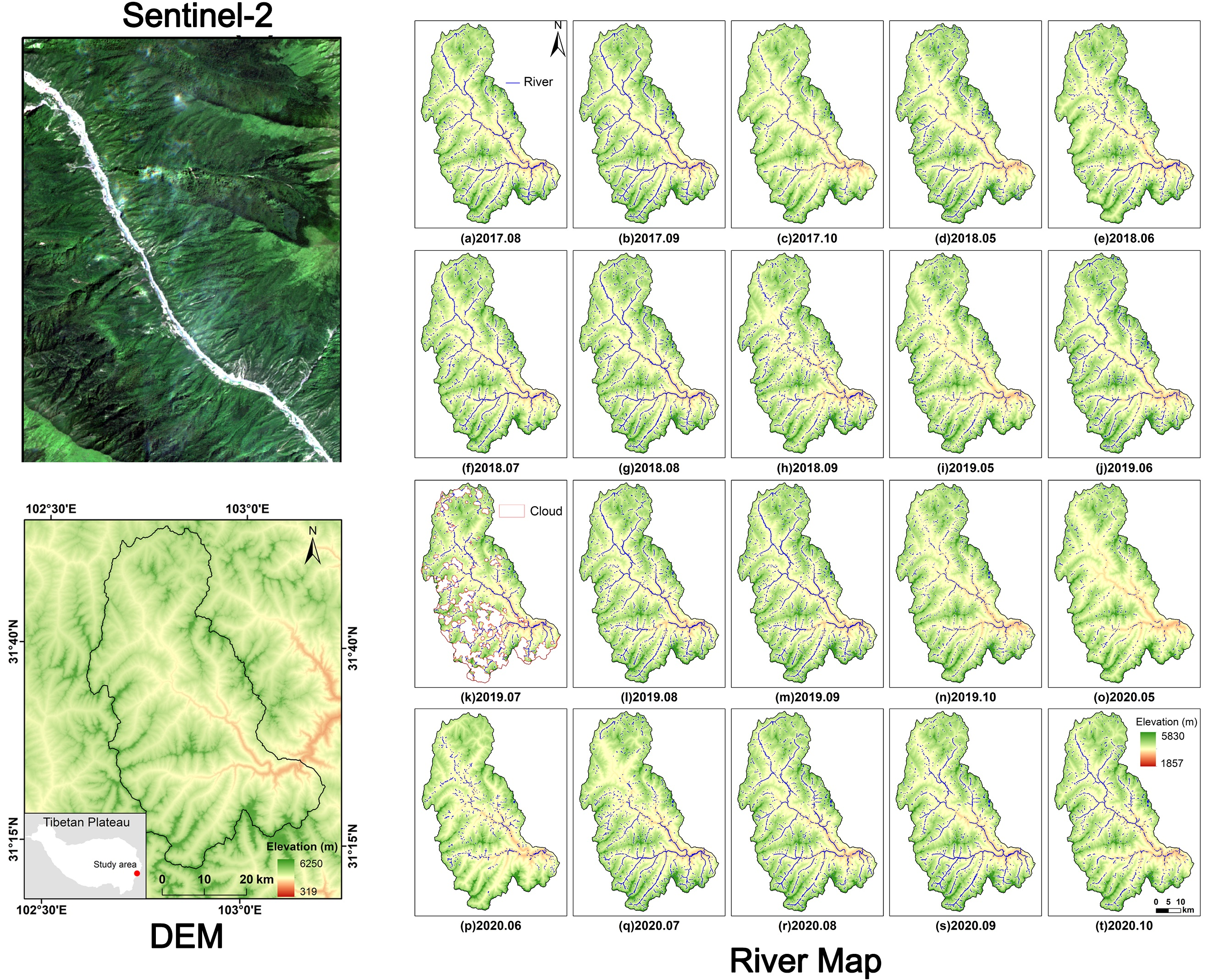
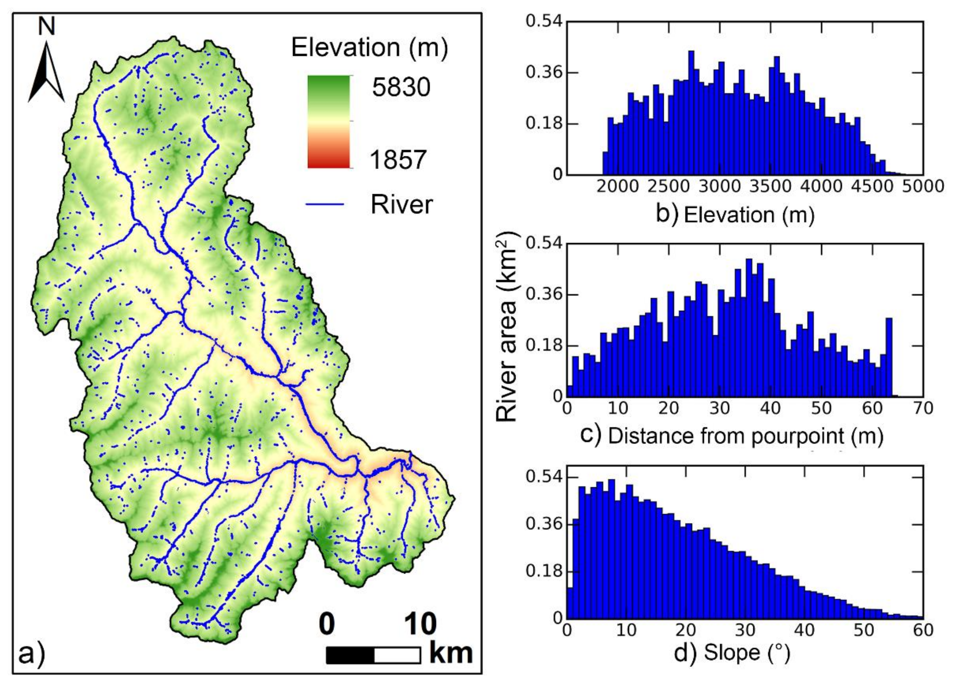
2.1. Study Area
2.2. Data
2.2.1. Satellite Data
2.2.2. Digital Elevation Model (DEM)
2.2.3. Existing Remote Sensing River Network Products
- (1)
- FROM-GLC10: 10-m spatial resolution global land cover product
- (2)
- GSW: Long-time-series remote sensing dataset
- (3)
- GRWL: A global river network dataset with river width
- (4)
- OSM: Real-time update of a global geographic dataset
- (5)
- HydroSHEDS: A global river network dataset produced from DEM
2.2.4. Validation Data
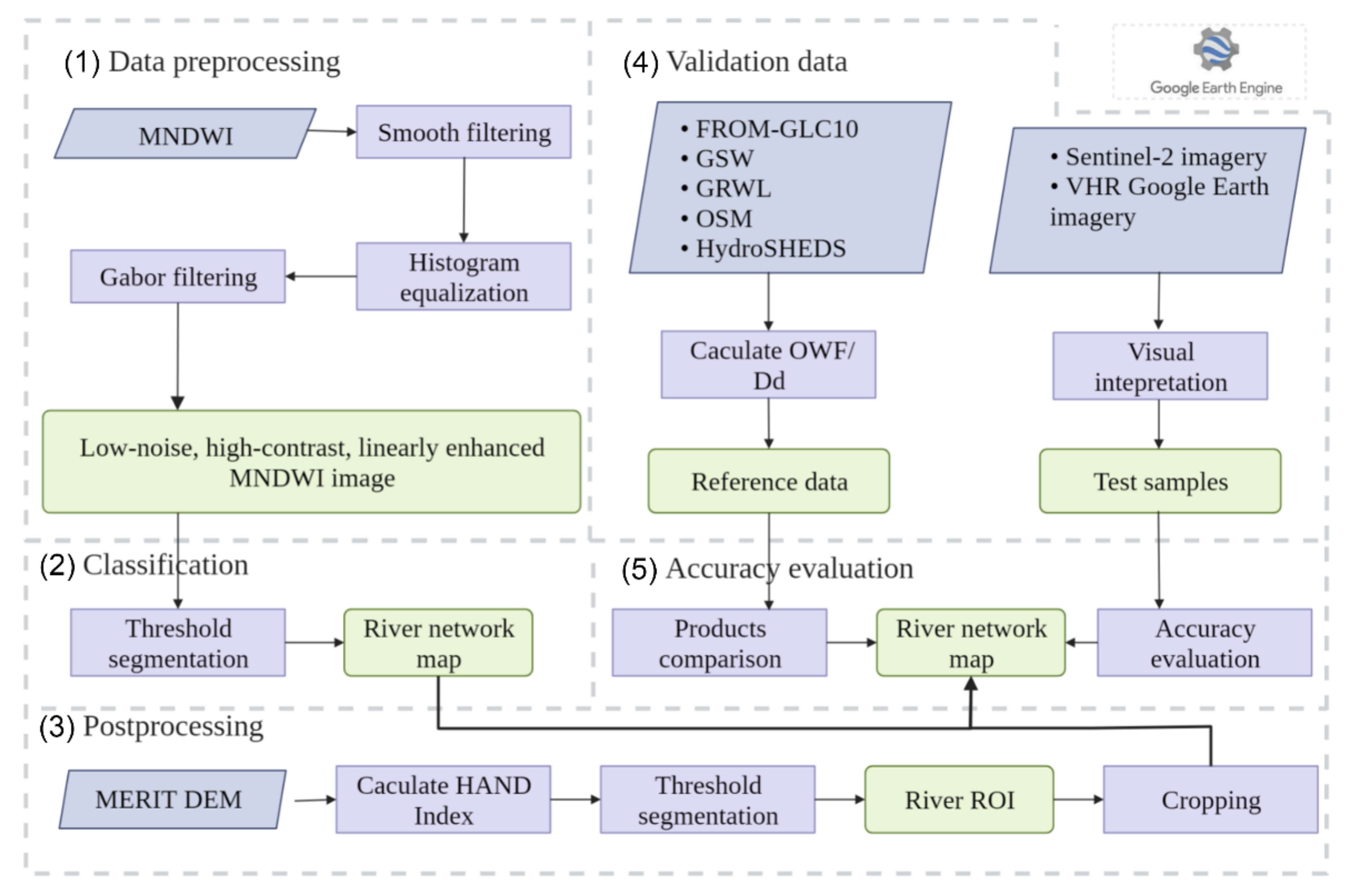
2.3. Automated Small River Mapping
2.3.1. Water Index
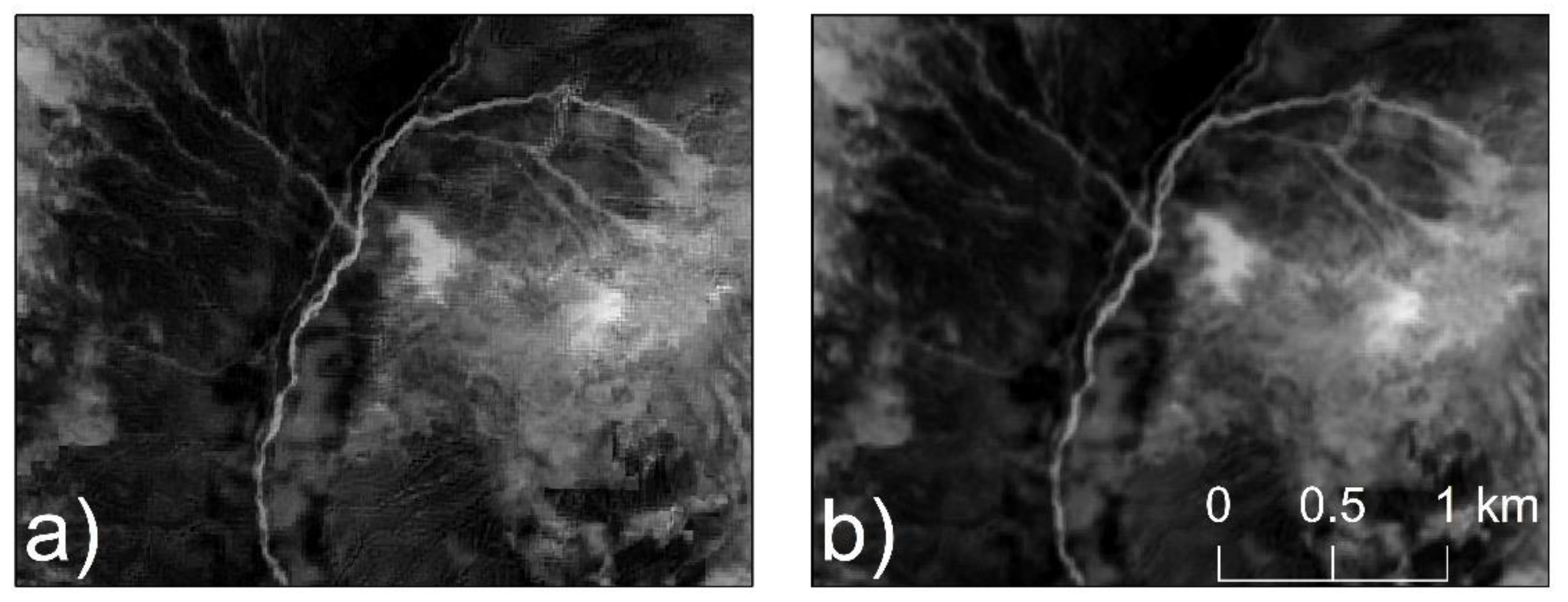
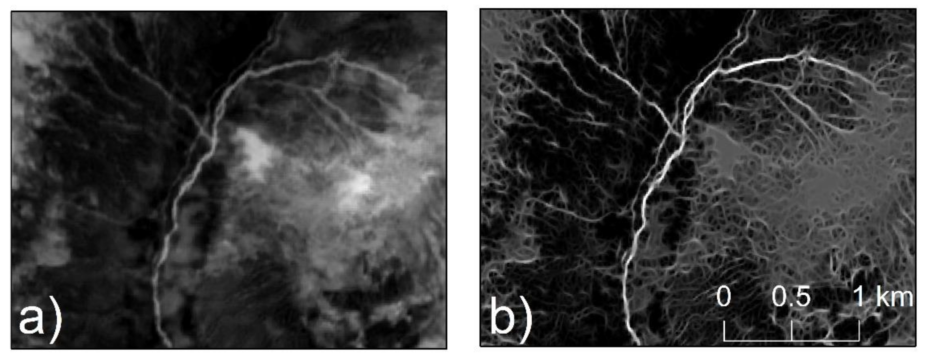
2.3.2. River Enhancement
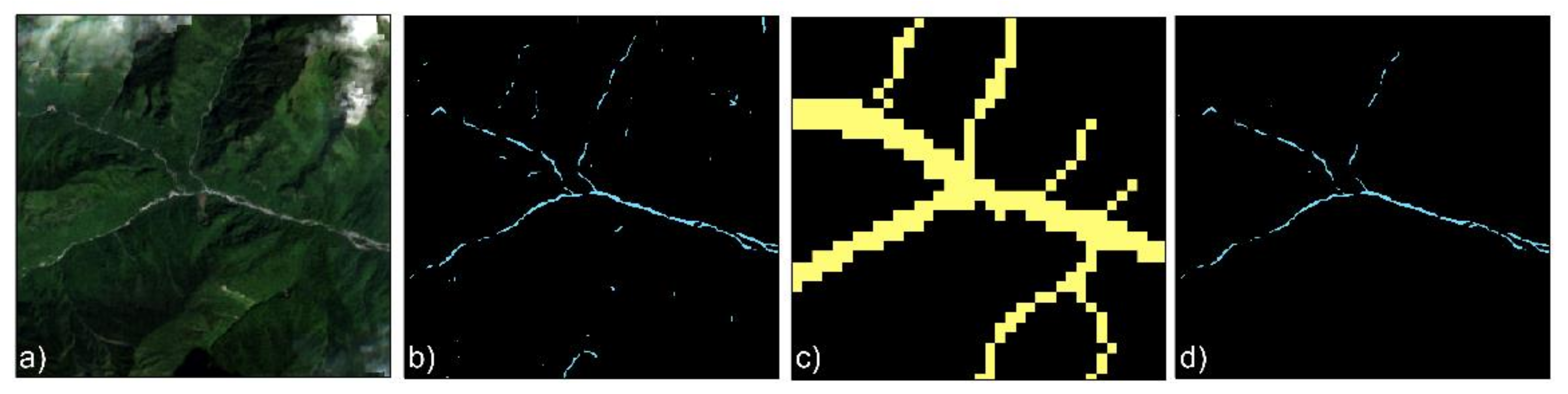
2.3.3. Post-Processing
2.4. Accuracy Evaluation
3. Results
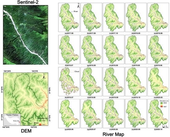
3.1. Results of ASRM
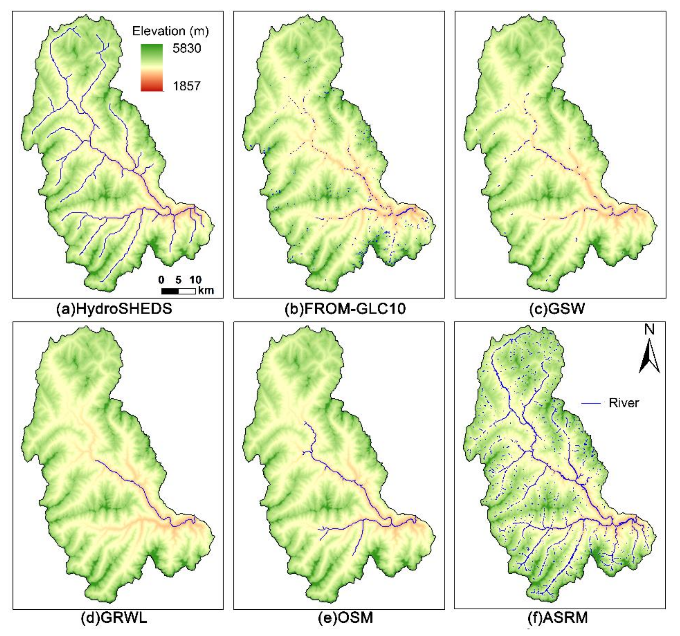
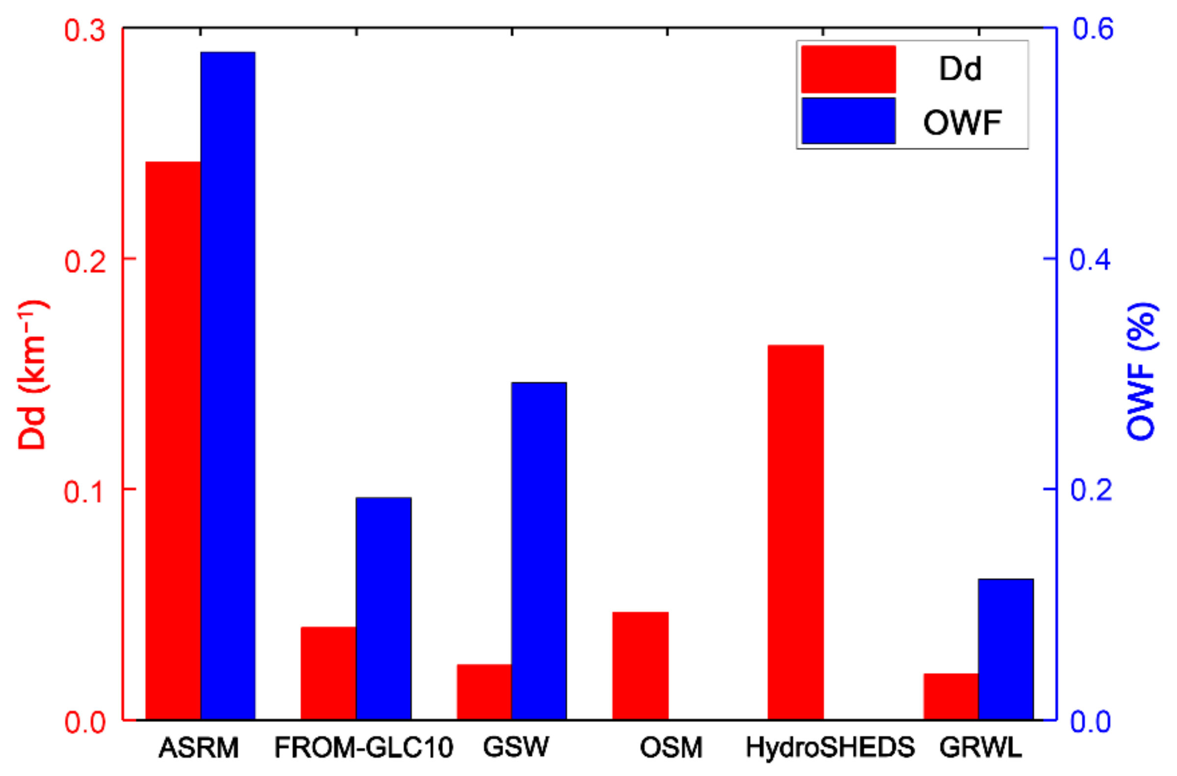
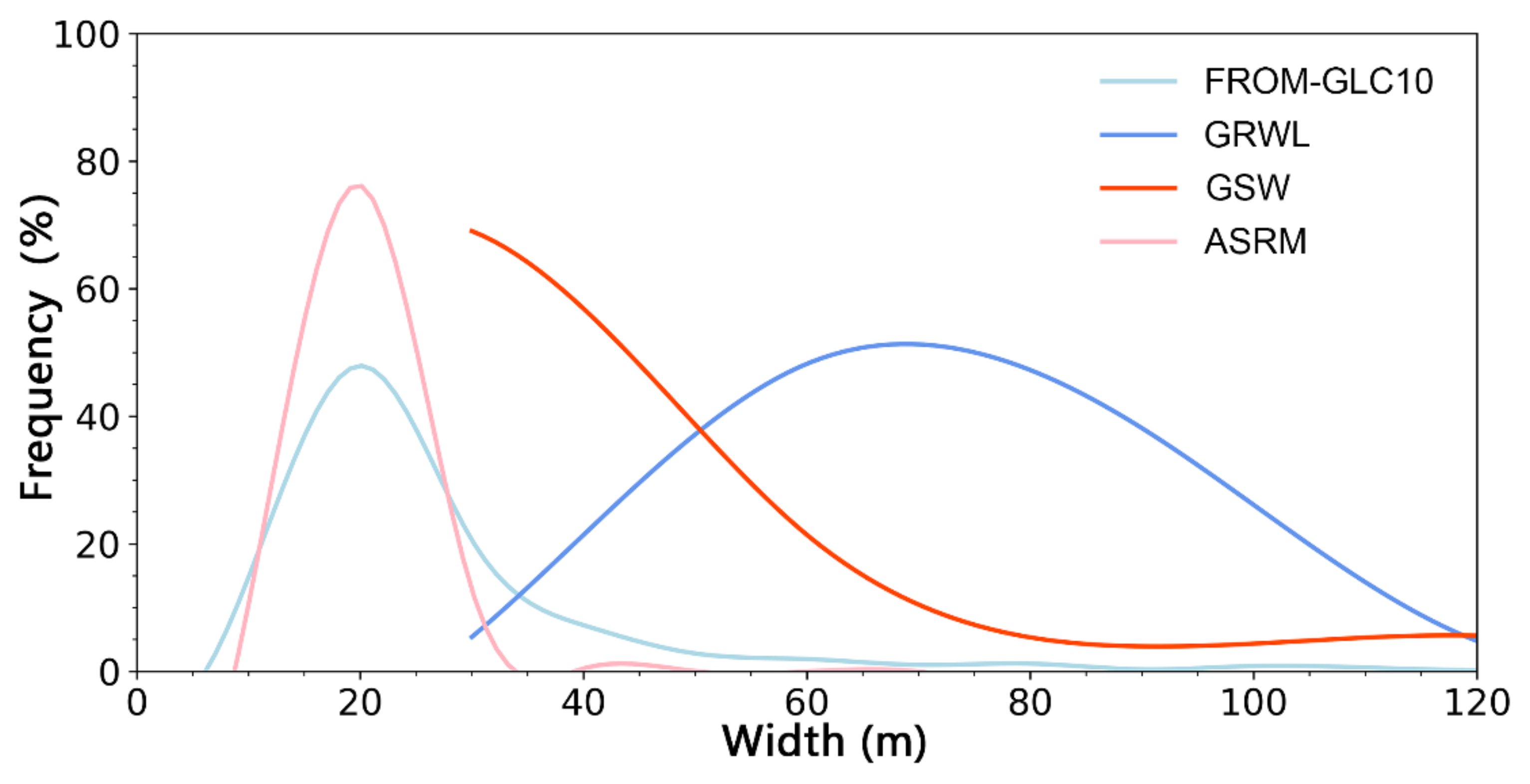
3.2. Assessment against Existing River Network Products
4. Discussion
4.1. Advantages of the Proposed Method over Existing Datasets
4.2. Dynamic Monitoring in Water Surface of the River Networks in the Study Area
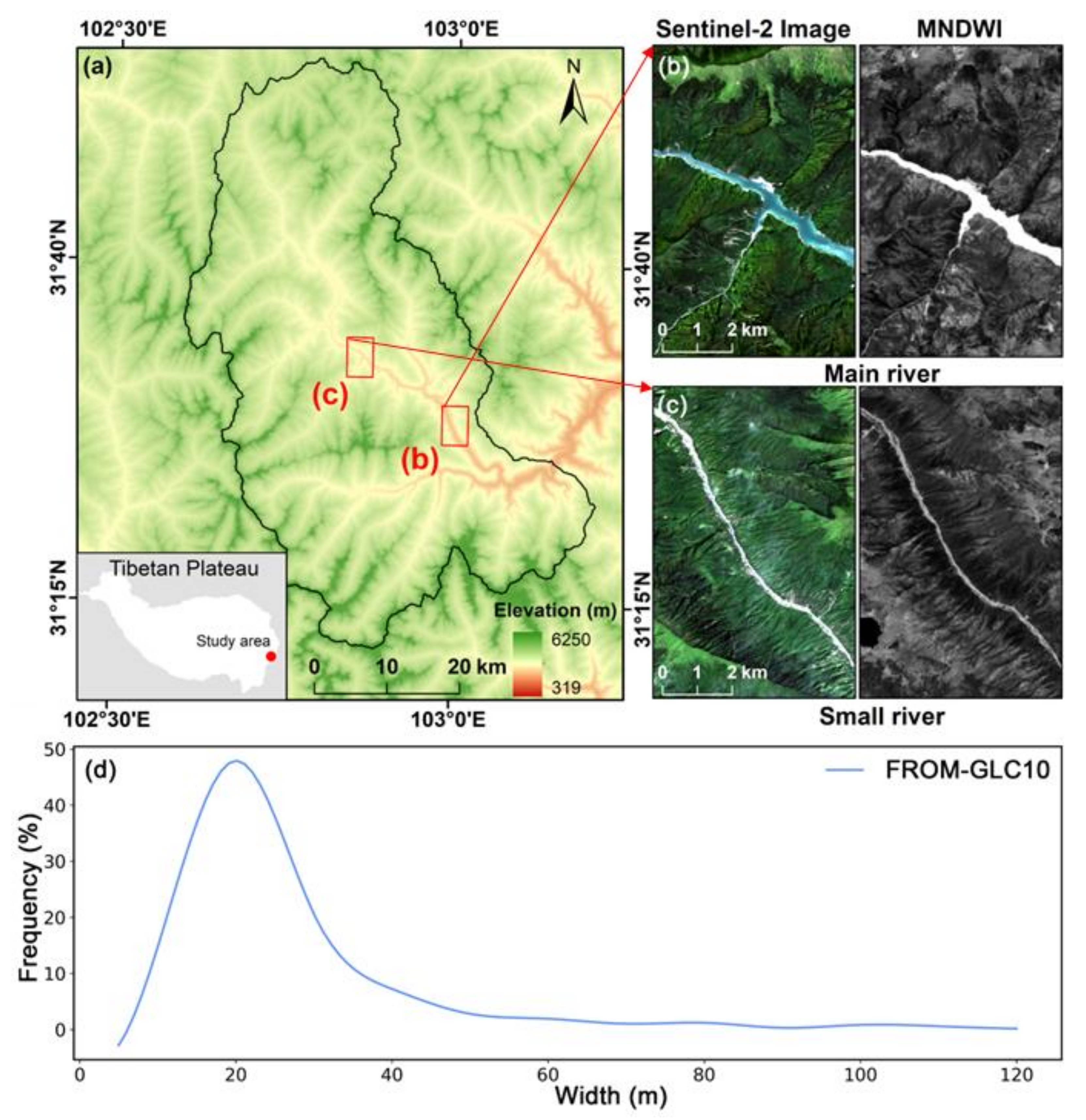
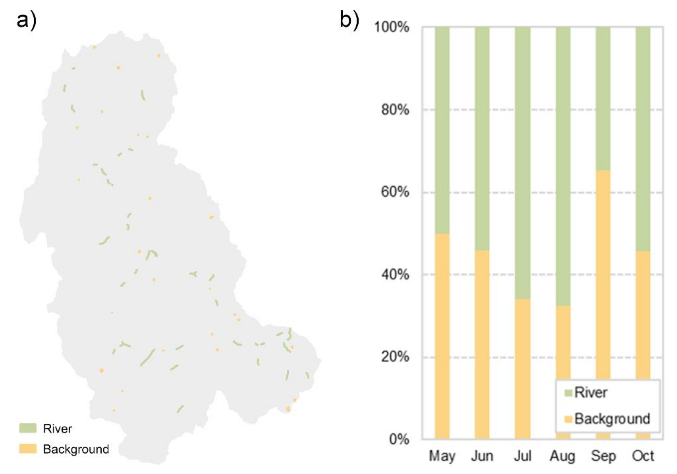
4.2.1. Spatial Distribution Characteristics of the River Networks
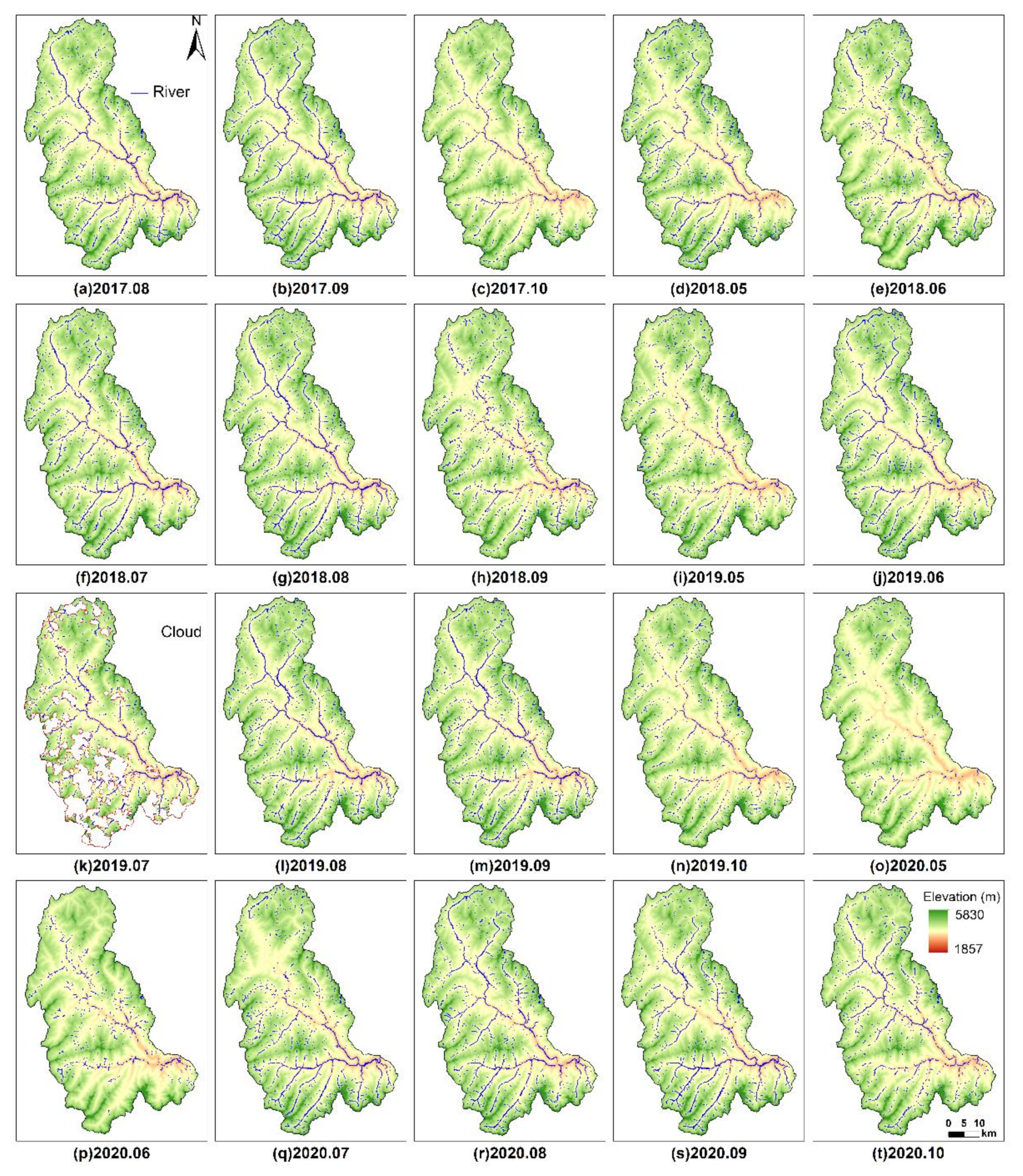
4.2.2. Dynamic Variation in Water Surface of the River Networks
- (1)
- Annual Dynamic Variation
- (2)
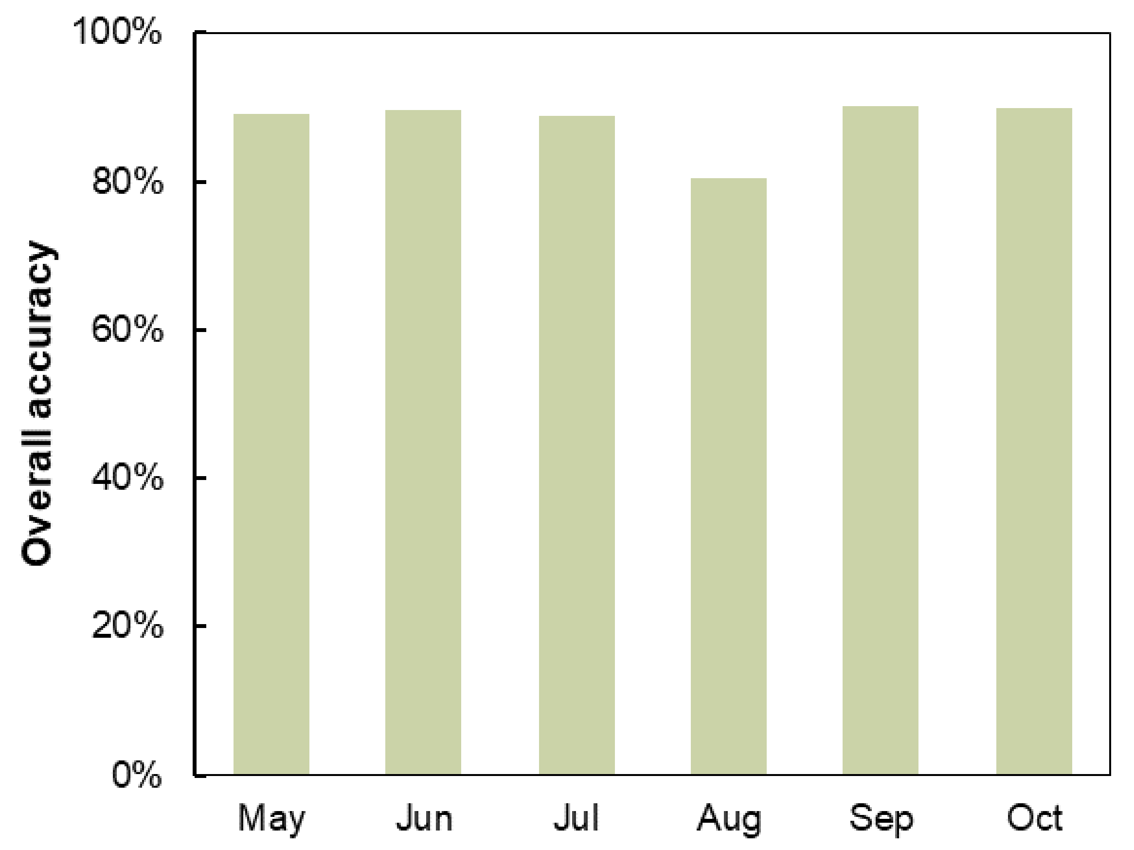
- Seasonal Variation
5. Conclusions
- (1)
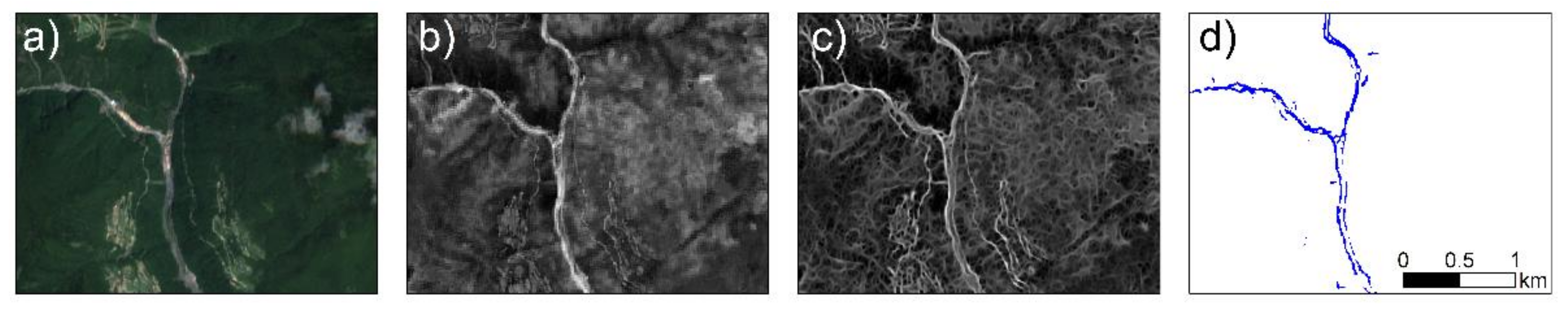
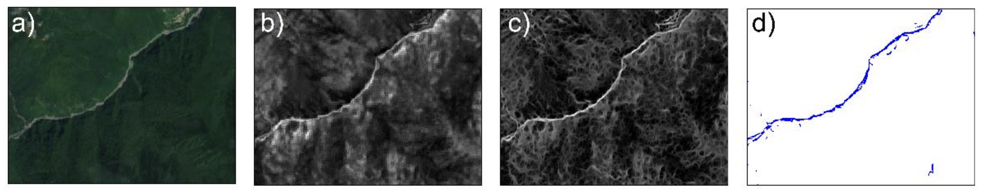
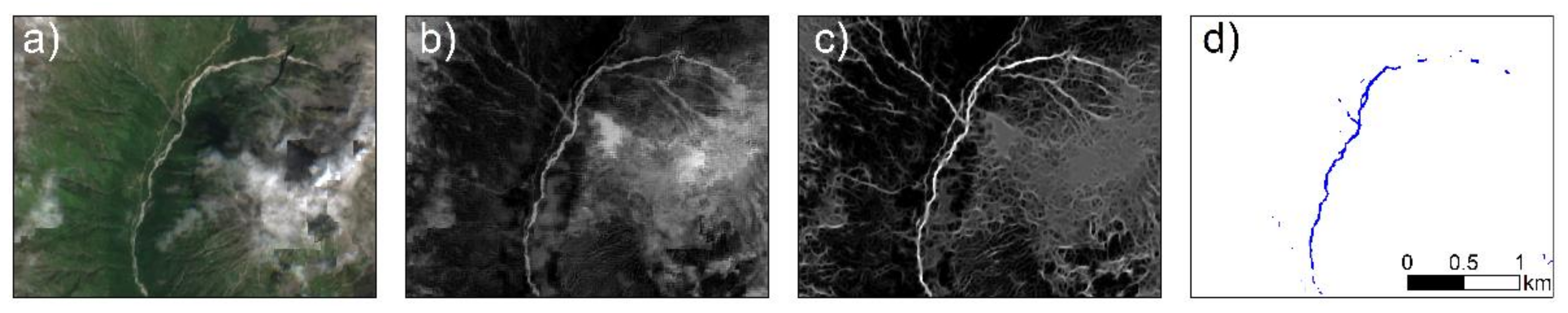
- ASRM achieved an overall accuracy of 87.5%, with more leakage of river pixels than misclassifications. The ASRM performed well in the presence of residential areas, mountain shadows, and cloud cover.
- (2)
- Compared to five existing remote sensing products, ASRM identified more small rivers, providing more detailed and consistent maps. The Drainage density (Dd) of ASRM was more than six times that of other datasets, and the Open Water Fraction (OWF) was more than 1.9 times that of other datasets.
- (3)
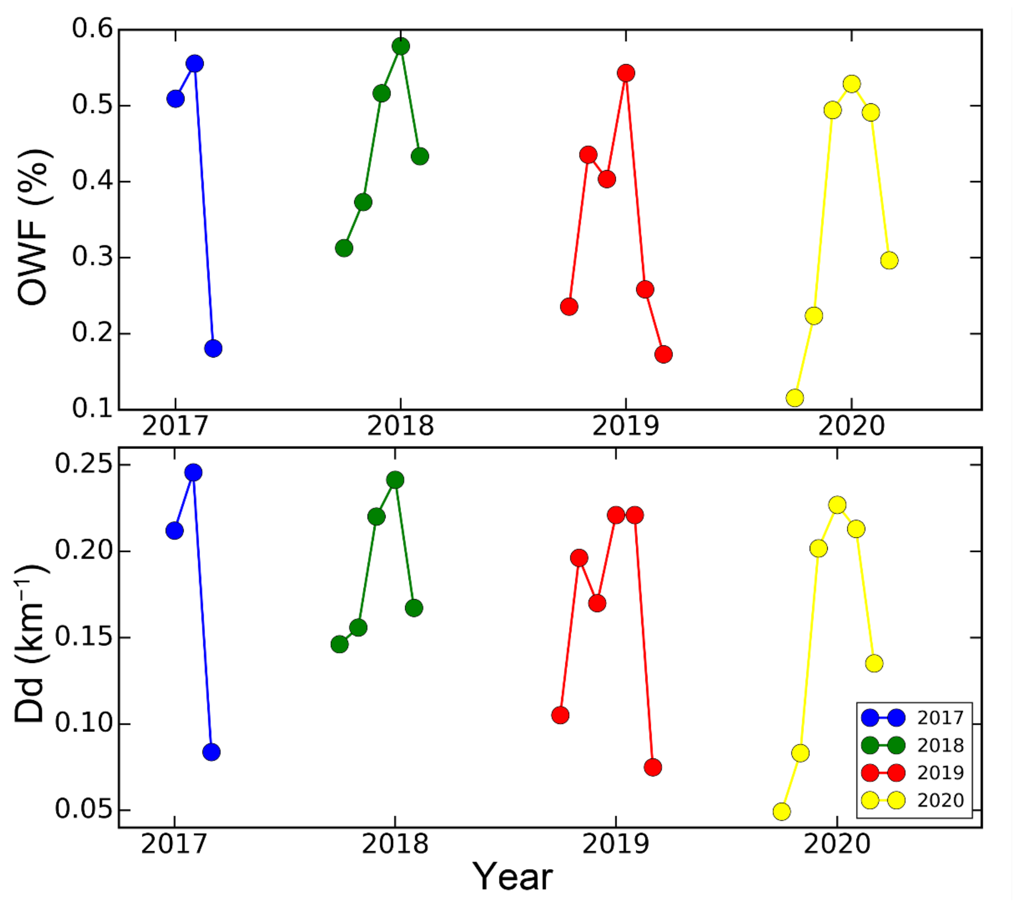
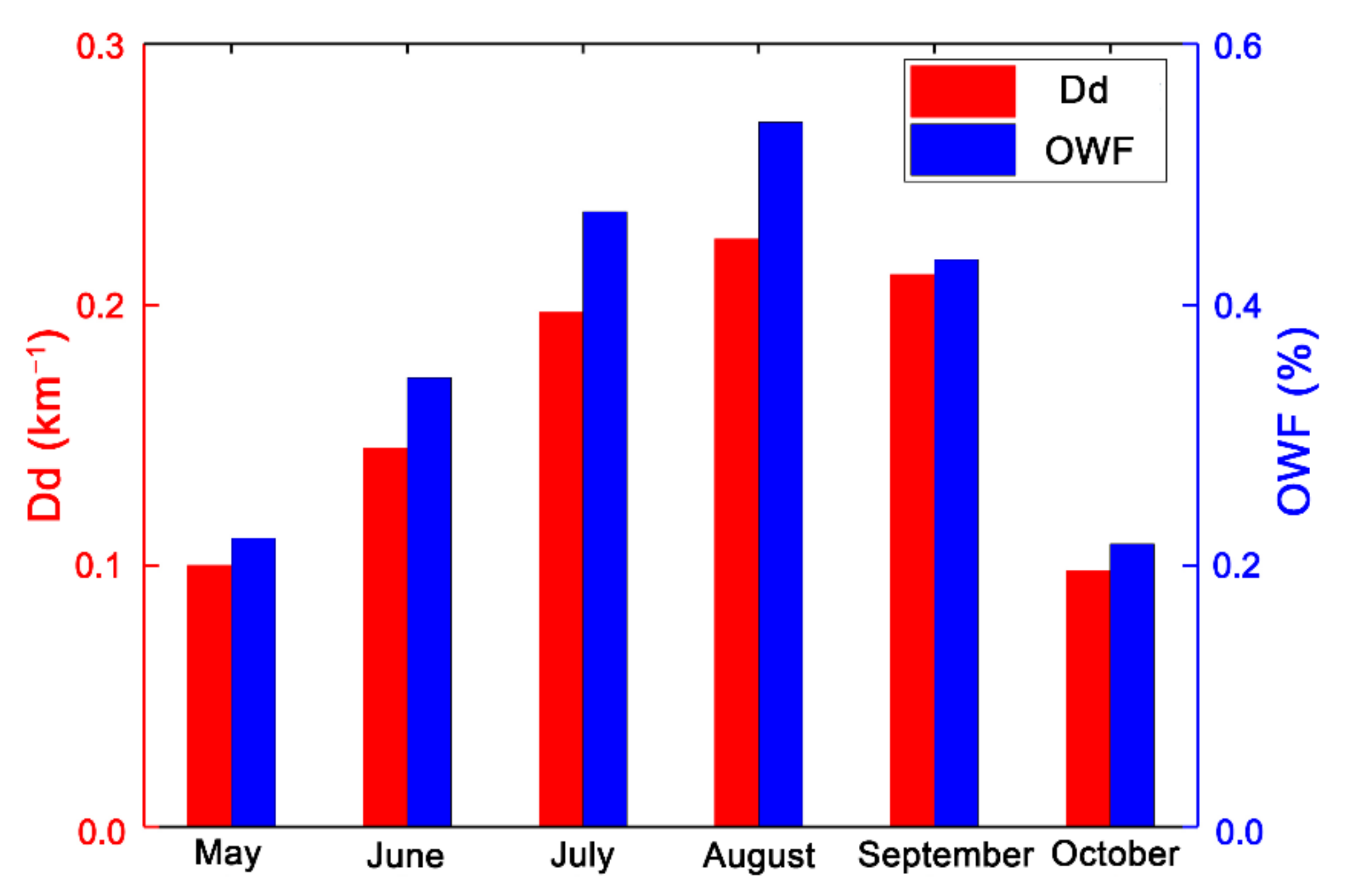
- From the perspective of interannual variations, the annual variations of maximum Dd and OWF of the river networks in the study area were less than 15% from 2017 to 2020. In terms of the seasonal variations, both Dd and OWF increased from May to August, and decreased monthly after August.
Author Contributions
Funding
Data Availability Statement
Conflicts of Interest
References
- Benstead, J.P.; Leigh, D.S. An expanded role for river networks. Nat. Geosci. 2012, 5, 678–679. [Google Scholar] [CrossRef]
- Raymond, P.A.; Hartmann, J.; Lauerwald, R.; Sobek, S.; McDonald, C.; Hoover, M.; Butman, D.; Striegl, R.; Mayorga, E.; Humborg, C.J.N. Global carbon dioxide emissions from inland waters. Nature 2013, 503, 355–359. [Google Scholar] [CrossRef] [PubMed]
- Sjögersten, S.; Black, C.R.; Evers, S.; Hoyos-Santillan, J.; Wright, E.L.; Turner, B.L. Tropical wetlands: A missing link in the global carbon cycle? Glob. Biogeochem. Cycles 2014, 28, 1371–1386. [Google Scholar] [CrossRef] [PubMed]
- Jung, M.; Reichstein, M.; Ciais, P.; Seneviratne, S.I.; Sheffield, J.; Goulden, M.L.; Bonan, G.; Cescatti, A.; Chen, J.; De Jeu, R.J.N. Recent decline in the global land evapotranspiration trend due to limited moisture supply. Nature 2010, 467, 951–954. [Google Scholar] [CrossRef] [PubMed]
- Gudmundsson, L.; Boulange, J.; Do, H.X.; Gosling, S.N.; Grillakis, M.G.; Koutroulis, A.G.; Leonard, M.; Liu, J.; Müller Schmied, H.; Papadimitriou, L.J.S. Globally observed trends in mean and extreme river flow attributed to climate change. Science 2021, 371, 1159–1162. [Google Scholar] [CrossRef]
- Buffington, J.M.; Montgomery, D.R. Geomorphic Classification of Rivers. In Treatise on Geomorphology; Shroder, J.F., Ed.; Academic Press: San Diego, CA, USA, 2013; pp. 730–767. [Google Scholar] [CrossRef]
- Nardini, A.; Brierley, G. Automatic river planform identification by a logical-heuristic algorithm. Geomorphology 2021, 375, 107558. [Google Scholar] [CrossRef]
- Witkowski, K. Reconstruction of Nineteenth-Century Channel Patterns of Polish Carpathians Rivers from the Galicia and Bucovina Map (1861–1864). Remote Sens. 2021, 13, 5147. [Google Scholar] [CrossRef]
- Allen, G.H.; Pavelsky, T.M. Patterns of river width and surface area revealed by the satellite-derived North American River Width data set. Geophys. Res. Lett. 2015, 42, 395–402. [Google Scholar] [CrossRef]
- Alsdorf, D.E.; Rodríguez, E.; Lettenmaier, D.P. Measuring surface water from space. Rev. Geophys. 2007, 45, RG2002. [Google Scholar] [CrossRef]
- Gleason, C.J.; Smith, L.C. Toward global mapping of river discharge using satellite images and at-many-stations hydraulic geometry. Proc. Natl. Acad. Sci. USA 2014, 111, 4788. [Google Scholar] [CrossRef]
- Yamazaki, D.; Trigg, M.A.; Ikeshima, D. Development of a global ~90 m water body map using multi-temporal Landsat images. Remote Sens. Environ. 2015, 171, 337–351. [Google Scholar] [CrossRef]
- Gong, P.; Liu, H.; Zhang, M.; Li, C.; Wang, J.; Huang, H.; Clinton, N.; Ji, L.; Li, W.; Bai, Y.; et al. Stable classification with limited sample: Transferring a 30-m resolution sample set collected in 2015 to mapping 10-m resolution global land cover in 2017. Sci. Bull. 2019, 64, 370–373. [Google Scholar] [CrossRef]
- Pekel, J.-F.; Cottam, A.; Gorelick, N.; Belward, A.S. High-resolution mapping of global surface water and its long-term changes. Nature 2016, 540, 418–422. [Google Scholar] [CrossRef] [PubMed]
- Allen, G.H.; Pavelsky, T.M.J.S. Global extent of rivers and streams. Science 2018, 361, 585–588. [Google Scholar] [CrossRef] [PubMed]
- Hossain, A.A.; Mathias, C.; Blanton, R.J.R.S. Remote sensing of turbidity in the Tennessee River using Landsat 8 satellite. Remote Sens. 2021, 13, 3785. [Google Scholar] [CrossRef]
- Huang, J.; Zhang, Y.; Bing, H.; Peng, J.; Dong, F.; Gao, J.; Arhonditsis, G.B.J.W.R. Characterizing the river water quality in China: Recent progress and on-going challenges. Water Res. 2021, 201, 117309. [Google Scholar] [CrossRef]
- Meyer, J.L.; Strayer, D.L.; Wallace, J.B.; Eggert, S.L.; Helfman, G.S.; Leonard, N.E. The contribution of headwater streams to biodiversity in river networks. Jawra J. Am. Water Resour. Assoc. 2010, 43, 86–103. [Google Scholar] [CrossRef]
- Allen, G.H.; Pavelsky, T.M.; Barefoot, E.A.; Lamb, M.P.; Butman, D.; Tashie, A.; Gleason, C.J. Similarity of stream width distributions across headwater systems. Nat. Commun. 2018, 9, 610. [Google Scholar] [CrossRef]
- Mao, W.; Yang, K.; Zhang, W.; Wang, Y.; Li, M. High-resolution global water body datasets underestimate the extent of small rivers. Int. J. Remote Sens. 2022, 43, 4315–4330. [Google Scholar] [CrossRef]
- Wang, S. Progresses in Variability of Snow Cover over the Qinghai-Tibetan Plateau and Its Impact on Water Resources in China. Plateau Meteorol. 2017, 36, 1153–1164. [Google Scholar]
- Jiang, W.; Niu, Z.; Wang, L.; Yao, R.; Gui, X.; Xiang, F.; Ji, Y.J.R.S. Impacts of Drought and Climatic Factors on Vegetation Dynamics in the Yellow River Basin and Yangtze River Basin, China. Remote Sens. 2022, 14, 930. [Google Scholar] [CrossRef]
- Krause, S.; Abbott, B.W.; Baranov, V.; Bernal, S.; Blaen, P.; Datry, T.; Drummond, J.; Fleckenstein, J.H.; Velez, J.G.; Hannah, D.M.J.W.R.R. Organizational principles of hyporheic exchange flow and biogeochemical cycling in river networks across scales. Water Resour. Res. 2022, 58, e2021WR029771. [Google Scholar] [CrossRef]
- Wei, H.; Xue, D.; Huang, J.; Liu, M.; Li, L.J.R.S. Identification of Coupling Relationship between Ecosystem Services and Urbanization for Supporting Ecological Management: A Case Study on Areas along the Yellow River of Henan Province. Remote Sens. 2022, 14, 2277. [Google Scholar] [CrossRef]
- Luo, J.; Niu, F.; Lin, Z.; Liu, M.; Yin, G. Thermokarst lake changes between 1969 and 2010 in the Beilu River Basin, Qinghai–Tibet Plateau, China. Sci. Bull. 2015, 60, 556–564. [Google Scholar] [CrossRef]
- Li, D.; Wang, G.; Qin, C.; Wu, B.J.R.S. River extraction under bankfull discharge conditions based on sentinel-2 imagery and DEM data. Remote Sens. 2021, 13, 2650. [Google Scholar] [CrossRef]
- Chinese Academy of Sciences. China Natrual Geoscience: Groundwater; Chinese Academy of Sciences: Beijing, China, 1981. [Google Scholar]
- Drusch, M.; Del Bello, U.; Carlier, S.; Colin, O.; Fernandez, V.; Gascon, F.; Hoersch, B.; Isola, C.; Laberinti, P.; Martimort, P.; et al. Sentinel-2: ESA’s Optical High-Resolution Mission for GMES Operational Services. Remote Sens. Environ. 2012, 120, 25–36. [Google Scholar] [CrossRef]
- Bertini, F.; Brand, O.; Carlier, S.; Bello, U.D.; Pieiro, J. Sentinel-2 ESA’s Optical High-Resolution Mission for GMES Operational Services. Remote Sens. Environ. 2012, 120, 25–36. [Google Scholar]
- Meer, F.; Werff, H.; Ruitenbeek, F. Potential of ESA’s Sentinel-2 for geological applications. Remote Sens. Environ. 2014, 148, 124–133. [Google Scholar] [CrossRef]
- Yamazaki, D.; Ikeshima, D.; Sosa, J.; Bates, P.D.; Allen, G.H.; Pavelsky, T.M. MERIT Hydro: A High-Resolution Global Hydrography Map Based on Latest Topography Dataset. Water Resour. Res. 2019, 55, 5053–5073. [Google Scholar] [CrossRef]
- Yamazaki, D.; Ikeshima, D.; Tawatari, R.; Yamaguchi, T.; O’Loughlin, F.; Neal, J.C.; Sampson, C.C.; Kanae, S.; Bates, P.D. A high-accuracy map of global terrain elevations. Geophys. Res. Lett. 2017, 44, 5844–5853. [Google Scholar] [CrossRef]
- Nobre, A.D.; Cuartas, L.A.; Hodnett, M.; Rennó, C.D.; Rodrigues, G.; Silveira, A.; Saleska, S. Height Above the Nearest Drainage–a hydrologically relevant new terrain model. J. Hydrol. 2011, 404, 13–29. [Google Scholar] [CrossRef] [Green Version]
- Lu, X.; Yang, K.; Bennett, M.M.; Liu, C.; Mao, W.; Li, Y.; Zhang, W.; Li, M. High-resolution satellite-derived river network map reveals small Arctic river hydrography. Environ. Res. Lett. 2021, 16, 054015. [Google Scholar] [CrossRef]
- Lehner, B.; Verdin, K.; Jarvis, A. New global hydrography derived from spaceborne elevation data. Eos Trans. Am. Geophys. Union AGU 2008, 89, 93–94. [Google Scholar] [CrossRef]
- McFeeters, S.K. The use of the Normalized Difference Water Index (NDWI) in the delineation of open water features. Int. J. Remote Sens. 1996, 17, 1425–1432. [Google Scholar] [CrossRef]
- Xu, H. Modification of normalised difference water index (NDWI) to enhance open water features in remotely sensed imagery. Int. J. Remote Sens. 2006, 27, 3025–3033. [Google Scholar] [CrossRef]
- Liu, J.-L.; Feng, D.-Z. Two-dimensional multi-pixel anisotropic Gaussian filter for edge-line segment (ELS) detection. Image Vis. Comput. 2014, 32, 37–53. [Google Scholar] [CrossRef]
- Yang, K.; Li, M.; Liu, Y.; Cheng, L.; Huang, Q.; Chen, Y. River detection in remotely sensed imagery using Gabor filtering and path opening. Remote Sens. 2015, 7, 8779–8802. [Google Scholar] [CrossRef]
- Lu, X.; Yang, K.; Lu, Y.; Gleason, C.J.; Li, M. Small Arctic rivers mapped from Sentinel-2 satellite imagery and ArcticDEM. J. Hydrol. 2020, 584, 124689. [Google Scholar] [CrossRef]


| Name | Data Source | Resolution | Introduction | Reference |
|---|---|---|---|---|
| FROM-GLC10 | Sentinel-2 MSI | 10 m | Global land cover data products | Gong et al., 2019 [13] |
| GSW | Landsat MSS/TM/ETM+/OLI | 30 m | Long time series monthly surface water cover | Pekel et al., 2016 [14] |
| GRWL | Landsat MSS/TM/ETM+/OLI | 30m | Vector data product with river width | Allen et al., 2018 [15] |
| OSM | Aerial, satellite imagery, GPS devices and in situ observation data | None | Vector data product based on opensource community contributions | https://www.openstreetmap.org/, accessed on 1 January 2021 |
| HydroSHEDS | SRTM DEM | 450, 900 m | Continuous river networks generated by DEM | Lehner et al., 2008 [35] |
| Background | River | Overall | User Accuracy | |
|---|---|---|---|---|
| Background | 62,194 | 15,197 | 77,391 | 80.36% |
| River | 1909 | 58,057 | 59,966 | 96.82% |
| Overall | 64,103 | 73,254 | 137,357 | |
| Producer Accuracy | 97.02% | 79.25% | ||
| Total accuracy: 87.5% Kappa coefficient: 0.75 | ||||
| Product | Producer Accuracy | User Accuracy | Total Accuracy |
|---|---|---|---|
| ASRM 1 | 79.25% | 96.82% | 87.5% |
| FROM-GLC10 | 4.8% | 92.9% | 59.0% |
| GSW | 37.1% | 93.2% | 69.6% |
| GRWL | 11.6% | 100.0% | 57.0% |
| Date | OWF (%) | Dd (km−1) |
|---|---|---|
| 2017/08 | 0.51 | 0.21 |
| 2017/09 | 0.56 | 0.25 |
| 2017/10 | 0.18 | 0.08 |
| 2018/06 | 0.37 | 0.16 |
| 2018/07 | 0.52 | 0.22 |
| 2018/08 | 0.58 | 0.24 |
| 2018/09 | 0.43 | 0.17 |
| 2019/05 | 0.24 | 0.11 |
| 2019/06 | 0.44 | 0.20 |
| 2019/07 | 0.40 | 0.17 |
| 2019/08 | 0.54 | 0.22 |
| 2019/09 | 0.26 | 0.22 |
| 2019/10 | 0.17 | 0.07 |
| 2020/05 | 0.12 | 0.05 |
| 2020/06 | 0.22 | 0.08 |
| 2020/07 | 0.49 | 0.20 |
| 2020/08 | 0.53 | 0.23 |
| 2020/09 | 0.49 | 0.21 |
| 2020/10 | 0.30 | 0.13 |
| Month | OWF (%) | Dd (km−1) |
|---|---|---|
| May | 0.22 | 0.10 |
| June | 0.34 | 0.15 |
| July | 0.47 | 0.20 |
| August | 0.54 | 0.23 |
| September | 0.43 | 0.21 |
| October | 0.22 | 0.10 |
Publisher’s Note: MDPI stays neutral with regard to jurisdictional claims in published maps and institutional affiliations. |
© 2022 by the authors. Licensee MDPI, Basel, Switzerland. This article is an open access article distributed under the terms and conditions of the Creative Commons Attribution (CC BY) license (https://creativecommons.org/licenses/by/4.0/).
Share and Cite
Liang, X.; Mao, W.; Yang, K.; Ji, L. Automated Small River Mapping (ASRM) for the Qinghai-Tibet Plateau Based on Sentinel-2 Satellite Imagery and MERIT DEM. Remote Sens. 2022, 14, 4693. https://doi.org/10.3390/rs14194693
Liang X, Mao W, Yang K, Ji L. Automated Small River Mapping (ASRM) for the Qinghai-Tibet Plateau Based on Sentinel-2 Satellite Imagery and MERIT DEM. Remote Sensing. 2022; 14(19):4693. https://doi.org/10.3390/rs14194693
Chicago/Turabian StyleLiang, Xiangan, Wei Mao, Kang Yang, and Luyan Ji. 2022. "Automated Small River Mapping (ASRM) for the Qinghai-Tibet Plateau Based on Sentinel-2 Satellite Imagery and MERIT DEM" Remote Sensing 14, no. 19: 4693. https://doi.org/10.3390/rs14194693