Assessment of Galileo FOC + IOV Signals and Geometry-Based Single-Epoch Resolution of Quad-Frequency Carrier Ambiguities

Abstract

Galileo can independently provide navigation and positioning services globally. Galileo satellites transmit quad-frequency E1, E5a, E5b, and E5 signals, which can benefit the integer ambiguity rapid resolution. Firstly, the qualities of Galileo signals from Carrier-to-Noise (C/N0), Multipath Combination (MPC), and pseudo-range and phase noise using the ultra-short baseline were evaluated. The experimental results indicated that the Galileo E5 signal has the highest C/N0, while the C/N0 of other signals is lower and almost equal. In terms of MPC, the Galileo E1 was the most severe followed by E5a and E5b, and the MPC of E5 is less severe. As for the precision of un-differenced observations, the carrier phase and pseudo-range observations of Galileo E5 had higher accuracy than those of Galileo E5a, E5b, and E1. Secondly, the quad-frequency observations allowed for various linear combinations of different frequencies, which provides some feasibility for improving the performance of ambiguity resolution. Assuming that the phase noise ${\sigma }_{\nabla \Delta \mathsf{\Phi }} = 0.01 \mathrm{m}$ and the first-order ionosphere ${\sigma }_{\nabla \Delta I_1} = 1 \mathrm{m}$, the total noise of the Extra-Wide-Lane (EWL) combination observation ((0, 0, 1, −1) and (0, −1, 1, 0)) and Very-Wide-Lane (VWL) combination observation ((0, −2, 1, 1), (0, −3, 2, 1)) are still less than 0.5 cycles. Finally, a geometry-based quad-frequency carrier ambiguities (GB-QCAR) method was developed, and all different options of linear combinations were investigated systematically from the ambiguity-fixed rate with two baselines. Experimental results demonstrated that, the ambiguity fixed rate of combination observation (0, −1, 1, 0), (0, −3, 5, −2), (1, −1, 0, 0) and (0, 0, 0, 1) is the highest and the positioning accuracy of VWL combination observation (0, −3, 5, −2) is equivalent to that of the EWL combination observation (0, −1, 1, 0). The positioning accuracies of WL combination observation (1, −1, 0, 0) are preferable to 3 cm and 10 cm in the horizontal and vertical, respectively. The positioning accuracy of NL combination observation E5 in the horizontal direction is about 1 cm, and is better than 4 cm in the vertical direction. Therefore, we can use Galileo observations to realize high-precise navigation services utilizing the proposed GB-QCAR method.

1. Introduction

The European Galileo is being managed in cooperation between the European Union (EU) and the European Space Agency (ESA), which offers precise positioning services [1,2]. From 2005 to 2008, two test Galileo in-orbit validation element (GIOVE) satellites (GIOVE-A and -B) were launched, respectively. The In-Orbit Validation (IOV) satellites were launched in 2011 and 2012, and the first two Full Operational Capability (FOC) satellites were launched in August 2014. Twenty-four Galileo satellites were available to users up to the time of writing, which include 3 IOV and 21 FOC satellites. The full Galileo will consist of 30 satellites in an in-orbit constellation [3,4]. 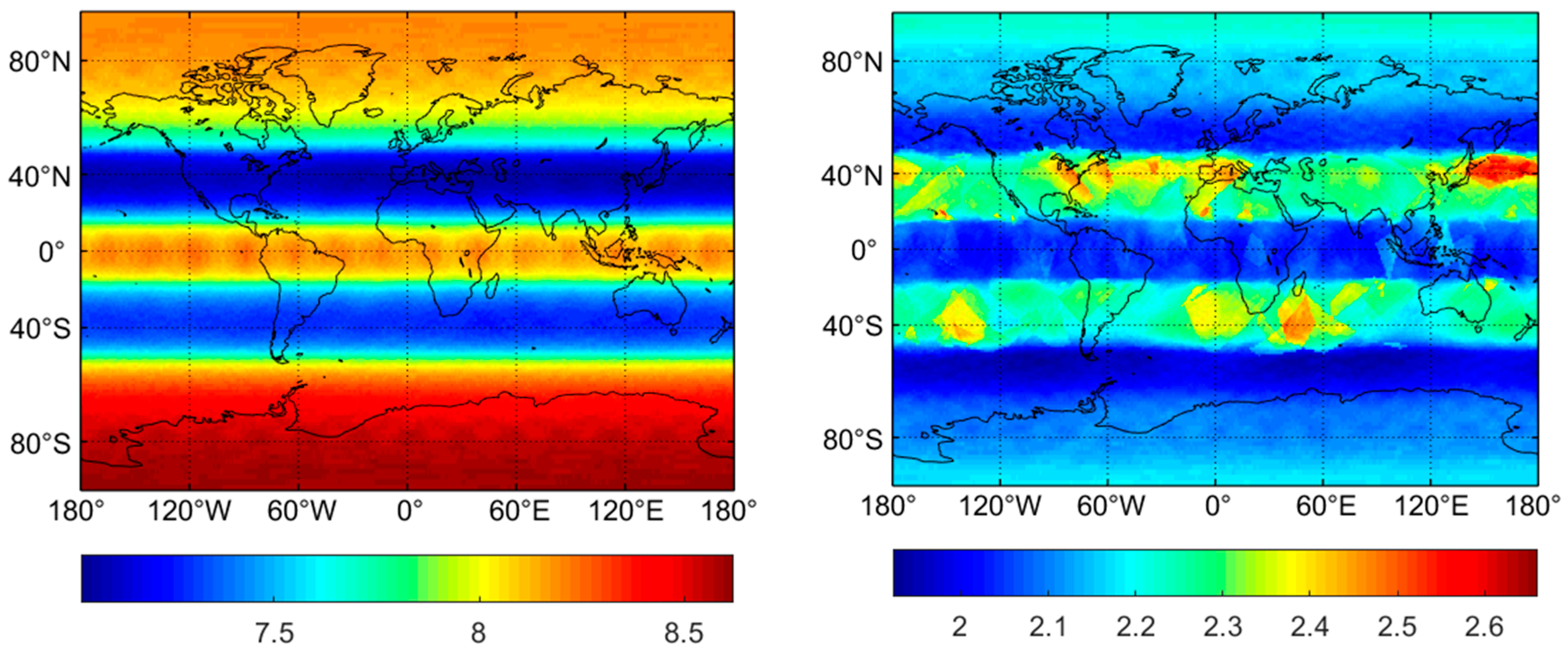Figure 1 shows the number of visible satellites and Position Dilution of Precision (PDOP) values for Galileo. The data span is days of year (DOY) 140–146 of 2019, and the cut-off elevation angle is 10°. From Figure 1, at least six satellites can be observed at a 10° cut-off elevation angle almost everywhere and anytime. Within the scope of the equator and the poles, at least eight satellites were permanently in view. The variety of average PDOP is from 2.0 to 2.6. The Galileo is designed to transmit penta-frequency signals E1, E5a, E5b, E5, and E6, whose frequencies are 1575.420 MHz, 1176.450 MHz, 1207.140 MHz, 1191.795 MHz, and 1278.750 MHz, respectively. In terms of signal quality, Simsky et al. [5,6] used GIOVE-A and -B data to evaluate the multipath combination performance of the Galileo signal.

According to Cai et al.’s [7] study, they showed that the multipath and noise effects of four IOVs have less than GPS satellites. Odijk et al. [8,9] analyzed the performances of ambiguity resolution and positioning under short baselines based on the observations of four IOV satellites combined with GPS. With the development of FOC satellites, Gaglione et al. [10] studied the potential improvements in constellation geometry when adding FOC satellites. To grasp the signal quality of Galileo satellites, Zaminpardaz and Teunissen [11] systematically evaluated the multipath and noise characteristics of four IOV satellites and nine FOC satellites. Their results showed that the E5 signal showed a significantly higher signal power and lower level of multipath and noise among the five Galileo signals. Besides, using the modified multipath data, Galileo E5 can make instantaneous ambiguity resolution feasible. Liu et al. [12] studied the benefit of Galileo E6 signals and their application in precise point positioning (PPP) with ambiguity resolution (AR); the results indicated that the Galileo E6 signal can bring a significant improvement in real-time instantaneous decimeter-level PPP AR. With the continuous development of Galileo, its data has been studied for various Global Navigation Satellite System (GNSS) applications with a single Galileo mode or Galileo fusion with other GNSS modes [13,14]. Diessongo et al. [15] proved that the addition of the Galileo E5 signal further improves the accuracy of pseudo-range measurement and hence enables accurate single-frequency positioning. A comprehensive analysis of position velocity and time (PVT) performance was also performed using a broadcast ephemeris [16]. Odolinski et al. [17] combined the single-frequency signal of GPS, BDS, Galileo, and QZSS to explore whether the performance of real-time kinematic positioning (RTK) is further improved. The results showed that the addition of the Galileo satellite is of great significance to GNSS positioning service. Stochastic properties of GNSS (GPS L1 C/A, L5Q, GIOVE E1B, and E5aQ signals) range measurements can accurately be estimated using a geometry-free short and zero baseline analysis method [18]; the results showed that GPS and Galileo mixed double differenced ambiguities could be resolved with a success rate comparable to single system ambiguities. The Indian Regional Navigation Satellite System (IRNSS) L5-signal in combination with GPS, Galileo, and the Japanese Quasi-Zenith Satellite System (QZSS) L5/E5a-signals for positioning and navigation was assessed by Nadarajah et al. [19]; the results show better ambiguity resolution performance of L5/E5a only processing than that of L1/E1-only processing. Bastos et al. [20] gave a systematic analysis of kinematic Galileo and GPS Performances in Aerial, Terrestrial, and Maritime Environments. Zhao et al. [21] assessed the positioning performance of GPS/BDS-3/GLONASS/Galileo in polar regions; the results indicate the multi-constellation combination slightly improves positioning accuracy, compared to single-constellation. The current performance of open position service with almost fully deployed multi-GNSS constellations: GPS, GLONASS, Galileo, BDS-2, and BDS-3 were evaluated by Zhang et al. [22]; the positioning accuracy of four-system integrated single point positioning (SPP) is 0.484/0.987/2.084, 0.525/0.897/2.340, and 1.932/2.671/8.502 m in the east/north/up directions at a global service rate of 100.0%, 99.8%, and 69.4% under a cut-off elevation angle of 10°, 30°, and 50°, respectively. Chen et al. [23] comprehensively studied the tight integration of BDS-3, GPS, GALILEO, and QZSS overlapping frequencies signals to show its superiority for integer ambiguity resolution and precise positioning, compared to loose integration; the experiments showed that the tight integration can significantly improve ambiguity resolution and positioning accuracy.

In terms of multi-frequency linear combination, the three-frequency carrier ambiguity resolution (TCAR) approach was first proposed by Forssell and Volath [24,25], and its basic principle is to fix extra-wide-lane (EWL) ambiguity, wide-lane (WL) ambiguity, and narrow-lane (NL) ambiguity in turn. Jung et al. [26] presented a method similar to the TCAR method, which is called cascading integer resolution (CIR). Teunissen et al. [27] comprehensively compared the performance of the three methods TCAR, CIR, and least-squares ambiguity decorrelation adjustment (Lambda) method from the perspective of fixed triple-frequency ambiguity, and pointed out that the Lambda method is better than TCAR and CIR model. Feng and Hatch et al. [28,29] extended the TCAR method to the Geometry-based mode (GB), which effectively improved the fixed rate of triple-frequency ambiguity. The performance of BDS-3/GPS/Galileo TCAR based on the geometry-free (GF) model was evaluated by Chen et al. [30]. To summarize, the current multiple carrier ambiguity resolution methods referred to above are characterized to use only triple-frequency to form various EWL observables. To further study the characteristics of the multi-frequency (especially for quad-frequency and penta-frequency) combination observations, evaluations and research have been conducted by many scholars. Zhang et al. [31,32] studied the basic theory and method of the BDS-3 multi-frequency carrier ambiguities resolution (MCAR), including three-frequency, quad-frequency, and penta-frequency carrier ambiguity resolution. The medium-long-baseline RTK single-epoch positioning method based on BDS-3 penta-frequency EWL/WL combinations is proposed by Gao et al. [33]; the experimental results show that the EWL/WL ambiguities of BDS-3 can be fixed reliably in a single epoch. Jin et al. [34] presented multi-GNSS PPP models from single- to penta-frequency observations; the results show that the multi-frequency multi-GNSS has greatly improved the accuracy and reliability of PPP in parameters estimation. Li et al. [35] discussed the benefits of quad-frequency observations; the results indicated that the horizontal positioning errors of EWL real-time kinematic (ERTK) positioning using ionosphere-free (IF) EWL observations are approximately 0.5 m for the baseline of 27 km. Zhang et al. [36] used the quad-frequency ionosphere weighted model for Long Baseline. The results showed that: compared with the double-frequency ionosphere-free model and the triple-frequency geometry-based model, the success rate of the basic ambiguity was increased by the proposed method. The BDS dual- and penta-frequency Precise Point Positioning (PPP) models were comprehensively evaluated by Wu et al. [37] in terms of the static and simulated kinematic positioning performances. The results of the experiment showed that the penta-frequency IF combination model has the best positioning consequent in the static, especially in the up direction. The stepwise ionosphere-free single epoch algorithm based on BDS-3 quad-frequency signals was proposed by Zhang et al. [38]. Li et al. [39] adopted fuzzy clustering analysis to realize the selection of the optimal combination of triple-frequency, quad-frequency, and penta-frequency observations under different baseline lengths. The unified model of GNSS phase/code bias calibration for PPP ambiguity resolution with GPS, BDS, Galileo, and GLONASS multi-frequency observations was developed by Li et al. [40]. Wang and Liu [41] proposed some new combination strategies to fully exploit the quad-frequency of Galileo to form linear combination observables, which have better properties of long-wavelength, weak ionospheric delay, and low measurement noise. Ji et al. [42] investigated the single-epoch ambiguity resolution performance with the Cascade Ambiguity Resolution (CAR) and Lambda methods using Galileo Quad-frequency simulated data. The results proved that the Lambda method is better than the CAR method based on the simulation data. However, the above results are mainly aimed at BDS-3 multi-frequency observations and theoretical analysis of Galileo simulation data. Therefore, it is of great significance to further study the linear combination characteristics of the Galileo quad-frequency observations and select the optimal linear combination observations. Finally, the characteristics of the ambiguity of the different linear combinations through measured data were evaluated.

In this contribution, the quality analysis of signals is expounded first in Section 2. In Section 3, the optimal linear combinations are selected for Galileo quad-frequency observation. A Geometry-based quad-frequency carrier ambiguities (GB-QCAR) method is proposed in detail, and all different options of linear combinations are analyzed systematically with respect to the ambiguity-fixed rate in Section 4. Finally, the conclusions and experimental results are summarized in Section 5.

2. Methods

2.1. Basic Models of Galileo Quad-Frequency Linear Combinations

Assuming that g, h, k, and l are the combination integer coefficients, the combined observation in cycle units is expressed as

$${\phi }_{g,h,k,l}=g\cdot {\phi }_1+h\cdot {\phi }_2+k\cdot {\phi }_3+l\cdot {\phi }_4$$

(1)

where ${\phi }_{g,h,k,l}$ denotes carrier phase combination observation; ${\phi }_1,{\phi }_2,{\phi }_3,{\phi }_4$ denote the first, second, third, and quad frequency of corresponding E1, E5a, E5b, and E5, respectively. The frequency $f_{g,h,k,l}$, wavelength ${\mathit{\lambda }}_{g,h,k,l}$ and ambiguity $N_{g,h,k,l}$ of the combination observation can be written as follows:

$$\left\{\begin{array}{l}{f}_{g,h,k,l}=g\cdot f_1+h\cdot f_2+k\cdot f_3+l\cdot f_4\\ {\mathit{\lambda }}_{g,h,k,l}=\mathrm{C}/f_{g,h,k,l}\\ N_{g,h,k,l}=g\cdot N_1+h\cdot N_2+k\cdot N_3+l\cdot N_4\end{array}\right.$$

(2)

where $f_1,f_2,f_3,f_4$ denote the frequency of corresponding carrier phase observation, respectively; $N_1,N_2,N_3,N_4$ denote the ambiguity of corresponding carrier phase observation, respectively; C stands for the speed of light.

The first-order ionospheric delay scale factor of the combination observations can be expressed as:

$${\eta }_{g,h,k,l}=\frac{g+h\frac{f_1}{f_2}+k\frac{f_1}{f_3}+l\frac{f_1}{f_4}}{g+h\frac{f_2}{f_1}+k\frac{f_3}{f_1}+l\frac{f_4}{f_1}}$$

(3)

Assuming that ${\epsilon }_{{\phi }_1}^2={\epsilon }_{{\phi }_2}^2={\epsilon }_{{\phi }_3}^2={\epsilon }_{{\phi }_4}^2={\epsilon }_0^2$, the noise of the carrier phase combination observations is:

$${\epsilon }_{{\phi }_{g,h,k,l}}=\sqrt{g^2+h^2+k^2+l^2}{\epsilon }_0$$

(4)

2.2. Optimal Linear Combination

The combined observation wavelength is crucial to determine the ambiguity. The longer the combined observation wavelength, the easier it is to fix the ambiguity. In this section, Galileo quad-frequency combined observations were selected with the criteria of longer wavelength and less noise. Long-wavelength combined observations should satisfy:

$${\lambda }_{g,h,k,l}=\frac{{\lambda }_1{\lambda }_2{\lambda }_3{\lambda }_4}{g{\lambda }_2{\lambda }_3{\lambda }_4+h{\lambda }_1{\lambda }_3{\lambda }_4+k{\lambda }_1{\lambda }_2{\lambda }_4+l{\lambda }_1{\lambda }_2{\lambda }_3}>{\lambda }_4$$

(5)

According to Equation (9), we can obtain the inequality:

$$1-(ug+yh+zk)>l>-(ug+yh+zk)$$

(6)

where the values of u, y, and z are: $u={\lambda }_4/{\lambda }_1=154/115,y={\lambda }_4/{\lambda }_2=118/115,$$z={\lambda }_4/{\lambda }_3=233/230$.

To ensure that d is an integer, then

$$l=[-(ug+yh+zk\left)\right]$$

(7)

where $\left[(\cdot )\right]$ denote round function for $+\infty$ direction.

The wavelength of the combined observation is:

$${\lambda }_{g,h,h,l}=\frac{{\lambda }_4}{(ug+yh+zk)+[-(ug+yh+zk\left)\right]}$$

(8)

Since Equation (8) is a periodic function:

$$\begin{array}{l}(ug+yh+zk)+[-(ug+yh+zk\left)\right]=\\ \left(u\right(g+P_1)+y(h+P_2)+z(k+P_3\left)\right)+[-u(g+P_1)+y(h+P_2)+z(k+P_3\left)\right)]\end{array}$$

(9)

Since u, y, z are specific values, the periods of g, h, k are $P_1=115,P_2=115,P_3=230$, respectively; according to Equation (4), the absolute values of g, h, k, and l should be made as small as possible to make the noise of the combined observations smaller. Therefore, the range of the combined coefficients is obtained as $g\in \left[-57,58\right],h\in \left[-57,58\right],$$k\in \left[-114,116\right]$.

Considering the effects of phase noises ${\sigma }_{\nabla \Delta \mathsf{\Phi }}$ and first-order ionosphere errors ${\eta }_{\nabla \Delta I_1}$, the total noise level ${\sigma }_{com}$ can be expressed as:

$${\sigma }_{com}=\frac{1}{{\lambda }_{g,h,k,l}}\sqrt{{\eta }_{g,h,k,l}^2{\eta }_{\nabla \Delta I_1}^2+{\epsilon }_{g,h,k,l}^2{\epsilon }_{\nabla \Delta \mathsf{\Phi }}^2}$$

(10)

The quad-frequency phase combination can be divided into four categories: Extra-Wide-Lane ($\lambda \ge 9.768 \mathrm{m}$, EWL), Very-Wide-Lane ($2.442 \mathrm{m}\le \lambda <9.768 \mathrm{m}$, VWL), Wide-Lane ($0.751 \mathrm{m}\le \lambda <2.442 \mathrm{m}$, WL), Narrow-Lane ($\lambda <0.19 \mathrm{m}$, NL). Assuming that ${\sigma }_{\nabla \Delta \mathsf{\Phi }}=0.01 \mathrm{m}$, the Galileo quad-frequency combination observation characteristics are shown in

Table 1. Characteristics of typical Galileo quad-frequency combined observations.

g	h	k	l	${\mathit{\lambda }}_{\mathit{k},\mathit{l},\mathit{m},\mathit{n}}/\mathbf{m}$	${\mathit{\eta }}_{\mathit{k},\mathit{l},\mathit{m},\mathit{n}}$	${\mathit{u}}_{\mathit{k},\mathit{l},\mathit{m},\mathit{n}}$	${\mathit{\sigma }}_{\mathit{c}\mathit{o}\mathit{m}}/\mathbf{Cycle}$
							$\nabla \Delta {\mathit{I}}_1=0.02 \mathbf{m}$	$\nabla \Delta {\mathit{I}}_1=1 \mathbf{m}$
0	0	1	−1	19.537	−1.726	110.547	0.057	0.105
0	−1	1	0	9.768	−1.748	54.923	0.056	0.188
0	−2	1	1	6.512	−1.755	63.009	0.097	0.286
0	−3	2	1	3.907	−1.752	57.857	0.148	0.472
0	−4	3	1	2.791	−1.751	56.383	0.202	0.659
0	−3	5	−2	2.442	−1.742	60.174	0.285	0.755
1	2	−4	1	1.028	−1.190	19.629	0.192	1.173
1	0	−1	0	0.814	−1.305	5.389	0.074	1.605
1	0	0	−1	0.781	−1.321	5.149	0.074	1.693
1	−1	0	0	0.751	−1.339	4.923	0.075	1.783

. Table 1 shows that the total noise from combined observations is less than 1 cycle when the first-order ionospheric error is 0.02 m. When the first-order ionospheric error is 1 m, the total noise of the EWL combination ((0, 0, 1, −1) and (0, −1, 1, 0)) and the VWL combination ((0, −2, 1, 1), (0, −3, 2, 1), (0, −4, 3, 1) and (0, −3, 5, −2)) are still less than 1 cycle. The advantage of long-wavelength combined observation is that the ambiguity is easy to fix. The wavelengths of EWL combination (0, 0, 1, −1) and (0, −1, 1, 0) are 19.537 m and 9.768 m, respectively, and the total noise is less than 0.2 cycles. In the combination of VWL, the combination (0, −2, 1, 1) has the longest wavelength and the noise is less than 0.3 cycles.

3. Results

3.1. Carrier-to-Noise Density Ratio and Multipath Combination of Galileo Signals

To study the performance of different signals, the quality in terms of carrier-to-noise density ratio (C/N0) and multipath combination (MPC) were performed in this section. The observation data collection time was 7 days, which were days of the year (DOY 350–356, 2018) in the case of CUT0 and UWA0 stations. The receiver types of the two stations are TRIMBLE NETR9 (Trimble Inc., Sunnyvale, CA, USA) and SEPT POLARX5 (Septentrio, Leuven, Belgium), and are located at Curtin University, Perth, Australia. The sampling interval of observation data was 30 s.

The quality of the satellite signal has a certain relationship with the C/N0 value.

Table 2. Galileo frequencies and wavelengths.

Signal	Frequency (MHz)	Wavelength (m)	Bandwidth (MHz)	Modulation Scheme
E1	1575.420	0.1903	24.552	CBOC
E5a	1176.450	0.2548	20.460	BPSK
E5b	1207.140	0.2483	20.460	BPSK
E5	1191.795	0.2515	51.150	AltBoc

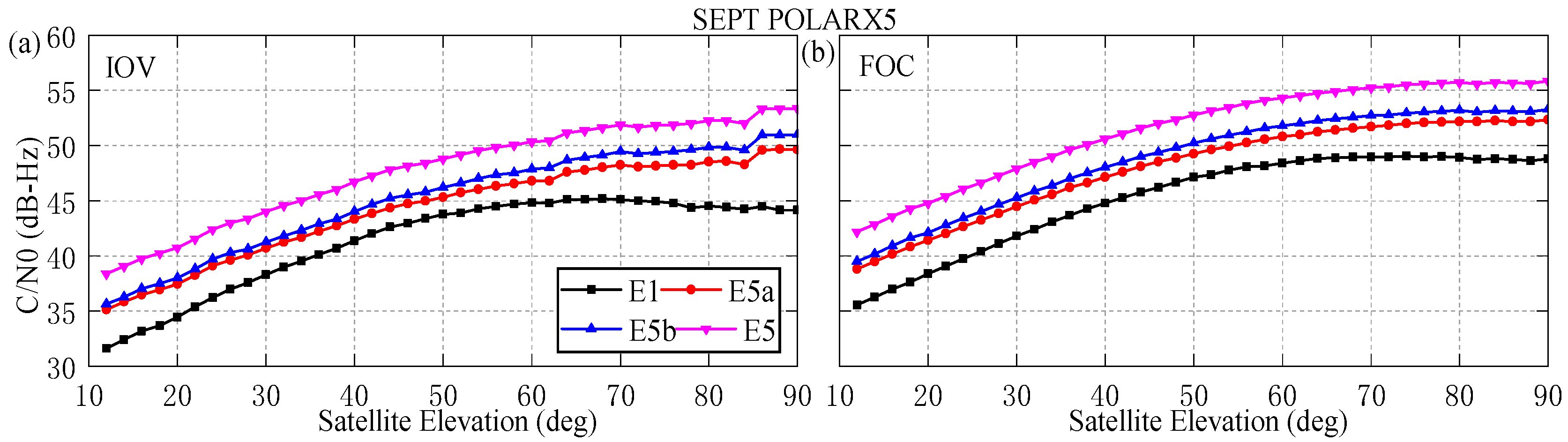
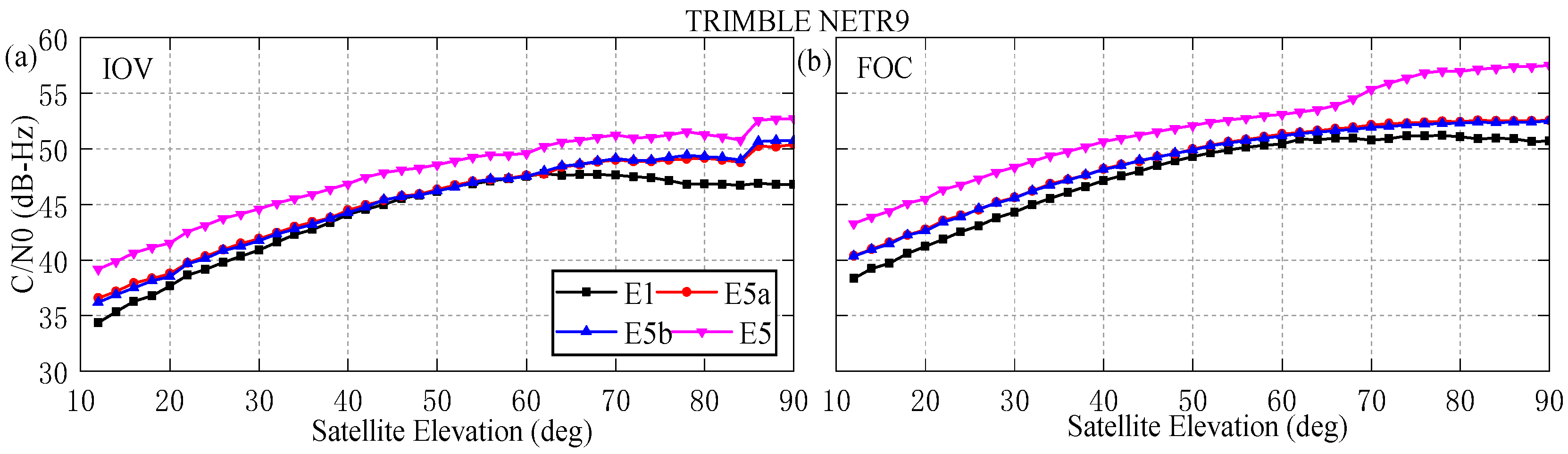
gives the Galileo signals tracked by CUT0 and UWA0 stations. From Table 1, the E1 signal adopts the Composite Binary Offset Carrier (CBOC) modulation scheme. The E5 signal with the widest bandwidth applies Alternate Binary Offset Carrier (AltBOC) modulation and is composed of two subcarriers, E5a and E5b, tracked as two independent Binary Phase Shift Keying (BPSK) modulations. In this study, the C/N0 values of each satellite signal are segmented to take the averaging value according to the elevation interval of 2°. To compare the C/N0 of different signals for the same type of satellite, Figure 2 and Figure 3 show the C/N0 of the Galileo signals relative to elevation for the different receiver types. Figure 2 and Figure 3 show that the higher cut-off elevation angle corresponds to the higher C/N0 values, and vice versa. For the same type of satellite, the C/N0 values of the E5 signal are the best at all frequencies, while the E1 signal is the worst. The C/N0 values of all frequencies are above 30. When the cut-off elevation angle is greater than 70°, the change in the C/N0 value is not obvious. For the receiver type TRIMBLE NETR9, the C/N0 values of the E5a and E5b signals are basically equivalent.

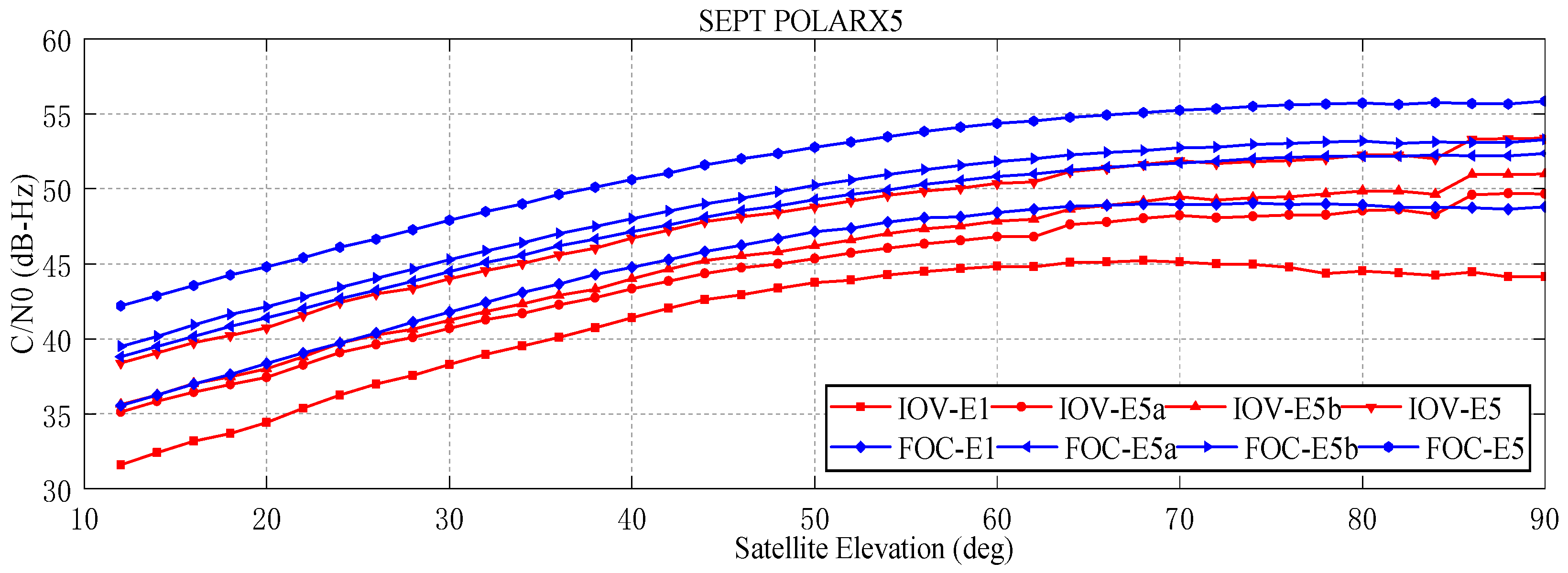
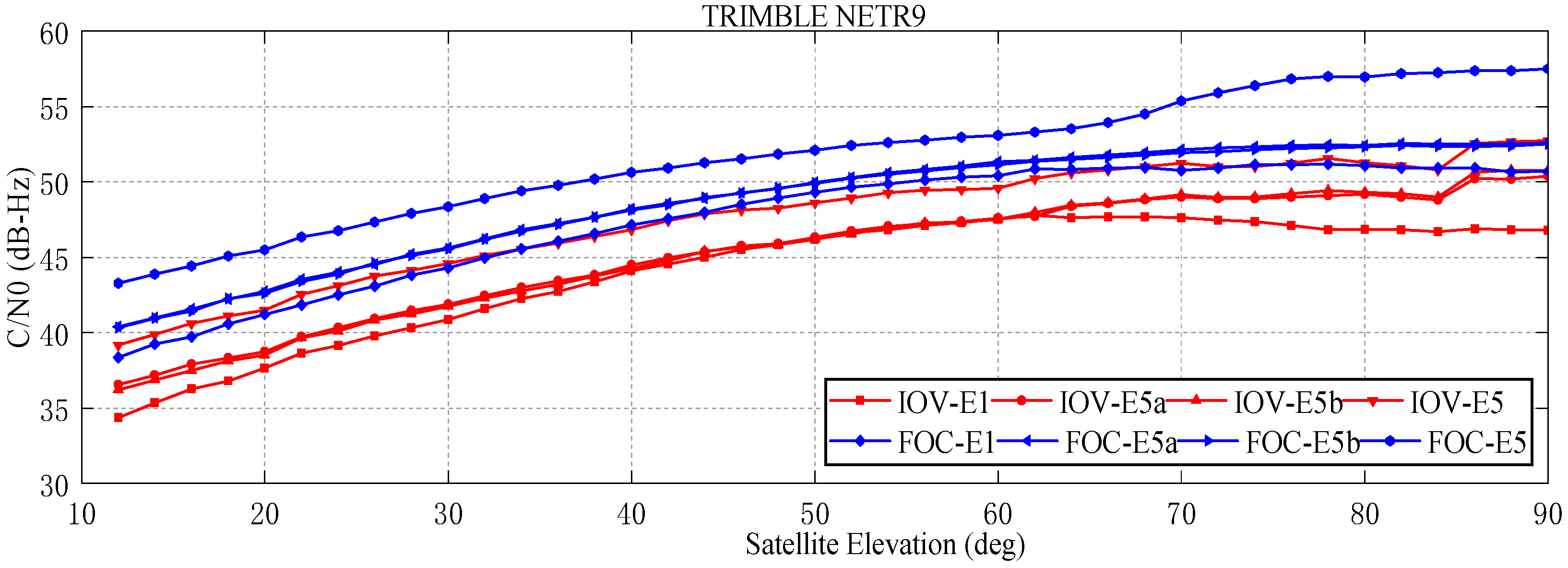
To further evaluate the C/N0 of the same signal with different satellite types, the C/N0 values of the two receiver types SEPT POLARX5 and TRIMBLE NETR9 are described in Figure 4 and Figure 5, respectively. For the two receiver types, the C/N0 values of the FOC E5 signal perform the best in all frequencies, while the IOV E1 signal is the worst. At the same cut-off elevation angle, the C/N0 value from the FOC satellites is 3~4 dB-Hz higher than that of the IOV satellites at all four signals. This difference may be due to the differences in transmit antenna mode and transmit power level between FOC and IOV satellites.

MPC is usually used to evaluate pseudo-range multipath. MPC is expressed as follows

$${\mathrm{MPC}}_i^s=P_{r,i}^s-\frac{f_i^2+f_j^2}{f_i^2-f_j^2}{\mathsf{\Phi }}_{r,i}^s+\frac{2f_j^2}{f_i^2-f_j^2}{\mathsf{\Phi }}_{r,j}^s=M_{r,i}^s-\frac{f_i^2+f_j^2}{f_i^2-f_j^2}{m}_{r,i}^s+\frac{2f_j^2}{f_i^2-f_j^2}{m}_{r,j}^s+B_{r,i}^s+{\epsilon }_{r,i}^s$$

(11)

where $P_{r,i}^s$ and ${\mathsf{\Phi }}_{r,i}^s$ denote the pseudo-range and carrier phase observations from receiver r to satellite s, respectively. f is the carrier phase frequency, and i, j are the subscripts of carrier phase frequency. $M_{r,i}^s$ and $m_{r,i}^s$ denote the pseudo-range multipath and carrier phase multipath, respectively. ${\mathit{\epsilon }}_{r,i}^s$ is noise of combined observation. $B_{i,j}$ contains phase ambiguity and hardware bias.

All geometric contributions (clocks, orbits and antenna movements, etc.), tropospheric delay, and first-order ionosphere delay are all eliminated in the MPC. Then the remaining terms in MPC include phase ambiguity, hardware bias, multipath, and observation noise. In general, the hardware delay remains stable for a certain period of time, and the phase ambiguity maintains a constant in a continuous arc period without cycle slips. Therefore, the constant term B can be derived by averaging the MPC values in a continuous arc. After subtracting term B from MPC, the MPC only contains the observation noise and multipath. Since the phase multipath is far less than the pseudo-range multipath, the pseudo-range multipath characteristics can be analyzed by MPC. For the MPCs of E5a, E5b, and E5, the E1 is selected as the input of carrier phase observation, and the MPC for E1 adopts the E5 as the additional carrier phase observation. 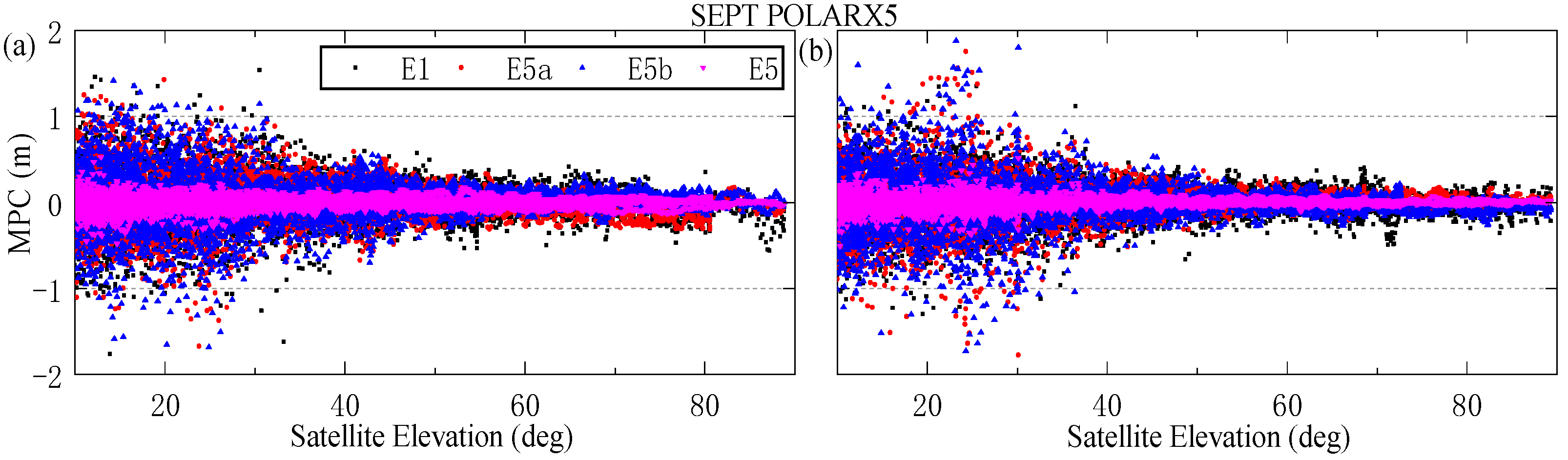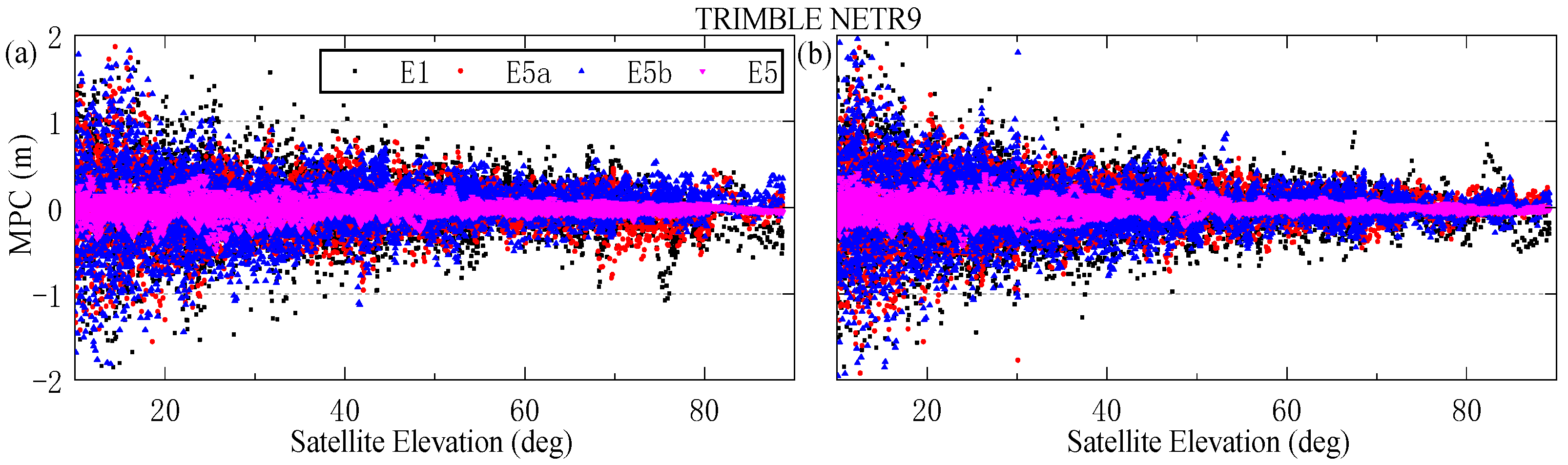Figure 6 and Figure 7 depict the MPC values against satellite elevation of different Galileo satellites (IOV-E12, FOC-E04) for different receiver types. It can be seen from the figure that the fluctuation range of MPC is within $\pm$2 m for different types of satellites. E5 frequency is significantly smaller than other signals in terms of MPC value. The MPC value is large at low cut-off elevation angles, which is mainly due to its greater noise. To further investigate the MPC characteristics of each satellite system, the RMSs of the MPC for each type of satellite are shown in Figure 8. It can be seen that the RMS of MPC for the Galileo signals is all within 0.3 m, which can be ordered as E1 $\approx$ E5b > E5a > E5. it is generally acknowledged that the larger signal bandwidth produces better suppression performance of multipath. The bandwidth of E5 is larger than that of other signals, with a value of 51.15 MHz.

3.2. Pseudo-Range and Phase Noise for Galileo

The pseudo-range and phase noise are calculated by using the single-difference of the observations with the ultra-short baseline receiver. Ignoring the effects of the tropospheric delay, ionospheric delay, and multipath, the single-difference between receiver observations of the ultra-short baseline is expressed as:

$$\left\{\begin{array}{l}\Delta P_{r,i}^s=\Delta {\rho }_r^s+\mathrm{C}\cdot \Delta \delta t_r+\mathrm{C}\cdot \Delta b_{r,i}+\Delta {\epsilon }_p\\ \Delta {\mathsf{\Phi }}_{r,i}^s=\Delta {\rho }_r^s+\mathrm{C}\cdot \Delta \delta t_r+{\lambda }_i(\Delta N_{r,i}^s+\Delta B_{r,i})+\Delta {\epsilon }_{\mathsf{\Phi }}\end{array}\right.$$

(12)

where $\Delta$ is the single-difference factor. $P$ and $\mathsf{\Phi }$ denote pseudo-range and phase observations of Galileo satellite $s$. i and r denote carrier frequencies and receivers, respectively. $\rho$ is satellite-to-receiver range. $\delta t_r$ represents receiver clock errors. $\lambda$ is wavelength. C is the speed of light. $N$ is an ambiguity parameter. $b_{r,i}$ denotes the pseudo-range hardware delay for the receiver. $B_{r,i}$ denotes the carrier phase hardware delay for the receiver. ${\epsilon }_P$ and ${\epsilon }_{\mathsf{\Phi }}$ represent the noise of pseudo-range and phase observations.

Assuming that j indicates the reference satellite, the clock error of the pseudo-range and phase of the receiver are redefined as:

$$\left\{\begin{array}{l}\overline{\Delta \delta t_{\mathsf{\Phi }}}=\Delta \delta t_r+{\lambda }_i\Delta B_{r,i}+{\lambda }_i\Delta N_{r,i}^j\\ \overline{\Delta \delta t_P}=\Delta \delta t_r+c\cdot \Delta b_{r,i}\end{array}\right.$$

(13)

Thus, applying Equation (13) in Equation (12), Equation (12) can be rewritten as follows:

$$\left\{\begin{array}{l}\Delta {\mathsf{\Phi }}_{r,i}^s=\Delta {\rho }_r^s+c\cdot \Delta \delta t_r+{\lambda }_i\Delta B_{r,i}+{\lambda }_i(\Delta N_{r,i}^s-\Delta N_{r,i}^j+\Delta N_{r,i}^j)+\Delta {\epsilon }_{\mathsf{\Phi }}\\ =\Delta {\rho }_r^s+c\cdot \overline{\Delta \delta t_{\mathsf{\Phi }}}+{\lambda }_i\nabla \Delta N_{r,i}^{js}+\Delta {\epsilon }_{\mathsf{\Phi }}\\ \Delta P_{r,i}^{s,sys}=\Delta {\rho }_r^s+c\cdot \overline{\Delta \delta t_P}+\Delta {\epsilon }_P\end{array}\right.$$

(14)

Using Equation (14), the phase and pseudo-range observation residuals in each epoch are estimated by least squares. The single-difference residual of Galileo each frequency was performed on the observation data of the ultra-short baseline CUT0-CUTA. The lengths of the baseline are 8 m. Observation data are taken from ten consecutive days, which are days of the year (DOY 350–359, 2018). The receiver type is TRIMBLE NETR9, and located at Curtin University, Perth, Australia. The observation data were collected, which was 30 s sampling interval.

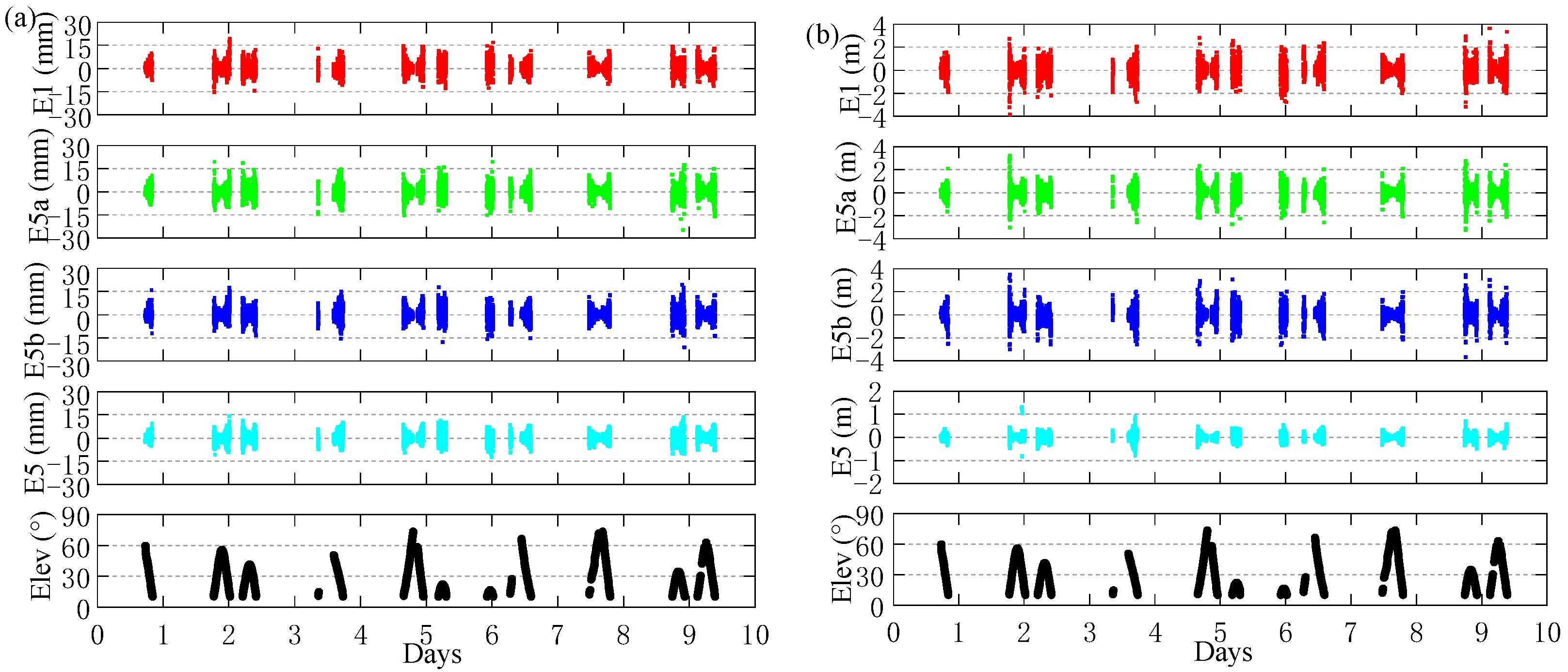
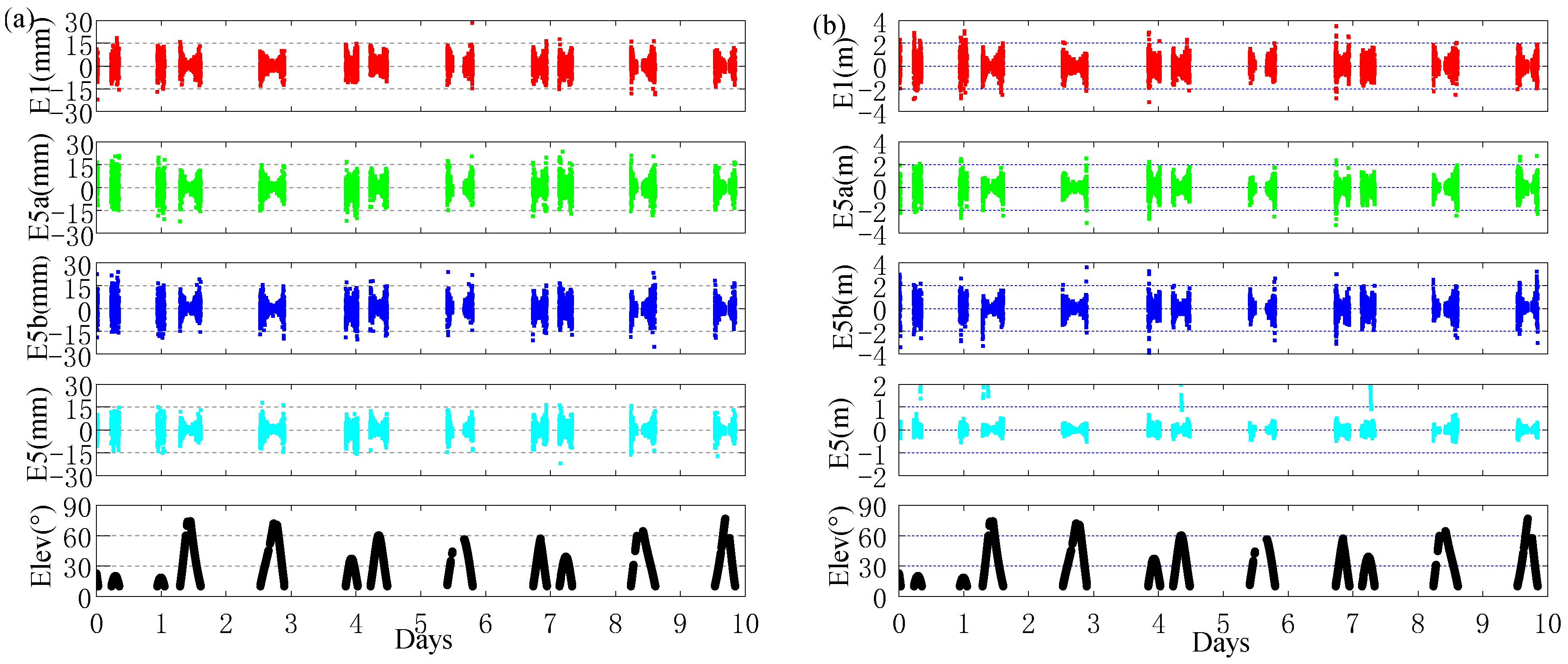
Figure 9 and Figure 10 show the time series of pseudo-range and carrier phase single-difference residuals for Galileo FOC (E03) and IOV (E19) satellites, respectively. From the figures, the single-difference carrier phase and single-difference pseudo-range residuals of Galileo are within $\pm$15 mm and 2 m, respectively. Under the influence of pseudo-range multipath and noise, the lower the cut-off elevation, the larger the single-difference residual. Based on the single-difference residuals, the statistical results of the raw pseudo-range and carrier phase accuracy are shown in

Table 3. Accuracy of pseudo-range and carrier phase observation (RMS).

	Galileo	Pseudo-Range (m)				Phase (mm)
		E1	E5a	E5b	E5	E1	E5a	E5b	E5
IOV	E11	0.385	0.319	0.373	0.428	2.412	2.811	2.616	1.990
	E12	0.367	0.307	0.352	0.297	2.321	2.635	2.545	1.915
	E19	0.426	0.373	0.418	0.234	2.837	3.325	3.715	2.474
	Average	0.393	0.333	0.381	0.319	2.523	2.924	2.959	2.126
FOC	E02	0.428	0.372	0.417	0.386	2.450	2.634	2.534	1.936
	E03	0.435	0.376	0.420	0.213	2.451	2.691	2.615	1.938
	E08	0.419	0.364	0.413	0.167	2.532	2.657	2.509	1.861
	E09	0.431	0.398	0.447	0.268	2.476	2.670	2.598	2.015
	E18	0.346	0.312	0.327	0.096	2.124	2.304	2.380	1.678
	Average	0.412	0.364	0.405	0.226	2.406	2.591	2.527	1.886

. From Table 3, Galileo quad-frequency pseudo-range observations have an accuracy of about 20~50 cm. The carrier phase observations have an accuracy of about 1~3 mm, and the accuracy of the observations at E5 is significantly better than E1, E5a, and E5b frequency. The accuracy of FOC observations is basically equivalent to IOV observations.

3.3. GB-QCAR Implementation for Galileo

The idea of the GB-QCAR method is to fix the integer ambiguity of EWL, VWL, WL, and NL combinations step and step. In each step, the least square is used to solve the floating solution of ambiguity, and the integer ambiguity is fixed by the Lambda algorithm. The ratio test is used for ambiguity fixing in this study.

In the first step, the pseudo-range observation for ${\mathit{O}}_p$ can be used together with the carrier phase combinations to fix the EWL ambiguity:

$$\left\{\begin{array}{l}\mathit{A}\mathit{X}={\mathit{O}}_P+{\epsilon }_P\\ \mathit{A}\mathit{X}+{\lambda }_{g_e,h_e,k_e,l_e}{\mathit{N}}_{g_e,h_e,k_e,l_e}={\mathit{O}}_{{\phi }_{g_e,h_e,k_e,l_e}}+{\epsilon }_{{\phi }_{g_e,h_e,k_e,l_e}}\end{array}\right.$$

(15)

where X is the position vector, A is the linear coefficient matric; The subscript $g_e,h_e,k_e,l_e$ denotes EWL. ${\mathit{O}}_{g_e,h_e,k_e,l_e}$ is the EWL combined carrier phase observation with the EWL wavelength ${\lambda }_{g_e,h_e,k_e,l_e}$; ${\epsilon }_P,{\epsilon }_{{\phi }_{g_e,h_e,k_e,l_e}}$ are the noises of pseudo-range, and EWL observations, respectively.

In the second step, we can obtain the VWL ambiguity using the fixed ambiguity EWL:

$$\left\{\begin{array}{l}\mathit{A}\mathit{X}={\mathit{O}}_{{\phi }_{g_e,h_e,k_e,l_e}}-{\lambda }_{g_e,h_e,k_e,l_e}{\mathit{N}}_{g_e,h_e,k_e,l_e}+{\epsilon }_{{\phi }_{g_e,h_e,k_e,l_e}}\\ \mathit{A}\mathit{X}+{\lambda }_{g_v,h_v,k_v,l_v}{\mathit{N}}_{g_v,h_v,k_v,l_v}={\mathit{O}}_{{\phi }_{g_v,h_v,k_v,l_v}}+{\epsilon }_{{\phi }_{g_v,h_v,k_v,l_v}}\end{array}\right.$$

(16)

where the subscript $g_v,h_v,k_v,l_v$ denotes the VWL coefficient. ${\mathit{O}}_{g_v,h_v,k_v,l_v}$ is the VWL combined carrier phase observation with the VWL wavelength ${\lambda }_{g_v,h_v,k_v,l_v}$; ${\epsilon }_{{\phi }_{g_v,h_v,k_v,l_v}}$ is the noises of the VWL observations.

In the third step, the estimation obtained above for ${\mathit{N}}_{g_v,h_v,k_v,l_v}$ can be used together with the WL carrier phase combinations to fix the WL ambiguity:

$$\left\{\begin{array}{l}\mathit{A}\mathit{X}={\mathit{O}}_{{\phi }_{g_v,h_v,k_v,l_v}}-{\lambda }_{g_v,h_v,k_v,l_v}{\mathit{N}}_{g_v,h_v,k_v,l_v}+{\epsilon }_{{\phi }_{g_v,h_v,k_v,l_v}}\\ \mathit{A}\mathit{X}+{\lambda }_{g_w,h_w,k_w,l_w}{\mathit{N}}_{g_w,h_w,k_w,l_w}={\mathit{O}}_{{\phi }_{g_w,h_w,k_w,l_w}}+{\epsilon }_{{\phi }_{g_w,h_w,k_w,l_w}}\end{array}\right.$$

(17)

where the $g_w,h_w,k_w,l_w$ denotes WL coefficient. ${\mathit{O}}_{g_w,h_w,k_w,l_w}$ is the WL combined carrier phase observation with the WL wavelength ${\lambda }_{g_w,h_w,k_w,l_w}$; ${\epsilon }_{{\phi }_{g_w,h_w,k_w,l_w}}$ is the noises of the WL observations.

In the last step, the NL ambiguity can be fixed together with the obtained WL ambiguity:

$$\left\{\begin{array}{l}\mathit{A}\mathit{X}={\mathit{O}}_{{\phi }_{g_w,h_w,k_w,l_w}}-{\lambda }_{g_w,h_w,k_w,l_w}{\mathit{N}}_{g_w,h_w,k_w,l_w}+{\epsilon }_{{\phi }_{g_w,h_w,k_w,l_w}}\\ \mathit{A}\mathit{X}+{\lambda }_{g_n,h_n,k_n,l_n}{\mathit{N}}_{g_n,h_n,k_n,l_n}={\mathit{O}}_{{\phi }_{g_n,h_n,k_n,l_n}}+{\epsilon }_{{\phi }_{g_n,h_n,k_n,l_n}}\end{array}\right.$$

(18)

where the subscript $g_n,h_n,k_n,l_n$ denotes NL. ${\mathit{O}}_{g_n,h_n,k_n,l_n}$ is the NL combined carrier phase observation with the NL wavelength ${\lambda }_{g_n,h_n,k_n,l_n}$; ${\epsilon }_{{\phi }_{g_n,h_n,k_n,l_n}}$ is the noises of the NL observations.

For the GB-QCAR method, the ambiguity ${\mathit{N}}_{g_e,h_e,k_e,l_e}$ is solved by using the pseudo-range observations combined with the longest equivalent wavelength (Equation (15)). Then we can fix ${\mathit{N}}_{g_e,h_e,k_e,l_e}$ to its integer and solve for the combination with the second longest equivalent wavelength (Equation (16)). Sequentially, we will carry on the process until the four independent ambiguities are estimated as their integers (Equations (17) and (18)).

To verify the performance of the GB-QCAR method, the data are collected from Galileo quad-frequency static observation with two baselines (Baseline A and Baseline B). It is 2 consecutive days from 17 to 18 December 2018. The lengths of the two baselines are 7.9 km and 22.4 km, respectively. The observations were collected with 30 s sampling interval.

Table 4. Characteristics of the data.

Dataset	Baseline	Length	Data	Interval (s)	Location
A	CUT0-UWA0	7.9 km	DOY 350–356, 2018	30	Curtin University, Perth, Australia
B	CUT0-PERT	22.4 km	DOY 350–356, 2018	30	Curtin University, Perth, Australia

gives the details of these two baselines.

Table 5. A list of different options for the Galileo QCAR method.

Option	EWL	VWL	WL	NL
1	(0, −1, 1, 0)	(1, 2, −4, 1)	(1, 0, 0, −1)	(1, 0, 0, 0)
2	(0, −1, 1, 0)	(0, −2, 1, 1)	(1, 0, 0, −1)	(1, 0, 0, 0)
3	(0, −1, 1, 0)	(0, −3, 2, 1)	(1, 0, 0, −1)	(1, 0, 0, 0)
4	(0, −1, 1, 0)	(0, −4, 3, 1)	(1, 0, 0, −1)	(1, 0, 0, 0)
5	(0, −1, 1, 0)	(0, −3, 5, −2)	(1, 0, 0, −1)	(1, 0, 0, 0)
6	(0, −1, 1, 0)	(1, 9, −7, −3)	(1, 0, 0, −1)	(1, 0, 0, 0)
7	(0, −1, 1, 0)	(0, −3, 5, −2)	(1, 0, 0, −1)	(0, 0, 0, 1)
8	(0, −1, 1, 0)	(0, −3, 5, −2)	(1, −1, 0, 0)	(0, 0, 0, 1)
9	(0, −1, 1, 0)	(0, −3, 5, −2)	(1, 0, −1, 0)	(0, 0, 0, 1)
10	(0, −1, 1, 0)	(0, −3, 5, −2)	(1, 0, −1, 0)	(1, 0, 0, 0)

gives ten different options for the Galileo GB-QCAR method.

Table 6. Baseline A ambiguity-fixed rate for different linear combinations (%).

Option	EWL	VWL	WL	NL
1	100	88.26	97.62	98.41
2	100	100	92.26	98.99
3	100	100	94.09	99.26
4	100	100	95.09	99.41
5	100	100	95.53	99.59
6	100	85.58	77.23	98.18
7	100	100	95.53	99.68
8	100	100	95.47	99.71
9	100	100	95.38	99.47
10	100	100	95.38	99.26

and

Table 7. Baseline B ambiguity-fixed rate for different linear combinations based (%).

Option	EWL	VWL	WL	NL
1	100	78.60	94.17	92.26
2	100	100	85.08	93.01
3	100	100	87.98	94.17
4	100	100	89.64	95.19
5	100	100	90.01	95.36
6	100	75.60	68.29	91.99
7	100	100	90.01	95.76
8	100	100	90.01	96.13
9	100	100	90.01	95.54
10	100	100	90.01	94.37

give the ambiguity-fixed rate of ten options for baseline A and B, respectively. We can conclude as follows: using the GB-QCAR method, the ambiguity-fixed rate of the basic signal reaches 90%, indicating that Galileo can perform effective positioning services. In the two baselines, the ambiguity-fixed rate of combinations EWL (0, −1, 1, 0) reaches 100%, and the ambiguity-fixed rate of VWL combinations reaches 100%, such as (0, −2, 1, 1) (0, −3, 2, 1) (0, −4, 3, 1) (0, −3, 5, −2). The ambiguity-fixed rate of Option 7 is higher than that of Option 5, mainly because the E5 signal generates composite signals from E5a and E5b, which have a longer wavelength and less noise. With the increase of baseline length, the ambiguity-fixed rate of baseline B decreases due to the effects of errors such as the ionospheric delay. The highest ambiguity-fixed rates of Option 8 ((0, −1, 1, 0), (0, −3, 5, −2), (1, −1, 0, 0), (0, 0, 0, 1)) are 99.71% and 96.13% for baselines A and B, respectively.

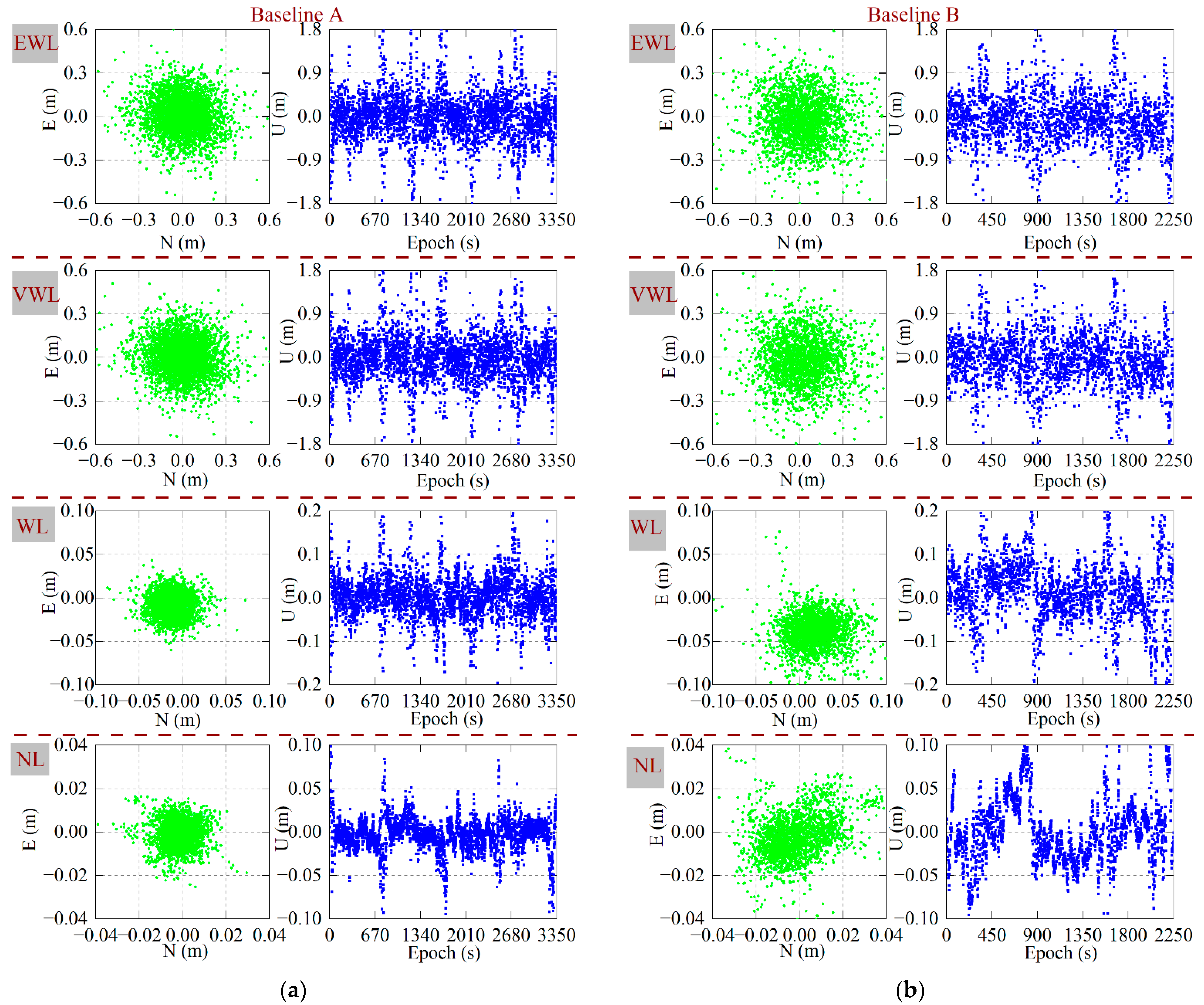
To make further efforts to analyze the positioning accuracy of the EWL, VWL, WL, and NL combinations in Option 8, Figure 11 shows the time series of N, E, U detections error of the combined observations at baseline A and B.

Table 8. Positioning accuracy of different combinations of observations (m).

Data	Component	EWL	VWL	WL	NL
A	N	0.146	0.148	0.014	0.006
	E	0.130	0.131	0.012	0.005
	U	0.491	0.499	0.047	0.019
B	N	0.187	0.191	0.023	0.013
	E	0.171	0.173	0.019	0.010
	U	0.528	0.534	0.064	0.035

summarizes the root mean square (RMS) of positioning error for different combinations observations. It can be seen from the figures that the horizontal positioning error of the EWL combined observation (0, −1, 1, 0) and VWL combined observation (0, −3, 5, −2) are less than 0.8 m, and the elevation direction are less than 2 m. The horizontal positioning error of the WL combined observation (1, −1, 0, 0) is less than 0.1 m and the elevation direction is less than 0.2 m; The horizontal positioning error of NL E5 observations is less than 0.04 m and the elevation direction is less than 0.1 m. In Table 8, we can see that the RMS of the EWL horizontal positioning error of EWL combined observation (0, −1, 1, 0) is basically 10~20 cm, and the elevation direction is about 50 cm. The RMS of the positioning error for the VWL combined observation (0, −3, 5, −2) is equivalent to that of the EWL. The RMS of the horizontal positioning error for WL combined observation (1, −1, 0, 0) is better than 3 cm, and the elevation direction is better than 10 cm. The RMS of the NL E5 observations horizontal positioning error is about 1 cm, and the elevation direction is better than 4 cm. In summary, Galileo quad-frequency observations can achieve decimeter, centimeter, and sub-centimeter positioning levels. The multi-frequency combined observations effectively improve the ambiguity-fixed rate and the reliability of positioning.

4. Discussion

The a priori precision of pseudorange and carrier depends on the observation environments and the types of receivers. Therefore, it is necessary to evaluate the Galileo observation accuracy of different types of receivers. From Table 2, Galileo quad-frequency pseudo-range observations have an accuracy of about 20~50 cm. The carrier phase observations have an accuracy of about 1~3 mm, and the accuracy of the observations at E5 is significantly better than E1, E5a, and E5b frequency.

Multi-frequency combined observation can improve the fixed rate of ambiguity [31]. Therefore, how to obtain the combined observation with low noise and long wavelength. In the article, the optimal linear combinations are selected for Galileo quad-frequency observation. Table 3 shows that the total noise from combined observations is less than 1 cycle when the first-order ionospheric error is 0.02 m.

The current research mainly focuses on the fixed rate of integer ambiguity for Galileo single frequency observations and multi-frequency non-combined observations [11,12]. Compared with single frequency or non-combined observations, the fixed rate of ambiguity of Galileo quad-frequency combined observations is improved. The highest ambiguity-fixed rates of Option 8 ((0, −1, 1, 0), (0, −3, 5, −2), (1, −1, 0, 0), (0, 0, 0, 1)) based GB-QCAR) methods are 99.71% and 96.13% for the 7.9 km and 22.4 km baselines, respectively.

5. Conclusions

It is feasible to improve the ambiguity resolution performance through various linear combinations of Galileo multi-frequency signals. First, we analyzed the carrier-to-noise (C/N0), multipath combination (MPC), and the pseudo-range and phase noise using the ultra-short baseline. Second, a list of the optimal linear combinations was selected for Galileo quad-frequency observation. Finally, a geometry-based quad-frequency carrier ambiguities (GB-QCAR) method was presented in detail, and all different options of linear combinations were analyzed systematically with respect to the ambiguity-fixed rate. According to the experimental results,

(1) For the same type of satellite, the C/N0 values of the E5 signal perform the best among all frequencies, while the E1 signal is the worst. At the same cut-off elevation angle, the C/N0 value of the FOC satellite is 3~4 dB-Hz higher than that of the IOV satellite at all signals. In terms of MPC, the RMS of MPC for Galileo signals are all less than 0.3 m, and they are ordered as E1 $\approx$ E5b > E5a > E5. Galileo quad-frequency pseudo-range observations have an accuracy of about 20~50 cm. The carrier phase observations have an accuracy of about 1~3 mm, and the accuracy of the observations at E5 is significantly better than E1, E5a, and E5b frequency. The accuracy of FOC observations is basically equivalent to IOV observations.

(2) In the 7.9 km and 22.4 km baselines, the ambiguity-fixed rate of combinations EWL (0, −1, 1, 0) reaches 100%, and the ambiguity-fixed rate of VEL combinations reaches 100%, such as (0, −2, 1, 1) (0, −3, 2, 1) (0, −4, 3, 1) (0, −3, 5, −2). Compared with Option 5 ((0, −1, 1, 0), (0, −3, 5, −2), (1, 0, 0, −1), (1, 0, 0, 0)), Option 7 ((0, −1, 1, 0), (0, −3, 5, −2), (1, 0, 0, −1), (0, 0, 0, 1)) has a higher ambiguity-fixed rate, mainly because the E5 signal has a longer wavelength and less noise. With the increases in the baseline, the ambiguity-fixed rate of 22.4 km baseline decreases, due to the effects of errors such as the ionospheric delay. The highest ambiguity-fixed rates of Option 8 ((0, −1, 1, 0), (0, −3, 5, −2), (1, −1, 0, 0), (0, 0, 0, 1)) are 99.71% and 96.13% for the 7.9 km and 22.4 km baselines, respectively.

(3) The RMS of horizontal positioning error for the EWL combined observation (0, −1, 1, 0) is basically 10~20 cm, and the elevation direction is about 50 cm. The RMS of the positioning error for the VWL combined observation (0, −3, 5, −2) is equivalent to that of the EWL. The RMS of the horizontal positioning error for WL combined observation (1, −1, 0, 0) is less than 3 cm, and the elevation direction is less than 10 cm. The RMS of the horizontal positioning error of the NL E5 observations is about 1 cm, and the elevation direction is less than 4 cm. In summary, Galileo quad-frequency observations can achieve decimeter, centimeter, and sub-centimeter positioning levels, which improve the ambiguity-fixed rate and the reliability of positioning.