An Integrated Quantitative Method Based on ArcGIS Evaluating the Contribution of Rural Straw Open Burning to Urban Fine Particulate Pollution

Abstract

This study presents a GIS-based method integrating hourly transport pathways and wind-field grid reconstruction, straw open burning (SOB) source identification, and a two-stage spatiotemporal multi-box modeling approach to quantify the contribution of external sources of SOB to elevated urban PM_2.5 concentrations during a specific pollution episode (PE) at a high temporal resolution of 1 h. Taking Jilin Province as an empirical study, the contribution of SOB in province-wide farmlands to urban haze episodes in Changchun during the SOB season of 2020–2021 was evaluated quantitatively using a combination of multi-source datasets. The results showed that Changchun experienced three severe PEs and one heavy PE during the study period, and the total PM_2.5 contributions from SOB sources were 352 μg m⁻³, 872 μg m⁻³, and 1224 μg m⁻³ during the three severe PEs, respectively; these accounted for 7%, 27%, and 23% of the urban cumulative PM_2.5 levels, which were more obvious than the contribution during the PE. The total PM_2.5 contribution from SOB sources (4.9 μg m⁻³) was only 0.31% of the urban cumulative PM_2.5 level during the heavy PE. According to the analysis of the impact of individual factors, some policy suggestions are put forward for refined SOB management, including control spatial scope, burning time interval, as well as burning area limit under different urban and transport pathways’ meteorological conditions and different transport distances.

1. Introduction

Urban particulate pollution episodes (PEs) are usually attributed to not only local emissions related to the levels of urbanization and industrialization, but also the regional or even trans-boundary transport of polluted air masses from external source areas [1,2]. Especially for cities located in major grain-producing areas of China, straw open burning (SOB) in the farmlands of rural areas has been identified as among the largest regional sources that can significantly affect urban air quality and result in haze episodes [3,4,5]. When biomass burning occurs, a large number of particulates are produced and released into the atmosphere in a short time with uncontrolled combustion [6,7]. Then, air parcels can carry the particulate matter to downwind urban areas through atmospheric transport and circulation [8,9]. Intense straw burning has attracted widespread attention due to its catastrophic fine particulate matter (PM_2.5) pollution and its threats to inhabitants’ health [10,11,12].

Although a strict prohibition policy of unauthorized or unordered straw burning has been adopted by the government, owing to high straw yield and the limitation of the high cost of collecting and transporting, it is difficult to rapidly improve the capacity of straw utilization for resources and to completely consume all crop residues within a short time; a considerable amount of straw is still discarded and has to be burned to prepare for planting in the coming spring. Consequently, in order to minimize the impact of SOB on the air quality of urban areas under the premise of ensuring agricultural production and food security, it is essential to burn the discarded straw in a planned and systematic manner, which can further eliminate the conflict between environmental management enforcers and farmers. Therefore, quantitative assessment of the regional transport of straw burning-sourced PM_2.5 in rural areas and its contribution to urban haze episodes has significance for implementing targeted emission-control measures.

Several methods have been applied to estimate the impacts of external particulate sources on local air quality. Backward trajectory analysis is one of the most commonly used methods for analyzing pollution episodes and tracing the historical location of air masses passing over to identify their potential external sources. Backward trajectory modeling, combined with atmospheric concentrations at the receptor site, generally includes the potential source contribution function (PSCF) [13,14], gridded frequency distributions (GFD) [15], concentration-field analysis, concentration-weighted trajectory (CWT) [16], trajectory clustering analysis, residence-time-weighted concentration (RTWC) [13,17], and conditional probability function (CPF) [18]. All these models are essentially statistical analyses of many (over months to years) trajectories by counting the frequency of back-trajectory segment endpoints in grid cells to show the geographic origin most associated with elevated concentrations among long-term air pollution measurement data [19]. However, they cannot quantify the regional transport mass or concentration of PM_2.5.

Another commonly used approach is based on air quality models such as WRF-CMAQ, WRF-CAMx, and WRF-CHEM, including sensitivity analysis [20,21,22] and transport flux approaches [23,24,25], among others [26,27,28]. The characteristics of the transport pollutant and its contribution to high particulate pollution can be quantified using computational atmospheric models. However, the sensitivity of PM_2.5 concentration in the receptor city to emissions from the source area is not necessarily the same as the contribution of transport, due to the non-linear relationships between emissions and concentrations [29]. A transport flux approach is usually applied to assess the large-scale transport of air pollutants, such as inter-continental and trans-boundary [30,31,32]. These approaches, based on air quality models, are effective only in the context of accurate emission inventories, reliable weather simulations, and comprehensive descriptions of chemical reactions since they are based on the simulated meteorology field and air pollutant concentrations.

Despite the preceding methods, the quantity of external sources of straw burning in rural areas and the duration of burning may affect urban air quality, and have rarely been assessed quantitatively and systematically; our understanding of the influence of burning area, transport distance, and meteorological conditions along transport pathways are neither complete nor comprehensive. This is because it is difficult to identify the potential spatial scope of external straw burning sites associated with elevated PM_2.5 concentrations of the receptor city with a high temporal resolution, such as during ten to dozens of hours of a specific haze episode. The geographic origin, identified using trajectory statistical methods, is the probability that an external source is located at a point location with latitude and longitude, rather than the exact spatial scope. This is semi-quantitative, which is suitable for identifying long-term transport characteristics. For methods based on air quality models, the subdomains of emission scenarios should be arranged in advance, and the results should be limited to the pre-divided subdomains. However, straw burning associated with a specific haze episode of a receptor city is rather sporadic and transient [33], it may occur randomly anywhere on farmland in a rural area surrounding a city, and a single burning lasts only a few hours.

This study constructs a GIS-based integrated method including multiple techniques and models with collaborative multi-source datasets to quantify the contribution of external SOB sources to the elevated urban PM_2.5 concentrations during specific haze episodes. The integrated model offers the possibility to link the spatial scope of external SOB sources, their transport pathways, and the pollution level of the receptor city at a high temporal resolution (1 h). Taking Jilin Province as the study area, and its capital Changchun as the pollution receptor city, SOB in province-wide farmland is examined, and its contribution to specific urban haze episodes during the SOB season of 2020–2021 is assessed quantitatively. Moreover, the impact of the area of SOB sources, their transport distance, average planetary boundary layer height (PBLH) along the transport pathway, urban PBLH, and urban wind speed are explored. The results will be beneficial to policymakers in developing refined management regulations on SOB to protect the atmospheric environment and to ensure agricultural production as well.

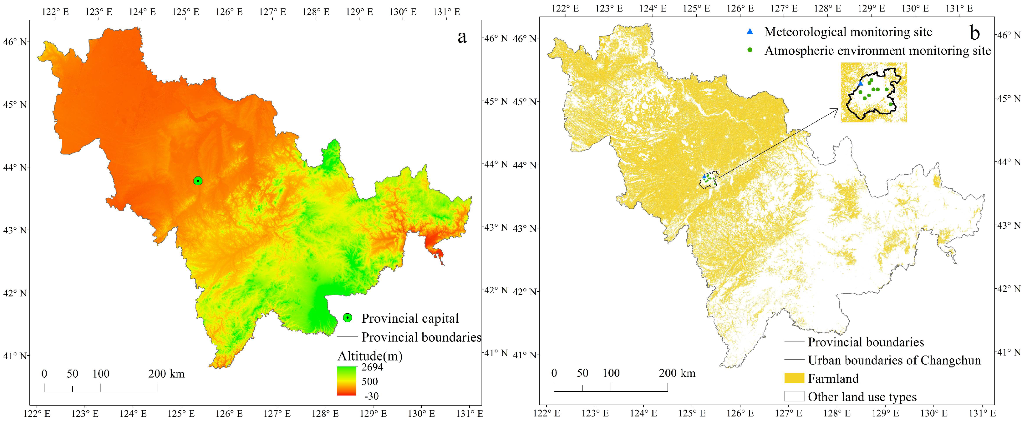
2. Overview of Study Area and Period

Jilin Province is located in Northeast China with a population of 25.77 million and comprises an area of 191,341 km²; it is one of the most important agricultural provinces of China. The farmland is mainly distributed in the central and western plains as shown in Figure 1. The area is 7.4985 million hm², of which 5.6818 million hm² consists of grain crops that yielded 38.03 million tons in 2020 [34]. At present, a considerable amount of crop residue is still discarded on the farmland during the fallow season because of the high cost of collection and transportation, although a portion is recycled as fertilizer, feed, or fuel. Jilin Province is located in a mid-temperate zone, the crops are harvested once a year in October, and soil tillage and crop planting for the next crop starts in May. The farmland is often covered with snow over the winter, which is not conducive to biomass burning. Therefore, SOB in Jilin Province has obvious seasonal characteristics and mostly takes place in two periods: one after fall harvesting and before the snow season, mainly in November, and the other after the snow melt in the fields and before spring plowing, mainly in April. The study period of this paper is the SOB season of 2020–2021, that is, in November 2020 and April 2021.

Changchun, the capital and the largest city of Jilin Province, is located in the middle of the province. The population in the municipal district is 4.47 million, accounting for more than 17% of the province’s total population, making it the most densely populated city in Jilin province. The urban area is surrounded by extensive farmland in the whole province, as shown in Figure 1. The surrounding farmland belongs to the black soil area of Northeast China, with high grain yield and straw density. Compared with other months of the year, the frequency of urban air quality in Changchun exceeding standards is higher during the SOB season [35,36].

3. Methodology and Data Sources

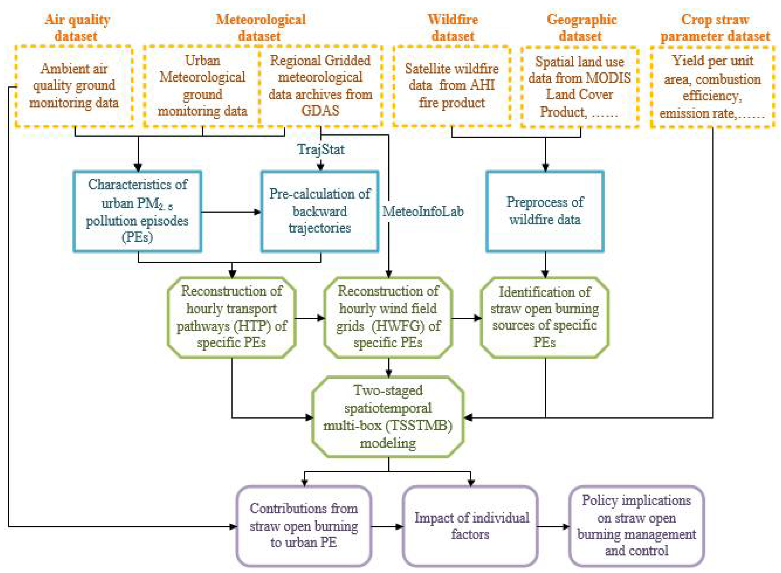
3.1. Modeling Framework

The basic framework and procedures for the GIS-based integrated method are illustrated in Figure 2. First, the frequency and characteristics of urban pollution episodes in Changchun during the SOB season of 2020–2021 were determined based on hourly air quality and meteorological data. Then, hourly transport pathways and wind-field grids of the external pollution sources during pollution episodes were reconstructed using the regional gridded meteorological data archives from the National Centers for Environmental Prediction (NCEP) Global Data Assimilation System (GDAS). Third, the preprocessed satellite wildfire data on the spatial distribution of farmlands were screened by hourly wind-field grids to identify external SOB pollution sources. Fourth, a two-stage spatiotemporal multi-box based on hourly wind-field grids was developed to estimate the contribution of external SOB pollution sources to urban pollution episodes. Finally, we analyzed the impact of individual factors, including the burning area of SOB sources, their transport distance, the average PBLH along the transport pathway, urban PBLH, and urban wind speed.

3.2. Determination of Pollution Episodes

PM_2.5 is a typical indicator of SOB-induced haze pollution episodes. In this study, PM_2.5 air pollution episodes (PEs) are defined as a consecutive duration of >10 h with the hourly average PM_2.5 concentration exceeding the Grade II China Ambient Air Quality Standard (GB3095–2012) of 75 μg m⁻³. The hourly average PM_2.5 concentrations of Changchun were obtained from the Jilin Provincial Environmental Monitoring Centre, which collects official data from all state-controlled ambient air quality ground-monitoring stations in urban areas of Changchun. The ground-monitoring data for the hourly meteorological conditions, including mean wind speed (m/s), wind direction (°), and mean relative humidity (%), were obtained from the Jilin Provincial Meteorological Service. PBLH data were from regional gridded meteorological data archives from GDAS with a resolution of 1° × 1°, which was obtained from the NOAA site [37]. Hourly PBLH was obtained via interpolation from observed data at 3 h intervals.

3.3. Reconstruction of Hourly Transport Pathways and Wind-Field Grids

The spatiotemporal distribution of hourly transport pathways and wind-field grids were reconstructed using TrajStat combined with ArcGIS software. First, air mass backward trajectories were calculated using the Hybrid Single Particle Lagrangian Integrated Trajectory (HYSPLIT-4) model [38] loaded into TrajStat, which is a GIS-based software, and we converted the backward trajectory data to ESRI “PolylineZ” shape file format [39,40]. The calculation is described in detail in Section 3.3.1. Second, the backward trajectory data in shape file format were added into ESRI ArcGIS software and we performed a series of processing steps, as elaborated in Section 3.3.2, to obtain the hourly transport pathways and wind-field grids during PEs.

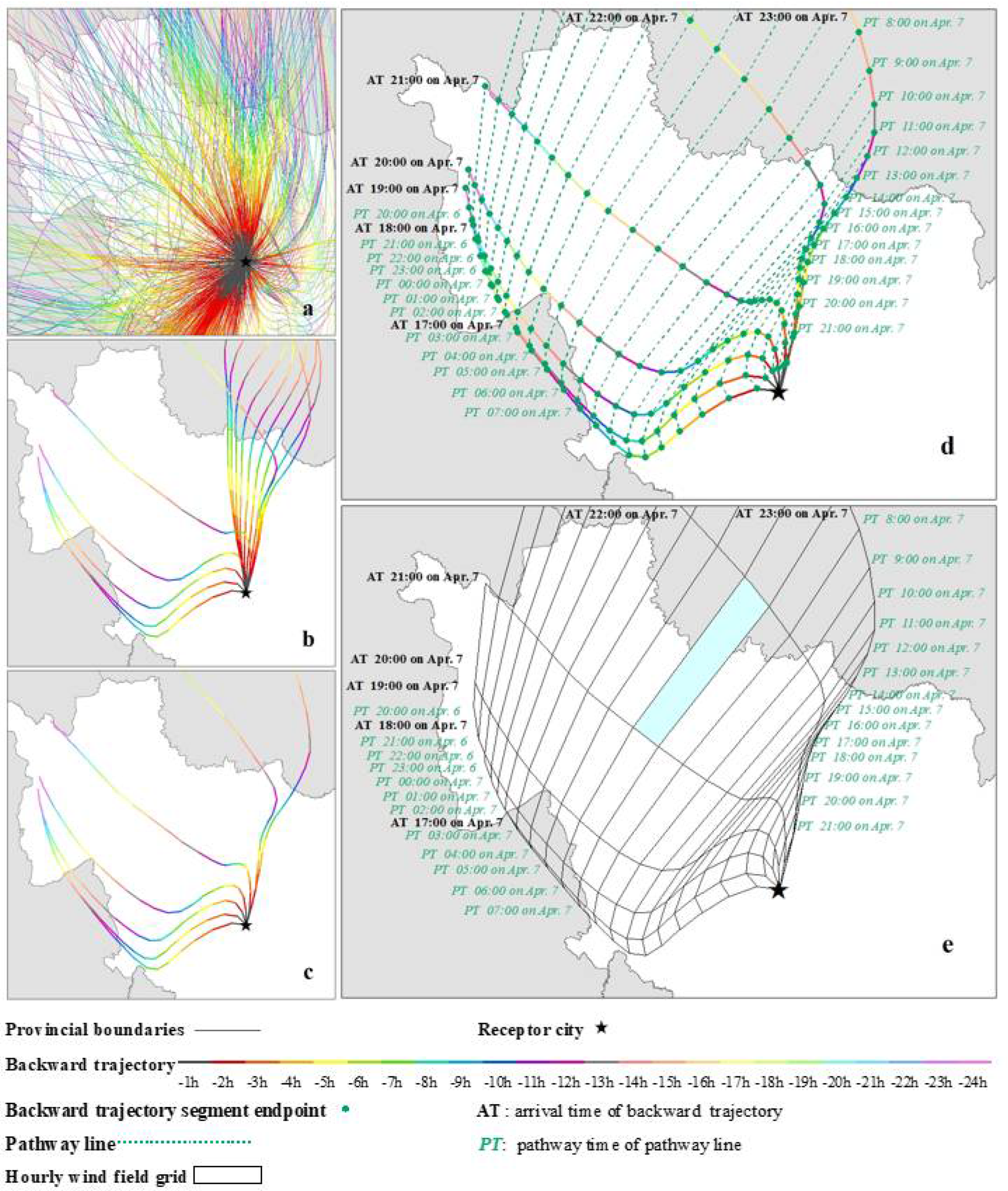
3.3.1. Pre-Calculating Backward Trajectories

The calculations of TrajStat run in units of a month, and the output trajectory data are stored in monthly files. Therefore, we pre-calculated the backward trajectories for November 2020 and April 2021, in which hourly backward trajectories with running hours from −1 h to −24 h were calculated once, and the arrival time (starting hours) of the backward trajectories were hourly intervals of a day from 0:00 to 23:00 local standard time. We used the center point of state-controlled air sampling sites in Changchun as the receptor site (start location) with an air mass arriving height of 100 m above ground level. The archived meteorological data used to calculate trajectories were GDAS with a resolution of 1° × 1°. According to the pre-research on the temporal distribution of province-wide SOB fire spots before and during each PE, the duration of continuous SOB is generally not more than 24 h before the beginning of a PE. Some studies have estimated the lifetime of atmospheric particulate matter [41,42]. Therefore, a −24 h backward trajectory will cover the potential external source areas that are likely to affect the pollution level of a specific PE.

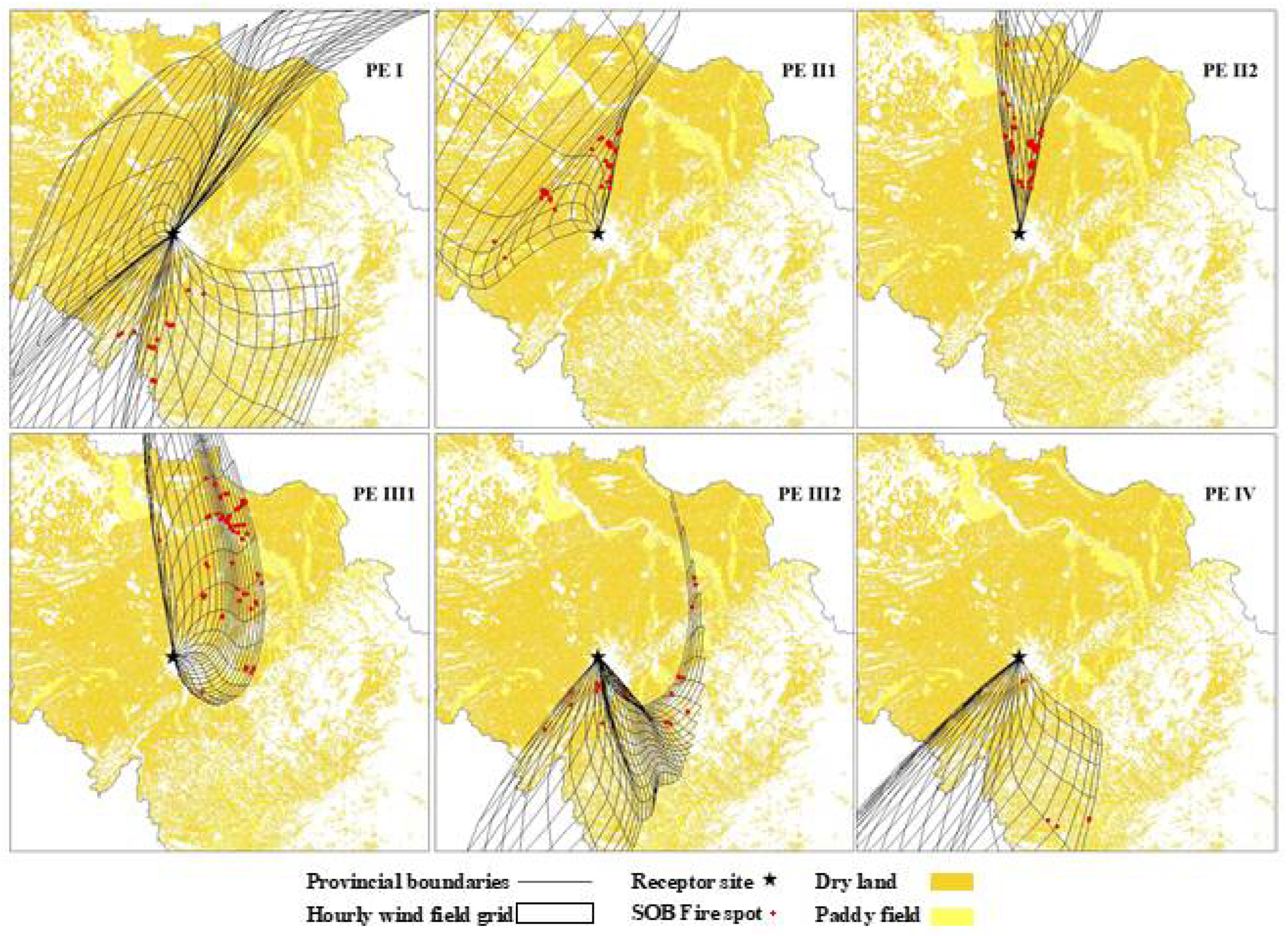
3.3.2. Plotting Hourly Transport Pathways and Wind-Field Grids

Referring to the infinite-division idea of differentiation in mathematics, there are countless suppositional trajectories with short intervals of arrival time, evenly distributed between two backward trajectories of 1 h intervals of arrival time, calculated using TrajStat. If an emission source is located in the zone between two adjacent backward trajectories of 1 h intervals of arrival time, an air parcel passing through that zone indicates that particulate matter from the source is likely to be collected and transported along the trajectory to the receptor city and contributes to the corresponding hourly average pollutant concentrations of the city. In this study, the zone between two adjacent backward trajectories of 1 h intervals of arrival time is defined as an hourly transport pathway (HTP), which shows the geographic origin of regional sources most associated with hourly average concentrations of the receptor city.

Then, we gridded the HTP and calculated the time when the air mass passed a specific grid to determine the spatiotemporal distribution of the wind field during the PE. The required steps for plotting the hourly wind-field grid (HWFG) are as follows:

(1) Pre-processing trajectory data: As mentioned previously, the back-trajectory data have an attribute column representing the arrival time of the air mass. Hourly backward trajectories whose arrival times were in accordance with the time of the PEs were selected by attribute from the monthly backward trajectory file. Taking PE II in Section 4 as an example, hourly backward trajectories with hourly arrival times from 17:00 on 7 April to 7:00 on 8 April (Figure 3b) were selected from the April 2021 backward trajectory data (Figure 3a).

(2) Reconstructing HTPs: To avoid spatial overlap, the trajectories were divided into several groups, which were calculated in the same way in the subsequent process and are shown in separate panels. The trajectories in Figure 3c, whose arrival time is from 17:00 to 23:00 on 7 April, is one of the groups during PE II, denoted as PE II1. The zone between the two adjacent backward trajectories is the HTP. For example, the zone between the backward trajectories with the arrival time of 20:00 on 7 April and 21:00 on 7 April in Figure 3c is an HTP, and it is the geographic area most strongly associated with the regional sources and which contributed to the hourly average concentration from 20:00 to 21:00 on 7 April in Changchun.

(3) Calculating pathway time and estimating the pathway line: According to the arrival time and backward hours of each trajectory, the time of each backward trajectory segment endpoint can be calculated, and it is defined as the pathway time. We connected the segment endpoints with the same pathway time to obtain a line (Figure 3d), which is defined as a pathway line indicating the geographic position of a moving air mass at the same moment as the pathway time.

(4) Reconstructing HWFGs: The grids intersected by backward trajectories and the pathway lines are the spatiotemporal distribution of the wind field (Figure 3e). For a single grid of the wind field, there are two arrival times (AT m:00 and AT n:00) of two backward trajectories and two pathway times (PT p:00 and PT q:00) of two pathway lines; these indicate the spatial distribution at p:00–q:00 of the air mass arriving at receptor site at m:00–n:00. For example, the air mass arriving at Changchun at 21:00–22:00 on 7 April 2021 was distributed in the region of the blue grid (in Figure 3e) at 6:00–7:00 on 7 April 2021.

3.4. Identification of Straw Open Burning Sources

3.4.1. Preprocessing Wildfire Data

The satellite wildfire data were extracted via the spatial distribution of farmland to screen the fire spots caused by SOB. That is, the fire spots located on farmland were identified as SOB sources, and other types of biomass burning and abnormal thermal emissions, such as forest fires and industry, were excluded.

Near-real-time wildfire data were obtained from a Himawari-8 Advanced Himawari Imager (AHI) fire product [43]. The AHI has a high temporal resolution of 10 min and a spatial resolution of 2 km. The wildfire data include the geographical location (latitude and longitude), acquisition time, hotspot intensity, and hotspot area of the fire spots, which were used to detect the spatiotemporal distribution and burning area of wildfires in different geographical regions. Wildfire data with confidence levels > 85% were used. It should be noted that to avoid repetitive statistics of hourly fire occurrence, we only counted once the Himawari-8 fires were in the same location and over continuous time within one hour. The distribution of the farmland of Jilin was identified using the MODIS Land Cover Product (MCD12Q1) at a spatial resolution of 500 m [44].

3.4.2. Identifying Potential Straw Open Burning Sources

As SOB fire spots are not fixed and are continuous emission sources, the burning time, geographical location, and burning area are random and uncertain. If SOB occurs after the air mass has passed, its contribution to the corresponding urban hourly average concentration is limited, even if the burning site is distributed in HTP reconstructed by backward trajectories. Therefore, to identify the potential SOB sources during a specific urban PE among numerous fire spots of several days or more, first, spatial overlay analysis was performed on SOB fire spots and on the HWFGs of the specific PE. Then, the acquisition time of each fire spot within the HWFGs was compared with the pathway time of the grid where it was located. According to the actual situations of Jilin Province and the questionnaire results of local farmers [45,46], the average burning time of an SOB event is three hours during the post-harvest season; we assume that the fire could last three hours prior to its detection by Himawari sensors. Therefore, a fire spot whose acquisition time is within three hours before the pathway time of its located grid is screened and identified as a potential source of the specific PE. Taking PE II1 in Section 4 as an example once again, the procedure for identifying the potential SOB sources of PE II1 is shown in Figure S1.

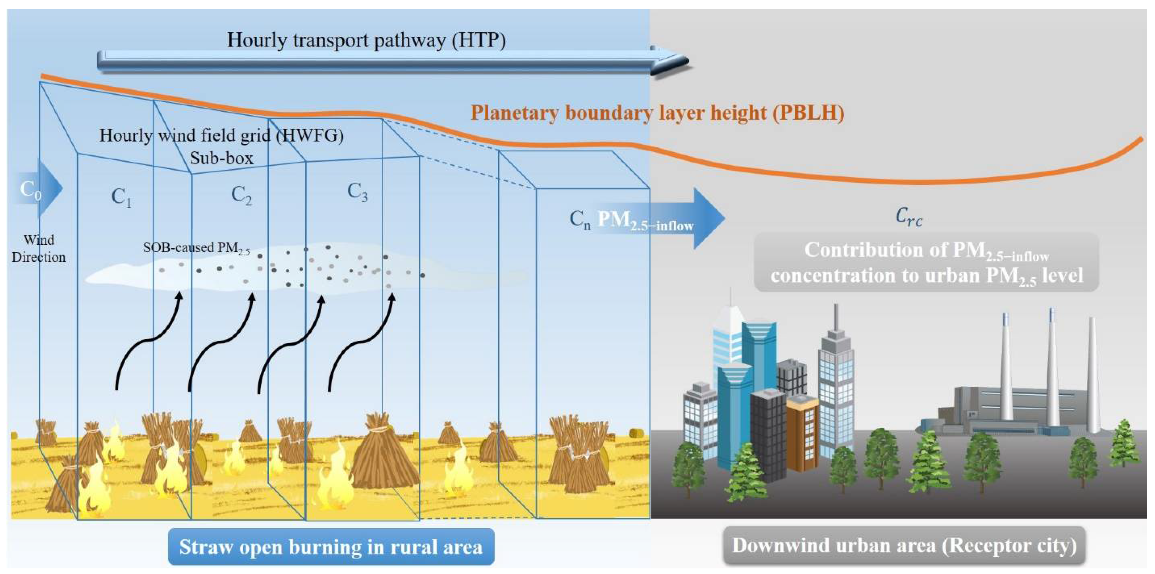
3.5. Model Formulation

Two-stage spatiotemporal multi-box (TSSTMB) modeling takes HTP as the calculation unit and treats the HWFGs and the receptor city as sub-boxes with a certain height, as shown in Figure 4. The plane size of the boxes is the area of the grids or city, and the height of the boxes is the PBLH when the air mass passes through the grids or city. The sub-boxes of the HWFGs are numbered as i (i = 1, 2, …, n, in order, far from to near the receptor city), and the receptor city sub-box is numbered as rc.

The inflow concentration of SOB-caused PM_2.5, that is, the PM_2.5 concentration of the air mass carrying SOB-caused PM_2.5 before entering the receptor city after long-range transport, was estimated in the first stage. For simplicity, the SOB-caused inflow PM_2.5 concentration into the receptor city mentioned below is denoted as PM_2.5-inflow concentration. In the second stage, the contribution of PM_2.5-inflow concentration to the urban hourly average PM_2.5 concentration was estimated.

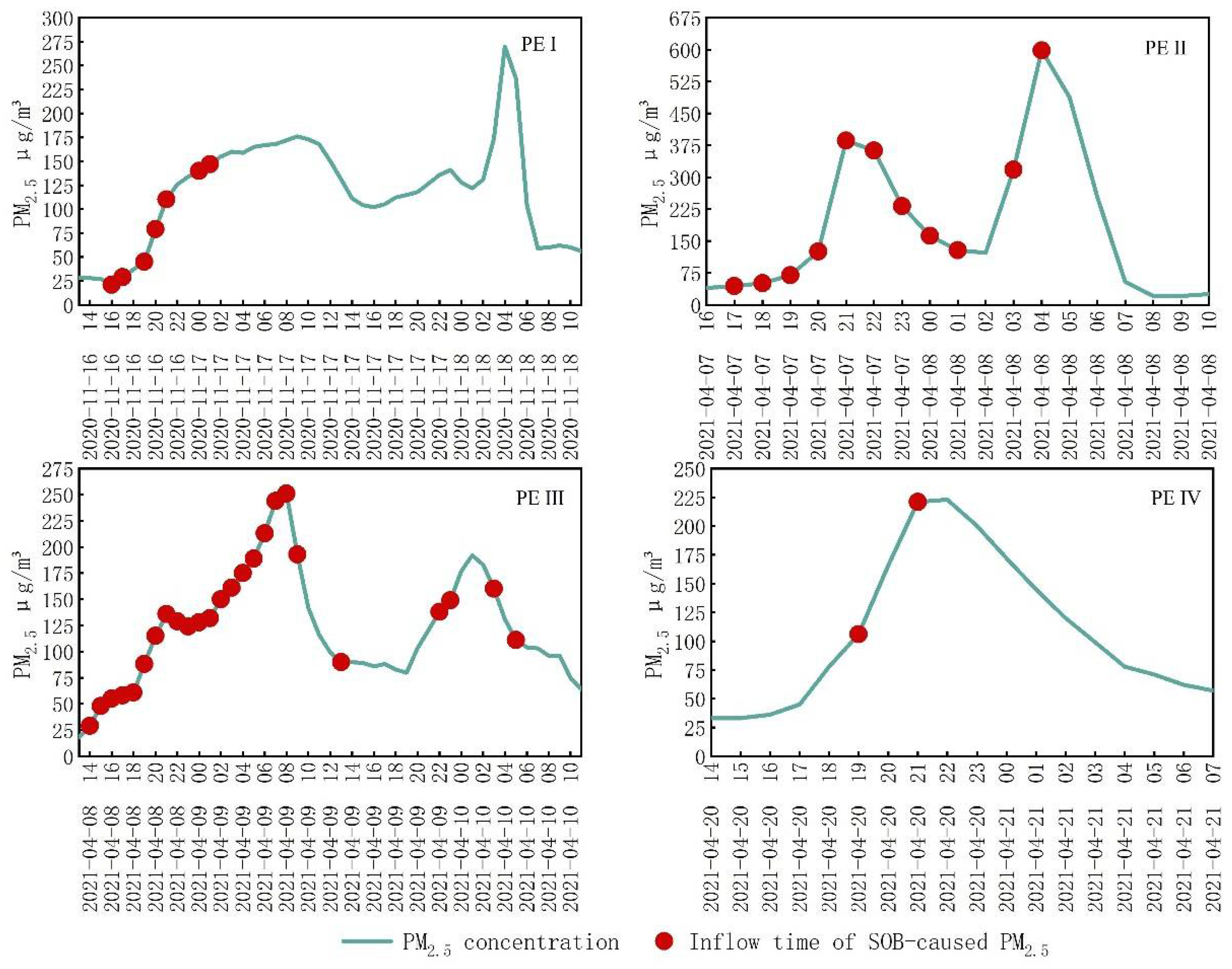
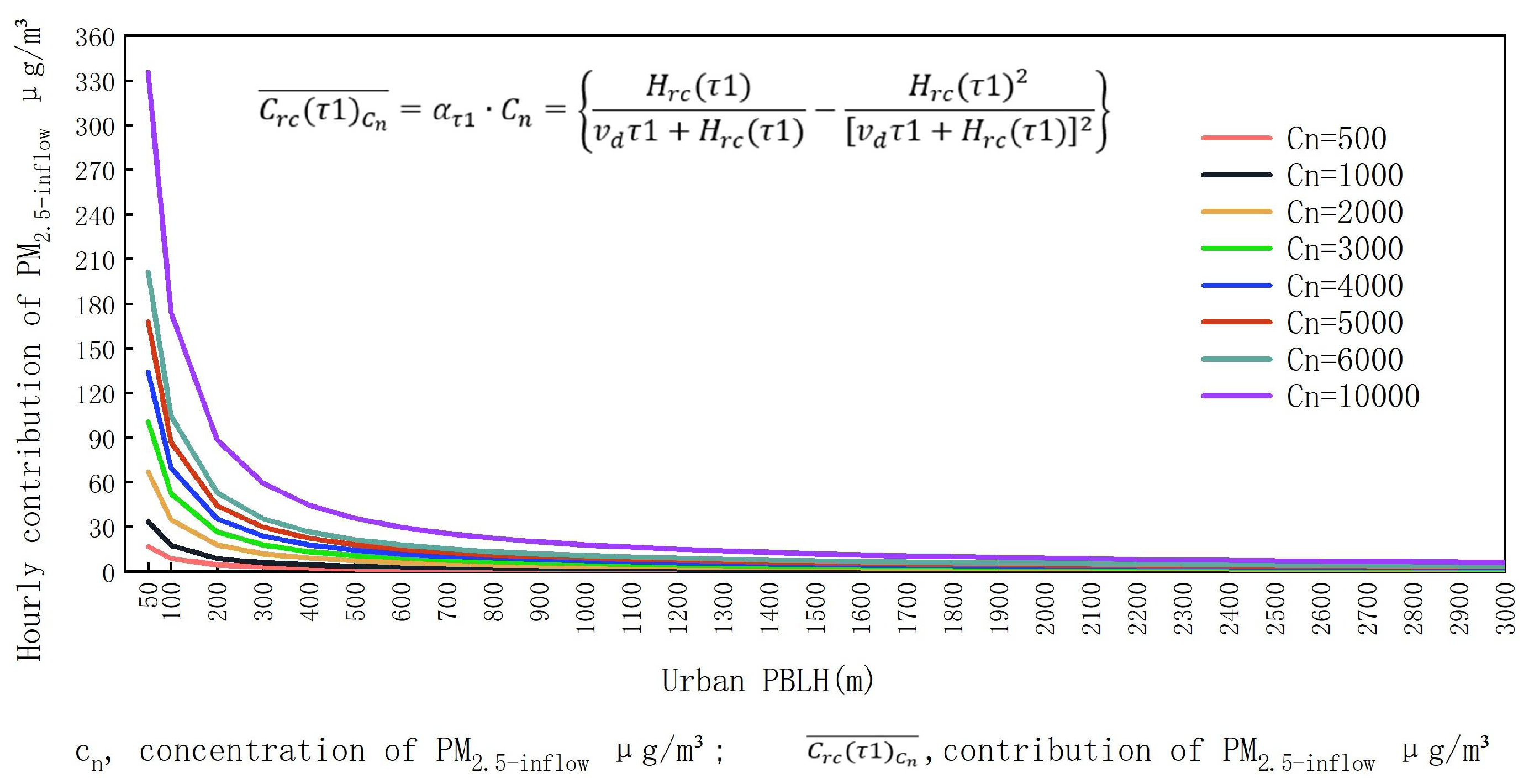
3.5.1. Estimating SOB-Caused Inflow PM_2.5 Concentration

By examining the interrelationships among the sub-boxes of HWFGs, the mass balance equation of the change in total PM_2.5 suspended in the atmosphere per unit of time in each sub-box ($∆M_i$) is established as follows:

$$∆M_i=M_i^{\mathit{Emis}}+M_i^{\mathit{Chem}}-M_i^{\mathit{Depo}}+M_i^{\mathit{Trans}}$$

(1)

where the terms on the right side of Equation (1) stand for the primary emission ($M_i^{\mathit{Emis}}$), chemical reaction ($M_i^{\mathit{Chem}}$), deposition ($M_i^{\mathit{Depo}}$), and horizontal transport ($M_i^{\mathit{Trans}}$) mass of PM_2.5 per unit of time.

The model assumes that the pollutant is completely mixed in each sub-box and pollutant concentration is uniform in the whole volume of air, so the change in total PM_2.5 per unit of time in sub-box i can be expressed as:

$$∆M_i=\frac{∆C_i}{∆t}· S_i{H}_i$$

(2)

where $∆C_i$ is the change in average PM_2.5 concentration in sub-box i (μg/m³); $S_i$ is the plane size of the sub-box; $H_i$ is the height of the sub-box and is obtained by averaging the PBLH of the four endpoints at the top of the sub-box; and ∆t is a specified period (s).

The PM_2.5 primary emission of SOB per unit of time can be described from the equation below:

$$M_i^{\mathit{Emis}}{=S}_i^c{Y}_i^c{ \rho }^c{\eta }^c{\delta }^c{q}^c+S_i^r{Y}_i^r{ \rho }^r{\eta }^r{\delta }^r{q}^r$$

(3)

where $S_i^c$ is the corn straw burning area in sub-box i (ha); $Y_i^c$ is the corn yield per unit area in sub-box i (kg/ha); ρ^c is the corn straw-to-grain ratio (%); η^c is the combustion efficiency of corn straw (%); δ^c is the dry matter rate of corn straw (%); q^c is the average PM_2.5 emission rate of burning corn straw (μg/(kg·s)); $S_i^r$ is the rice straw burning area in sub-box i (ha); $Y_i^r$ is the rice yield per unit area in sub-box i (kg/ha); ρ^r is the rice straw-to-grain ratio (%); η^r is the combustion efficiency of rice straw (%); δ^r is the dry matter rate of rice straw (%); and q^r is the average PM_2.5 emission rate of burning rice straw (μg/(kg·s)).

For particulates, both wet deposition and dry deposition are major removal mechanisms. Because there was little precipitation along the HTPs during PEs according to the prepared meteorological data, dry deposition was the main factor in removing particulate matter during the study period. The PM_2.5 deposition rate is given by

$$M_i^{\mathit{Depo}}{=C}_i · S_i{v}_d$$

(4)

where $C_i$ is the average PM_2.5 concentration in sub-box i (μg/m³) and v_d is the PM_2.5 dry deposition rate in the atmosphere (m/s).

The model assumes that advection is dominant along the wind direction, and turbulent dispersion is negligible along the wind direction and in vertical and crosswind directions. So, the PM_2.5 horizontal transport mass along the wind direction per unit of time is written as:

$$M_i^{\mathit{Trans}} {=C}_{i-1} ·{ u}_{i-1}{b}_{i-1}{h}_{i-1}-{ C}_i ·{ u}_i{b}_i{h}_i$$

(5)

where $C_{i-1}$ is the inflow PM_2.5 concentration into sub-box i, that is, the average PM_2.5 concentration in sub-box i − 1 (μg/m³); u_i−1 is the wind speed at the upwind cross-section of sub-box i, that is, wind speed at the downwind cross-section of sub-box i − 1 (m/s); b_i−1 and h_i−1 are the width and height, respectively, of the upwind cross-section of sub-box i, that is, the width and height of the downwind cross-section of sub-box i − 1 (m); u_i is the wind speed at the downwind cross-section of sub-box i (m/s); and b_i and h_i are the width and height of the downwind cross-section of sub-box i (m).

Compared with primary emissions and horizontal transport, chemical reactions within 1 h in the sub-boxes could be negligible. Therefore, after bringing in Equations (2)–(5), Equation (1) can be rewritten and converted to a differential form as follows:

$$\frac{{\mathrm{d}C}_i}{\mathrm{d}t}=\frac{S_i^c{Y}_i^c{\rho }^c{\eta }^c{\delta }^c{q}^c+S_i^r{Y}_i^r{\rho }^r{\eta }^r{\delta }^r{q}^r}{S_i{H}_i}-\frac{v_d}{H_i}{C}_i+\frac{u_{i-1}{b}_{i-1}{h}_{i-1}}{S_i{H}_i}{C}_{i-1}-\frac{u_i{b}_i{h}_i}{S_i{H}_i}{C}_i$$

(6)

As the model is based on HWFGs, the residence time for air parcels moving across sub-box i is 1 h (t = 3600 s). We assume that the air mass flowing into the first box is clean (C₀ = 0 μg/m³). Thus, in a given initial condition of ${\left.C_i\left(t\right)\right|}_{t=0}=C_i\left(0\right)$, the average PM_2.5 concentration in each sub-box C₁, C₂,…, C_n can be calculated in sequence by Equation (6). C_n, the average PM_2.5 concentration of the sub-box closest to the receptor city, is the PM_2.5-inflow concentration.

3.5.2. Evaluating the Contribution of SOB-Caused Inflow PM_2.5 Concentration

Similar to the above mass balance equation, the differential equation of the average PM_2.5 concentration in the receptor city sub-box can also be obtained as follows [47]:

$$\frac{{\mathrm{d}C}_{\mathit{rc}}}{\mathrm{d}t}=\frac{q_{\mathit{rc}}}{H_{\mathit{rc}}}+R_{\mathit{rc}}-\frac{v_d}{H_{\mathit{rc}}}{C}_{\mathit{rc}}+\frac{1}{T}\left(C_n-C_{\mathit{rc}}\right)$$

(7)

The terms on the right-hand side of Equation (7) stand for changes in PM_2.5 concentration due to local emissions, chemical reactions, deposition, and horizontal transport. C_rc, q_rc, R_rc, H_rc, and u_rc are, respectively, the average PM_2.5 concentration, local PM_2.5 emission rate, PM_2.5 chemical reaction rate, PBLH, and wind speed of the receptor city. According to the average 25 km diameter of the urban geographic space of the receptor city Changchun, it can be estimated that the residence time of the air mass is generally greater than 1 h at normal wind speeds. Therefore, when simulating the hourly average PM_2.5 concentration of the city, T is the moving time in the recipient city of the air mass with the PM_2.5-inflow concentration.

Subjected to a given initial condition, ${\left.C_{rc}\left(t\right)\right|}_{t=0}=C_{rc}\left(0\right)$, the hourly average PM_2.5 concentrations of the receptor city ($\overline{C_{rc}}$) predicted by the box model can be written as:

$$\begin{gathered} \overline{C_{rc}}=\frac{1}{T}{{\displaystyle \int }}_0^T\left[ \frac{A}{B}\left(1-e^{-\mathit{Bt}} \right)+C_{rc}\left(0\right)e^{-\mathit{Bt}} \right]\mathrm{d}t \\ =\frac{A}{B}+\frac{e^{-\mathit{BT}}-1}{T}\left(\frac{A}{B^2}-\frac{C_{rc}\left(0\right)}{B}\right) \end{gathered}$$

(8)

with

$$A=\frac{q_{\mathit{rc}}}{H_{\mathit{rc}}}+R_{\mathit{rc}}+\frac{C_n}{T}$$

$$B=\frac{v_d}{H_{\mathit{rc}}}+\frac{1}{T}$$

The solution of Equation (8) is obtained for the hourly average PM_2.5 concentration of the receptor city:

$$\begin{gathered} \overline{C_{rc}}=\left[\frac{1}{v_d+\frac{H_{\mathit{rc}}}{T}}-\frac{1}{{\mathit{TH}}_{\mathit{rc}}{\left(\frac{v_d}{H_{\mathit{rc}}}+\frac{1}{T}\right)}^2}\right]q_{\mathit{rc}}+ \\ \left[\frac{1}{\frac{v_d}{H_{\mathit{rc}}}+\frac{1}{T}}-\frac{1}{T{\left(\frac{v_d}{H_{\mathit{rc}}}+\frac{1}{T}\right)}^2}\right]R_{\mathit{rc}}+ \\ \left[\frac{1}{\frac{v_{d}T}{H_{\mathit{rc}}}+1}-\frac{1}{T^2{\left(\frac{v_d}{H_{\mathit{rc}}}+\frac{1}{T}\right)}^2}\right]C_n+ \\ \frac{1}{T\left(\frac{v_d}{H_{\mathit{rc}}}+\frac{1}{T}\right)}{C}_{rc}\left(0\right) \end{gathered}$$

(9)

Equation (9) stands for the hourly average concentration of PM_2.5 of the receptor city, which has a multivariate linear relationship with the local primary emission rate (q_rc), chemical reaction rate (R_rc), horizontal transport concentration (C_n), and initial local concentrations (C_rc(0)) of PM_2.5. Equation (9) is written as $\overline{C_{rc}}=\gamma q_{\mathit{rc}}+\delta R_{\mathit{rc}}+\alpha C_n+\beta C_{rc}\left(0\right)$, with the coefficients γ, δ, α, and β depending upon meteorological properties in urban PBLH and wind speed (H_rc, u_rc), as well as the specific properties of PM_2.5 (v_d).

Since the residence time of the air mass is generally greater than 1 h, the contribution of PM_2.5-inflow will be estimated in m periods (τ_j, j = 1, 2, …, m) by hourly time steps. Each period τ_j is determined by the following formula, in which τ₁, τ₂,…, τ_(m−1) is one hour and τ_m is usually less than one hour.

$${\tau }_j=\left\{\begin{array}{c}\begin{array}{cc}3600,\hfill & \hfill j= 1, 2,\dots , m-1\\ \frac{L-3600\left(m-1\right)}{u_{rc}\left(m\right)} ,\hfill & \hfill j= m \end{array} \end{array}\right.$$

(10)

where L is the average diameter of the urban geographic space; j is the jth hour since the air mass flowed into the city; and u_rc(j) is the average urban wind speed during the jth hour.

According to Equation (9), the contribution of the PM_2.5-inflow concentration (C_{n_τ1}) which arrived in the city during τ₁ to the urban hourly average PM_2.5 concentration during τ₁ ($\overline{C_{rc}\left({\tau }_1\right)}$) can be quantitatively assessed as follows:

$${\overline{C_{rc}\left({\tau }_1\right)}}_{C_{n\_\_\tau 1}}={\alpha }_{\tau 1}·C_{n\_\tau 1}$$

with

$${\alpha }_{\tau 1}=\frac{1}{\frac{v_d{\tau }_1}{H_{rc}\left({\tau }_1\right)}+1}-\frac{1}{{{\tau }_1}^2{\left[\frac{v_d}{H_{rc}\left({\tau }_1\right)}+\frac{1}{{\tau }_1}\right]}^2}=\frac{H_{rc}\left({\tau }_1\right)}{v_d{\tau }_1+H_{rc}\left({\tau }_1\right)}-\frac{H_{rc}{\left({\tau }_1\right)}^2}{{\left[v_d{\tau }_1+H_{rc}\left({\tau }_1\right)\right]}^2}$$

(11)

where H_rc(τ₁) is the urban PBLH during τ₁, that is, during the first hour since the air mass flowed into the city.

Furthermore, the increase in the urban hourly average PM_2.5 concentration during τ₁ caused by PM_2.5-inflow ${\overline{C_{rc}\left({\tau }_1\right)}}_{C_{n\_\_\tau 1}}$ will be regarded as part of the initial concentration of the hourly average PM_2.5 concentration during τ₂. Therefore, the contribution of the upwind concentration C_{n_τ1}, which arrived in the city during τ₁ to the urban hourly average concentration during τ₂ ($\overline{C_{rc}\left({\tau }_2\right)}$) is denoted and calculated as:

$${\overline{C_{rc}\left({\tau }_2\right)}}_{C_{n\_\_\tau 1}}={\beta }_{\tau 2}·{\overline{C_{rc}\left({\tau }_1\right)}}_{C_{n\_\_\tau 1}}={\beta }_{\tau 2}·{\alpha }_{\tau 1}·C_{n\_\tau 1}$$

with

$${\beta }_{\tau 2}=\frac{1}{{\tau }_2\left(\frac{v_d}{H_{rc}\left({\tau }_2\right)}+\frac{1}{{\tau }_2}\right)}=\frac{H_{rc}\left({\tau }_2\right)}{v_d{\tau }_2+H_{rc}\left({\tau }_2\right)}$$

(12)

where H_rc(${\tau }_2$) is the urban PBLH during τ₂, that is, during the second hour since the air mass flowed into the city.

Analogously, the contribution of the upwind concentration C_{n_τ1} which arrived in the city during τ₁ to the urban hourly average concentration during τ_m ($\overline{C_{rc}\left({\tau }_m\right)}$) is calculated as:

$${\overline{C_{rc}\left({\tau }_m\right)}}_{C_{n\_\_\tau 1}}={\beta }_{\tau m}·{\beta }_{\tau (m-1)}·\dots ·{\beta }_{\tau 2}·{\alpha }_{\tau 1}·C_{n\_\tau 1}$$

with

$${\beta }_{\tau m}=\frac{H_{rc}\left({\tau }_m\right)}{v_d{\tau }_m+H_{rc}\left({\tau }_m\right)}$$

(13)

where H_rc(${\tau }_m$) is the urban PBLH during τ_m.

Using the analogy above, we can calculate the contribution of PM_2.5-inflow arriving in the city at each hourly period ($C_{n\_\tau 1}$, $C_{n\_\tau 2}$, …, $C_{n\_\tau m}$, …, $C_{n\_\tau k}$) to each hourly average concentration of the city during its residence time ($\overline{C_{rc}\left({\tau }_1\right)}$, $\overline{C_{rc}\left({\tau }_2\right)}$, …, $\overline{C_{rc}\left({\tau }_m\right)}$, …, $\overline{C_{rc}\left({\tau }_k\right)}$), and they can be denoted and arranged as in Table S1.

Therefore, the contribution from k instances of PM_2.5-inflow to the urban hourly average PM_2.5 concentration for a specific hour of τ_k (${\overline{C_{rc}\left({\tau }_k\right)}}_{C_n}$) can be expressed as:

$${\overline{C_{rc}\left({\tau }_k\right)}}_{C_n}={\overline{C_{rc}\left({\tau }_k\right)}}_{C_{n\_\_\tau k}}+{\overline{C_{rc}\left({\tau }_k\right)}}_{C_{n\_\_\tau (k-1)}}+{\overline{C_{rc}\left({\tau }_k\right)}}_{C_{n\_\_\tau (k-2)}}+\cdots$$

(14)

For example, the PM_2.5-inflow contribution to the urban hourly average PM_2.5 concentration during τ_m can be estimated using the following equation:

$${\overline{C_{rc}\left({\tau }_m\right)}}_{C_{n\_\_\tau m}}={\overline{C_{rc}\left({\tau }_m\right)}}_{C_{n\_\_\tau m}}+{\overline{C_{rc}\left({\tau }_m\right)}}_{C_{n\_\_\tau (m-1)}}+{\overline{C_{rc}\left({\tau }_m\right)}}_{C_{n\_\_\tau (m-2)}}+\cdots \cdots +{\overline{C_{rc}\left({\tau }_m\right)}}_{C_{n\_\_\tau 1}}$$

(15)

4. Results and Discussion

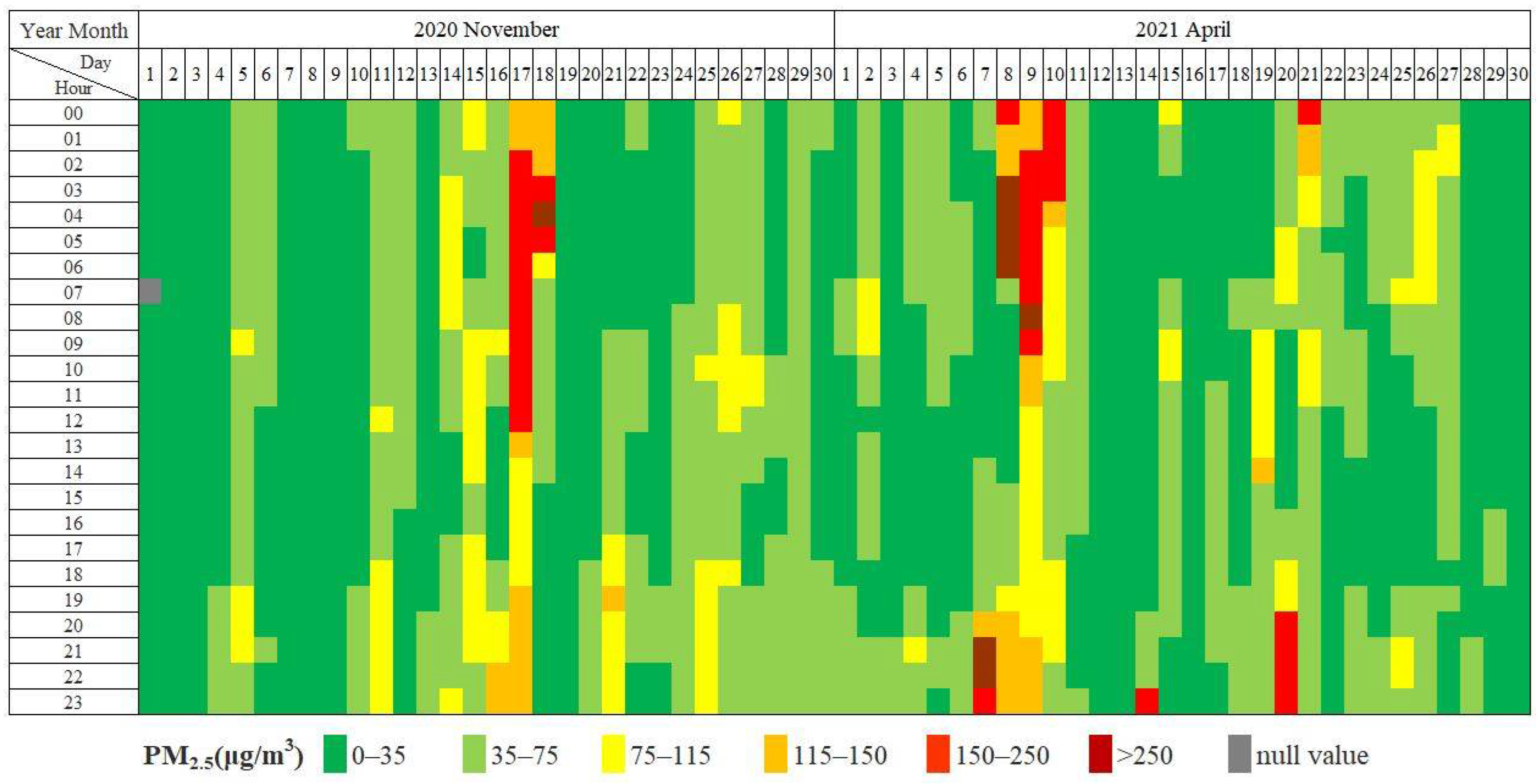
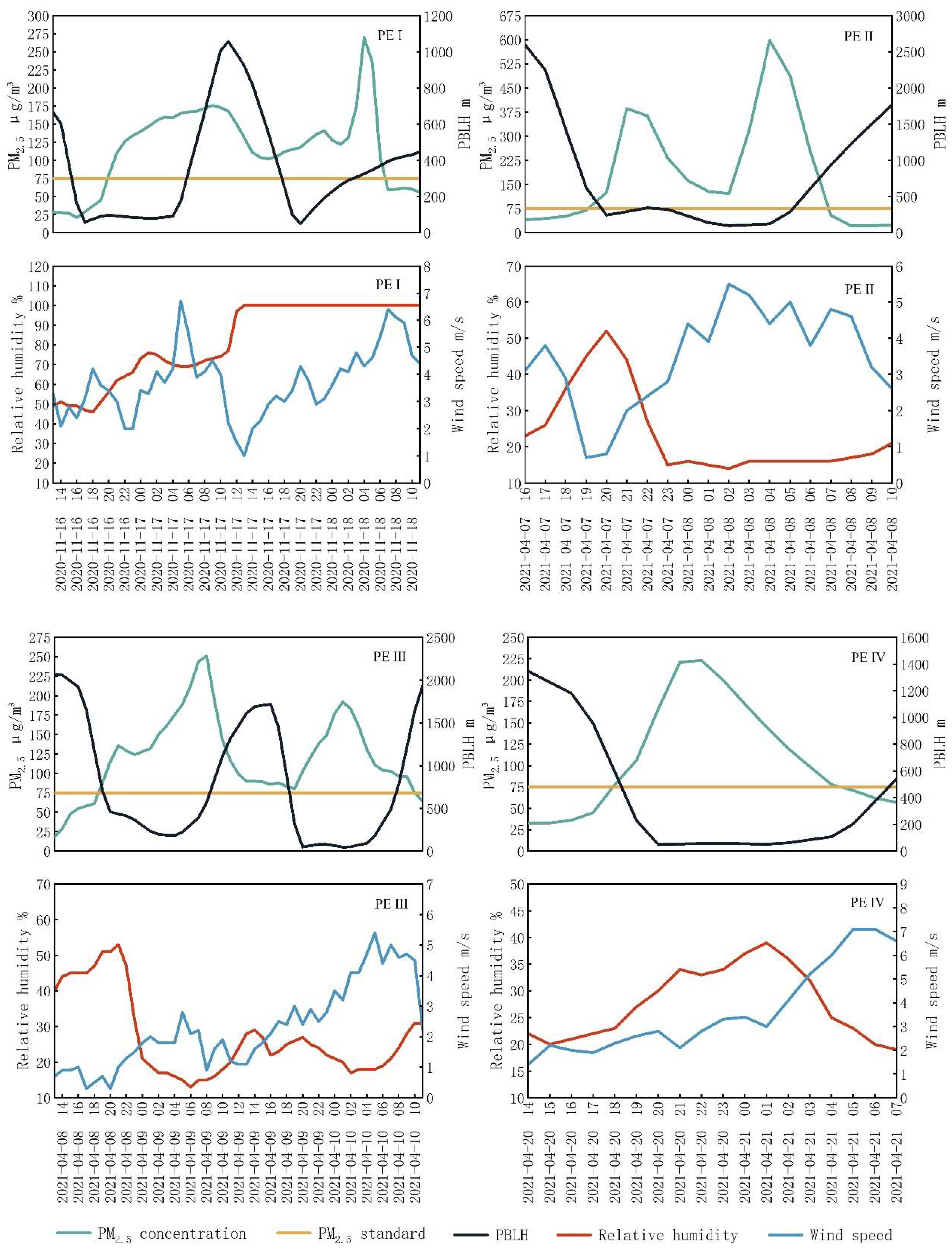
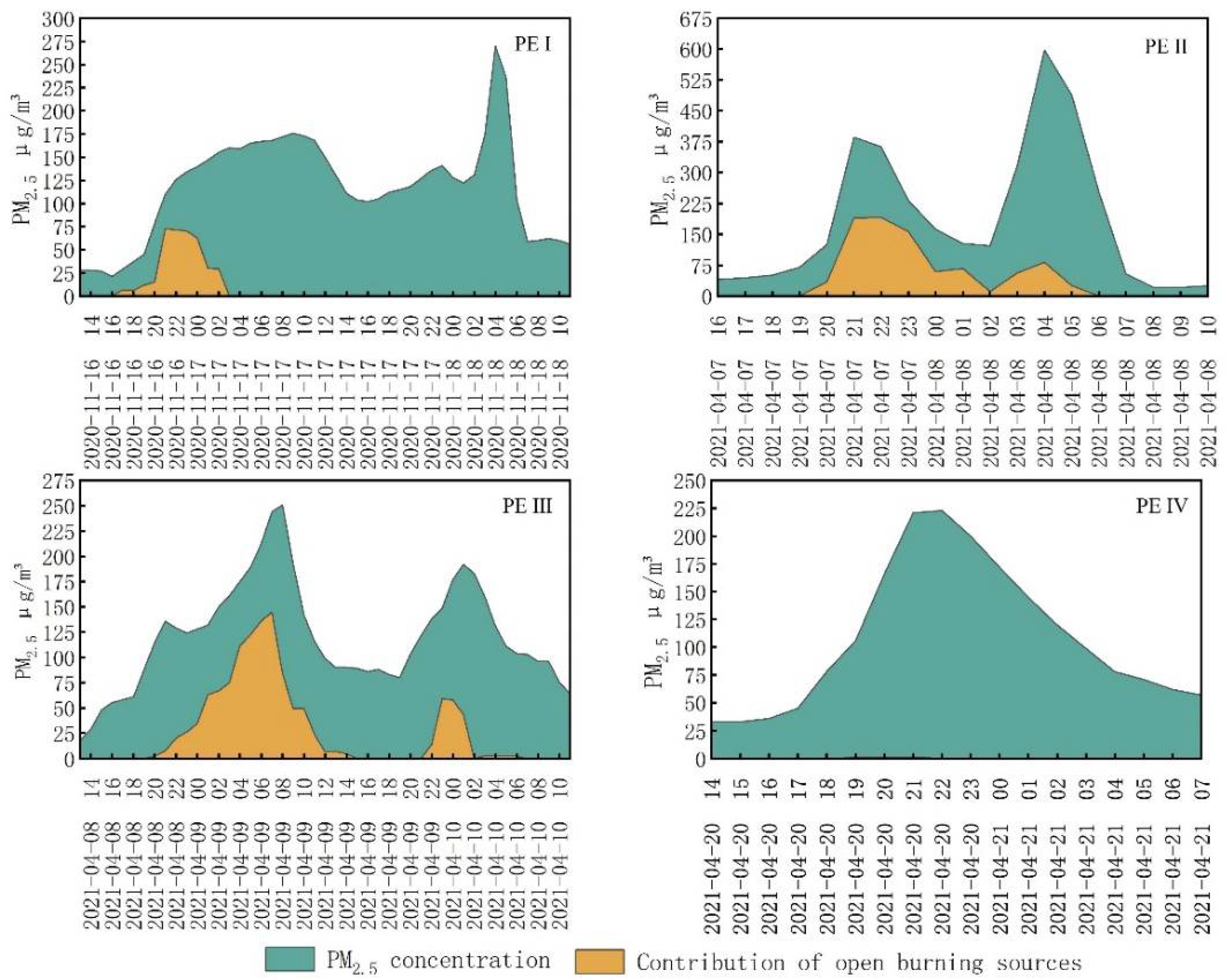
4.1. Characteristics of PM_2.5 Pollution Episodes

According to hourly variations in the PM_2.5 concentrations of Changchun in November 2020 and April 2021 (Figure 5), there were 4 instances of PM_2.5 PEs during the SOB season of 2020–2021, as shown in

Table 1. PM_2.5 pollution episodes in Changchun during the SOB season of 2020–2021.

PE	Start	End	Duration Time	PM2.5 Peak Value	Highest Pollution Level
PE I	20:00 on November 16	7:00 on November 18	35 h	270 μg m−3	Seriously polluted
PE II	20:00 on 7 April	7:00 on 8 April	11 h	598 μg m−3	Seriously polluted
PE III	19:00 on 8 April	11:00 on 10 April	40 h	251 μg m−3	Seriously polluted
PE IV	18:00 on 20 April	4:00 on 21 April	11 h	223 μg m−3	Heavily polluted

.

The fluctuation in hourly PM_2.5 concentration during PEs was significant, as shown in Figure 6. PE I and PE III were characterized by three increase processes, and the duration time of these two PEs was longer, at 35 and 40 h, respectively. For PE II and PE IV, the duration time was shorter (both 11 h); PE II had a bimodal distribution, whereas PE IV had only one peak value. In addition, the peaks of PE I, PE II, and PE III were seriously polluted levels, among which PE II had the highest peak value of 598 μg m⁻³, and the highest pollution level during PE IV is classified as heavily polluted. From the meteorological conditions during the PEs, the peaks of PM_2.5 concentration generally occurred when the urban PBLH level was low. However, not all the peak values of the PEs occurred under static or low wind speed conditions; sometimes, the high PM_2.5 level occurred when urban wind speeds were high. The difference in relative humidity during PEs is obvious, with higher humidity levels and even precipitation during PE I, but lower average relative humidity levels for PE II, PE III, and PE IV.

4.2. Hourly Transport Pathways and Straw Open Burning Sources

Based on hourly backward trajectories with arrival times at hourly intervals, the HTPs and HWFGs during each PE were reconstructed. The spatial distribution of the SOB sources and their inflow time into the city, identified using HTPs and HWFGs, are presented in Figure 7 and Figure 8. From the spatial distribution of the identified SOB sources and their HTPs, we can judge the inflow direction of SOB-caused PM_2.5. In addition, based on the urban ground-monitoring data of hourly PM_2.5 concentration, wind speed, and wind direction, bivariate polar plots of PM_2.5 were plotted to indicate the direction of potential sources [48,49], as shown in Figure 9.

The identified SOB sources of PE I were distributed on the HTPs of only the first sharp increase period of PM_2.5, and the burning area of SOB fire spots was 1.57 ha. This indicated that the air mass carrying SOB-caused PM_2.5 flowed into the city successively during the first sharp increase in PM_2.5, and the inflow direction was between south and southwest. From the bivariate polar plot of PM_2.5 during 16–18 November 2020, based on urban ground-monitoring data, high PM_2.5 concentrations could also be observed at a wind speed of 4–7 m/s when the wind direction was between the south and the southwest.

During PE II, the identified SOB sources were found on the HTPs of the bimodal PM_2.5 increase period, and the burning activity was significant, with hotspot areas up to 20.42 ha. The inflow of the air mass carrying SOB-caused PM_2.5 was mainly between northwest and northeast. According to the bivariate polar plot of PM_2.5 during 7–8 April 2021, a high PM_2.5 level could also be identified when the wind speed was 4–6 m/s in the northwest–northeast direction.

On the HTPs of all three PM_2.5 increase periods of PE III, the identified SOB sources were distributed. The burning area of these SOB fire spots on the transport pathways was 9.02 ha. The inflow direction of air mass was between southeast and southwest. From the bivariate polar plot of PM_2.5 during 9–10 April 2021, high PM_2.5 concentrations could also be observed from the southeast–south wind direction when the wind speed was 3–5 m/s, and medium PM_2.5 concentrations were recorded from the southwestern wind direction when the wind speed was >5 m/s.

On the HTPs of the PM_2.5 increase period of PE IV, the burning area of the identified SOB sources was 2.84 ha. The inflow of the air mass carrying SOB-caused PM_2.5 was mainly from the southeast to the south. According to the bivariate polar plot of PM_2.5 during 20–21 April 2021, a high PM_2.5 level was recorded at a wind speed of 3–4 m/s when the wind direction was from the southeast and south.

The above results demonstrate that the inflow time and direction of the SOB sources identified using HTPs and HWFGs are consistent with (within the range of) the occurrence time and wind direction of the high PM_2.5 level recorded using urban ground-monitoring data; this indicates the reliability of HTP and HWFG reconstruction using backward trajectories. Moreover, no SOB sources were found on the HTPs of some PM_2.5 sharp increase periods, such as the second and third increase during PE I; these high PM_2.5 levels were probably due to local emission activities. Furthermore, due to the long-range transport of regional sources and the complexity of wind-field variation, the orientation of SOB fire spots in rural areas relative to urban areas is not necessarily the inflow direction of the air mass carrying SOB-caused PM_2.5. For example, the majority of SOB fire spots are distributed in the northeast urban area during PE III-1, but the inflow direction of SOB-caused PM_2.5 is from the southeast after passing through the northeastern region. Therefore, using the urban wind direction at a high PM_2.5 concentration to infer SOB source orientation during specific PE may lead to bias, while identifying SOB sources by reconstructing HTPs and HWFGs will eliminate this bias and accurately identify the spatial distribution and orientation of the SOB sources.

4.3. Contributions of Straw Open Burning Sources

The contributions to urban PM_2.5 from SOB sources can be calculated using the TSSTMB model. According to the results shown in Figure 10, we discovered that during the three severe PEs, the contribution of the horizontal transport of SOB sources to the urban PM_2.5 level was more obvious than the contribution during the heavy PE.

In the first PM_2.5 increase period of PE I, the sharp elevation of urban PM_2.5 concentration was closely related to the rapid increase in the share of SOB sources. Especially from 19:00 to 21:00 on 16 November 2020, the percentage of PM_2.5 contribution from SOB was significantly larger, reaching up to 47% with an hourly average contribution of 44 μg m⁻³, and the urban PM_2.5 concentration increased by 144% simultaneously. Unexpectedly, the latter two occurred under the meteorological conditions of precipitation in the city, as shown in Figure 6. Moreover, no SOB fire spots were identified on the corresponding HTPs. This implies that the increasing urban PM_2.5 concentration in the middle-to-late stages was possibly related to local sources. Overall, the total contribution of SOB as regional sources to PE I was 352 μg m⁻³, which accounted for 7% of the accumulated urban PM_2.5 concentration.

The temporal variation in contribution from SOB has a similar trend to the fluctuating urban PM_2.5 concentration during PE II and PE III. The total contributions of SOB sources during PE II and PE III were 872 and 1224 μg m⁻³, respectively, which were 27% and 23% of the corresponding urban accumulated pollution levels. The contribution during the early-increase processes was more significant than the late one. The hourly and stage-average contributions from the SOB sources to urban PM_2.5 pollution levels during PE II and PE III are presented in Table S2. During the first and second increases in PE II, the hourly average contribution from SOB was 116 and 35 μg m⁻³, accounting for 50% and 9.8% of the corresponding urban PM_2.5 level. The proportions of SOB contribution were 38% and 8.0% during the first two and third increases in PE III, and the average contributions were 59 and 9.4 μg m⁻³, respectively. This seemed to indicate that primary pollutants from SOB sources played a more important role in the early stage in the evolution of haze episodes characterized by bimodal or multimodal distribution, and the later peak was not only related to the primary pollutants but also ascribed to the formation of secondary aerosols. This is consistent with the results reported by Sun et al. (2020) [50].

It is interesting that the contribution from SOB during PE IV was low, despite the burning area of the identified SOB fire spots being nearly twice that of PE I. The total contribution from SOB sources during PE IV was 4.9 μg m⁻³, which accounted for 0.31% of the urban cumulative PM_2.5 concentration. This is because of the higher PBLH on the transport pathways of SOB sources and the long transport distance so that the particulate matter produced by straw burning was fully diffused and diluted before flowing to urban areas.

Our results are consistent with other studies and also indicate that straw open burning is the major source of PM, especially during the heavy pollution periods in autumn and spring over Northeast China [51]; a significant portion of the polluted days during the post-harvest season was related to straw burning [52].

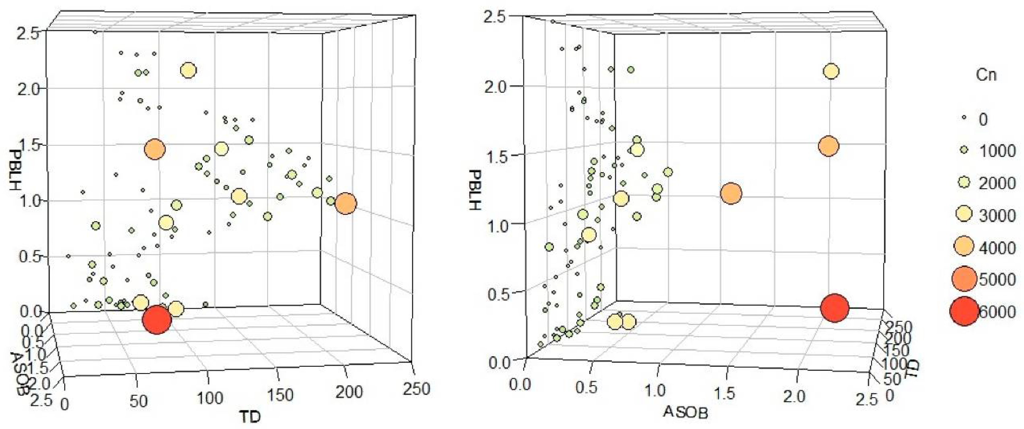
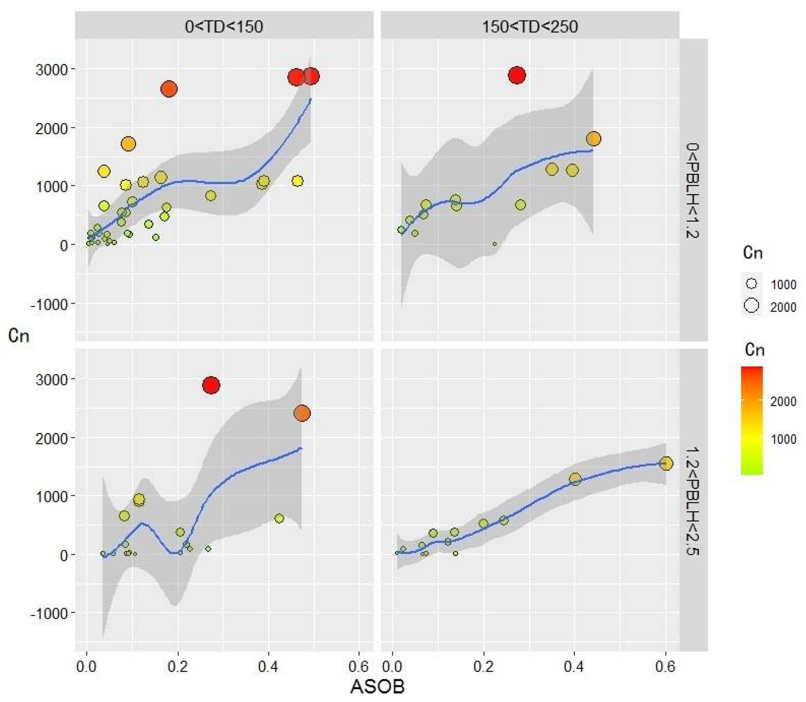
4.4. Analysis of the Impact of Individual Factors

The results demonstrated that the variations in contributions to urban PM_2.5 from SOB sources were significant. According to the TSSTMB model parameters and estimation results, the contributions of SOB sources were mainly determined by the following factors. First, from the perspective of SOB sources and their transport pathways (that is, the first stage of the TSSTMB model), the main influencing factors are the burning area of SOB, the area of the HWFGs, and the average PBLH along the transport pathways; the combined effect of these factors determines the PM_2.5-inflow concentration. Second, in terms of the receptor city (that is, the second stage of the TSSTMB model), meteorological conditions, such as urban PBLH and urban wind speed, affect the degree of dilution and diffusion of PM_2.5-inflow, which ultimately determines the contributions from SOB sources to the urban PM_2.5 level. In this section, the impacts of these two factors will be discussed, respectively.

4.4.1. Impact of Meteorological Conditions on the Receptor City

From Equations (11)–(13), it is found that the hourly contribution of PM_2.5-inflow is closely related to the PM_2.5-inflow concentration and coefficients α and β. Since both α and β are <1, the hourly contribution of a certain PM_2.5-inflow during the first hour of its residence time is greater than that of each hour thereafter. Taking the urban hourly average PM_2.5 concentration of 44.39 μg m⁻³ during the SOB season of 2020–2021 as the background concentration, we can deduce that when the hourly contribution of a certain PM_2.5-inflow during the first hour is <30 μg m⁻³, the urban hourly PM_2.5 during its residence time will not exceed the standard (under the premise of no other PM_2.5-inflow). Therefore, in the following, we discuss the influencing factors of the hourly contribution of PM_2.5-inflow during the first hour of residence time.

According to Equation (11), since the PM_2.5 dry deposition rate and calculation time are constant values (v_d = 0.0005 m/s, τ₁ =3600 s), the hourly contribution of a certain PM_2.5-inflow during the first hour of its residence time is determined by the PM_2.5-inflow concentration and urban PBLH. Therefore, we investigated the relationship between the hourly contribution of PM_2.5-inflow during the first hour and the urban PBLH levels (H_rc(τ₁)) at different specific PM_2.5-inflow concentrations (C_n). As the results show in Figure 11, when urban PBLH is >600 m, even if the PM_2.5-inflow concentration is at an extremely high level of 10,000 μg m⁻³, its hourly contribution is still less than 30 μg m⁻³. This owes to the strong dilution and diffusion of PM_2.5 in the vertical direction. Moreover, when the PM_2.5-inflow concentration is <1000 μg m⁻³, the hourly contribution of PM_2.5-inflow generally does not exceed 30 μg m⁻³, even if the urban PBLH is at a lower height of <600 m. Nevertheless, according to Equations (14) and (15), if continuous PM_2.5-inflow within a few hours enters the city sequentially, its cumulative contributions are likely to induce the urban hourly PM_2.5 to exceed the standard. According to the calculation of residence time, as in Equation (10), for the average diameter of the urban geographic space of Changchun, the residence time of a specific PM_2.5-inflow will not exceed 4 h when the average wind speed is >2 m/s.

Based on the above analysis, we can see that urban PBLH mainly affects the hourly contribution of a specific PM_2.5-inflow, and the average urban wind speed further determines its total contribution by affecting the residence time of PM_2.5-inflow. In addition, it can be deduced that under the conditions of the average urban wind speed being >2 m/s and the interval time of each straw burning event being >4 h, when the urban PBLH is >600 m or the PM_2.5-inflow concentration is <1000 μg m⁻³, the SOB sources will not lead the urban hourly PM_2.5 concentration to exceed the standard. Previous studies have also shown that PM_2.5 concentrations during a haze period in the city of Northeast China were mostly influenced by biomass burning emissions and the atmospheric diffusion conditions of the variation in PBLH and wind speed [53].

4.4.2. Impact of Burning Area, Transport Distance, and Meteorological Conditions along the Transport Pathways

It can be seen from Equation (6) that the PM_2.5-inflow concentration is determined by the conditions of each HWFG on the transport pathway, including multiple factors, such as the SOB burning area in the HWFG, the HWFG area, the PBLH of the HWFGs, and others, and the quantitative relationship between them is iterative and nonlinear. To analyze the impact of the main factors on PM_2.5-inflow concentration, taking each HWFG during each PE as a unit, we calculated the burning area of the SOB sources, their transport distance, the average PBLH along the transport pathway, and their resulting corresponding PM_2.5-inflow concentrations. These main influence factors are shown in a 4D scatterplot in Figure 12. It should be noted that the area of HWFGs in the model parameters is replaced by the indicator of transport distance in the following analysis because transport distance is easier to measure and carry out in the formulation and implementation of SOB management policies.

Note: ASOB, TD, and PBLH in the figure represent the area of the SOB (ha), the transport distance (km), and the PBLH along the transport pathway (km). C_n is the corresponding PM_2.5-inflow concentration (μg m⁻³).

From different viewing angles of the 4D scatter plot, shown in Figure 12, we find that the burning area in each HWFG was within the two ranges of 0.005–0.6 ha and 1–2.5 ha during the 4 PEs, the transport distance was <250 km, and the average PBLH along the transport pathways was <2.5 km. When the burning area was at a high level of 1–2.5 ha, the PM_2.5-inflow concentration reached 3000–6000 μg m⁻³. When the burning area was at a low level of 0.005–0.6 ha, the PM_2.5-inflow concentration was in the range of 2–3000 μg m⁻³, and the variation in the PM_2.5-inflow concentration was significant, with differences in the burning area, transport distance, and average PBLH along the transport pathway.

According to the analysis results in the above section, the PM_2.5-inflow concentration < 1000 μg m⁻³ is one of the “safety limits” to ensure urban hourly PM_2.5 concentrations do not exceed the standard. To determine the conditions for making the PM_2.5-inflow concentration < 1000 μg m⁻³, the relationships between the burning area (at a low level of 0.005–0.6 ha) and the PM_2.5-inflow concentration were fitted under four combinatorial conditions of transport distance and average PBLH along the transport pathway.

It can be seen from the fitting results shown in Figure 13 that under the conditions of shorter transport distance (<150 km) and lower PBLH along the transport pathway (<1.2 km), the burning area limit must be <0.18 ha to make the PM_2.5-inflow concentration <1000 μg m⁻³. Second, under the conditions of shorter transport distance (<150 km) but higher PBLH along the transport pathway (1.2–2.5 km), the burning area limit should be <0.24 ha. Third, when the transport distance is longer than 150–250 km but the PBLH along the transport pathway is at a lower level of <1.2 km, the burning area limit is 0.27 ha. Fourth, when the transport distance is longer than 150–250 km and the PBLH along the transport pathway is at a higher level close to 1.2–2.5 km, the burning area limit is 0.35 ha. Some studies also proved that the conditions at burn sites, especially emission intensity and meteorological factors, as well as transport distance, play significant roles in the regional transport of PM_2.5; moreover, they verified that not only local emission control, but also horizontal atmospheric transport and meteorological conditions can facilitate the cross-regional development of accurate prediction models and effective pollution control measures [54,55].

4.5. Policy Implications

According to the analysis results of the impact of individual factors, some policy suggestions on SOB management and control are put forward as follows. When the average urban wind speed is <2 m/s, it is suggested that SOB should be strictly prohibited on farmland within 250 km of the city’s upwind direction. It is better to proceed with SOB activity under the meteorological conditions of urban wind speed > 2 m/s and urban PBLH > 600 m; moreover, the interval time of each SOB activity should be more than 4 h, and the burning area of each SOB activity should preferably not exceed 2.5 ha. When urban wind speed is >2 m/s but urban PBLH is <600 m, the burning area should be further strictly controlled according to the distance from the burning site to the receptor city and the average PBLH along possible transport pathways: under the conditions of shorter transport distance (<150 km) and lower PBLH along the transport pathway (<1.2 km), the burning area limit should be 0.18 ha; under the conditions of shorter transport distance (<150 km) but higher PBLH along the transport pathway (1.2~2.5 km), the burning area limit should be 0.24 ha; when the transport distance is within 150~250 km but the PBLH along the transport pathway is <1.2 km, the burning area limit should be 0.27 ha; when the transport distance is within 150~250 km and the PBLH along the transport pathway is close to 1.2~2.5 km, the burning area limit should be 0.35 ha.

5. Conclusions

In this study, an integrated method based on ArcGIS geoprocessing was presented to quantify the contribution of external sources of SOB to elevated urban PM_2.5 concentrations during specific haze episodes at a high temporal resolution of 1 h. The results of this study showed that during the SOB season in 2020–2021, Changchun experienced severe urban PEs three times (PE I, PE II, and PE III) and heavy urban PE once (PE IV), which lasted 97 h in total. Additionally, we discovered that the total PM_2.5 contributions from SOB sources were 352 μg m⁻³, 872 μg m⁻³, and 1224 μg m⁻³ during the three instances of severe PEs, respectively, accounting for 7%, 27%, and 23% of the urban cumulative PM_2.5 level; these were more obvious than contribution during the heavy PE. During PE IV, the total PM_2.5 contribution from SOB sources (4.9 μg m⁻³) was only 0.31% of the urban cumulative PM_2.5 level; this is mainly due to the long transport distance of SOB sources and the higher PBLH along the transport pathways. In addition, it seemed that primary pollutants from SOB sources played a more important role in the early stage of the evolution of haze episodes, characterized by bimodal or multimodal distribution, and the later peak was possibly not only related to the primary pollutants of SOB but also ascribed to the formation of secondary aerosols.

The advantages of our integrated method are mainly the following. First, the spatial and temporal distribution scope of potential SOB sources associated with a specific PE could be determined via reconstructed HTPs and HWFGs, and the SOB fire spots associated with elevated PM_2.5 concentrations during PEs could be identified. Moreover, the TSSTMB model linked the spatial scope of external SOB sources, their transport pathways, and the hourly pollution level in the receptor city. Furthermore, the interactive model based on ArcGIS geoprocessing can integrate different types of multi-source datasets. Although secondary particulate matter formation during transport should be further supplemented in future directions, we believe this integrated method is physically realistic regarding the regional transport of SOB-caused primary PM_2.5. Additionally, the refined policy recommendations put forward in this paper are applicable to cities, such as Changchun, which are located in the major grain-producing areas of the plains; this would help to change the implementation of planned and systematic SOB in rural areas to minimize the adverse effects on urban air quality.

References

1. Poulain, L.; Fahlbusch, B.; Spindler, G.; Mueller, K.; van Pinxteren, D.; Wu, Z.; Iinuma, Y.; Birmili, W.; Wiedensohler, A.; Herrmann, H. Source apportionment and impact of long-range transport on carbonaceous aerosol particles in central Germany during HCCT-2010. Atmos. Chem. Phys. 2021, 21, 3667–3684. [Google Scholar] [CrossRef]
2. Ravindra, K.; Singh, T.; Sinha, V.; Sinha, B.; Paul, S.; Attri, S.D.; Mor, S. Appraisal of regional haze event and its relationship with PM2. 5 concentration, crop residue burning and meteorology in Chandigarh, India. Chemosphere 2021, 273, 128562. [Google Scholar] [CrossRef] [PubMed]
3. Wang, Q.L.; Wang, L.L.; Li, X.R.; Xin, J.Y.; Liu, Z.R.; Sun, Y.; Liu, J.D.; Zhang, Y.J.; Du, W.; Jin, X.; et al. Emission characteristics of size distribution, chemical composition and light absorption of particles from field-scale crop residue burning in Northeast China. Sci. Total Environ. 2020, 710, 136304. [Google Scholar] [CrossRef]
4. Yin, S.; Wang, X.F.; Xiao, Y.; Tani, H.; Zhong, G.S.; Sun, Z.Y. Study on spatial distribution of crop residue burning and PM2.5 change in China. Environ. Pollut. 2017, 220, 204–221. [Google Scholar] [CrossRef]
5. Chen, Y.; Xie, S. Characteristics and formation mechanism of a heavy air pollution episode caused by biomass burning in Chengdu, Southwest China. Sci. Total Environ. 2014, 473, 507–517. [Google Scholar] [CrossRef] [PubMed]
6. Cheng, Y.H.; Yang, L.S. Characteristics of ambient black carbon mass and sizeresolved particle number concentrations during corn straw open-field burning episode observations at a rural site in southern Taiwan. Int. J. Environ. Res. Publ. Health 2016, 13, 688. [Google Scholar] [CrossRef]
7. Andreae, M.O. Emission of trace gases and aerosols from biomass burning—An updated assessment. Atmos. Chem. Phys. 2019, 19, 8523–8546. [Google Scholar] [CrossRef]
8. Nguyen, L.S.P.; Huang, H.-Y.; Lei, T.L.; Bui, T.T.; Wang, S.-H.; Chi, K.H.; Sheu, G.-R.; Lee, C.-T.; Ou-Yang, C.-F.; Lin, N.-H. Characterizing a landmark biomass-burning event and its implication for aging processes during long-range transport. Atmos. Environ. 2020, 241, 117766. [Google Scholar] [CrossRef]
9. Salvador, P.; Almeida, S.; Cardoso, J.; Almeida-Silva, M.; Nunesc, T.; Cerqueira, M.; Alves, C.; Reis, M.; Chaves, P.; Artíñano, B.; et al. Composition and origin of pm in Cape Verde: Characterization of long-range transport episodes. Atmos. Environ. 2016, 127, 326–339. [Google Scholar] [CrossRef]
10. Zhou, Y.; Xing, X.; Lang, J.; Chen, D.; Cheng, S.; Wei, L.; Wei, X.; Liu, C. A comprehensive biomass burning emission inventory with high spatial and temporal resolution in China. Atmos. Chem. Phys. 2017, 17, 2839–2864. [Google Scholar] [CrossRef] [Green Version]
11. Hong, C.; Zhang, Q.; Zhang, Y.; Davis, S.; Tong, D.; Zheng, Y.; Liu, Z.; Guan, D.; He, K.; Schellnhuber, H. Impacts of climate change on future air quality and human health in China. Proc. Natl. Acad. Sci. USA 2019, 116, 17193–17220. [Google Scholar] [CrossRef] [PubMed]
12. Annan, K.; Ma, Q.; Lund, M.; Wang, S. Population-weighted exposure to pm pollution in China: An integrated approach. Environ. Int. 2018, 120, 111–120. [Google Scholar] [CrossRef] [PubMed]
13. Hsu, Y.; Holsen, T.M.; Hopke, P.K. Comparison of hybrid receptor models to locate PCB sources in Chicago. Atmos. Environ. 2003, 37, 545–562. [Google Scholar] [CrossRef]
14. Gildemeister, A.E.; Hopke, P.K.; Kim, E. Sources of fine urban particulate matter in Detroit, MI. Chemosphere 2007, 69, 1064–1074. [Google Scholar] [CrossRef] [PubMed]
15. Weiss-Penzias, P.S.; Gustin, M.S.; Lyman, S.N. Sources of gaseous oxidized mercury and mercury dry deposition at two southeastern U.S. sites. Atmos. Environ. 2011, 45, 4569–4579. [Google Scholar] [CrossRef]
16. Seibert, P.; Kromp-Kolb, H.; Baltensperger, U.; Jost, D.T.; Schwikowski, M.; Kasper, A.; Puxbaum, H. Trajectory analysis of aerosol measurements at high alpine sites. In Transport and Transformation of Pollutants in the Troposphere; Borrell, P.M., Borrell, P., Cvitas, T., Seiler, W., Eds.; Academic Publishing: Den Haag, The Netherlands, 1994; pp. 689–693. [Google Scholar]
17. Han, Y.-J.; Holsen, T.M.; Hopke, P.K. Estimation of source locations of total gaseous mercury measured in New York State using trajectory-based models. Atmos. Environ. 2007, 41, 6033–6047. [Google Scholar] [CrossRef]
18. Xie, Y.; Berkowitz, C.M. The use of conditional probability functions and potential source contribution functions to identify source regions and advection pathways of hydrocarbon emissions in Houston, Texas. Atmos. Environ. 2007, 41, 5831–5847. [Google Scholar] [CrossRef]
19. Cheng, I.; Zhang, P.; Blanchard, P.; Dalziel, J.; Tordon, R. Concentration weighted trajectory approach to identifying potential sources of speciated atmospheric mercury at an urban coastal site in Nova Scotia, Canada. Atmos. Chem. Phys. 2013, 13, 6031–6048. [Google Scholar] [CrossRef]
20. Wang, L.; Wei, Z.; Wei, W.; Fu, J.S.; Meng, C.; Ma, S. Source apportionment of PM2.5 in top polluted cities in Hebei, China using the CMAQ model. Atmos. Environ. 2015, 122, 723–736. [Google Scholar] [CrossRef]
21. Itahashi, S.; Uno, I.; Kim, S. Source Contributions of Sulfate Aerosol over East Asia Estimated by CMAQ-DDM. Environ. Sci. Technol. 2012, 46, 6733–6741. [Google Scholar] [CrossRef]
22. Zhao, B.; Wang, S.X.; Xing, J.; Fu, K.; Fu, J.S.; Jang, C.; Zhu, Y.; Dong, X.Y.; Gao, Y.; Wu, W.J.; et al. Assessing the nonlinear response of fine particles to precursor emissions: Development and application of an extended response surface modeling technique v1.0. Geosci. Model Dev. 2015, 8, 115–128. [Google Scholar] [CrossRef]
23. Yu, Y.; Xu, H.; Jiang, Y.; Chen, F.; Cui, X.; He, J.; Liu, D. A modeling study of PM2.5 transboundary during a winter severe haze dpisode in Southern Yangtze River Delta, China. Atmos. Res. 2021, 248, 105159. [Google Scholar] [CrossRef]
24. Chang, X.; Wang, S.; Zhao, B.; Cai, S.; Hao, J. Assessment of inter-city transport of particulate matter in the Beijing–Tianjin–Hebei region. Atmos. Chem. Phys. 2018, 18, 4843–4858. [Google Scholar] [CrossRef]
25. Zhang, H.; Cheng, S.; Yao, S.; Wang, X.; Zhang, J. Multiple perspectives for modeling regional PM2.5 transport across cities in the Beijing-Tianjin-Hebei region during haze episodes. Atmos. Environ. 2019, 212, 22–35. [Google Scholar] [CrossRef]
26. Wu, Y.J.; Wang, P.; Yu, S.C.; Wang, L.Q.; Li, P.F.; Li, Z.; Mehmood, K.; Liu, W.P.; Wu, J.; Lichtfouse, E.; et al. Residential emissions predicted as a major source of fne particulate matter in winter over the Yangtze River Delta, China. Environ. Chem. Lett. 2018, 16, 1117–1127. [Google Scholar] [CrossRef]
27. Wu, J.R.; Li, G.H.; Cao, J.J.; Bei, N.F.; Wang, Y.C.; Feng, T.; Huang, R.H.; Liu, S.X.; Zhang, Q.; Tie, X.X. Contributions of trans-boundary transport to summertime air quality in Beijing, China. Atmos. Chem. Phys. 2017, 17, 2035–2051. [Google Scholar] [CrossRef]
28. Fu, X.; Cheng, Z.; Wang, S.X.; Hua, Y.; Xing, J.; Hao, J.M. Local and regional contributions to fne particle pollution in winter of the Yangtze River Delta, China. Aerosol Air Qual. Res. 2016, 16, 1067–1080. [Google Scholar] [CrossRef]
29. Kwok, R.H.F.; Baker, K.R.; Napelenok, S.L.; Tonnesen, G.S. Photochemical grid model implementation and application of VOC, NOx, and O3 source apportionment. Geosci. Model Dev. 2015, 8, 99–114. [Google Scholar] [CrossRef]
30. In, H.-J.; Byun, D.W.; Park, R.; Moon, N.-K.; Kim, S.; Zhong, S. Impact of transboundary transport of carbonaceous aerosols on the regional air quality in the United States: A case study of the South American wildland fire of May 1998. J. Geophys. Res. Atmos. 2007, 112, D07201. [Google Scholar] [CrossRef]
31. An, J.; Li, J.; Zhang, W.; Chen, Y.; Qu, Y.; Xiang, W. Simulation of transboundary transport fluxes of air pollutants among Beijing, Tianjin, and Hebei Province of China. Acta Sci. Circumstantiae 2012, 32, 2684–2692. [Google Scholar]
32. Jenner, S.L.; Abiodun, B.J. The transport of atmospheric sulfur over Cape Town. Atmos. Environ. 2013, 79, 248–260. [Google Scholar] [CrossRef]
33. Yokelson, R.J.; Burling, I.R.; Urbanski, S.P.; Atlas, E.L.; Adachi, K.; Buseck, P.R.; Wiedinmyer, C.; Akagi, S.K.; Toohey, D.W.; Wold, C.E. Trace gas and particle emissions from open biomass burning in Mexico. Atmos. Chem. Phys. 2011, 11, 6787–6808. [Google Scholar] [CrossRef]
34. Bureau of Statistics of Jilin Province. Jilin Statistical Yearbook; Jilin University Press: Changchun, China, 2021.
35. Chen, W.W.; Tong, D.Q.; Dan, M.; Zhang, S.C.; Zhang, X.L.; Pan, Y.P. Typical atmospheric haze during crop harvest season in northeastern China: A case in the Changchun region. J. Environ. Sci. 2017, 54, 101–113. [Google Scholar] [CrossRef] [PubMed]
36. Zhao, H.; Yang, G.; Tong, D.Q.; Zhang, X.; Xiu, A.; Zhang, S. Interannual and seasonal variability of greenhouse gases and aerosol emissions from biomass burning in Northeastern China constrained by satellite observations. Remote Sens. 2021, 13, 1005. [Google Scholar] [CrossRef]
37. Global Data Assimilation System (GDAS1) Archive Information. Available online: ftp://ftp.arl.noaa.gov/pub/archives/gdas1 (accessed on 16 February 2022).
38. Hybrid Single Particle Lagrangian Integrated Trajectory (HYSPLIT-4) Model. Available online: http://www.arl.noaa.gov/ready/open/hysplit4.html (accessed on 16 February 2022).
39. Wang, Y.Q.; Zhang, X.Y.; Draxler, R. TrajStat: GIS-based software that uses various trajectory statistical analysis methods to identify potential sources from long-term air pollution measurement data. Environ. Model. Softw. 2009, 24, 938–939. [Google Scholar] [CrossRef]
40. TrajStat Software. Available online: http://www.meteothink.org/docs/trajstat/index.html (accessed on 16 February 2022).
41. Cao, F.; Zhang, S.-C.; Kawamura, K.; Zhang, Y.-L. Inorganic markers, carbonaceous components and stable carbon isotope from biomass burning aerosols in Northeast China. Sci. Total Environ. 2016, 572, 1244–1251. [Google Scholar] [CrossRef]
42. Pan, X.L.; Kanaya, Y.; Wang, Z.F.; Komazaki, Y.; Taketani, F.; Akimoto, H.; Pochanart, P. Variations of carbonaceous aerosols from open crop residue burning with transport and its implication to estimate their lifetimes. Atmos. Environ. 2013, 74, 301–310. [Google Scholar] [CrossRef]
43. Himawari-8 Advanced Himawari Imager (AHI) Fire Product. Available online: ftp://ftp.ptree.jaxa.jp (accessed on 16 February 2022).
44. MODIS Land Cover Product (MCD12Q1). Available online: https://lpdaac.usgs.gov/products/mcd12q1v006/ (accessed on 16 February 2022).
45. Zhang, X.; Kondragunta, S.; Ram, J.; Schmidt, C.; Huang, H.C. Near-real-time global biomass burning emissions product from geostationary satellite constellation. J. Geophys. Res. Atmos. 2012, 117, D14201. [Google Scholar] [CrossRef]
46. Yang, G.; Zhao, H.; Tong, D.Q.; Xiu, A.; Zhang, X.; Gao, C. Impacts of post-harvest open biomass burning and burning ban policy on severe haze in the Northeastern China. Sci. Total Environ. 2020, 716, 136517. [Google Scholar] [CrossRef]
47. Jorquera, H. Air quality at Santiago, Chile: A box modeling approach II. PM2.5, coarse and PM10 particulate matter fractions. Atmos. Environ. 2002, 36, 331–344. [Google Scholar] [CrossRef]
48. Carslaw, D.C.; Ropkins, K. Openair—an R package for air quality data analysis. Environ. Model. Softw. 2012, 27, 52–61. [Google Scholar] [CrossRef]
49. Grange, S.K.; Lewis, A.C.; Carslaw, D.C. Source apportionment advances using polar plots of bivariate correlation and regression statistics. Atmos. Environ. 2016, 145, 128–134. [Google Scholar] [CrossRef]
50. Sun, X.Z.; Wang, K.; Li, B.; Zong, Z.; Shi, X.F.; Ma, L.X.; Fu, D.L.; Thapa, S.; Qi, H.; Tian, C.G. Exploring the cause of PM2.5 pollution episodes in a cold metropolis in China. J. Clean. Prod. 2020, 256, 120275. [Google Scholar] [CrossRef]
51. Chen, W.; Li, J.; Bao, Q.; Gao, Z.; Cheng, T.; Yu, Y. Evaluation of straw open burning prohibition effect on provincial air quality during October and November 2018 in Jilin Province. Atmosphere 2019, 10, 375. [Google Scholar] [CrossRef]
52. Li, Y.; Liu, J.; Han, H.; Zhao, T.; Zhang, X.; Zhuang, B.; Wang, T.; Chen, H.; Wu, Y.; Li, M. Collective impacts of biomass burning and synoptic weather on surface PM2.5 and CO in Northeast China. Atmos. Environ. 2019, 213, 64–80. [Google Scholar] [CrossRef]
53. Li, W.G.; Duan, F.K.; Zhao, Q.; Song, W.W.; Cheng, Y.; Wang, X.Y.; Li, L.; He, K.B. Investigating the effect of sources and meteorological conditions on wintertime haze formation in Northeast China: A case study in Harbin. Sci. Total Environ. 2021, 801, 149631. [Google Scholar] [CrossRef]
54. Meng, C.; Cheng, T.; Gu, X.; Shi, S.; Wang, W.; Wu, Y.; Bao, F. Contribution of meteorological factors to particulate pollution during winters in Beijing. Sci. Total Environ. 2019, 656, 977–985. [Google Scholar] [CrossRef]
55. Li, X.; Cheng, T.; Shi, S.; Guo, H.; Wu, Y.; Lei, M.; Zuo, X.; Wang, W.; Han, Z. Evaluating the impacts of burning biomass on PM2.5 regional transport under various emission conditions. Sci. Total Environ. 2021, 793, 148481. [Google Scholar] [CrossRef]
Figure 1. Topography (a) and farmland distribution (b) in Jilin Province. The inset is the urban area of Changchun and its atmospheric environmental and meteorological ground-monitoring sites.
Remotesensing 14 04671 g001
Figure 2. Framework and procedures of the GIS-based integrated method in this study.
Remotesensing 14 04671 g002
Figure 3. Schematic of reconstructing hourly transport pathways and wind-field grids. Note: (a): Hourly backward trajectories with hourly arrival times of April 2021; (b): Hourly backward trajectories with hourly arrival times from 17:00 on 7 April to 7:00 on 8 April; (c): Hourly backward trajectories with hourly arrival times from 17:00 to 23:00 on 7 April; (d): Pathway lines indicating the geographic position of a moving air mass at the same moment as the pathway time; (e): Spatiotemporal distribution of the wind-field grids, for example, the air mass arriving at receptor city at 21:00–22:00 on 7 April 2021 was distributed in the region of the blue grid at 6:00–7:00 on 7 April 2021.
Remotesensing 14 04671 g003
Figure 4. Schematic diagram of two-stage spatiotemporal multi-box modeling based on hourly wind-field grids.
Remotesensing 14 04671 g004
Figure 5. Calendar plot of hourly PM2.5 concentrations of Changchun during the SOB season of 2020–2021.
Remotesensing 14 04671 g005
Figure 6. Hourly variations in PM2.5 concentrations, PBLH, wind speed, and relative humidity for Changchun during each PE (time format: yyyy-mm-dd hh).
Remotesensing 14 04671 g006
Figure 7. The inflow time into the city of the PM2.5 from identified straw open burning sources.
Remotesensing 14 04671 g007
Figure 8. Spatial distribution of hourly transport pathways and hourly wind-field grids during each PE and the identified straw open burning fire spots. Note: to avoid spatial overlap, HWFGs of PE II are divided and shown in two panels of PE II1 and PE II2, whose arrival times are from 17:00 to 23:00 on 7 April, and from 23:00 on 7 April to 8:00 on 8 April, respectively. Analogously, HWFGs of PE III are divided and shown in two panels of PE III 1 and PE III 2, whose arrival times are from 13:00 on 8 April to 7:00 on 9 April, and from 7:00 on 9 April to 11:00 on 10 April, respectively.
Remotesensing 14 04671 g008
Figure 9. Bivariate polar plots of PM2.5 during, and for several hours before and after, PEs, based on urban ground-monitoring data of hourly PM2.5 concentration, wind speed, and wind direction.
Remotesensing 14 04671 g009
Figure 10. The contribution from straw open burning sources to urban PM2.5 levels.
Remotesensing 14 04671 g010
Figure 11. Relationship between the hourly contribution of PM2.5-inflow and urban PBLH at different specific PM2.5-inflow concentrations.
Remotesensing 14 04671 g011
Figure 12. Distribution of burning area, transport distance, average PBLH along the transport pathway, and the corresponding PM2.5-inflow concentration in the HWFGs during each PE.
Remotesensing 14 04671 g012
Figure 13. Relationships between burning area and PM2.5-inflow concentration fitted under four combinatorial conditions of transport distance and average PBLH along the transport pathway. Note: ASOB, TD, and PBLH in the figure represent area of SOB (ha), transport distance (km), and PBLH along the transport pathway (km). Cn is the corresponding PM2.5-inflow concentration (μg m−3).
Remotesensing 14 04671 g013