
Multi-Source Remote Sensing Pretraining Based on Contrastive Self-Supervised Learning


Abstract
:1. Introduction
- (1)
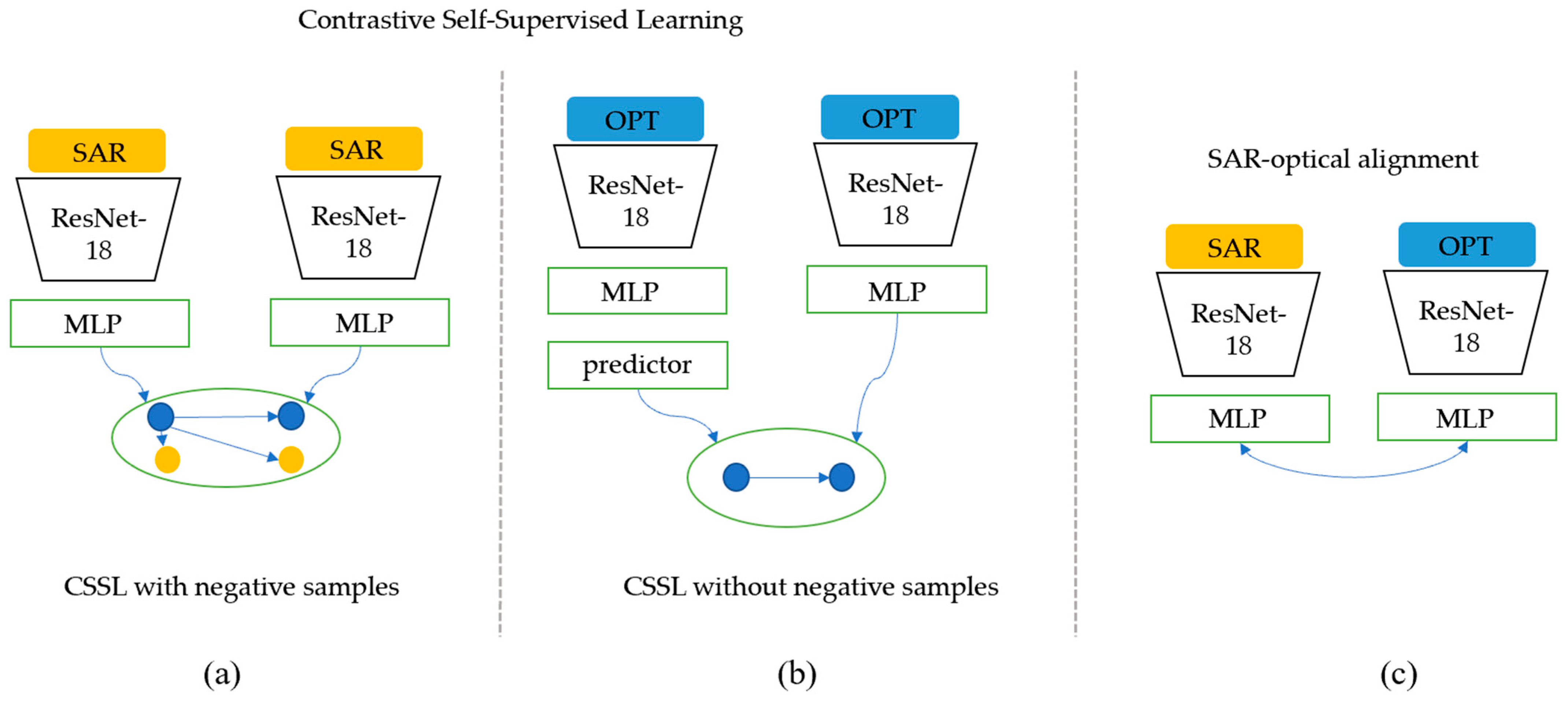
- We introduce the CSSL method with negative samples and the CSSL method without negative samples into multi-source remote-sensing image applications simultaneously, and we systematically compare the effectiveness of the two different frameworks for remote-sensing image classification for the first time.
- (2)
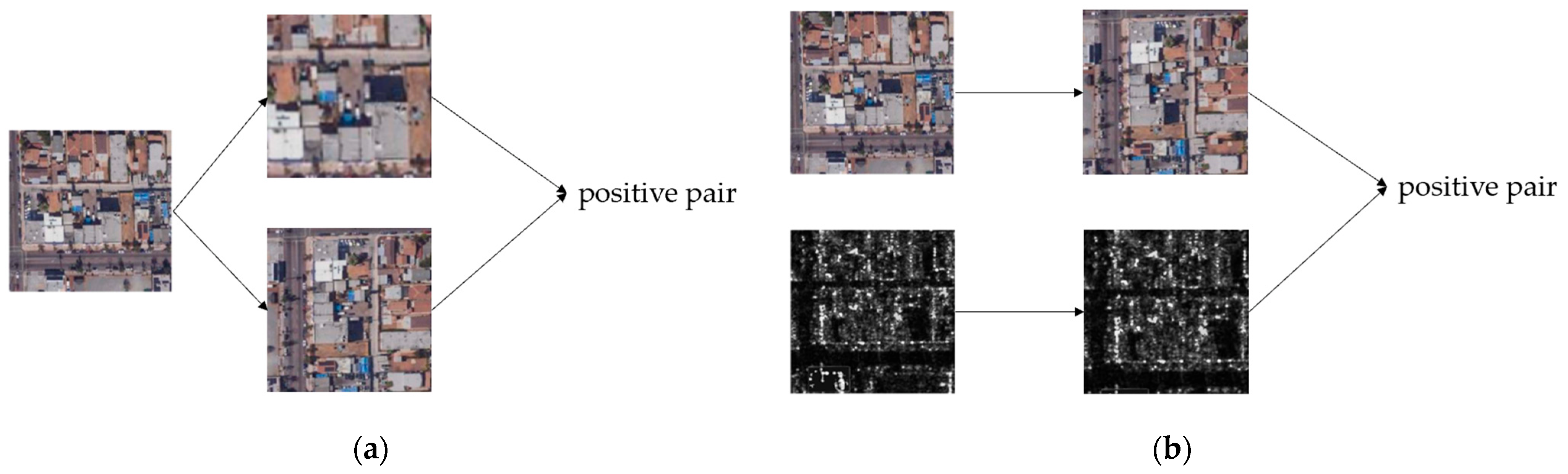
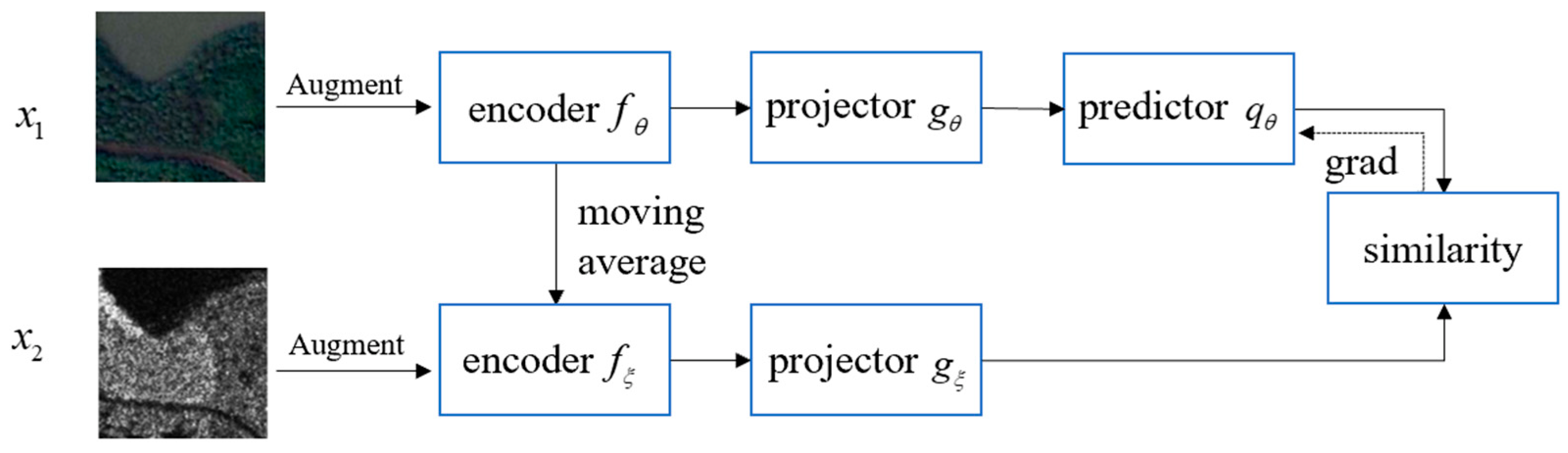
- We determine through analysis that the registered SAR-optical images have structural consistency and can be used as natural contrastive samples that can drive the Siamese network without negative samples to learn shared features of SAR-optical images.
- (3)
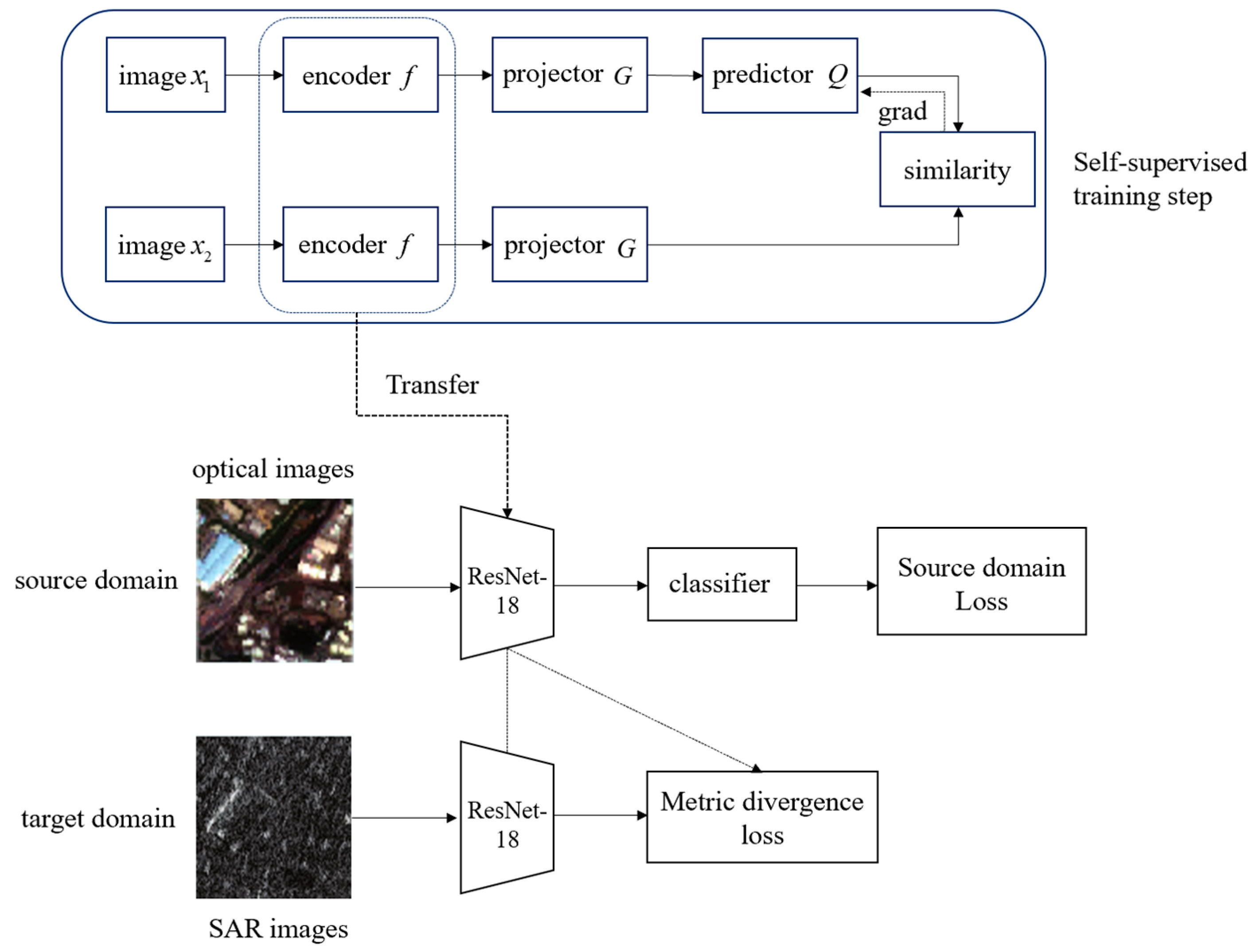
- We explore the application of self-supervised pretrained networks to the downstream domain adaptation task of optical transfer to SAR for the first time.
2. Methods
2.1. Multi-Source Contrastive Self-Supervised Method with Negative Samples
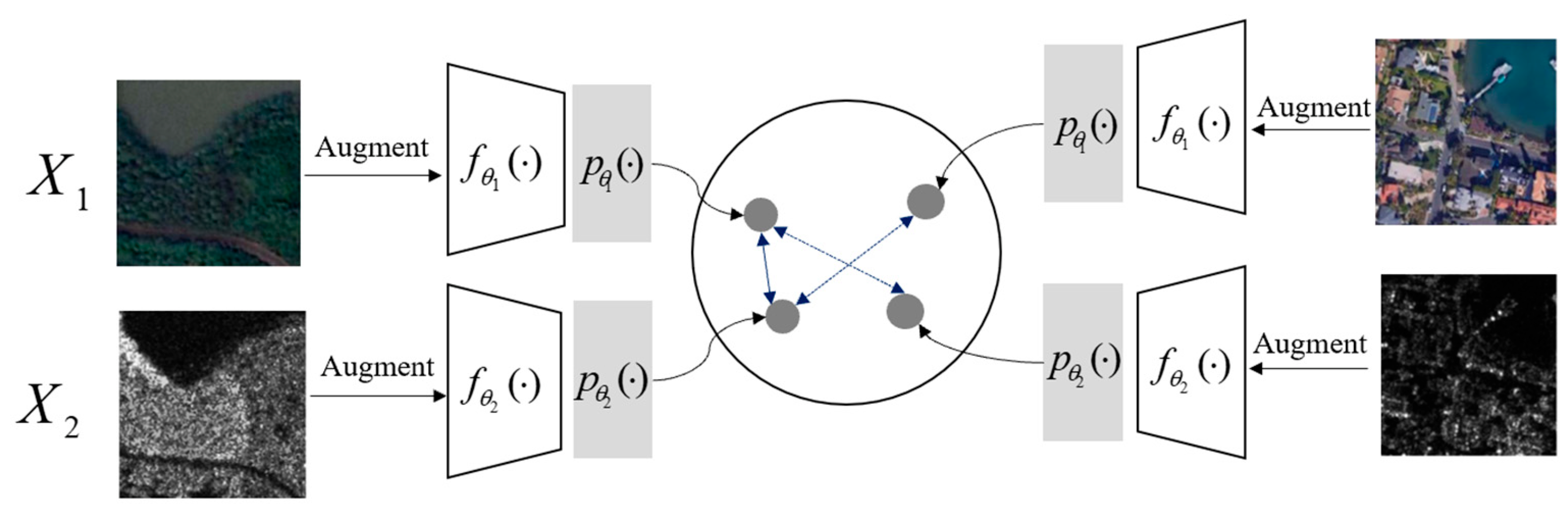
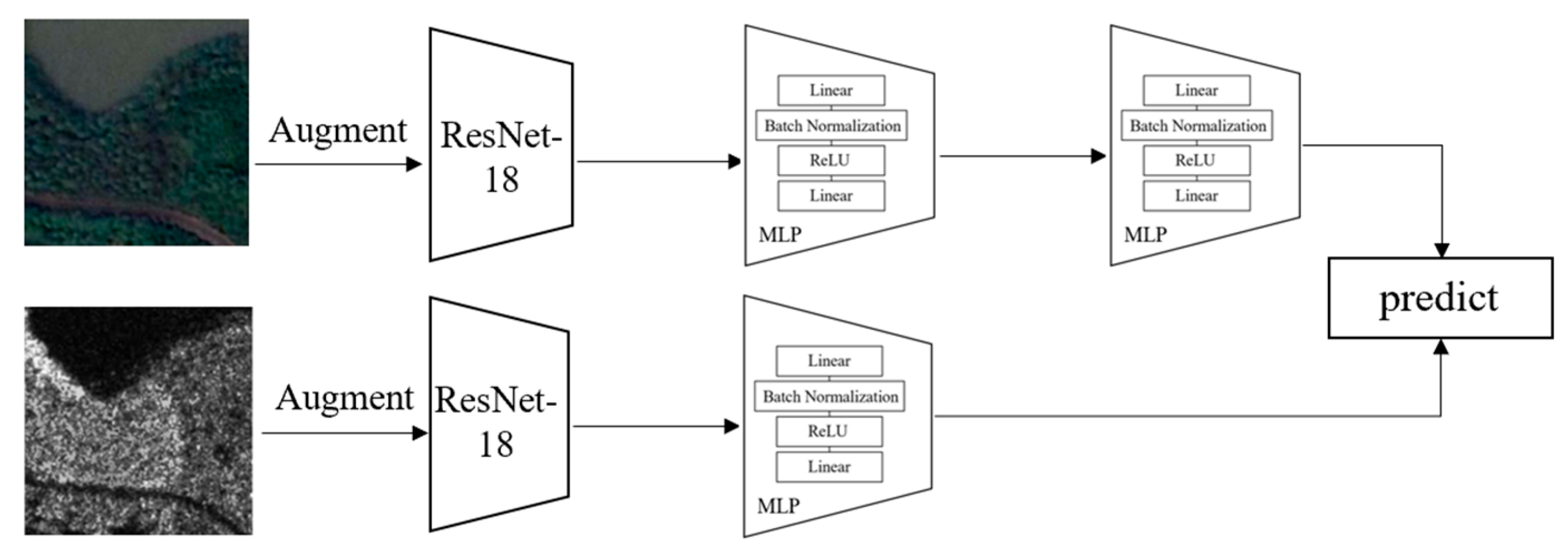
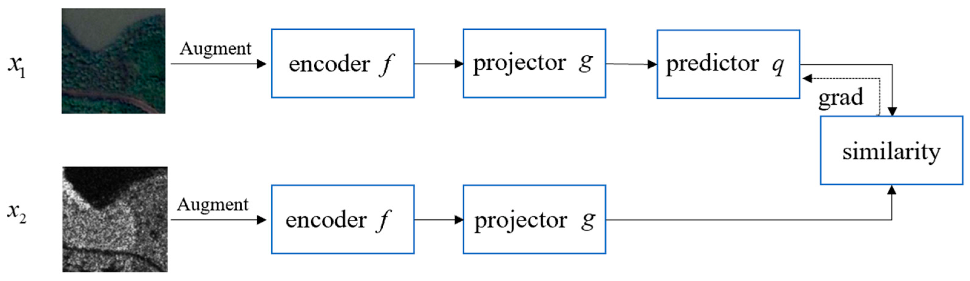
2.2. Multi-Source Contrastive Self-Supervised Method without Negative Samples
2.3. Domain Adaption Based on Multi-Source Contrastive Self-Supervised Pretraining
3. Experiments
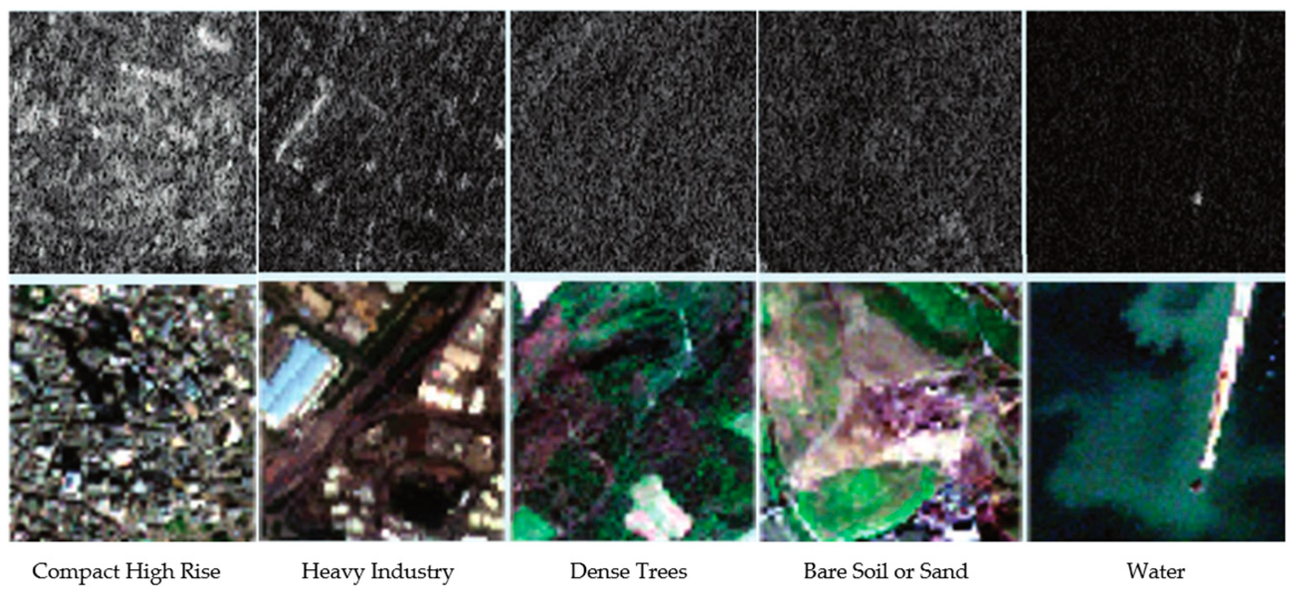
3.1. Datasets
3.2. Experimental Setup
3.2.1. Self-Supervised Network Training
3.2.2. Downstream Classification Task
3.2.3. Downstream Domain Adaption Task
4. Results
4.1. Comparison on the Linear Classification Task
4.2. Comparison on Finetuning Results
4.3. Visualization
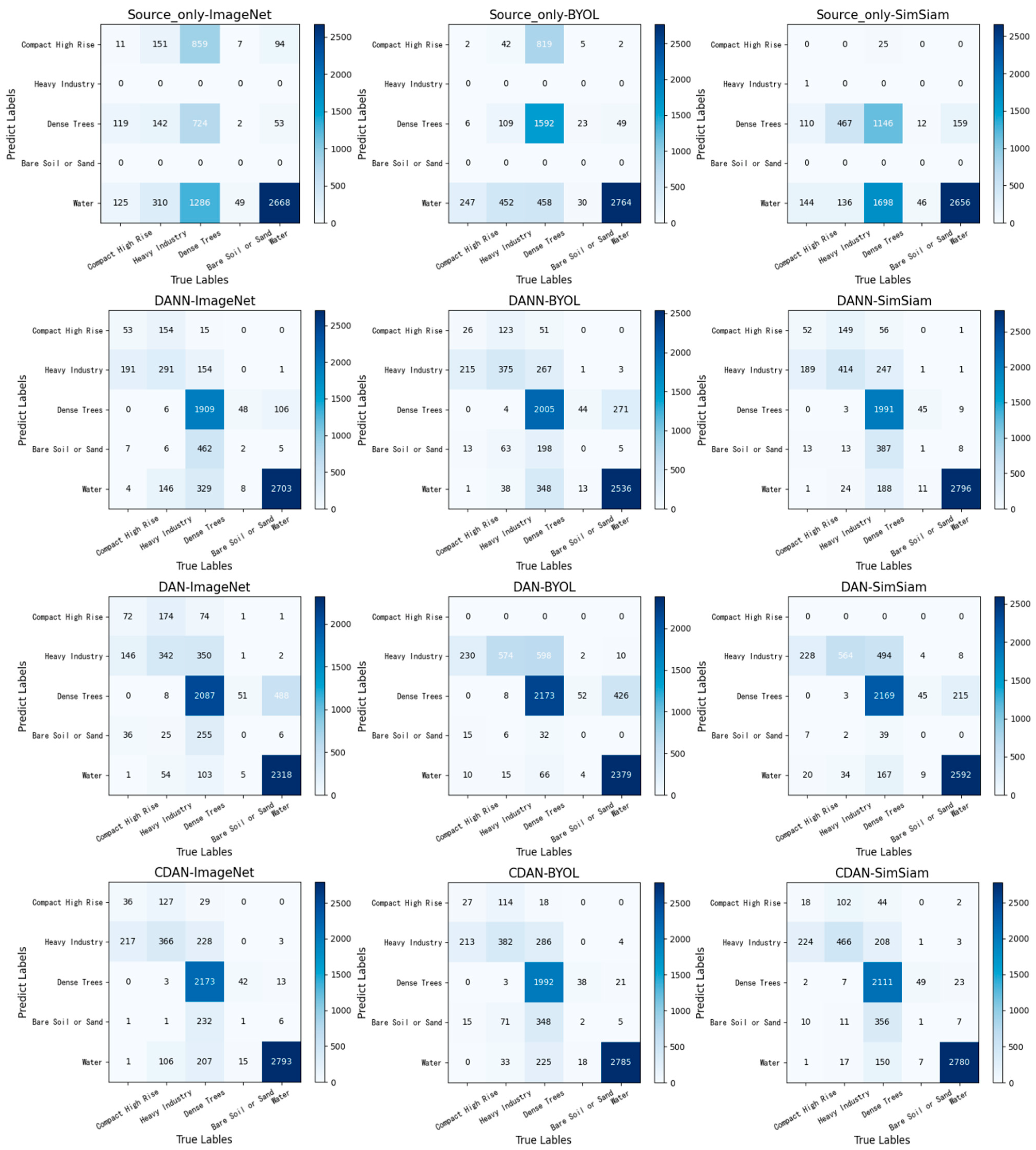
4.4. Transfer Task of Optical to SAR Images
5. Conclusions
Author Contributions
Funding
Data Availability Statement
Conflicts of Interest
References
- Robinson, C.; Malkin, K.; Jojic, N.; Chen, H.; Qin, R.; Xiao, C.; Schmitt, M.; Ghamisi, P.; Hänsch, R.; Hänsch, N. Global land-cover mapping with weak supervision: Outcome of the 2020 IEEE GRSS data fusion contest. IEEE J. Sel. Top. Appl. Earth Obs. Remote Sens. 2021, 14, 3185–3199. [Google Scholar] [CrossRef]
- Chi, M.; Plaza, A.; Benediktsson, J.A.; Sun, Z.; Shen, J.; Zhu, Y. Big data for remote sensing: Challenges and opportunities. Proc. IEEE 2016, 104, 2207–2219. [Google Scholar] [CrossRef]
- Ghamisi, P.; Rasti, B.; Yokoya, N.; Wang, Q.; Hofle, B.; Bruzzone, L.; Bovolo, F.; Chi, M.; Anders, K.; Gloaguen, R.; et al. Multisource and multitemporal data fusion in remote sensing: A comprehensive review of the state of the art. IEEE Geosci. Remote Sens. Mag. 2019, 7, 6–39. [Google Scholar] [CrossRef]
- Li, X.; Lei, L.; Sun, Y.; Li, M.; Kuang, G. Multimodal Bilinear Fusion Network With Second-Order Attention-Based Channel Selection for Land Cover Classification. IEEE J. Sel. Top. Appl. Earth Obs. Remote Sens. 2020, 13, 1011–1026. [Google Scholar] [CrossRef]
- Tuia, D.; Volpi, M.; Trolliet, M.; Camps-Valls, G. Semisupervised Manifold Alignment of Multimodal Remote Sensing Images. IEEE Trans. Geosci. Remote Sens. 2014, 52, 7708–7720. [Google Scholar] [CrossRef]
- Penatti, O.; Nogueira, K.; dos Santos, J.A. Do deep features generalize from everyday objects to remote sensing and aerial scenes domains? In Proceedings of the 2015 IEEE Conference on Computer Vision and Pattern Recognition Workshops (CVPRW), Boston, MA, USA, 7–12 June 2015; pp. 44–51. [Google Scholar]
- Yi, W.; Zeng, Y.; Yuan, Z. Fusion of GF-3 SAR and optical images based on the nonsubsampled contourlet transform. Acta Opt. Sin. 2018, 38, 76–85. [Google Scholar]
- Feng, Q.; Yang, J.; Zhu, D.; Liu, J.; Guo, H.; Bayartungalag, B.; Li, B. Integrating Multitemporal Sentinel-1/2 Data for Coastal Land Cover Classification Using a Multibranch Convolutional Neural Network: A Case of the Yellow River Delta. Remote Sens. 2019, 11, 1006. [Google Scholar] [CrossRef]
- Wang, D.; Du, B.; Zhang, L. Fully contextual network for hyperspectral scene parsing. IEEE Trans. Geosci. Remote Sens. 2021, 60, 1–16. [Google Scholar] [CrossRef]
- Kim, S.; Song, W.-J.; Kim, S.-H. Double Weight-Based SAR and Infrared Sensor Fusion for Automatic Ground Target Recognition with Deep Learning. Remote Sens. 2018, 10, 72. [Google Scholar] [CrossRef]
- Zhuang, F.; Qi, Z.; Duan, K.; Xi, D.; Zhu, Y.; Zhu, H.; Xiong, H.; He, Q. A comprehensive survey on transfer learning. Proc. IEEE 2020, 109, 43–76. [Google Scholar] [CrossRef]
- Cheng, G.; Han, J.; Lu, X. Remote sensing image scene classification: Benchmark and state of the art. Proc. IEEE 2017, 105, 1865–1883. [Google Scholar] [CrossRef] [Green Version]
- Russakovsky, O.; Deng, J.; Su, H.; Krause, J.; Satheesh, S.; Ma, S.; Huang, Z.; Karpathy, A.; Karpathy, A.; Bernstein, M.S.; et al. Imagenet large scale visual recognition challenge. Int. J. Comput. Vis. 2015, 115, 211–252. [Google Scholar] [CrossRef]
- Zhou, H.Y.; Yu, S.; Bian, C.; Hu, Y.; Ma, K.; Zheng, Y. Comparing to learn: Surpassing imagenet pretraining on radiographs by comparing image representations. In Proceedings of the International Conference on Medical Image Computing and Computer-Assisted Intervention (MICCAI), Lima, Peru, 4–8 October 2020. [Google Scholar]
- He, K.; Zhang, X.; Ren, S.; Sun, J. Deep residual learning for image recognition. In Proceedings of the IEEE Conference on Computer Vision and Pattern Recognition, Las Vegas, NV, USA, 27–30 June 2016; pp. 770–778. [Google Scholar]
- Wang, D.; Zhang, J.; Du, B.; Xia, G.S.; Tao, D. An Empirical Study of Remote Sensing Pretraining. arXiv 2022, arXiv:2204.02825. [Google Scholar] [CrossRef]
- Stojnic, V.; Risojevic, V. Self-supervised learning of remote sensing scene representations using contrastive multiview coding. In Proceedings of the IEEE/CVF Conference on Computer Vision and Pattern Recognition, Nashville, TN, USA, 19–25 June 2021; pp. 1182–1191. [Google Scholar]
- Kriegeskorte, N. Deep neural networks: A new framework for modelling biological vision and brain information processing. Annu. Rev. Vis. Sci. 2015, 1, 417–446. [Google Scholar] [CrossRef]
- Geirhos, R.; Rubisch, P.; Michaelis, C.; Bethge, M.; Wichmann, F.A.; Brendel, W. ImageNet-trained CNNs are biased towards texture; increasing shape bias improves accuracy and robustness. arXiv 2018, arXiv:1811.12231. [Google Scholar]
- Albuquerque, I.; Naik, N.; Li, J.; Keskar, N.; Socher, R. Improving out-of-distribution generalization via multi-task self-supervised pretraining. arXiv 2020, arXiv:2003.13525. [Google Scholar]
- Scheibenreif, L.; Hanna, J.; Mommert, M.; Borth, D. Self-Supervised Vision Transformers for Land-Cover Segmentation and Classification. In Proceedings of the IEEE/CVF Conference on Computer Vision and Pattern Recognition, New Orleans, LA, USA, 19–20 June 2022; pp. 1422–1431. [Google Scholar]
- Stojnic, V.; Risojevic, V. Evaluation of Split-Brain Autoencoders for High-Resolution Remote Sensing Scene Classification. In Proceedings of the 2018 International Symposium ELMAR, Zadar, Croatia, 16–19 September 2018; pp. 67–70. [Google Scholar]
- Gómez-Chova, L.; Tuia, D.; Moser, G.; Camps-Valls, G. Multimodal classification of remote sensing images: A review and future directions. Proc. IEEE 2015, 103, 1560–1584. [Google Scholar] [CrossRef]
- Sun, Z.; Dai, M.; Leng, X.; Lei, Y.; Xiong, B.; Ji, K.; Kuang, G. An anchor-free detection method for ship targets in high-resolution SAR images. IEEE J. Sel. Top. Appl. Earth Obs. Remote Sens. 2021, 14, 7799–7816. [Google Scholar] [CrossRef]
- Goyal, P.; Mahajan, D.; Gupta, A.; Misra, I. Scaling and benchmarking self-supervised visual representation learning. In Proceedings of the IEEE/CVF International Conference on Computer Vision, Seoul, Korea, 20–26 October 2019; pp. 6391–6400. [Google Scholar]
- Liu, X.; Zhang, F.; Hou, Z.; Mian, L.; Wang, Z.; Zhang, J.; Tang, J. Self-supervised learning: Generative or contrastive. IEEE Trans. Knowl. Data Eng. 2021. [Google Scholar] [CrossRef]
- Jaiswal, A.; Babu, A.R.; Zadeh, M.Z.; Banerjee, D.; Makedon, F. A survey on contrastive self-supervised learning. Technologies 2020, 9, 2. [Google Scholar] [CrossRef]
- Manas, O.; Lacoste, A.; Giró-i-Nieto, X.; Vazquez, D.; Rodriguez, P. Seasonal contrast: Unsupervised pre-training from uncurated remote sensing data. In Proceedings of the IEEE/CVF International Conference on Computer Vision, Montreal, QC, Canada, 10–17 October 2021; pp. 9414–9423. [Google Scholar]
- He, K.; Fan, H.; Wu, Y.; Xie, S.; Girshick, R. Momentum contrast for unsupervised visual representation learning. In Proceedings of the IEEE/CVF Conference on Computer Vision and Pattern Recognition, Seattle, WA, USA, 13–19 June 2020; pp. 9729–9738. [Google Scholar]
- Chen, T.; Kornblith, S.; Norouzi, M.; Hinton, G. A simple framework for contrastive learning of visual representations. In Proceedings of the IEEE Conference on Computer Vision and Pattern Recognition (CVPR), Seattle, WA, USA, 13–19 June 2020; pp. 2574–2582. [Google Scholar]
- Tian, Y.; Krishnan, D.; Isola, P. Contrastive Multiview Coding. arXiv 2019, arXiv:1906.05849. [Google Scholar]
- Grill, J.B.; Strub, F.; Altché, F.; Tallec, C.; Richemond, P.; Buchatskaya, E.; Doersch, C.; Pires, B.A.; Guo, Z.D.; Azar, M.G.; et al. Bootstrap your own latent-a new approach to self-supervised learning. Adv. Neural Inf. Process. Syst. 2020, 33, 21271–21284. [Google Scholar]
- Chen, X.; He, K. Exploring simple siamese representation learning. In Proceedings of the IEEE/CVF Conference on Computer Vision and Pattern Recognition, Nashville, TN, USA, 20–25 June 2021; pp. 15750–15758. [Google Scholar]
- Bachman, P.; Hjelm, R.D.; Buchwalter, W. Learning representations by maximizing mutual information across views. In Proceedings of the Advances in Neural Information Processing Systems, Vancouver, BC, Canada, 8–14 December 2019. [Google Scholar]
- Ganin, Y.; Ustinova, E.; Ajakan, H.; Germain, P.; Larochelle, H.; Laviolette, F.; Marchand, M.; Lempitsky, V. Domain-adversarial training of neural networks. J. Mach. Learn. Res. 2016, 17, 2096-2030. [Google Scholar]
- Long, M.; Cao, Y.; Cao, Z.; Wang, J.; Jordan, M.I. Transferable representation learning with deep adaptation networks. IEEE Trans. Pattern Anal. Mach. Intell. 2018, 41, 3071–3085. [Google Scholar] [CrossRef]
- Long, M.; Cao, Z.; Wang, J.; Jordan, M.I. Conditional adversarial domain adaptation. In Proceedings of the Advances in Neural Information Processing Systems, Montreal, QC, Canada, 3–8 December 2018. [Google Scholar]
- Scheibenreif, L.; Mommert, M.; Borth, D. Contrastive self-supervised data fusion for satellite imagery. ISPRS Ann. Photogramm. Remote Sens. Spat. Inf. Sci. 2022, 3, 705–711. [Google Scholar] [CrossRef]
- Ioffe, S.; Szegedy, C. Batch normalization: Accelerating deep network training by reducing internal covariate shift. In Proceedings of the International Conference on Machine Learning (PMLR), Lille, France, 7–9 July 2015; pp. 448–456. [Google Scholar]
- Bottou, L. Large-scale machine learning with stochastic gradient descent. In Proceedings of the COMPSTAT’2010, Paris, France, 22–27 August 2010; pp. 177–186. [Google Scholar]
- Deng, W.; Zhao, L.; Kuang, G.; Hu, D.; Pietikäinen, M.; Liu, L. Deep Ladder-Suppression Network for Unsupervised Domain Adaptation. IEEE Trans. Cybern. 2021, 1–15. [Google Scholar] [CrossRef]
- Zhu, X.X.; Hu, J.; Qiu, C.; Shi, Y.; Kang, J.; Mou, L.; Wang, Y.; Huang, R.; Li, H.; Sun, Y.; et al. So2Sat LCZ42: A benchmark data set for the classification of global local climate zones [Software and Data Sets]. IEEE Geosci. Remote Sens. Mag. 2020, 8, 76–89. [Google Scholar] [CrossRef]
- Schmitt, M.; Hughes, L.H.; Zhu, X.X. The SEN1-2 dataset for deep learning in SAR-optical data fusion. arXiv 2018, arXiv:1807.01569. [Google Scholar] [CrossRef]
- Huang, M.; Xu, Y.; Qian, L.; Shi, W.; Zhang, Y.; Bao, W.; Wang, N.; Liu, X.J.; Xiang, X. The QXS-SAROPT dataset for deep learning in SAR-optical data fusion. arXiv 2021, arXiv:2103.08259. [Google Scholar]
- Yang, Y.; Newsam, S. Bag-of-visual-words and spatial extensions for land-use classification. In Proceedings of the 18th SIGSPATIAL International Conference on Advances in Geographic Information Systems, San Jose, CA, USA, 2–5 November 2010; pp. 270–279. [Google Scholar]
- Xia, G.S.; Hu, J.; Hu, F.; Shi, B.; Bai, X.; Zhong, Y.; Zhang, L.; Lu, X. AID: A benchmark data set for performance evaluation of aerial scene classification. IEEE Trans. Geosci. Remote Sens. 2017, 55, 3965–3981. [Google Scholar] [CrossRef]
- Zhao, J.; Zhang, Z.; Yao, W.; Datcu, M.; Xiong, H.; Yu, W. OpenSARUrban: A Sentinel-1 SAR image dataset for urban interpretation. IEEE J. Sel. Top. Appl. Earth Obs. Remote Sens. 2020, 13, 187–203. [Google Scholar] [CrossRef]
- da Costa, V.G.T.; Fini, E.; Nabi, M.; Sebe, N.; Ricci, E. Solo-learn: A Library of Self-supervised Methods for Visual Representation Learning. J. Mach. Learn. Res. 2022, 23, 1–6. [Google Scholar]


| Method | Test Data | ||
|---|---|---|---|
| So2Sat LCZ42-SAR | So2Sat LCZ42-OPT | ||
| Single-source without negative samples | BYOL-SAR | 79.44% | - |
| BYOL-OPT | - | 91.62% | |
| SimSiam-SAR | 73.85% | - | |
| SimSiam-OPT | - | 86.23% | |
| Single-source with negative samples | SimCLR-SAR | 77.23% | - |
| SimCLR-OPT | - | 86.71% | |
| MOCO-SAR | 74.43% | - | |
| MOCO-OPT | - | 86.51% | |
| Multi-source with negative samples | CMC | 74.03% | 87.09% |
| Multi-source without negative samples | Multi-source-BYOL | 81.22% | 92.37% |
| Multi-source -SimSiam | 80.52% | 91.04% | |
| ImageNet | 72.95% | 84.61% | |
| Supervised | 73.71% | 86.16% | |
| Methods | MOCO | SimCLR | CMC | BYOL | SimSiam | ||
|---|---|---|---|---|---|---|---|
| Single-Source | Multi-Source | Single-Source | Multi-Source | ||||
| Upstream CSSL training time | 3 h 37 m | 3 h 05 m | 3 h 17 m | 4 h 12 m | 4 h 13 m | 4 h 12 m | 4 h 14 m |
| Downstream linear classification time | 1 m 17 s | 1 m 17 s | 1 m 17 s | 1 m 17 s | 1 m 17 s | 1 m 17 s | 1 m 17 s |
| Finetuning Initialization | Test Data | ||||
|---|---|---|---|---|---|
| So2Sat LCZ42-RGB | So2Sat LCZ42-SAR | OpenSAR-Urban | UCMerced_LandUse | AID | |
| BYOL-QXS-SARPORT | 94.02 | 81.15 | 57.35 | 93.33 | 95.75 |
| SimSiam-QXS-SARPORT | 92.38 | 81.69 | 51.13 | 83.33 | 88.92 |
| BYOL-SEN1-2 | 92.73 | 81.27 | 48.52 | 63.33 | 83.96 |
| SimSiam -SEN1-2 | 92.83 | 81.49 | 48.70 | 64.17 | 83.73 |
| BYOL-So2Sat LCZ42 | 93.25 | 81.22 | 53.35 | 86.67 | 90.57 |
| SimSiam-So2Sat LCZ42 | 93.15 | 81.21 | 53.40 | 88.00 | 91.98 |
| ImageNet | 92.58 | 80.64 | 59.07 | 97.50 | 95.87 |
| Supervised | 92.74 | 81.09 | 58.58 | 79.17 | 90.80 |
| Initialization Networks | Transfer Methods | |||
|---|---|---|---|---|
| Source-Only | DANN | DAN | CDAN | |
| BYOL | 66.04 | 74.88 | 77.67 | 78.60 |
| SIMSIAM | 57.61 | 79.58 | 80.67 | 81.45 |
| ImageNet | 51.56 | 75.12 | 73.03 | 81.35 |
Publisher’s Note: MDPI stays neutral with regard to jurisdictional claims in published maps and institutional affiliations. |
© 2022 by the authors. Licensee MDPI, Basel, Switzerland. This article is an open access article distributed under the terms and conditions of the Creative Commons Attribution (CC BY) license (https://creativecommons.org/licenses/by/4.0/).
Share and Cite
Liu, C.; Sun, H.; Xu, Y.; Kuang, G. Multi-Source Remote Sensing Pretraining Based on Contrastive Self-Supervised Learning. Remote Sens. 2022, 14, 4632. https://doi.org/10.3390/rs14184632
Liu C, Sun H, Xu Y, Kuang G. Multi-Source Remote Sensing Pretraining Based on Contrastive Self-Supervised Learning. Remote Sensing. 2022; 14(18):4632. https://doi.org/10.3390/rs14184632
Chicago/Turabian StyleLiu, Chenfang, Hao Sun, Yanjie Xu, and Gangyao Kuang. 2022. "Multi-Source Remote Sensing Pretraining Based on Contrastive Self-Supervised Learning" Remote Sensing 14, no. 18: 4632. https://doi.org/10.3390/rs14184632