Article

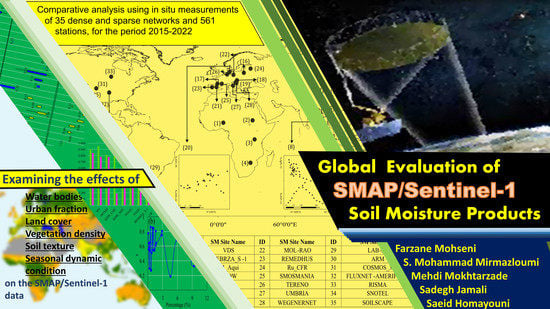
Global Evaluation of SMAP/Sentinel-1 Soil Moisture Products

by
Farzane Mohseni
1,2,*,
S. Mohammad Mirmazloumi
3,
Mehdi Mokhtarzade
1,
Sadegh Jamali
2 and
Saeid Homayouni
4
1
Faculty of Geodesy and Geomatics Engineering, K. N. Toosi University of Technology, Tehran 19967-15433, Iran
2
Department of Technology and Society, Faculty of Engineering, Lund University, P.O. Box 118, 221 00 Lund, Sweden
3
Geomatics Research Unit, Centre Tecnològic de Telecomunicacions de Catalunya (CTTC/CERCA), Av. Gauss 7, E-08860 Castelldefels, Barcelona, Spain
4
Centre Eau Terre Environnement, Institut National de la Recherche Scientifique, Quebec City, QC G1K 9A9, Canada
*
Author to whom correspondence should be addressed.
Remote Sens. 2022, 14(18), 4624; https://doi.org/10.3390/rs14184624
Submission received: 20 August 2022 / Revised: 31 August 2022 / Accepted: 12 September 2022 / Published: 16 September 2022
(This article belongs to the Special Issue Remote Sensing in Environmental Modelling)

Abstract

:
SMAP/Sentinel-1 soil moisture is the latest SMAP (Soil Moisture Active Passive) product derived from synergistic utilization of the radiometry observations of SMAP and radar backscattering data of Sentinel-1. This product is the first and only global soil moisture (SM) map at 1 km and 3 km spatial resolutions. In this paper, we evaluated the SMAP/Sentinel-1 SM product from different viewpoints to better understand its quality, advantages, and likely limitations. A comparative analysis of this product and in situ measurements, for the time period March 2015 to January 2022, from 35 dense and sparse SM networks and 561 stations distributed around the world was carried out. We examined the effects of land cover, vegetation fraction, water bodies, urban areas, soil characteristics, and seasonal climatic conditions on the performance of active–passive SMAP/Sentinel-1 in estimating the SM. We also compared the performance metrics of enhanced SMAP (9 km) and SMAP/Sentinel-1 products (3 km) to analyze the effects of the active–passive disaggregation algorithm on various features of the SMAP SM maps. Results showed satisfactory agreement between SMAP/Sentinel-1 and in situ SM measurements for most sites (r values between 0.19 and 0.95 and ub-RMSE between 0.03 and 0.17), especially for dense sites without representativeness errors. Thanks to the vegetation effect correction applied in the active–passive algorithm, the SMAP/Sentinel-1 product had the highest correlation with the reference data in grasslands and croplands. Results also showed that the accuracy of the SMAP/Sentinel-1 SM product in different networks is independent of the presence of water bodies, urban areas, and soil types.

Graphical Abstract

1. Introduction

A Soil Moisture Active Passive (SMAP) satellite mission was launched by the National Aeronautics and Space Administration (NASA) on 31 January 2015, aboard a Delta II rocket [1]. Modeling of SMAP, a derivative of the formulation studies for the Hydrosphere State (Hydros) mission [2], was initiated in 2008 [3], followed by design studies, critical design review, system integration, and test processing in May 2013 [4,5]. The primary objectives of SMAP were to provide global Soil Moisture (SM) maps, Brightness Temperature (TB), topsoil layer moisture, and freeze–thaw state using L-band microwave spectrum observations [6]. SMAP is considered a follow-up of the Soil Moisture and Ocean Salinity (SMOS) [7,8]. However, the main difference between SMAP and SMOS and, of course, the earlier passive satellites, was the equipment of both L-band (1.26 GHz) radar and L-band radiometer instruments [9].
Microwave emission from the top ~5 cm of soil is measured with a SMAP radiometer with a spatial resolution of ~36 km. In addition, the L-band SAR, which is more sensitive to irregularities of vegetation [10], measures backscatter at higher spatial resolution (1–3 km) [11]. Subsequently, radar and radiometer measurements are effectively combined to produce global SM maps at two higher spatial resolutions: 3 km and 9 km [11,12,13,14]. Thus, the developed algorithms for the SMAP observations promised a unique means of measuring SM with unprecedented accuracy, resolution, and coverage. Unfortunately, due to an unrecoverable hardware failure, SMAP’s radar instrument was discontinued on 7 July 2015, after about 11 weeks of operation [11], and SMAP’s radiometer remains the only operating instrument onboard the satellite. Therefore, this satellite lost its ability to measure the surface SM with a spatial resolution of 3 and 9 km [14].
Using the Backus–Gilbert optimal interpolation technique [15], it became possible to enhance the antenna temperature measurements of SMAP radiometer and provide TB and SM products with a higher spatial resolution [16]. Using this technique, the optimal TB of arbitrary locations is calculated using a linear combination of radiometric measurements overlapped in along- and across-scan directions [17]. As such, the TB disaggregates to the new values with a native resolution equal to the 3 dB beamwidth of the radiometer, which is ~9 km for SMAP [5]. The 9 km TB is then converted to the SM using the Mineralogy-Based Soil Dielectric Model (MBSDM), also called the Mironov dielectric model [18,19]. Consequently, in addition to the 36 km products of SMAP SM, there are further improved SMAP SM products with a spatial resolution of 9 km [20].
To date, numerous researchers have studied the accuracy of SMAP SM products across a wide range of geographic regions and climatic and environmental conditions around the world. Several studies compared the potential of SMAP in determining SM values with the performance of earlier passive microwave satellites such as SMOS, AMSR-E, and ASCAT [21,22,23,24,25,26,27,28,29,30,31].
Moreover, given the data of the SMAP Calibration and Validation (Cal/Val) Core Validation Site (CVS), post-launch field campaigns (such as SMAPVEX-16, SMAPVEX19-22), prelaunch field campaigns, and sparse global networks, there is extensive literature quantitatively evaluating global SMAP products at 36 km and 9 km using in situ measurements, model-based SM estimates, and airborne SM observations [22,32,33,34,35,36,37,38]. Most of these studies demonstrated that SMAP outperforms other passive microwave sensors [8,26,37,39,40,41].
SMAP/Sentinel-1 SM is the latest SMAP product developed to map SM with spatial resolutions of 1 km and 3 km and near-global coverage (latitude from −60 to 60 and longitude from −180 to 180) [14]. In this product, 9 km enhanced TB of SMAP are resampled and downscaled to 3 km and 1 km EASE-Grid using Sentinel-1 radar backscattering data, aggregated onto 1 km and 3 km EASE-Grid 2.0 pixels [42]. The corresponding combination of SMAP data and Sentinel-1 measurements is based on the BT-Based Downscaling Algorithm (BTBDA) [43], followed by the Baseline Retrieval Algorithm and the Tau–Omega algorithm used to generate SM [13].
As SM’s first and only long-term global map with spatial resolutions of 1 km and 3 km, SMAP/Sentinel-1 data represent a turning point for measuring SM with RS systems because they have adequate spatial resolution, global coverage, and acceptable coverage repeat time for many applications. As one of the major sources of SM estimation with Earth Observations (EOs), validation of SMAP/Sentinel-1 products was needed to guide the community and provide information on the quality of products under different conditions around the world and at different times. Generally, since the footprint of passive microwave instruments spans over 1000 km2, SMAP estimates of TB and SM are affected by numerous spatially and temporally variable factors, such as topographic, climatic, land factors, and the radiometric calibration of the passive microwave instruments [44]. Even over certain homogeneous regions, the SM retrieval algorithm and downscaling model applied to combine SMAP and Sentinel-1 data are still influenced by various sources of uncertainty. Satellite instrument noise, model parameterization errors, errors that occur when sampling elliptical footprints onto spatial grids, and imperfections in the retrieval model are some of the most important sources of uncertainty that eliminate the accuracy of SM products [45]. These problems cause the SMAP/Sentinel-1 SM to differ from the true state of SM. Therefore, the comparison of SMAP/Sentinel-1 estimation and the true value of SM illustrates its strength and weakness. So far, few attempts have been made to validate the SMAP/Sentinel-1 SM. Das et al. [46] studied the basic idea and methodology for fusing high-resolution Sentinel-1A/Sentinel-1B data and SMAP products on seven different CVSs. They evaluated the performance of SMAP/Sentinel-1 SM products using in situ measurements of the Walnut Gulch and TxSON sites in the United States, Kenaston in Canada, Monte Buey in Argentina, REMEDHUS and Valencia in Spain, and Yanco in Australia. In addition, Colliander, Reichle et al. (2021) assessed SMAP/Sentinel-1 estimates using the in situ measurements of various CVSs from March 2015 to March 2021. They detailed and investigated the results derived from Monte Buey, Yanco, Kenaston, Valencia, Walnut Gulch, TxSON, Tonzi Ranch in the United States, and HOBE in Denmark.
In line with the previous studies, the focus of this paper is on a global assessment of SMAP/Sentinel-1 SM products using in situ measurements across a wide range of geographic, environmental, and climatic conditions.
The main superiority of this study over the state of the art is the comprehensive evaluation of the performance of the new SMAP/Sentinel-1 SM products on a global scale using in situ measurements from a large number of stations. In this paper, we validate SMAP/Sentinel-1 SM observations using in situ measurements of 561 worldwide stations from 35 SM networks (13 in Europe, 7 in the Americas, 8 in Asia, 4 in Africa, 2 in Australia, and 1 in Oceania). From 31 March 2015 to 1 January 2022, SMAP/Sentinel-1 SM products and in situ measurements were used in this study to analyze the performance of SMAP from the beginning of the mission to the present.
As another innovation in validating the SMAP/Sentinel-1 products, we examine several factors that influence the radiometer and radar observations and the downscaling methods. We compare in situ measurements and SMAP/Sentinel-1 data separately for different seasons, land covers, vegetation densities, and climate zones. We also compare the accuracy of enhanced 9 km SMAP SM products and SMAP/Sentinel-1 data in dense networks to explore to what extent downscaling of SMAP using Sentinel-1 data preserves the accuracy of the source data. It can be said that this study focuses on the qualification of uncertainties in the SMAP/Sentinel-1 product and the comparison of this product with in situ or other suitable reference data across multiple regions and time periods. Consequently, our specific objectives are: (i) long-term evaluation of the SMAP/Sentinel-1 SM across the SM networks around the world, (ii) comprehensive investigation of the effect of various parameters such as land/vegetation cover, water bodies, climate conditions, etc., on the accuracy of the product, and (iii) comparing the SMAP/Sentinel-1 SM with the 9 km enhanced SMAP SM to explore the downscaling effects. The results of this evaluation, along with the official assessment reports conducted by the SMAP science team, enable researchers to determine what spatial resolution, temporal interval, and accuracy can be expected from SM products of a RS satellite in different vegetation conditions, soil textures, seasonal climates, land cover, etc.

2. Study Area and Data

2.1. Validations Sites

Figure 1 represents the central locations and conventional names of 35 SM sites used to validate the SMAP/Sentinel-1 SM product. The distribution and location of in situ stations of three sites, including CTP_SMTMN, HOBE, and a part of SOILSCAPE sites, are also shown in Figure 1. Measurements from these sites were collected by the International Soil Moisture Network (ISMN) platform and are available through https://ismn.geo.tuwien.ac.at/en/networks/ (accessed on 19 August 2022). ISMN is one of the critical existing platforms that has collected data from various SM sites developed by different organizations and countries [47,48]. From all 72 networks and ~2879 stations available in the ISMN, those that meet the following criteria are selected: (i) relatively long-time intervals (more than one year during SMAP/Sentinel-1 coverage from 31 March 2015 to present), (ii) located away from water bodies and urban areas, (iii) with an acceptable distribution and density of stations, and (iv) recording SM at a depth of 0–10 cm of the ground. Table 1 provides the essential information for the selected sites shown in Figure 1.
In Table 1, No. (1) and No. (2) represent the total number of stations at each site and the number of stations used in this study, respectively. As shown in Figure 1 and Table 1, this study used the SM measurements from a total of 561 stations as reference data to investigate the accuracy of the SMAP/Sentinel-1 SM data. The corresponding stations belong to the 35 dense and sparse networks and are distributed worldwide. Dense networks have high spatial sampling densities with longer deployment durations. According to [11], the distribution of stations in a dense network is such that at least eight stations are within a real footprint of passive microwave sensors (approximately 36 km), five stations are within a 9 km spatial grid cell, and three stations are within a 3 km grid cell. Generally, there are 40 SM dense networks, of which eight sites are dense at 3 km pixel size. Based on the measurements of these dense networks, the accuracy of the SMAP/Sentinel-1 SM products was comprehensively evaluated by the SMAP Cal/Val team, reported in [46,77]. Compared to dense networks, sparse networks distributed globally have greater spatial coverage across various climate regimes and biomes [78]. Although sparse networks do not necessarily meet the condition of distributing stations within a 3 km grid pixel, they have some unique properties that make them efficient for validation studies of EOs [24]. Adequate global coverage, temporally coherent reports, accurate measurements, and easy access are some of the features of sparse networks that present them as essential sources for complementing core validation sites and evaluating various RS-based SM products and methods [24]. Moreover, the number of networks and their sampling stations around the world is large enough to present a comprehensive study of the performance of the SMAP/Sentinel-1 mission in estimating SM.

2.2. Data

2.2.1. SMAP/Sentinel-1 Soil Moisture

Level 2 of the SMAP/Sentinel-1 product is considered for the validation process. L2_ SM _SP or SPL2SMAP_S are the abbreviations for this product. SPL2SMAP_S is derived from the enhanced SMAP L-band (~1.4 GHz) radiometer half-orbit 9 km observations and Copernicus Sentinel-1A/1B C-band (~5.405 GHz) radar measurements [79,80]. SMAP/Sentinel-1 retrieves SM over a wide range of vegetation conditions with a temporal resolution of 12 days (based on Sentinel-1’s repeat cycle) and spatial coverage of 180°W to 180°E and approximately 60°N to 60°S [14] (Table 2). For the validation sites, version 3 of SPL2SMAP_S was downloaded from 2015 to 2022. These products are available at https://search.earthdata.nasa.gov/ (accessed on 19 August 2022). The spatial extent of each SMAP/Sentinel-1 image provided on the global cylindrical EASE-Grid 2.0 is limited by the swath width of Sentinel-1A/1B. The image data are in HDF5 format. SPL2SMAP_S HDF5 files consist of three main groups: (i) SM retrieval data with a spatial resolution of 1 km, (ii) SM retrieval data with a spatial resolution of 3 km, and (iii) metadata fields containing all metadata describing the entire contents of each file. Only the 3 km SM and quality assessment plume closest to the SMAP a.m. data (from 6:00 a.m. descending half orbits) were downloaded to reduce the volume of downloaded data and achieve better agreement between reference measurements and observations from RS.

2.2.2. SMAP Enhanced Soil Moisture

In this study, we examine the performance of SMAP’s 9 km products in estimating SM and compare it with the accuracy of the 3 km SMAP/Sentinel-1 SM. Enhanced SMAP products are 9 km radiometer TB and SM derived from native 36 km SMAP measurements using Backus–Gilbert interpolation [85]. The TBs of the enhanced SMAP are corrected for the presence of water bodies (up to 0.1 fractions) before being utilized in the active–passive SM retrieval algorithm. The SMAP Enhanced L3 Radiometer Global Daily 9 km EASE-Grid Soil Moisture (SPL3SMP_E) is used in this study (Table 2). Since version 3 ended on 27 August 2020 and version 4 then replaced the older version, both version 3 and 4 of these products were used in this study. SPL3SMP_E covers the geographic range from 85.044°N to 85.044°S and 180°E to 180°W. Similar to SPL2SMAP_S, the SM and quality assessment flags were downloaded for all validation sites.

2.2.3. CGLS Land Cover

To assess the impact of land cover type on the accuracy of SMAP SM, we use the Copernicus Global Land Service (CGLS) land-cover product with a spatial resolution of 100 m (CGLSLC100) [86]. Version 3 of the CGLS-LC100 products covers the geographic range from 180°E to 180°W and 78.25°N to 60°S. The CGLSLC100 map includes 22 classes, including six different species of closed forest, six different species of open forest, shrubs herbaceous vegetation, wetland, moss and lichen, sparse vegetation, cropland, urban, snow and ice, permanent water bodies, and open sea. However, this paper examines the effects of eight different land-cover types in the accuracy of SMAP/Sentinel-1 SM: Build-up, Cropland, Forest, Shrubland, Grassland, Bareland, Water, and Wetland. To this end, we reclassified the CGLSLC100 map into the mentioned land-cover classes. Thus, the land cover of closed and open forests, including evergreen needle leaf, deciduous needle leaf, evergreen broad leaf, deciduous broad leaf, and mixed deciduous forest, has been reclassified as forest. In addition, herbaceous vegetation, mosses, and lichens are classified as grassland. Snow and ice, permanent water bodies, and open seas are also reclassified as water. Figure 2 shows the global land cover map of CGLSLC100 for the reference year 2015, downloaded from Google Earth Engine and reclassified to the eight mentioned land-cover classes.

2.2.4. Soil Texture and Vegetation Fraction Map

We used the Harmonized World Soil Database (HWSD) to evaluate the effects of soil properties on the accuracy of SMAP/Sentinel-1 SM. The HWSD is a 30 arc-second grid database consisting of 21,600 rows and 43,200 columns linked to harmonized soil property data [83]. The primary soil information included in the HWSD datasets is organic carbon, pH, water-holding capacity, soil depth, soil cation exchange capacity, clay content, total exchangeable nutrients, lime, and gypsum content, sodium exchange percentage, salinity, texture class, and granulometry. Version 1.0 of the HWSD, released in 2008, has been updated several times with new information and is used extensively around the world. Recently, the HWSD was adopted by the Global Soil Partnership (GSP) as the current authoritative soil database (Table 2).
The multispectral and multiresolution data from Sentinel-2 were used along with the land-cover and soil properties maps to calculate vegetation fraction and NDVI. Similar to Sentinel-1, Sentinel-2 was developed by ESA to provide a multiband dataset over land and coastal waters [84,87]. Depending on the spectral band, the spatial resolution of Sentinel-2 varies from 10 m to 60 m [88]. The red and NIR bands with a spatial resolution of 10 m are used in this study to estimate the monthly and seasonal NDVI.

3. Methodology

According to the quality assurance framework advocated by the Land Product Validation (LPV) subgroup of the Committee on Earth Observation Satellites (CEOS) (https://lpvs.gsfc.nasa.gov/ (accessed on 19 August 2022)), the validation process of SM datasets should be able to provide a reliable quantitative assessment of their systematic and random errors through analytical comparison with reference data [89]. In recent decades, several methods have been developed to validate coarse-scale passive microwave EOs through numerous in situ measurements [11,90,91], airborne campaigns [92,93,94,95], and model-based SM estimates [96,97]. Given data preprocessing, the evaluation strategies, and the applied reference data, the methods cause different uncertainties and ambiguities in validating SM products [98]. To standardize validation practices across EO communities, many efforts have been made to establish comprehensive protocols for validating satellite-based SM maps [89,98,99,100]. Refs [89,101] reviewed the compilation of the most common theoretical considerations for validating EOs and presented a comprehensive protocol for validation practices of satellite SM products. The SMAP/Sentinel-1 SM validation approach used in this work is largely consistent with the recommendations in [101], and was recently used in [77]. Figure 3 schematically shows a workflow of the validation method applied in this study to assess the performance of SMAP/Sentinel-1 active/passive SM data. This validation approach can be divided into the following four steps: (1) selection of reliable reference data, (2) preprocessing of data, (3) application of statistical indicators, and (4) presentation of validation results. All steps contain sub-steps, three of which are discussed in more detail in the following sections. The last step is presented in Section 4 and Section 5 as an outcome of this study.

3.1. Selecting Reliable Reference Data

The validation networks of SM usually provide the reference data at different soil depths from 0–5 cm to 2 m with different sampling intervals, from hourly to monthly collection periods [102]. Those best matching satellite estimates must be selected for the assessment process [103]. Regarding the penetration depth of the microwave portion of the electromagnetic spectrum, which is typically 3 cm [104], SMAP/Sentinel-1 products typically estimate the top few centimeters SM of soil [24,104]. Therefore, in the validation networks, out of all SM measurements at different depths (0–5 cm, 10 cm, 20 cm, 50 cm, and 100 cm), the measurement at a depth of 0–5 cm was used for the validation process. In the absence of 0–5 cm measurements, measurements at 0–10 cm depth were used, which correlated with surface SM [105,106]. Those stations that did not have any measurements at depths above 10 cm were masked out. According to Table 1, except for WEGENERNET, UMBRIA, MOL/RAO, KIHS_CMC, and KIHS_SMC, the rest of the sites measure surface SM. SM values of the depth above 10 cm at the mentioned sites were downloaded and applied in the validation process.
To minimize the time gap between the satellite and reference data, the in situ observations closest to the SMAP overflight time (approximately 6:00–7:00 a.m. local time) were used at each validation site. Moreover, of all the selected data, measurements on days with non-zero snow indicators (e.g., snow depth or snow water equivalent) and ground surface or air temperature below 4 °C were excluded from the entire procedure.

3.2. Data Preprocessing

Data preprocessing aims to spatially or temporally align the different data sets coming from various sensors, platforms, and techniques (e.g., coarse-resolution satellite products, modeled data, and field networks). In the evaluating satellite products, when coarsely gridded estimates must be accurately compared to point-based in situ measurements [107], data preprocessing is generally an essential step. Depending on the number and type of datasets used in a study, preprocessing and matching between measurements involve several sub-steps, all described in detail in [101]. In this study, the following two preprocessing steps were used:

3.2.1. Masking out Unreliable Pixels

To avoid unreliable data, SMAP/Sentinel-1 SM products were checked through a quality-control procedure to identify and discard unreliable observations, values outside the acceptable range, spikes, and sudden dips. According to [101] recommendation, we discarded all pixels that were at least 20% covered by tropical forests, urban areas, water bodies, and wetlands, as well as all areas with vegetation water content greater than 5 kg/m2 and NDVI greater than 0.7. In addition, the data flags of the SMAP/Sentinel-1 products were used to identify and eliminate data that were not recommended. Data flags are typically placed on non-recommended targets for various reasons, including inappropriate locations for querying SM, unreliable measurements TB, and faulty algorithms for querying SM.

3.2.2. Calculating Reference SM within the Grid Pixels

All stationary in situ measurements within a particular grid cell were averaged to make the RS pixel-based data as representative as possible [108]. There is a sizeable spatial discrepancy between the point-based reference measurements and the grid-based satellite observations [109]. To this end, the weighted average of stations located within a SMAP/Sentinel-1 pixel was calculated at the geographic center of the pixel (Equation (1)).
S M C i n s i t u = i = 1 n P i × S M i i = 1 n P i
where n is the number of stations located in a SMAP pixel, and the values SMi and Pi are, respectively, the point measurement of the ith station and its weight, related to the distances to the center of the pixel (Equation (2)).
p i = 1 ( x i x o ) 2 + ( y i y o ) 2
where (xi,yi) and (xo,yo) are the geographic location of the corresponding station and the center of the SMAP pixel. As mentioned earlier, this study evaluates SMAP/Sentinel-1 SM 3 km products using in situ measurements of sparse networks with surrogate stations; therefore, there is no more than one point-based station in most SMAP/Sentinel-1 pixels.

3.3. Statistical Metrics for the Evaluation Process

Previous scientific literature has used various statistical indicators to compare RS data with field observations and to describe the performance of EOs collected by various sensors (e.g., multispectral [110,111], hyperspectral [112], LiDAR [113], thermal [114], and SAR [115]), and platforms (e.g., UAVs and satellites). The underlying concept is that the overall error of an observed/measured value (x) is separable into its systematic (αx and βx) and random (εx) components (Equation (3)).
X = α x + β x t + ε x
Here, εx is an additive mean random error, and αx and βx are additive first-order systematic errors and multiplicative (second-order) errors in the assumed grid cell with average SM (t). Equation (3) can be considered for both RS observations and in situ measurements. εx is assumed to be zero in almost all EOs validation studies for reference and EOs datasets. For the in situ measurements considered in the reference dataset, it is assumed that αx~0 and βx~1. In addition, for the evaluation of EOs, statistical moments are typically estimated in the temporal domain (i.e., temporal mean, variance, and covariance), assuming stationary first- and second-order systematic errors (i.e., means and variances are assumed to be constant over time). Under these assumptions, the performance of a SM product is directly related to its uncertainties, characterized by the actual measurements of the reference data.
Consequently, all validation metrics that assume the behaviors of EOs as a random variable can be computed to investigate the performance of a SM product. Mean Difference (MD), Root Mean Squared Difference (RMSD), and unbiased Root Mean Squared Error (ub-RMSE) are the most common relative metrics used to estimate the uncertainty of EOs. These comparison metrics are commonly used to evaluate coarse-scale SM products obtained from passive RS techniques and instruments [37,116,117]. The MD represents the uncertainty of the variable being evaluated and contains both systematic and random components. In some scientific literature, this parameter is also referred to as bias. Basically, MD measures the difference between the reference measurements from SM and the satellite retrievals from SM (Equation (4)).
MD = ( SM S S M R   ¯ ) = 1 N   i = 1 N ( S M S . i S M R . i )   = 1 N   i = 1 N α SM S . i + ( β SM R . i 1 ) t  
where N is the number of data applied to calculate the statistics, which depends on the number of stations of sites, the number of coarse-scale pixels covering the site’s extent, and the time interval. Vinculums indicate the average of the values. SMS and SMR, respectively, refer to the satellite observation and in situ SM. With SMR as the reference data, MD collapses to 1 N α S M s . i + ( β S M R . i 1 ) t , directly estimating the biases of the satellite retrieval. Note that, given the t phrase, MD is still influenced by the average SM conditions. In addition to MD, RMSD calculates the absolute difference in retrievals from SM relative to reference values using the following equation (Equation (5)):
RMSD = ( S M S S M R   ¯ ) = i = 1 N ( SM S . i S M R . i ) 2   N  
RMSD is more applicable than the RMSE in validating coarse-scale SM products using station-based reference measurements [118]. The main idea behind estimating RMSD instead of RMSE is that the point-based reference value may differ from the actual SM value over a grid cell. Due to the possible errors in the reference values, the RMSD should be used to validate the raster pixels by stationary measurements. In addition, the ub–RMSE metric can provide a more reliable estimate of the RMSD. Unlike the RMSD, which is sensitive to additive and multiplicative biases, the ub–RMSE is only affected by multiplicative biases (Equation (6)).
u b - R M S E = RMSD 2 b SM ( R , S ) 2 = R M S D 2   M D 2
where bSM(R,S) is considered the first-order (additive) bias between reference data and EOs. Therefore, ub–RMSE is a bias-insensitive indicator and refers to the standard deviation of the error. In the sparse network, if a station’s measurement is considered the true SM value of the 3 km SMAP/Sentinel-1 grid cell, MD, RMSD, and ub–RMSE conservatively represent the true values of the corresponding indicators.
In addition to uncertainty-related parameters, parametric and non-parametric correlation methods intensely examine the dependency between two datasets. The statistical correlation value between two datasets is a significant indicator because it shows the detailed data’s signal-to-noise ratios (SNRs). The Pearson correlation coefficient (r) is one of the most common SNR-related relative metrics used to evaluate EOs. Although the correlation coefficient, representing the statistical dependence between the satellite observation and the reference value, can take values between −1 and 1, negative observations were not considered in the validation process. Therefore, the r values closer to 0 indicate a weak correlation between the satellite observation and the SM reference value due to noise and errors in the satellite measurements. The r values closer to 1 indicate a strong relationship between these two data sets.

4. Results

4.1. SMAP/Sentinel-1 Overall Accuracy

Table 3 provides additional information on the validation sites—including the minimum, maximum, and average NDVI and SM values, the number of SMAP/Sentinel-1 product pixels assessed at each site (column 8 of Table 3), the number of pixels with more than one station, the number of stations in the corresponding pixels (the number in the parenthesis in column 9), and the total number of data points used to assess the SMAP/Sentinel-1 products—separately for each site. The number of data points used to validate SMAP/Sentinel-1 is also listed separately for each season in this table.
Table 3 shows that validation sites are found in various vegetation and SM conditions. BIEBRZA_S-1, with an average SM of 0.54, and Ru_CFR, with an average SM of 0.56, are two of the wettest networks available in Europe. The lowest humidity is found in African networks, such as AMMA-CATCH, with an average of SM of 0.037, and SD_DEM, with an average of SM of 0.038. In situ stations were distributed among a total of 440 SMAP/Sentinel-1 pixels, 31 of which have multiple field stations. For this analysis, 88,293 data points were obtained from over three hundred thousand SMAP/Sentinel-1 files and images. This information is evenly distributed across all four seasons: 22,611 data in the spring, 23,294 data in the summer, 23,250 data in the fall, and 19,138 data in the winter.
Figure 4 shows four different estimated statistics as boxplots for all validation sites with a high-quality satellite. It should be noted that since the correlation coefficient between the in situ measurement and satellite data was negative in the HOAL site, the results of this site were not mentioned in Figure 4. In this figure, the results for the different continents are shown in different colors. Using the median, minimum, maximum, and 1/3 quantiles of the analyzed statistics for each site, these plots can provide an overview of the performance of SMAP/Sentinel-1 in estimating SM. For better schematically representation of the results, the global quantitative maps of average correlation coefficient, average RMSD, average MD, and average ub-RMSE of validation sites are shown in Figure 5.
Regarding correlation coefficients (r) (Figure 4a), the highest correlation between SMAP/Sentinel-1 observations and in situ measurements is founded on SOILSCAPE (average r value of 0.86) with 30 ground stations distributed across the United States. Some stations at this site and some stations at other sites in Africa and North America have correlation coefficients greater than 0.95. FR_Aqui follows SOILSCAPE in Europe with an average r of 0.85 and AMMA-CATCH with an average r of 0.84. On the other hand, the LAB-net with four stations has the lowest correlation coefficient (average r of 0.17). Following this network, the lowest correlation coefficients are found in KIHS_CMC (average r of 0.19), 18 SMAP/Sentinel-1 grid cell stations, and IPE (average r of 0.27).
Based on the RMSD values of the different sites (Figure 4b), it can be seen that in most networks, the normal difference between in situ measurements and SMAP/Sentinel-1 SM observations is greater than 0.1. The highest RMSD values are observed in BIEBRZA_S-1 and Ru_CFR sites with two stations, with an average RMSD of 0.3 and 0.33, respectively. The lowest RMSD values are founded on SD_DEM and COSMOS-1 in Asia and NGARI in Africa. Regarding MD values (Figure 4c), the worst results (corresponding to the largest MD values) were again obtained at the BIEBRZA_S-1 and Ru_CFR sites, confirming previous results. MD values at other sites ranged from −0.2 for LAB-net to 0.12 for KIHS_CMC. However, despite high RMSD and MD errors at some sites such as BIEBRZA_S-1, Lab-net, and Ru_CFR, the ub–RMSEs of these sites (Figure 4d) are acceptable and comparable to those of other networks. In general, ub–RMSE ranges from 0.03 for SD_DEM and NGARI to 0.16 for COSMOS-2. It can be seen that the ub–RMSE values of four sites, three of which are in Africa and one of which is in Asia, meet the nominal error (RMSE better than 0.04 m3/m3) of the SMAP mission. With an average r of 0.78 and a ub–RMSE of 0.05, Oceania shows the best results validating SMAP/Sentinel-1 SM products. Africa follows Oceania with an average r of 0.71 and an ub–RMSE of 0.045.

4.2. Comparison of SMAP/Sentinel-1 and Enhanced SMAP SM Products

Figure 6 shows a schematic summary of the number and percentage of available SMAP 9 km and SMAP 3 km images for the validation sites. The numbers in parentheses represent the actual temporal resolution of the SMAP/Sentinel-1 and enhanced SMAP products. The revisit time is calculated based on the number of data available at each site and their availability period (see Table 1), taking into account the SMAP/Sentinel-1 data gap, which is given in https://nsidc.org/data/SPL2SMAP_S/versions/3 (accessed on 19 August 2022).
In terms of data accessibility over the same period, the superior performance of SMAP 9 km products compared to SMAP/Sentinel-1 data is evident in Figure 6. In most parts of the world (e.g., Asia, Australia, Africa, and the Americas), the total number of SMAP/Sentinel-1 images is almost half of the total number of enhanced SMAP products. Moreover, the average actual revisit time of enhanced SMAP is 2 days, while SMAP/Sentinel-1 has an average revisit time of 6 days. Figure 7 shows the overall results for the performance of the enhanced SMAP and SMAP/Sentinel-1 products in terms of the four metrics: correlation coefficient (r), RMSD, bias, and ub–RMSE. Note that this figure includes results for validation sites where both SMAP/Sentinel-1 and enhanced SMAP products have grid cells within more than one station. The last columns of each graph in Figure 7 show the average values of the corresponding metrics.
Regarding correlation coefficient values (Figure 7a), the correlation coefficient ranges from 0.18 for the WEGENERNET site to 0.95 for the PTSMN site with enhanced SMAP products and from 0.189 for the KIHS_CMC site to 0.84 for the AMMA-CATCH site with SMAP/Sentinel-1 products. At almost all validation sites except WEGENERNET, higher r values were estimated for enhanced SMAP products at 9 km spatial resolution. The difference between the r values, obtained for SMAP/Sentinel-1 and enhanced SMAP data, is larger for some networks, such as KIHS_CMC and KIHS_SMC, and smaller for some sites, such as Ru_CRF, HOBE, and RISMA. Figure 7a shows that the enhanced SMAP product, with an average r of 0.83, outperforms the SMAP/Sentinel-1 product, which has an average r of 0.6, in estimating SM. Moreover, in almost all networks, the RMSD of the SMAP/Sentinel-1 products (with an average of 0.15) is larger than that of the enhanced SMAP products (with an average of 0.11) (Figure 7b). As noted above, the RMSD value is a function of representativeness error, SMAP reference error in estimating TB and the SM retrieving method, and uncertainties in the BTBDA downscaling algorithm and Sentinel-1 backscatter measurements. Therefore, Figure 7b implies that a portion of the error (average value of 0.04) is imposed on the SM observations after using the Sentinel-1 backscatter measurements and downscaling method. In all networks except BIEBRZA_S-1 and Ru_CFR, RMSD is between 0.06 and 0.17. The RMSD values of BIEBRZA_S-1 and Ru_CFR are abnormally high for SMAP 9 km and SMAP/Sentinel-1. Figure 7c shows the same result for these two sites, with substantial negative bias values for both products. This confirms that the very high values obtained in RMSD of BIEBRZA_S-1 and Ru_CFR are not due to satellite observation error. Instead, a large part of the values is a result of representativeness error. Given the ub–RMSEs of enhanced SMAP calculated for each site (Figure 7d), removing the biases from the RMSDs brings the error of almost all validation sites closer to the SMAP nominated error, 0.04 m3/m3. However, high ub–RMSEs in BIEBRZA_S-1 and Ru_CFR sites cause the average error to be 0.074. By deleting the information of these two networks, the average ub–RMSE is reduced to 0.065. On the other hand, ub–RMSEs for the SMAP/Sentinel-1 were generally presented as more than 0.04 m3/m3, as the average of ub–RMSEs of all sites is ~0.093.

4.3. Impacts of Vegetation Conditions, Land Cover, and Soil Texture on the Accuracy of SMAP/Sentinel-1 SM Products

To investigate the influence of land cover on the accuracy of SMAP/Sentinel-1 SM products, the statistical indicators were calculated for different land covers of the validation sites. For this purpose, the land-cover class that accounts for more than 70% of the study area is considered the validation site’s mainland cover. Regions equally covered by forest and grass are assigned to the “Forest + Grassland” class. In this way, the regions covered by forest and cropland are considered the “Forest + Cropland”. Figure 8 illustrates the effects of land cover on the accuracy of SMAP/Sentinel-1 SM products.
The SMAP/Sentinel-1 observations in Grassland have the highest correlation coefficient (average r of 0.701) with the in situ measurements. After Grassland, the correlation coefficient obtained the best results in the Cropland (average r of 0.651) and Forest + Cropland (average r of 0.613) classes. However, the lowest error (average RMSD and ub–RMSE values) are observed in Bareland regions (average RMSD = 0.06 and un-RMSE = 0.030). According to Figure 8, the error values are higher in Cropland (average RMSD = 0.115 and un-RMSE = 0.083) and Grassland (average RMSD = 0.113 and un-RMSE = 0.077) compared to the Bareland. On the other hand, SMAP/Sentinel-1 SM products showed poor results in the correlation coefficient, RMSD, and ub–RMSE in the Forest regions (R = 0.434, RMSD = 0.161, and ub–RMSE = 0.106). It can also be seen that the presence of forests in the grassland regions affects the accuracy of the SMAP/Sentinel-1 products (Grassland versus Forest + Grassland in Figure 8). These results show less sensitivity of the SMAP/Sentinel-1 to SM content variations beneath vegetation, especially in very moist vegetation and forest regions.
We also investigate whether water bodies and urban areas less than 0.25 km2 that are not detectable in the MODIS land-cover products can affect the accuracy of the SMAP/Sentinel-1 SM products. The underlying concept is that the MODIS land-cover product with a spatial resolution of 500 m and 1 km is used as dynamic ancillary data to eliminate the influence of water bodies, building areas, woodlands, and croplands on both the active–passive algorithm [46] and the SM retrieval algorithm of TB [13]. The results of this assessment are shown in Figure 9. The plots (a) and (b) in Figure 9 show the relationship between the percentage of water/urban classes within the validation regions and the correlation coefficient obtained between the SMAP/Sentinel-1 SM observations and the in situ measurements. The same results for the RMSD are shown in the plots of (c) and (d) in Figure 9. Note that to better examine the impact of water bodies on SMAP/Sentinel-1 performance, we have considered the wetland as a water body in this part of the validation process.
According to Figure 9, the highest percentage of water bodies and urban areas in the validation sites were a maximum of 7% and 12%, respectively. Figure 9 shows that for those pixels of SMAP that include water bodies and urban areas, after MODIS land-cover correction, the accuracy of the SMAP/Sentinel-1 SM product is independent of the presence of water bodies and urban areas. It can be concluded that the corrections applied in the 3 km products of SM using the MODIS land-cover map with a spatial resolution of 500–1000 m were able to minimize the effects of water bodies on the dielectric constant extracted for L-band radiometry and the effects of the urban area on the backscatter coefficient retrieved by the Sentinel-1 radar instrument.
The representation in Figure 10 shows the overall accuracy of the SMAP/Sentinel-1 products at all validation sites as a function of soil type. Figure 10a shows the percentage of validation networks belonging to six different soil types. All soil types have medium or coarse surface textures. According to Figure 10a, 46% of the networks studied have sandy loam soil. After sandy loam, clay and loam soils have the most significant number of networks, with about 23% and 21% of the networks, respectively. Only one network had sandy soils.
Figure 10b,c shows the average correlation coefficient and ub-RMSE of each soil type. Given this figure, the SM measurements of 4% of the networks with sandy clay loam soil have the highest correlation with the SMAP/Sentinel-1 SM products. As can be seen in this figure, despite the slight similarity between the average correlation coefficients and ub-RMSE in the different soil types, it can be said that the influence of the soil type on the accuracy of the results can be ignored.

4.4. Seasonal Assessment of the SMAP/Sentinel-1 Performance

The statistical indicators were calculated for the four seasons for a more in-depth investigation into the dependence of the results shown in Figure 4 and Figure 7 on the seasonal climatic conditions. Figure 11 shows the histogram of r values of validation sites.
The results presented in Figure 11 show that SMAP/Sentinel-1 SM observations in winter have the lowest correlation with in situ measurements. In this season, the correlation coefficients of more than 50% of the validation networks were below 0.5 and even below the average r value of this season (i.e., 0.269). In contrast, in autumn, the correlation between in situ data and retrieval values from SMAP/Sentinel-1 SM is the highest. In this season, the correlation coefficients obtained for more than half of the validation networks range from 0.55 to 1. Thus, with an average value of 0.53, autumn has the best accuracy for estimating SM. Note that despite the significant differences in the histogram obtained in spring and autumn, the average correlation coefficients in these two seasons are not significantly different. Therefore, spring was identified as the second season with average correlation coefficients of 0.51.

5. Discussions

5.1. SMAP/Sentinel-1 Overall Accuracy

The ISMN SM networks provide in situ measurements of SM under a variety of conditions that can be used to validate SMAP/Sentinel-1 SM products. The analysis of SMAP/Sentinel-1 SM data in various validation sites shows that this moderate-resolution SM product can provide SM with acceptable accuracy (Figure 4). Consistent with the pattern of the performance metrics over all sites, dense validation sites, which have a larger number of stations distributed within the SMAP/Sentinel-1 cell, had a higher correlation coefficient and lowered ub–RMSE (Figure 4 and Table 3). According to Figure 4, despite the high correlation coefficient (R) between in situ measurements and SMAP/Sentinel-1 SM observations, there are high RMSD values at some sites such as BIEBRZA_S-1 and Ru_CFR (Figure 4b). However, the high observed bias (Figure 4c) at these two sites indicates that the high RMSD values are due to a possible undetectable and undesirable error, called representativeness error [119,120]. Representativeness error refers to the difference between the real SM value within a particular grid cell, and the average of point-based in situ measurements within the corresponding grid cell considered the reference values [101]. This error is unrelated to satellite performance and must be removed from the validation process. The large bias values between the enhanced SMAP SM observations and the in situ measurements from BIEBRZA_S-1 and Ru_CFR (Figure 7c) can show the representativeness error in these networks. According to Equations (3) and (4), this type of error in the validation process causes α of the reference data to be non-zero, which significantly affects the results, especially at higher SM values. As detailed in Table 3, BIEBRZA_S-1 and Ru_CFR are two of the wettest networks available, and both are located in Europe. Based on the assumptions considered for the validation process of EOs, representativeness error is unavoidable incredibly when coarse-scale SM product is evaluated using sparse or dense SM networks [121]. According to Figure 4c, from all validation sites, 18 sites have a negative bias, 13 sites have a positive bias, and 3 others have zero bias. The bias is not due to an overestimation or underestimation of satellite observations, but a possible representativeness error. Fortunately, this error is detectable using MD and bias and can be decreased from the overall error of the EOs. Therefore, the ub–RMSE, which separates the bias values (MD) from the RMSD, can better explain the performance of SMAP/Sentinel-1. By comparing RMSD and ub–RMSE indicators of the BIEBRZA_S-1 and Ru_CFR sites, it can be seen that the ub–RMSE decreased sharply after removing the MD from the RMSD values. The presence of good correlations (Figure 4a) in these two networks also confirms that the observed error is not related to satellite performance. Similar performance (SM retrievals without significant errors) have also been found and reported for previous SM products retrieved from various RS missions, such as SMOS, AMSR_2/E, and SMAP coarse-scale SM products [24]. Compared with coarse-scale SM products divided from previous passive microwave satellites, the SMAP/Sentinel-1 product with a higher spatial resolution can therefore be more beneficial for various purposes.

5.2. Comparison of SMAP/Sentinel-1 and Enhanced SMAP SM Products

Figure 6 and Figure 7 compare the performance of SMAP/Sentinel-1 and enhance SMAP from different points of view. The underlying concept is that for the derivation of SMAP/Sentinel-1 SM product, enhanced SMAP L-band radiometer observations from half orbit are used as a reference radiometer measurement and downscaled with Sentinel-1 radar data [19]. Comparison of SMAP-9 km and SMAP/Sentinel-1 3 km SM products allowed us to determine the magnitude of the error imposed on SMAP-3 km SM by the SMAP-9 km reference data, Sentinel-1 backscattering measurement, or BTBDA downscaling method. Moreover, it expressed the negative effects of integration of Sentinel-1 and SMAP data on the various characteristics of SMAP original products (e.g., its temporal resolution (Figure 6). As shown in Figure 6, the actual revisit time of the enhanced SMAP is twice as long as that of SMAP/Sentinel-1. Therefore, in terms of data availability over the same period, the SMAP 9 km products are superior to the SMAP/Sentinel-1 data. This result could be partly explained by the low revisit time of the Sentinel-1A/B satellites. In short, the studies conducted before the launch of the SMOS mission showed that an interval of 2–3 days is the optimal temporal resolution for a passive microwave mission SM [122]. In this way, as a follow of the SMOS mission, the nominal revisit time of SMAP is planned for 2–3 days [19,123]. However, in the case of SMAP/Sentinel-1, temporal resolution is limited by the Sentinel-1A/B satellites’ revisit time (~six days) [14]. Moreover, since the Sentinel-1B satellite is no longer available, the repeat coverage of radar data may worsen. In addition to the low revisit time of the Sentinel-1A/B satellites, the active–passive SMAP algorithm, which discards any suspect or erroneous backscatter coefficient, reduces the revisit time of the SMAP/Sentinel-1 product.
Given Figure 7a–d, the enhanced SMAP product has better performance when it comes to estimating SM than the SMAP/Sentinel-1 product. The SMAP/Sentinel-1 development team has attempted to overcome the major challenges of combining active and passive microwave measurements by considering (i) temporal mismatch between the two independent satellite platforms SMAP and Sentinel-1A/B, (ii) estimation of different beta and gamma parameters (the coefficient of the linear functional relationship between backscatter coefficient and TB), and (iii) different frequencies and penetration depths of the active and passive instruments. By comparing the results obtained from the evaluation of SMAP/Sentinel-1 products with the validation results for previous active–passive algorithms, it can be seen that they have been successful in achieving their goals. However, given the conditions and assumptions applied to the integration of the enhanced SMAP and Sentinel-1 data, and the inherent inaccuracies of the radar data due to the influence of target structure and vegetation condition, this conclusion is to be expected [124]. It must be kept in mind that, despite the differences in the performances between SMAP-enhanced and SMAP/Sentinel-1 data, these high-resolution SM products still meet the demand for overall accuracy in estimating SM.

5.3. Impacts of Various Geographical Parameters on the Accuracy of SMAP/Sentinel-1 SM Products

Based on Figure 8, the performance metrics over the non-forested sites were significantly better than the level achieved in the woodland areas. Minimal sensitivity to incident angle variations of SMAP radiometer for heavily vegetated areas [77], the sensitivity of Sentinel-1 radar to vegetation roughness and dispersion [125], masking of incident angle variations of active–passive microwaves by dense vegetation [46], lower penetration of electromagnetic waves in dense vegetation [126,127], and the effect of plant moisture on the dielectric coefficient might be the main reasons for this result. A similar result was obtained by [128], indicating that the accuracy of SMAP SM decreases with decreasing vegetation percentage, especially in the forest areas. On the other hand, Colliander, et al. [129] enhanced SM products with in situ measurements after comparing the observation of SMAP, demonstrates that spaceborne L-band radiometry is sensitive to SM under temperate forest canopies (RMSD range of 0.047–0.057 m3/m3 and r rang of 0.75–0.85). Since the results of this study show the same range of the correlation coefficient for SMAP-enhanced SM products at the forest validation sites (such as KIHS_CMC, SMOSMANIA, and TERENO, Figure 7), the substantial part of the error must be added to the products after combination with active radar data.
It must be noted that vegetation effect correction is considered in both the active–passive algorithm [46] and the SM retrieval algorithm of TB [13] using the MOD13A2 (V005) vegetation indices product [130]. However, due to the remarkable temporal changes in vegetation and surface roughness [12] and the presence of diverse vegetation with different spectral characteristics in a coarsely scaled SMAP pixel [131], the vegetation effect correction might be incomplete in some vegetated areas. The poor performance of the SMAP/Sentinel-1 products in the shrubland (R = 0.510, RMSD = 0.161, and ub–RMSE = 0.106, Figure 8) is evidence of the incomplete correction of the vegetation effect mentioned above. Shrubland regions of many parts of the world are classified as bare land because of their seasonal variation in vegetation conditions and low NDVI in particular seasons. As a result, active–passive algorithms sometimes miss vegetation corrections in these locations. In contrast, correcting for land cover using the MODIS MCD12Q1 (V051) land-cover map [19], temperature and precipitation effect using NASA Global Modeling and Assimilation Office (GMAO) earth system model (GEOS-5) [132], and correcting for soil type using the HWSD soil texture map [133] significantly eliminated the effects of varying soil texture and the proportion of water bodies and urban areas on the SM values obtained from active and passive microwave observations (Figure 9 and Figure 10). As shown in Figure 11, the correlation coefficient between SMAP/Sentinel-1 and in situ values SM was significantly lower in winter than in the other seasons, even in the seasons with the highest proportion of vegetation. This is somewhat contradictory to the results in Figure 8, where the vegetation fraction was observed as one of the leading causes of the error, while in winter, there is usually the least amount of vegetation in the region. Limited variations in SM values during particular seasons and the fewer data used to estimate the performance of products during a specific season are two of the most important reasons for reaching this conclusion. It must be noted that the number of data for winter was significantly less than other seasons, which can have a great impact on the final results related to these seasons.

5.4. Sources of Uncertainty in the Validation of SMAP/Sentinel-1 Product

Despite several preprocessing steps, careful selection of in situ reference measurements, dubious satellite data elimination, and highly accurate and appropriate statistics, there are still some sources of uncertainty in the SMAP/Sentinel-1 validation process. As claimed by [134], these errors are not caused by the poor design of the study methods. They are generally stochastic uncertainties resulting from the weak assumptions and conditions inevitably considered in space-based EO assessment methods. Gruber et al. [101] advised ways to reduce statistical uncertainty and develop a deep understanding of the quality of SM products. This study has tried to implement all the corresponding suggestions in data selection and processing (see Section 3.1 and Section 3.2). However, there are still some sources of error, perhaps the most serious of which are as follows.

5.4.1. Distribution of In Situ Stations

As mentioned before, observations of sparse networks that generally lead to a point within a SMAP footprint are unsuitable for validating SMAP coarse-scale pixels [135]. With less rigor, this rule also applies to evaluating extended 3 km products. The single-point station can later be used to validate the SMAP/Sentinel-1 3 km pixel once it has been verified as an accurate representation of SM over the SMAP cell extent [22]. However, this condition is not necessarily true for all stations of the sparse sites. In the current state of the art, the stations located at the corners of the grid cells of EO do not accurately represent the SM of the grid pixels.
Furthermore, when multiple stations are heterogeneously distributed within an EO grid, the average measurements of these stations cannot be expected as an accurate proxy for the actual SM of the grid cell. If either of these scenarios occurs in SM networks, the data collected from these stations will be inaccurate. To illustrate this issue, Figure 12 shows the site layout and SMAP/Sentinel-1 3 km grid for REMEDHUS in Spain, PTSMN in New Zealand, and CTP_SMTMN in China.
According to Figure 12a, the distribution of stations in the REMEDHUS network is that each SMAP/Sentinel-1 pixel has only one station (represented by black dots in Figure 12). Some of these stations are located practically in the center of the pixel, while others are located near the edges. In PTSMN (Figure 12b), four SMAP/Sentinel-1 pixels have more than one station. However, for two of them (the lower pixels), the distribution of stations within the pixel is not uniform. The CTP_SMTMN network (Figure 12c) includes all four possible types of distribution of stations within pixels: (1) pixels with one station in the center, (2) pixels with one station in the corner, (3) pixels with multiple stations homogeneously distributed, and (4) pixels with multiple grids with asymmetric distribution.
In conclusion, the distribution of stations in the sparse networks is one factor that leads to uncertainties in the evaluation results. It is worth considering that the effects of this source of error are amplified in the inhomogeneous SMAP/Sentinel-1 3 km cells, limiting the accuracy of the validation process. Note that in addition to the sites and stations listed in Figure 12, some other networks and stations have similar conditions to the listed ones.

5.4.2. Depth of Reference Measurements

Another source of uncertainty is the discrepancy between the sampling depth of the EO observations and the in situ measurements. In general, field measurements at some of the in situ reference stations used in this work were made at various depths from 5 cm to ~10 cm. However, for RS passive microwave radiometers, the adequate SM sampling depth in the L-band (~0–3 cm) is less than the sampling depth of the in situ measurements [22,136]. Because there is not a strong relationship between water volumes at the soil surface and deeper layers in some regions, depending on soil texture and vegetation types [106], the mismatch in penetration depths between different datasets creates a source of uncertainty that cannot be modeled [116]. Figure 13a,b show how the non-relationship between SM of different soil depths can cause an untraceable error in the validation process.
Figure 13a shows the temporary profile of the in situ estimate SM of the MccrackenMese station of the SCAN site in the United States at different depths of 5 cm, 10 cm, 20 cm, and 50 cm. The Hydraprobe Digital Sdi-12 (2.5 volts) detectors in the SCAN network measure SM with dynamic penetration depths ranging from 5 cm to 2.03 m [137]. Figure 13a shows no relationship or correlation between the SM measured at different soil depths at virtually all measurement times. Furthermore, there is no consistent relationship between the variations in SM behavior at different depths. As a result, the difference between the SM at different depths cannot be modeled as bias. Although all of the in situ SM measurements deeper than 10 cm were removed from the validation process, this effect may still result in low correlations between in situ measurements of SM and observations of RS when taken at different soil depths.
Figure 13b shows how important the discrepancy between in situ and EO measurement depths can be, especially when the different RS and field datasets are observed at different times of day. In this figure, the red columns show the difference in SM values recorded at 7 am and at 10 am for a depth of 0–5 cm. The same values for the depth of 10 cm are shown with the blue columns. The temporary profile in this figure belongs to the measurements from the Irrigation Technology Centre (ITC) station, located in Myanmar and part of the VDS site. In short, in situ reference measurements and EOs may have different observation times from 6 am to 10 am. This figure shows that SM does not have the same variations in the 3 h intervals, i.e., the time interval between receiving SMAP, Sentinel-1, and in situ data, at different ground depths. This problem proves that when evaluating RS-based SM products using in situ measurements reported at different times, the difference between the sampling depth of observations and measurements can cause a large error in the evaluation results.

5.4.3. In Situ SM Detectors

Another source of uncertainty is the measurement of SM with different detectors and probe sensors. The underlying concept is that different probe sensors have different sensitivity to environmental parameters, and consequently, different errors in their measurement, due to their various structure, design, and measurement techniques. In this way, using different probes, various SM measurements may be taken at a specific time and penetration of soil, but with different accuracy. This issue can be addressed via permanent calibration of probe sensors. However, since each station in many international SM stations is equipped with at least two different SM detectors, it is not possible to calibrate all of them based on their unique characteristics. To better understand this problem, Figure 13c shows the temporary profile (2016–2019) of SM measured by Deogon-5TE-B and Deogon-5TE-A at a depth of 5 cm over the stations of 3.01 of the HOBE site in Denmark. Figure 13c shows an absolute difference between the SM measurements of these two detectors located at the same soil depth. Since the measurements of one detector are randomly selected and used as reference data in the validation process, the corresponding difference may turn into an undetectable and unintentional error.
In addition to all mentioned possible error sources, the effects of temporary and undetectable waters, inaccurate and erroneous measurements in various SM detectors during their missions, the use of a variety of different SM detectors in all of the international SM networks, the presence of permanent vegetation in the SMAP-36 km reference footprints, and a variety of other non-modeling elements may have an impact on SMAP/Sentinel-1 validation results reported in this paper.

6. Conclusions

To better understand the benefits and limitations of the SMAP/Sentinel-1 SM products, we validated this product using in situ point-based measurements of global extended networks. This validation differs from previous studies primarily in terms of validation sites and the study period, which were evaluated over dense and sparse networks distributed around the world and over a long period of time. In addition, the effects of the disaggregation algorithm, land cover, water bodies, seasonal climate types, and soil texture on the SMAP/Sentinel-1 SM product were comprehensively evaluated. In situ measurements from 35 SM networks and 561 stations with constant geographical distribution were used as the reference data. Investigating and assessing the main sources of the error that affect the accuracy of the SMAP/Sentinel-1 data and the results of validation processes is one of the findings in this paper.
We conclude that there is an acceptable agreement (average correlation coefficient of 0.67 and ub-RMSE of 0.08) between SMAP/Sentinel-1 SM and in situ SM measurements at most sites in the world. For 10 validation sites, the average r values between the in situ measurements and SMAP/Sentinel-1 data were greater than 75%. The r values reach 90% in some stations and sites. We compared the accuracy of the enhanced 9 km SMAP SM and the SMAP/Sentinel-1 data with measurements of denser networks. The results showed that the enhanced SMAP product has better performance in estimating SM and a higher actual revisit time than the SMAP/Sentinel-1 product. In addition, the results showed that the accuracy of the SMAP/Sentinel-1 SM product is nearly independent of the presence of water bodies and urban areas, soil texture, and seasonal variation. However, the performance metrics in the non-forested areas were significantly better than those obtained in the forested areas. In addition, this article stated the non-uniformity of the depth of RS observation and in situ measurement, the time delay between these two datasets, and the variety of sensors in different stations as the major sources of error that affect the accuracy of the study. We hope that evaluating this novel SM product using global reference measurements will help researchers and will be a practical step towards improving the performance of satellite data in various studies.

Author Contributions

Conceptualization, F.M. and S.M.M.; methodology, F.M. and M.M.; validation, F.M. and S.M.M.; investigation, F.M., S.M.M. and S.J.; resources, S.H.; data curation, S.M.M.; writing—original draft preparation, F.M. and M.M.; writing—review and editing, M.M. and S.J.; visualization, F.M. and M.M.; supervision, M.M.; funding acquisition, S.H. All authors have read and agreed to the published version of the manuscript.

Funding

This research received no external funding.

Acknowledgments

I would like to express my grateful appreciation to Morteza Sadeghi for his valuable and constructive suggestions during the development of this research. It is greatly appreciated that he was willing to give his time so generously.

Conflicts of Interest

The authors declare no conflict of interest.

References

  1. Jun, I.; Garrett, H.B.; Pich, M.D.S.S.; Evans, R.; Ratliff, M.; Chinn, J. SMAP anomaly and the space environments. In Proceedings of the 2016 Spacecraft Charging Technology Conference, Noordwijk, The Netherlands, 4–8 April 2016. [Google Scholar]
  2. Entekhabi, D.; Njoku, E.; Houser, P.; Spencer, M.; Doiron, T.; Kim, Y.; Smith, J.; Girard, R.; Belair, S.; Crow, W.; et al. The hydrosphere State (hydros) Satellite mission: An Earth system pathfinder for global mapping of soil moisture and land freeze/thaw. IEEE Trans. Geosci. Remote Sens. 2004, 42, 2184–2195. [Google Scholar] [CrossRef]
  3. Entekhabi, D.; Jackson, T.; Njoku, E.; O’neill, P.; Entin, J. Soil moisture active/passive (SMAP) mission concept. In Atmospheric and Environmental Remote Sensing Data Processing and Utilization IV: Readiness for GEOSS II; International Society for Optics and Photonics: Bellingham, WA, USA, 2008; Volume 7085, p. 70850H. [Google Scholar]
  4. Brown, M.E.; Escobar, V.; Moran, S.; Entekhabi, D.; O’Neill, P.E.; Njoku, E.G.; Doorn, B.; Entin, J.K. NASA’s Soil Moisture Active Passive (SMAP) Mission and Opportunities for Applications Users. Bull. Am. Meteorol. Soc. 2013, 94, 1125–1128. [Google Scholar] [CrossRef]
  5. Entekhabi, D.; Yueh, S.; O’Neill, P.E.; Kellogg, K.H.; Allen, A.; Bindlish, R.; Brown, M.; Chan, S.; Colliander, A.; Crow, W.T.; et al. SMAP Handbook–Soil Moisture Active Passive: Mapping Soil Moisture and Freeze/Thaw from Space; JPL Publication: Pasadena, CA, USA, 2014. [Google Scholar]
  6. Mishra, A.; Vu, T.; Veettil, A.V.; Entekhabi, D. Drought monitoring with soil moisture active passive (SMAP) measurements. J. Hydrol. 2017, 552, 620–632. [Google Scholar] [CrossRef]
  7. Mecklenburg, S.; Drusch, M.; Kaleschke, L.; Rodriguez-Fernandez, N.; Reul, N.; Kerr, Y.; Font, J.; Martin-Neira, M.; Oliva, R.; Daganzo-Eusebio, E.; et al. ESA’s Soil Moisture and Ocean Salinity mission: From science to operational applications. Remote Sens. Environ. 2016, 180, 3–18. [Google Scholar] [CrossRef]
  8. El Hajj, M.; Baghdadi, N.; Zribi, M.; Rodríguez-Fernández, N.; Wigneron, J.P.; Al-Yaari, A.; Al Bitar, A.; Albergel, C.; Calvet, J.-C. Evaluation of SMOS, SMAP, ASCAT and Sentinel-1 Soil Moisture Products at Sites in Southwestern France. Remote Sens. 2018, 10, 569. [Google Scholar] [CrossRef]
  9. Yee, M.S.; Walker, J.P.; Monerris, A.; Rüdiger, C.; Jackson, T.J. On the identification of representative in situ soil moisture monitoring stations for the validation of SMAP soil moisture products in Australia. J. Hydrol. 2016, 537, 367–381. [Google Scholar] [CrossRef]
  10. Ulaby, F.T.; Dobson, M.C.; Bradley, G.A. Radar reflectivity of bare and vegetation-covered soil. Adv. Space Res. 1981, 1, 91–104. [Google Scholar] [CrossRef]
  11. Colliander, A.; Jackson, T.J.; Bindlish, R.; Chan, S.; Das, N.; Kim, S.B.; Cosh, M.H.; Dunbar, R.S.; Dang, L.; Pashaian, L.; et al. Validation of SMAP surface soil moisture products with core validation sites. Remote Sens. Environ. 2017, 191, 215–231. [Google Scholar] [CrossRef]
  12. Kim, S.-B.; van Zyl, J.J.; Johnson, J.T.; Moghaddam, M.; Tsang, L.; Colliander, A.; Dunbar, R.S.; Jackson, T.J.; Jaruwatanadilok, S.; West, R.; et al. Surface Soil Moisture Retrieval Using the L-Band Synthetic Aperture Radar Onboard the Soil Moisture Active–Passive Satellite and Evaluation at Core Validation Sites. IEEE Trans. Geosci. Remote Sens. 2017, 55, 1897–1914. [Google Scholar] [CrossRef]
  13. Das, N.N.; Entekhabi, D.; Njoku, E.G.; Shi, J.J.C.; Johnson, J.T.; Colliander, A. Tests of the SMAP Combined Radar and Radiometer Algorithm Using Airborne Field Campaign Observations and Simulated Data. IEEE Trans. Geosci. Remote Sens. 2013, 52, 2018–2028. [Google Scholar] [CrossRef]
  14. Das, N.N.; Entekhabi, D.; Dunbar, S.; Kim, S.B.; Yueh, S.; Colliander, A.; O’Neill, P.; Jackson, T.J.; Jagdhuber, T.; Chen, F.; et al. SMAP/Sentinel-1 L2 Radiometer/Radar 30-Second Scene 3 km EASE-Grid Soil Moisture, Version 2; NASA National Snow and Ice Data Center DAAC: Boulder, CO, USA, 2018. [Google Scholar]
  15. Poe, G. Optimum interpolation of imaging microwave radiometer data. IEEE Trans. Geosci. Remote Sens. 1990, 28, 800–810. [Google Scholar] [CrossRef]
  16. Chaubell, J.; Chan, S.; Dunbar, R.; Entekhabi, D.; Peng, J.; Piepmeier, J.; Yueh, S. Backus-gilbert optimal interpoaltion applied to enhance SMAP data: Implementation and assessment. In Proceedings of the 2017 IEEE International Geoscience and Remote Sensing Symposium (IGARSS), Fort Worth, TX, USA, 23–28 July 2017; pp. 2531–2534. [Google Scholar] [CrossRef]
  17. Chaubell, J.; Yueh, S.; Entekhabi, D.; Peng, J. Resolution enhancement of SMAP radiometer data using the Backus Gilbert optimum interpolation technique. In Proceedings of the 2016 IEEE International Geoscience and Remote Sensing Symposium (IGARSS), Beijing, China, 11–15 July 2016; pp. 284–287. [Google Scholar]
  18. Mironov, V.L.; Kosolapova, L.G.; Fomin, S.V. Physically and Mineralogically Based Spectroscopic Dielectric Model for Moist Soils. IEEE Trans. Geosci. Remote Sens. 2009, 47, 2059–2070. [Google Scholar] [CrossRef]
  19. Chan, S.; Bindlish, R.; O’Neill, P.; Jackson, T.; Njoku, E.; Dunbar, S.; Chaubell, J.; Piepmeier, J.; Yueh, S.; Entekhabi, D.; et al. Development and assessment of the SMAP enhanced passive soil moisture product. Remote Sens. Environ. 2017, 204, 931–941. [Google Scholar] [CrossRef]
  20. O’Neill, P.; Bindlish, R.; Chan, S.; Njoku, E.; Jackson, T. Algorithm Theoretical Basis Document: Level 2 & 3 Soil Moisture (Passive) Data Products; Technical Report; Jet Propulsion Laboratory: Pasadena, CA, USA, 2018. [Google Scholar]
  21. Chen, F.; Crow, W.T.; Bindlish, R.; Colliander, A.; Burgin, M.S.; Asanuma, J.; Aida, K. Global-scale evaluation of SMAP, SMOS and ASCAT soil moisture products using triple collocation. Remote Sens. Environ. 2018, 214, 1–13. [Google Scholar] [CrossRef]
  22. Chan, S.K.; Bindlish, R.; O’Neill, P.E.; Njoku, E.; Jackson, T.; Colliander, A.; Chen, F.; Burgin, M.; Dunbar, S.; Piepmeier, J.; et al. Assessment of the SMAP Passive Soil Moisture Product. IEEE Trans. Geosci. Remote Sens. 2016, 54, 4994–5007. [Google Scholar] [CrossRef]
  23. Kim, H.; Parinussa, R.; Konings, A.; Wagner, W.; Cosh, M.; Lakshmi, V.; Zohaib, M.; Choi, M. Global-scale assessment and combination of SMAP with ASCAT (active) and AMSR2 (passive) soil moisture products. Remote Sens. Environ. 2018, 204, 260–275. [Google Scholar] [CrossRef]
  24. Ma, H.; Zeng, J.; Chen, N.; Zhang, X.; Cosh, M.H.; Wang, W. Satellite surface soil moisture from SMAP, SMOS, AMSR2 and ESA CCI: A comprehensive assessment using global ground-based observations. Remote. Sens. Environ. 2019, 231, 111215. [Google Scholar] [CrossRef]
  25. Pablos, M.; González-Zamora, Á.; Sánchez, N.; Martínez-Fernández, J. Assessment of root zone soil moisture estimations from SMAP, SMOS and MODIS observations. Remote Sens. 2018, 10, 981. [Google Scholar] [CrossRef]
  26. Wang, X.; Lü, H.; Crow, W.T.; Zhu, Y.; Wang, Q.; Su, J.; Zheng, J.; Gou, Q. Assessment of SMOS and SMAP soil moisture products against new estimates combining physical model, a statistical model, and in-situ observations: A case study over the Huai River Basin, China. J. Hydrol. 2021, 598, 126468. [Google Scholar] [CrossRef]
  27. Wu, K.; Nie, L.; Shu, H. A comparison of SMAP and SMOS L-band brightness temperature observations over the global landmass. Int. J. Remote Sens. 2019, 41, 399–419. [Google Scholar] [CrossRef]
  28. Ebrahimi-Khusfi, M.; Alavipanah, S.K.; Hamzeh, S.; Amiraslani, F.; Samany, N.N.; Wigneron, J.-P. Comparison of soil moisture retrieval algorithms based on the synergy between SMAP and SMOS-IC. Int. J. Appl. Earth Obs. Geoinf. 2018, 67, 148–160. [Google Scholar] [CrossRef]
  29. Miernecki, M.; Wigneron, J.-P.; Lopez-Baeza, E.; Kerr, Y.; De Jeu, R.; De Lannoy, G.J.; Jackson, T.J.; O’Neill, P.; Schwank, M.; Moran, R.F.; et al. Comparison of SMOS and SMAP soil moisture retrieval approaches using tower-based radiometer data over a vineyard field. Remote Sens. Environ. 2014, 154, 89–101. [Google Scholar] [CrossRef]
  30. Al-Yaari, A.; Wigneron, J.-P.; Kerr, Y.; Rodriguez-Fernandez, N.; O’Neill, P.; Jackson, T.; De Lannoy, G.; Al Bitar, A.; Mialon, A.; Richaume, P.; et al. Evaluating soil moisture retrievals from ESA’s SMOS and NASA’s SMAP brightness temperature datasets. Remote Sens. Environ. 2017, 193, 257–273. [Google Scholar] [CrossRef]
  31. Wen, X.; Lu, H.; Li, C.; Koike, T.; Kaihotsu, I. Inter-comparison of soil moisture products from SMOS, AMSR-E, ECWMF and GLDAS over the Mongolia Plateau. In Land Surface Remote Sensing II; International Society for Optics and Photonics: Bellingham, WA, USA, 2014; Volume 9260, p. 92600O. [Google Scholar]
  32. Reichle, R.H.; De Lannoy, G.J.M.; Liu, Q.; Ardizzone, J.V.; Colliander, A.; Conaty, A.; Crow, W.; Jackson, T.J.; Jones, L.A.; Kimball, J.S.; et al. Assessment of the SMAP Level-4 Surface and Root-Zone Soil Moisture Product Using In Situ Measurements. J. Hydrometeorol. 2017, 18, 2621–2645. [Google Scholar] [CrossRef]
  33. Zheng, D.; Van Der Velde, R.; Wen, J.; Wang, X.; Ferrazzoli, P.; Schwank, M.; Colliander, A.; Bindlish, R.; Su, Z. Assessment of the SMAP Soil Emission Model and Soil Moisture Retrieval Algorithms for a Tibetan Desert Ecosystem. IEEE Trans. Geosci. Remote Sens. 2018, 56, 3786–3799. [Google Scholar] [CrossRef]
  34. Kim, Y.; Kimball, J.S.; Xu, X.; Dunbar, R.S.; Colliander, A.; Derksen, C. Global Assessment of the SMAP Freeze/Thaw Data Record and Regional Applications for Detecting Spring Onset and Frost Events. Remote Sens. 2019, 11, 1317. [Google Scholar] [CrossRef]
  35. Dong, J.; Crow, W.; Reichle, R.; Liu, Q.; Lei, F.; Cosh, M.H. A Global Assessment of Added Value in the SMAP Level 4 Soil Moisture Product Relative to Its Baseline Land Surface Model. Geophys. Res. Lett. 2019, 46, 6604–6613. [Google Scholar] [CrossRef]
  36. Wang, H.; Magagi, R.; Goita, K. Assessment of the SMAP L3/AP soil moisture product using international ground observation network. In Proceedings of the 2016 IEEE International Geoscience and Remote Sensing Symposium (IGARSS), Beijing, China, 10–15 July 2016; pp. 3082–3085. [Google Scholar]
  37. Zhang, R.; Kim, S.; Sharma, A. A comprehensive validation of the SMAP Enhanced Level-3 Soil Moisture product using ground measurements over varied climates and landscapes. Remote Sens. Environ. 2019, 223, 82–94. [Google Scholar] [CrossRef]
  38. Colliander, A.; Cosh, M.H.; Misra, S.; Bourgeau-Chavez, L.; Kelly, V.; Siqueira, P.; Roy, A.; Lakhankar, T.; Kraatz, S.; Konings, A.; et al. SMAP Validation Experiment 2019–2022 (SMAPVEX19-22): Detection of Soil Moisture Under Temperate Forest Canopy. In Proceedings of the 2021 IEEE International Geoscience and Remote Sensing Symposium IGARSS, Brussels, Belgium, 11–16 July 2021; pp. 6992–6995. [Google Scholar] [CrossRef]
  39. Reichle, R.H.; De Lannoy, G.J.M.; Liu, Q.; Koster, R.D.; Kimball, J.S.; Crow, W.T.; Ardizzone, J.V.; Chakraborty, P.; Collins, D.W.; Conaty, A.L.; et al. Global Assessment of the SMAP Level-4 Surface and Root-Zone Soil Moisture Product Using Assimilation Diagnostics. J. Hydrometeorol. 2017, 18, 3217–3237. [Google Scholar] [CrossRef]
  40. Zeng, J.; Chen, K.-S.; Bi, H.; Chen, Q. A Preliminary Evaluation of the SMAP Radiometer Soil Moisture Product Over United States and Europe Using Ground-Based Measurements. IEEE Trans. Geosci. Remote Sens. 2016, 54, 4929–4940. [Google Scholar] [CrossRef]
  41. Cui, C.; Xu, J.; Zeng, J.; Chen, K.-S.; Bai, X.; Lu, H.; Chen, Q.; Zhao, T. Soil Moisture Mapping from Satellites: An Intercomparison of SMAP, SMOS, FY3B, AMSR2, and ESA CCI over Two Dense Network Regions at Different Spatial Scales. Remote Sens. 2018, 10, 33. [Google Scholar] [CrossRef]
  42. Lievens, H.; Reichle, R.H.; Liu, Q.; De Lannoy, G.J.M.; Dunbar, R.S.; Kim, S.B.; Das, N.N.; Cosh, M.; Walker, J.P.; Wagner, W. Joint Sentinel-1 and SMAP data assimilation to improve soil moisture estimates. Geophys. Res. Lett. 2017, 44, 6145–6153. [Google Scholar] [CrossRef] [PubMed]
  43. Das, N.N.; Entekhabi, D.; Dunbar, R.S.; Njoku, E.G.; Yueh, S.H. Uncertainty Estimates in the SMAP Combined Active–Passive Downscaled Brightness Temperature. IEEE Trans. Geosci. Remote Sens. 2015, 54, 640–650. [Google Scholar] [CrossRef]
  44. Gao, L.; Sadeghi, M.; Ebtehaj, A. Microwave retrievals of soil moisture and vegetation optical depth with improved resolution using a combined constrained inversion algorithm: Application for SMAP satellite. Remote Sens. Environ. 2020, 239, 111662. [Google Scholar] [CrossRef]
  45. Jackson, T.; McNairn, H.; Weltz, M.; Brisco, B.; Brown, R. First order surface roughness correction of active microwave observations for estimating soil moisture. IEEE Trans. Geosci. Remote Sens. 1997, 35, 1065–1069. [Google Scholar] [CrossRef]
  46. Das, N.N.; Entekhabi, D.; Dunbar, R.S.; Chaubell, M.J.; Colliander, A.; Yueh, S.; Jagdhuber, T.; Chen, F.; Crow, W.; O’Neill, P.E.; et al. The SMAP and Copernicus Sentinel 1A/B microwave active-passive high resolution surface soil moisture product. Remote Sens. Environ. 2019, 233, 111380. [Google Scholar] [CrossRef]
  47. Dorigo, W.A.; Wagner, W.; Hohensinn, R.; Hahn, S.; Paulik, C.; Xaver, A.; Gruber, A.; Drusch, M.; Mecklenburg, S.; van Oevelen, P.; et al. The International Soil Moisture Network: A data hosting facility for global in situ soil moisture measurements. Hydrol. Earth Syst. Sci. 2011, 15, 1675–1698. [Google Scholar] [CrossRef]
  48. Mohseni, F.; Mokhtarzade, M. A new soil moisture index driven from an adapted long-term temperature-vegetation scatter plot using MODIS data. J. Hydrol. 2019, 581, 124420. [Google Scholar] [CrossRef]
  49. Galle, S.; Grippa, M.; Peugeot, C.; Moussa, I.B.; Cappelaere, B.; Demarty, J.; Mougin, E.; Panthou, G.; Adjomayi, P.; Agbossou, E.; et al. AMMA-CATCH, a Critical Zone Observatory in West Africa Monitoring a Region in Transition. Vadose Zone J. 2018, 17, 180062-24. [Google Scholar] [CrossRef]
  50. Ardö, J. A 10-Year Dataset of Basic Meteorology and Soil Properties in Central Sudan. Dataset Pap. Geosci. 2013, 2013, 297973. [Google Scholar] [CrossRef]
  51. van de Giesen, N.; Hut, R.; Selker, J. The trans-African hydro-meteorological observatory (TAHMO). Wiley Interdiscip. Rev. Water 2014, 1, 341–348. [Google Scholar] [CrossRef]
  52. Zreda, M.; Shuttleworth, W.J.; Zeng, X.; Zweck, C.; Desilets, D.; Franz, T.; Rosolem, R. COSMOS: The COsmic-ray Soil Moisture Observing System. Hydrol. Earth Syst. Sci. 2012, 16, 4079–4099. [Google Scholar] [CrossRef]
  53. Smith, A.B.; Walker, J.; Western, A.W.; Young, R.I.; Ellett, K.M.; Pipunic, R.C.; Grayson, R.B.; Siriwardena, L.; Chiew, F.H.S.; Richter, H.G. The Murrumbidgee soil moisture monitoring network data set. Water Resour. Res. 2012, 48. [Google Scholar] [CrossRef]
  54. Hajdu, I.; Yule, I.; Bretherton, M.; Singh, R.; Hedley, C. Field performance assessment and calibration of multi-depth AquaCheck capacitance-based soil moisture probes under permanent pasture for hill country soils. Agric. Water Manag. 2019, 217, 332–345. [Google Scholar] [CrossRef]
  55. Yang, K. A Multi-Scale Soil Moisture and Freeze-Thaw Monitoring Network on the Tibetan Plateau and Its Applications. In AGU Fall Meeting Abstracts; American Geophysical Union: Washington, DC, USA, 2013; Volume 2013, p. H31F-1237. [Google Scholar]
  56. Dorigo, W.; Himmelbauer, I.; Aberer, D.; Schremmer, L.; Petrakovic, I.; Zappa, L.; Preimesberger, W.; Xaver, A.; Annor, F.; Ardö, J.; et al. The International Soil Moisture Network: Serving Earth system science for over a decade. Hydrol. Earth Syst. Sci. 2021, 25, 5749–5804. [Google Scholar] [CrossRef]
  57. Su, Z.; Wen, J.; Dente, L.; van der Velde, R.; Wang, L.; Ma, Y.; Yang, K.; Hu, Z. The Tibetan Plateau observatory of plateau scale soil moisture and soil temperature (Tibet-Obs) for quantifying uncertainties in coarse resolution satellite and model products. Hydrol. Earth Syst. Sci. 2011, 15, 2303–2316. [Google Scholar] [CrossRef]
  58. Zhao, T.; Shi, J.; Lv, L.; Xu, H.; Chen, D.; Cui, Q.; Jackson, T.J.; Yan, G.; Jia, L.; Chen, L.; et al. Soil moisture experiment in the Luan River supporting new satellite mission opportunities. Remote Sens. Environ. 2020, 240, 111680. [Google Scholar] [CrossRef]
  59. Baldwin, D.; Naithani, K.J.; Lin, H. Combined soil-terrain stratification for characterizing catchment-scale soil moisture variation. Geoderma 2017, 285, 260–269. [Google Scholar] [CrossRef] [Green Version]
  60. Musial, J.; Dabrowska-Zielinska, K.; Kiryla, W.; Oleszczuk, R.; Gnatowski, T.; Jaszczynski, J. Derivation and validation of the high resolution satellite soil moisture products: A case study of the Biebrza Sentinel-1 validation sites. Geoinf. Issues 2016, 8, 37–53. [Google Scholar]
  61. Al-Yaari, A.; Dayau, S.; Chipeaux, C.; Aluome, C.; Kruszewski, A.; Loustau, D.; Wigneron, J.-P. The AQUI Soil Moisture Network for Satellite Microwave Remote Sensing Validation in South-Western France. Remote Sens. 2018, 10, 1839. [Google Scholar] [CrossRef]
  62. Xaver, A.; Zappa, L.; Rab, G.; Pfeil, I.; Vreugdenhil, M.; Hemment, D.; Dorigo, W.A. Evaluating the suitability of the consumer low-cost Parrot Flower Power soil moisture sensor for scientific environmental applications. Geosci. Instrum. Methods Data Syst. 2020, 9, 117–139. [Google Scholar] [CrossRef]
  63. Blöschl, G.; Blaschke, A.P.; Broer, M.; Bucher, C.; Carr, G.; Chen, X.; Eder, A.; Exner-Kittridge, M.; Farnleitner, A.; Flores-Orozco, A.; et al. The Hydrological Open Air Laboratory (HOAL) in Petzenkirchen: A hypothesis-driven observatory. Hydrol. Earth Syst. Sci. 2016, 20, 227–255. [Google Scholar] [CrossRef]
  64. Bircher, S.; Skou, N.; Jensen, K.H.; Walker, J.P.; Rasmussen, L. A soil moisture and temperature network for SMOS validation in Western Denmark. Hydrol. Earth Syst. Sci. 2012, 16, 1445–1463. [Google Scholar] [CrossRef]
  65. Alday, J.G.; Camarero, J.J.; Revilla, J.; De Dios, V.R. Similar diurnal, seasonal and annual rhythms in radial root expansion across two coexisting Mediterranean oak species. Tree Physiol. 2020, 40, 956–968. [Google Scholar] [CrossRef]
  66. Beyrich, F.; Adam, W.K. Site and Data Report for the Lindenberg Reference Site in CEOP-Phase 1; Deutscher Wetterdienst, Offenbach am Main (Germany): Offenbach, Germany, 2007. [Google Scholar]
  67. Petrakovic, I.; Himmelbauer, I.; Aberer, D.; Schremmer, L.; Goryl, P.; Crapolicchio, R.; Sabia, R.; Dietrich, S.; Dorigo, W.A. The International Soil Moisture Network: An open-source data hosting facility in support of meteorology and climate science. In Proceedings of the Copernicus Meetings 2021, Online, 6–10 September 2021. [Google Scholar]
  68. Calvet, J.-C.; Fritz, N.; Froissard, F.; Suquia, D.; Petitpa, A.; Piguet, B. In situ soil moisture observations for the CAL/VAL of SMOS: The SMOSMANIA network. In Proceedings of the 2007 IEEE International Geoscience and Remote Sensing Symposium, Barcelona, Spain, 23–27 July 2007; pp. 1196–1199. [Google Scholar] [CrossRef]
  69. Zacharias, S.; Bogena, H.; Samaniego, L.; Mauder, M.; Fuß, R.; Pütz, T.; Frenzel, M.; Schwank, M.; Baessler, C.; Butterbach-Bahl, K.; et al. A Network of Terrestrial Environmental Observatories in Germany. Vadose Zone J. 2010, 10, 955–973. [Google Scholar] [CrossRef]
  70. Brocca, L.; Hasenauer, S.; Lacava, T.; Melone, F.; Moramarco, T.; Wagner, W.; Dorigo, W.; Matgen, P.; Martínez-Fernández, J.; Llorens, P.; et al. Soil moisture estimation through ASCAT and AMSR-E sensors: An intercomparison and validation study across Europe. Remote Sens. Environ. 2011, 115, 3390–3408. [Google Scholar] [CrossRef]
  71. Kirchengast, G.; Kabas, T.; Leuprecht, A.; Bichler, C.; Truhetz, H. WegenerNet: A Pioneering High-Resolution Network for Monitoring Weather and Climate. Bull. Am. Meteorol. Soc. 2014, 95, 227–242. [Google Scholar] [CrossRef]
  72. Mattar, C.; Artigas, A.S.; Durán-Alarcón, C.; Olivera-Guerra, L.; Fuster, R.; Borvarán, D. The LAB-Net Soil Moisture Network: Application to Thermal Remote Sensing and Surface Energy Balance. Data 2016, 1, 6. [Google Scholar] [CrossRef] [Green Version]
  73. Cook, D.R. Soil Temperature and Moisture Profile (STAMP) System Handbook; DOE Office of Science Atmospheric Radiation Measurement (ARM) Program, Department of Geodesy and Geoinformation: Vienna, Austria, 2016. [Google Scholar]
  74. Ojo, E.R.; Bullock, P.R.; L’Heureux, J.; Powers, J.; McNairn, H.; Pacheco, A. Calibration and Evaluation of a Frequency Domain Reflectometry Sensor for Real-Time Soil Moisture Monitoring. Vadose Zone J. 2015, 14, 1–12. [Google Scholar] [CrossRef]
  75. Leavesley, G.H.; David, O.; Garen, D.C.; Lea, J.; Marron, J.K.; Pagano, T.C.; Strobel, M.L. A modeling framework for improved agricultural water supply forecasting. In AGU Fall Meeting Abstracts; American Geophysical Union: Washington, DC, USA, 2008; Volume 2008, p. C21A-0497. [Google Scholar]
  76. Moghaddam, M.; Silva, A.R.; Clewley, D.; Akbar, R.; Hussaini, S.A.; Whitcomb, J.; Devarakonda, R.; Shrestha, R.; Cook, R.B.; Prakash, G.; et al. Soil Moisture Profiles and Temperature Data from SoilSCAPE Sites, USA; ORNL DAAC: Oak Ridge, TN, USA, 2016. [Google Scholar]
  77. Colliander, A.; Reichle, R.H.; Crow, W.T.; Cosh, M.H.; Chen, F.; Chan, S.; Das, N.N.; Bindlish, R.; Chaubell, J.; Kim, S.; et al. Validation of soil moisture data products from the NASA SMAP mission. IEEE J. Sel. Top. Appl. Earth Obs. Remote Sens. 2021, 15, 364–392. [Google Scholar] [CrossRef]
  78. Gruber, A.; Crow, W.T.; Dorigo, W.A. Assimilation of Spatially Sparse In Situ Soil Moisture Networks into a Continuous Model Domain. Water Resour. Res. 2018, 54, 1353–1367. [Google Scholar] [CrossRef]
  79. Quinn, N.W.; Newton, C.; Boorman, D.; Horswell, M.; West, H. Progress in evaluating satellite soil moisture products in Great Britain against COSMOS-UK and in-situ soil moisture measurements. In Proceedings of the EGU General Assembly Conference Abstracts, Online Event, 4–8 May 2020; p. 15831. [Google Scholar]
  80. Santi, E.; Baroni, F.; Fontanelli, G.; Lapini, A.; Paloscia, S.; Pettinato, S.; Pilia, S.; Ramat, G.; Santurri, L.; Cigna, F.; et al. Soil moisture mapping at high resolution by merging SMAP, Sentinel1 and COSMO SkyMed with the support of machine learning. In Microwave Remote Sensing: Data Processing and Applications; SPIE: Bellingham, WA, USA, 2021; Volume 11861, p. 1186107. [Google Scholar] [CrossRef]
  81. O’Neill, P.; Chan, S.; Njoku, E.; Jackson, T.; Bindlish, R. SMAP Enhanced L3 Radiometer Global Daily 9 km EASE-Grid Soil Moisture, Version 1; NASA National Snow and Ice Data Center Distributed Active Archive Center: Boulder, CO, USA, 2016. [Google Scholar]
  82. Buchhorn, M.; Lesiv, M.; Tsendbazar, N.-E.; Herold, M.; Bertels, L.; Smets, B. Copernicus global land cover layers—Collection 2. Remote Sens. 2020, 12, 1044. [Google Scholar] [CrossRef]
  83. Nachtergaele, F.; van Velthuizen, H.; Verelst, L.; Batjes, N.H.; Dijkshoorn, K.; van Engelen, V.W.P.; Fischer, G.; Jones, A.; Montanarela, L. The harmonized world soil database. In Proceedings of the 19th World Congress of Soil Science, Soil Solutions for a Changing World, Brisbane, Australia, 1–6 August 2010; pp. 34–37. [Google Scholar]
  84. Drusch, M.; Del Bello, U.; Carlier, S.; Colin, O.; Fernandez, V.; Gascon, F.; Hoersch, B.; Isola, C.; Laberinti, P.; Martimort, P.; et al. Sentinel-2: ESA’s Optical High-Resolution Mission for GMES Operational Services. Remote Sens. Environ. 2012, 120, 25–36. [Google Scholar] [CrossRef]
  85. Long, D.G.; Brodzik, M.J. Optimum Image Formation for Spaceborne Microwave Radiometer Products. IEEE Trans. Geosci. Remote Sens. 2015, 54, 2763–2779. [Google Scholar] [CrossRef]
  86. Buchhorn, M.; Smets, B.; Bertels, L.; Lesiv, M.; Tsendbazar, N. Copernicus Global Land Operations “Vegetation and Energy” CGLOPS-1. Prod. User Man. 2017. [Google Scholar]
  87. Pahlevan, N.; Chittimalli, S.K.; Balasubramanian, S.V.; Vellucci, V. Sentinel-2/Landsat-8 product consistency and implications for monitoring aquatic systems. Remote Sens. Environ. 2019, 220, 19–29. [Google Scholar] [CrossRef]
  88. Huang, H.; Roy, D.P.; Boschetti, L.; Zhang, H.K.; Yan, L.; Kumar, S.S.; Gómez-Dans, J.; Li, J. Separability Analysis of Sentinel-2A Multi-Spectral Instrument (MSI) Data for Burned Area Discrimination. Remote Sens. 2016, 8, 873. [Google Scholar] [CrossRef]
  89. Montzka, C.; Cosh, M.; Bayat, B.; Al Bitar, A.; Berg, A.; Bindlish, R.; Bogena, H.R.; Bolten, J.D.; Cabot, F.; Caldwell, T.; et al. Soil Moisture Product Validation Good Practices Protocol Version 1.0. In Good Practices for Satellite Derived Land Product Validation; NASA: Washington, DC, USA, 2020; p. 123. [Google Scholar]
  90. Beck, H.E.; Pan, M.; Miralles, D.G.; Reichle, R.H.; Dorigo, W.A.; Hahn, S.; Sheffield, J.; Karthikeyan, L.; Balsamo, G.; Parinussa, R.M.; et al. Evaluation of 18 satellite- and model-based soil moisture products using in situ measurements from 826 sensors. Hydrol. Earth Syst. Sci. 2021, 25, 17–40. [Google Scholar] [CrossRef]
  91. Bulut, B.; Yilmaz, M.T.; Afshar, M.H.; Şorman, A.Ü.; Yücel, İ.; Cosh, M.H.; Şimşek, O. Evaluation of remotely-sensed and model-based soil moisture products according to different soil type, vegetation cover and climate regime using station-based observations over Turkey. Remote Sens. 2019, 11, 1875. [Google Scholar] [CrossRef]
  92. McNairn, H.; Jackson, T.J.; Wiseman, G.; Belair, S.; Berg, A.; Bullock, P.; Colliander, A.; Cosh, M.H.; Kim, S.-B.; Magagi, R.; et al. The Soil Moisture Active Passive Validation Experiment 2012 (SMAPVEX12): Prelaunch Calibration and Validation of the SMAP Soil Moisture Algorithms. IEEE Trans. Geosci. Remote Sens. 2014, 53, 2784–2801. [Google Scholar] [CrossRef]
  93. McCabe, M.F.; Gao, H.; Wood, E.F. Evaluation of AMSR-E-Derived Soil Moisture Retrievals Using Ground-Based and PSR Airborne Data during SMEX02. J. Hydrometeorol. 2005, 6, 864–877. [Google Scholar] [CrossRef]
  94. Albergel, C.; Zakharova, E.; Calvet, J.-C.; Zribi, M.; Pardé, M.; Wigneron, J.-P.; Novello, N.; Kerr, Y.; Mialon, A.; Fritz, N.-E. A first assessment of the SMOS data in southwestern France using in situ and airborne soil moisture estimates: The CAROLS airborne campaign. Remote Sens. Environ. 2011, 115, 2718–2728. [Google Scholar] [CrossRef]
  95. Colliander, A.; Cosh, M.H.; Misra, S.; Jackson, T.J.; Crow, W.; Chan, S.; Bindlish, R.; Chae, C.; Collins, C.H.; Yueh, S.H. Validation and scaling of soil moisture in a semi-arid environment: SMAP validation experiment 2015 (SMAPVEX15). Remote Sens. Environ. 2017, 196, 101–112. [Google Scholar] [CrossRef]
  96. Tavakol, A.; Rahmani, V.; Quiring, S.M.; Kumar, S.V. Evaluation analysis of NASA SMAP L3 and L4 and SPoRT-LIS soil moisture data in the United States. Remote Sens. Environ. 2019, 229, 234–246. [Google Scholar] [CrossRef]
  97. Kim, H.; Wigneron, J.-P.; Kumar, S.; Dong, J.; Wagner, W.; Cosh, M.H.; Bosch, D.D.; Collins, C.H.; Starks, P.J.; Seyfried, M.; et al. Global scale error assessments of soil moisture estimates from microwave-based active and passive satellites and land surface models over forest and mixed irrigated/dryland agriculture regions. Remote Sens. Environ. 2020, 251, 112052. [Google Scholar] [CrossRef]
  98. Zeng, Y.; Su, Z.; Calvet, J.-C.; Manninen, T.; Swinnen, E.; Schulz, J.; Roebeling, R.; Poli, P.; Tan, D.; Riihelä, A.; et al. Analysis of current validation practices in Europe for space-based climate data records of essential climate variables. Int. J. Appl. Earth Obs. Geoinf. 2015, 42, 150–161. [Google Scholar] [CrossRef]
  99. Su, Z.; Timmermans, W.; Zeng, Y.; Schulz, J.; John, V.; Roebeling, R.A.; Poli, P.; Tan, D.; Kaspar, F.; Kaiser-Weiss, A.K.; et al. An Overview of European Efforts in Generating Climate Data Records. Bull. Am. Meteorol. Soc. 2018, 99, 349–359. [Google Scholar] [CrossRef]
  100. Friesen, J.; Rodgers, C.; Oguntunde, P.G.; Hendrickx, J.M.H.; van de Giesen, N. Hydrotope-Based Protocol to Determine Average Soil Moisture Over Large Areas for Satellite Calibration and Validation With Results From an Observation Campaign in the Volta Basin, West Africa. IEEE Trans. Geosci. Remote Sens. 2008, 46, 1995–2004. [Google Scholar] [CrossRef] [Green Version]
  101. Gruber, A.; De Lannoy, G.; Albergel, C.; Al-Yaari, A.; Brocca, L.; Calvet, J.-C.; Colliander, A.; Cosh, M.; Crow, W.; Dorigo, W.; et al. Validation practices for satellite soil moisture retrievals: What are (the) errors? Remote Sens. Environ. 2020, 244, 111806. [Google Scholar] [CrossRef]
  102. Babaeian, E.; Sadeghi, M.; Jones, S.B.; Montzka, C.; Vereecken, H.; Tuller, M. Ground, Proximal, and Satellite Remote Sensing of Soil Moisture. Rev. Geophys. 2019, 57, 530–616. [Google Scholar] [CrossRef]
  103. Albergel, C.; Dorigo, W.; Reichle, R.H.; Balsamo, G.; De Rosnay, P.; Munoz-Sabater, J.; Isaksen, L.; De Jeu, R.; Wagner, W. Skill and Global Trend Analysis of Soil Moisture from Reanalyses and Microwave Remote Sensing. J. Hydrometeorol. 2013, 14, 1259–1277. [Google Scholar] [CrossRef]
  104. Escorihuela, M.J.; Chanzy, A.; Wigneron, J.-P.; Kerr, Y.H. Effective soil moisture sampling depth of L-band radiometry: A case study. Remote Sens. Environ. 2010, 114, 995–1001. [Google Scholar] [CrossRef]
  105. Shellito, P.J.; Small, E.E.; Colliander, A.; Bindlish, R.; Cosh, M.H.; Berg, A.A.; Bosch, D.D.; Caldwell, T.G.; Goodrich, D.C.; McNairn, H.; et al. SMAP soil moisture drying more rapid than observed in situ following rainfall events. Geophys. Res. Lett. 2016, 43, 8068–8075. [Google Scholar] [CrossRef]
  106. Mohseni, F.; Mokhtarzade, M. The synergistic use of microwave coarse-scale measurements and two adopted high-resolution indices driven from long-term T-V scatter plot for fine-scale soil moisture estimation. GISci. Remote Sens. 2021, 58, 455–482. [Google Scholar] [CrossRef]
  107. Crow, W.T.; Berg, A.A.; Cosh, M.H.; Loew, A.; Mohanty, B.P.; Panciera, R.; de Rosnay, P.; Ryu, D.; Walker, J.P. Upscaling sparse ground-based soil moisture observations for the validation of coarse-resolution satellite soil moisture products. Rev. Geophys. 2012, 50, RG2002. [Google Scholar] [CrossRef]
  108. Wang, Y.; Leng, P.; Peng, J.; Marzahn, P.; Ludwig, R. Global assessments of two blended microwave soil moisture products CCI and SMOPS with in-situ measurements and reanalysis data. Int. J. Appl. Earth Obs. Geoinf. 2020, 94, 102234. [Google Scholar] [CrossRef]
  109. Pause, M.; Schweitzer, C.; Rosenthal, M.; Keuck, V.; Bumberger, J.; Dietrich, P.; Heurich, M.; Jung, A.; Lausch, A. In Situ/Remote Sensing Integration to Assess Forest Health—A Review. Remote Sens. 2016, 8, 471. [Google Scholar] [CrossRef]
  110. Guo, L.; Sun, X.; Fu, P.; Shi, T.; Dang, L.; Chen, Y.; Linderman, M.; Zhang, G.; Zhang, Y.; Jiang, Q.; et al. Mapping soil organic carbon stock by hyperspectral and time-series multispectral remote sensing images in low-relief agricultural areas. Geoderma 2021, 398, 115118. [Google Scholar] [CrossRef]
  111. Hatton, N.M. Use of Small Unmanned Aerial System for Validation of Sudden Death Syndrome in Soybean through Multispectral and Thermal Remote Sensing. Ph.D. Thesis, Kansas State University, Manhattan, KS, USA, 2018. [Google Scholar]
  112. Jiang, Y.; Wang, J.; Zhang, L.; Zhang, G.; Li, X.; Wu, J. Geometric Processing and Accuracy Verification of Zhuhai-1 Hyperspectral Satellites. Remote Sens. 2019, 11, 996. [Google Scholar] [CrossRef]
  113. Parrish, C.E.; Magruder, L.A.; Neuenschwander, A.L.; Forfinski-Sarkozi, N.; Alonzo, M.; Jasinski, M. Validation of ICESat-2 ATLAS Bathymetry and Analysis of ATLAS’s Bathymetric Mapping Performance. Remote Sens. 2019, 11, 1634. [Google Scholar] [CrossRef]
  114. Chen, J.M.; Liu, J. Evolution of evapotranspiration models using thermal and shortwave remote sensing data. Remote Sens. Environ. 2019, 237, 111594. [Google Scholar] [CrossRef]
  115. MirMazloumi, S.M.; Sahebi, M.R. Assessment of Different Backscattering Models for Bare Soil Surface Parameters Estimation from SAR Data in band C, L and P. Eur. J. Remote Sens. 2016, 49, 261–278. [Google Scholar] [CrossRef]
  116. Al-Yaari, A.; Wigneron, J.-P.; Ducharne, A.; Kerr, Y.; de Rosnay, P.; de Jeu, R.; Govind, A.; Al Bitar, A.; Albergel, C.; Muñoz-Sabater, J.; et al. Global-scale evaluation of two satellite-based passive microwave soil moisture datasets (SMOS and AMSR-E) with respect to Land Data Assimilation System estimates. Remote Sens. Environ. 2014, 149, 181–195. [Google Scholar] [CrossRef]
  117. Singh, G.; Das, N.N.; Panda, R.K.; Colliander, A.; Jackson, T.J.; Mohanty, B.P.; Entekhabi, D.; Yueh, S.H. Validation of SMAP Soil Moisture Products Using Ground-Based Observations for the Paddy Dominated Tropical Region of India. IEEE Trans. Geosci. Remote Sens. 2019, 57, 8479–8491. [Google Scholar] [CrossRef]
  118. Mohseni, F.; Sadr, M.K.; Eslamian, S.; Areffian, A.; Khoshfetrat, A. Spatial and temporal monitoring of drought conditions using the satellite rainfall estimates and remote sensing optical and thermal measurements. Adv. Space Res. 2021, 67, 3942–3959. [Google Scholar] [CrossRef]
  119. van Leeuwen, P.J. Representation errors and retrievals in linear and nonlinear data assimilation. Q. J. R. Meteorol. Soc. 2015, 141, 1612–1623. [Google Scholar] [CrossRef]
  120. Gruber, A.; Su, C.-H.; Zwieback, S.; Crow, W.; Dorigo, W.; Wagner, W. Recent advances in (soil moisture) triple collocation analysis. Int. J. Appl. Earth Obs. Geoinf. 2016, 45, 200–211. [Google Scholar] [CrossRef]
  121. Montzka, C.; Bogena, H.R.; Herbst, M.; Cosh, M.H.; Jagdhuber, T.; Vereecken, H. Estimating the Number of Reference Sites Necessary for the Validation of Global Soil Moisture Products. IEEE Geosci. Remote Sens. Lett. 2020, 18, 1530–1534. [Google Scholar] [CrossRef]
  122. Corbella, I.; Torres, F.; Camps, A.; Colliander, A.; Martin-Neira, M.; Ribó, S.; Rautiainen, K.; Duffo, N.; Vall-Llossera, M. MIRAS end-to-end calibration: Application to SMOS L1 processor. IEEE Trans. Geosci. Remote Sens. 2005, 43, 1126–1134. [Google Scholar] [CrossRef]
  123. Colliander, A.; Fisher, J.B.; Halverson, G.; Merlin, O.; Misra, S.; Bindlish, R.; Jackson, T.J.; Yueh, S. Spatial Downscaling of SMAP Soil Moisture Using MODIS Land Surface Temperature and NDVI During SMAPVEX15. IEEE Geosci. Remote Sens. Lett. 2017, 14, 2107–2111. [Google Scholar] [CrossRef]
  124. Amazirh, A.; Merlin, O.; Er-Raki, S.; Gao, Q.; Rivalland, V.; Malbeteau, Y.; Khabba, S.; Escorihuela, M.J. Retrieving surface soil moisture at high spatio-temporal resolution from a synergy between Sentinel-1 radar and Landsat thermal data: A study case over bare soil. Remote Sens. Environ. 2018, 211, 321–337. [Google Scholar] [CrossRef]
  125. Senanayake, I.; Yeo, I.-Y.; Walker, J.; Willgoose, G. Estimating catchment scale soil moisture at a high spatial resolution: Integrating remote sensing and machine learning. Sci. Total Environ. 2021, 776, 145924. [Google Scholar] [CrossRef]
  126. Millard, K.; Richardson, M. Quantifying the relative contributions of vegetation and soil moisture conditions to polarimetric C-Band SAR response in a temperate peatland. Remote Sens. Environ. 2018, 206, 123–138. [Google Scholar] [CrossRef]
  127. Ghorbanian, A.; Sahebi, M.R.; Mohammadzadeh, A. Optimization approach to retrieve soil surface parameters from single-acquisition single-configuration SAR data. C. R. Geosci. 2019, 351, 332–339. [Google Scholar] [CrossRef]
  128. Ayres, E.; Colliander, A.; Cosh, M.H.; Roberti, J.A.; Simkin, S.; Genazzio, M.A. Validation of SMAP Soil Moisture at Terrestrial National Ecological Observatory Network (NEON) Sites Show Potential for Soil Moisture Retrieval in Forested Areas. IEEE J. Sel. Top. Appl. Earth Obs. Remote Sens. 2021, 14, 10903–10918. [Google Scholar] [CrossRef]
  129. Colliander, A.; Cosh, M.H.; Kelly, V.R.; Kraatz, S.; Bourgeau-Chavez, L.; Siqueira, P.; Roy, A.; Konings, A.G.; Holtzman, N.; Misra, S.; et al. SMAP Detects Soil Moisture Under Temperate Forest Canopies. Geophys. Res. Lett. 2020, 47, e2020GL089697. [Google Scholar] [CrossRef]
  130. Chan, S. Ancillary Data Report: Static Water Fraction. Tech. Rep. JPL D-53059; Jet Propulsion Lab., California Institute of Technology: Pasadena, CA, USA, 2013. [Google Scholar]
  131. Das, N.N.; Entekhabi, D.; Njoku, E.G. An Algorithm for Merging SMAP Radiometer and Radar Data for High-Resolution Soil-Moisture Retrieval. IEEE Trans. Geosci. Remote Sens. 2010, 49, 1504–1512. [Google Scholar] [CrossRef]
  132. Dunbar, R. SMAP Ancillary Data Report on Precipitation; JPL D-53063; Jet Propulsion Lab., California Institute of Technology: Pasadena, CA, USA, 2013. [Google Scholar]
  133. Das, N. SMAP Ancillary Data Report on Soil Attributes; JPL D-53058; Jet Propulsion Lab., California Institute of Technology: Pasadena, CA, USA, 2013. [Google Scholar]
  134. Greenland, S.; Senn, S.J.; Rothman, K.J.; Carlin, J.B.; Poole, C.; Goodman, S.N.; Altman, D.G. Statistical tests, P values, confidence intervals, and power: A guide to misinterpretations. Eur. J. Epidemiol. 2016, 31, 337–350. [Google Scholar] [CrossRef] [Green Version]
  135. Malbéteau, Y.; Merlin, O.; Molero, B.; Rüdiger, C.; Bacon, S. DisPATCh as a tool to evaluate coarse-scale remotely sensed soil moisture using localized in situ measurements: Application to SMOS and AMSR-E data in Southeastern Australia. Int. J. Appl. Earth Obs. Geoinf. 2016, 45, 221–234. [Google Scholar] [CrossRef]
  136. Mohanty, B.P.; Cosh, M.H.; Lakshmi, V.; Montzka, C. Soil Moisture Remote Sensing: State-of-the-Science. Vadose Zone J. 2017, 16, 1–9. [Google Scholar] [CrossRef]
  137. Schaefer, G.L.; Cosh, M.H.; Jackson, T.J. The USDA Natural Resources Conservation Service Soil Climate Analysis Network (SCAN). J. Atmos. Ocean. Technol. 2007, 24, 2073–2077. [Google Scholar] [CrossRef]
Figure 1. Central location of all in situ SM sites examined for the SMAP/Sentinel-1 validation process with the stations distributed over ARM, HOBE, and CTP_SMTMN.
Remotesensing 14 04624 g001
Figure 2. Global land-cover map including 8 different land-cover classes, retrieved from the CGLSLC100 version 3, providing the reference year 2015.
Remotesensing 14 04624 g002
Figure 3. Schematic diagram of the validation methodology applied in this study. Ts and Ta refer to the surface temperature and air temperature.
Remotesensing 14 04624 g003
Figure 4. The box plots of four statistic indices, including (a) r, (b) RMSD, (c) MD, and (d) ub–RMSE, shown separately for each site. The median (the horizontal line inside each box), the 1st quantile and 2nd quantile, along with the values outside the boxes, are presented in this figure. Various colors separate the results for the sites of different continents.
Remotesensing 14 04624 g004
Figure 5. Global quantitative maps of (a) average correlation coefficient, (b) average RMSD, (c) average MD, and (d) average ub-RMSE of validation sites.
Remotesensing 14 04624 g005
Figure 6. Schematic summary of the number of available SMAP-9 km and SMAP-3 km images for each validation site. The numbers within the brackets represent the actual revisit time of the SMAP/Sentinel-1 and enhanced SMAP products.
Remotesensing 14 04624 g006
Figure 7. Statistical indicators (including (a) r, (b) RMSD, (c) bias, and (d) ub–RMSE) of enhanced SMAP with 9 km spatial resolution (green) and SMAP/Sentinel-1 SM data (orange) considering various SM validations sites. The results for validation sites where both SMAP/Sentinel-1 and enhanced SMAP products include grid cells within more than one station are considered in the analysis.
Remotesensing 14 04624 g007
Figure 8. The performance metrics for the SMAP/Sentinel-1 3 km SM product, separately for seven land-cover classes. r refers to Pearson correlation.
Remotesensing 14 04624 g008
Figure 9. Effect of water (a) and build-up (b) areas over the validation sites on the correlation coefficients of the SMAP/Sentinel-1 3 km SM product, respectively. Also, (c,d) respectively represent the effect of water and build-up on RMSD.
Remotesensing 14 04624 g009
Figure 10. The correlation coefficient for the SMAP/Sentinel-1 3 km SM product, separately for six different soil types. (a) The percentage of validation networks belonging to different soil types. (b) The average correlation coefficient (r). (c) Average ub-RMSE for each soil type.
Remotesensing 14 04624 g010
Figure 11. The histogram plot of the correlation coefficient (r) for the 3 km product of SMAP/Sentinel-1 SM over the validation sites, separately for spring (a), summer (b), fall (c), and winter, (d) seasons. The red dashed lines indicate the range of the average r ± Confidence Intervals (CI).
Remotesensing 14 04624 g011
Figure 12. Parts of the (a) REMEDHUS, (b) PTSMN, and (c) CTP_SMTMN networks. The thick gray lines mark the 9 km grids of the SMAP enhanced products; the dashed red lines mark the 3 km grid of the SMAP/Sentinel-1 products. Because of the global EASE grid, the shape of the grid pixels is elongated at the Kenaston site’s latitude. The background is the CGLSLC100 version 3 land-cover classification.
Remotesensing 14 04624 g012
Figure 13. (a) Temporary profiles of in situ SM estimation at various depths of 5, 10, 20, and 50 cm over the stations of Mccracken Mese of the SCAN site located in the United States. (b) Difference measured SM at 7 am and 10 am at a depth of 5 and 10 cm for the station Irrigation Technology Centre (ITC) of the VDS site in Myanmar. (c). The temporary profile of SM retrieved from Deogon–5TE–B and Deogon–5TE–A at a depth of 5 cm over the stations of 3.01, site of HOBE, Denmark.
Remotesensing 14 04624 g013
Table 1. The main characteristics of the validation sites and their respective stations, together with the number by which they are represented in Figure 1.
IDSite NameNo. (1)No. (2)Data AvailabilitySampling Depth (m)SM Detector Reference
1AMMA-CATCH7701/01/2006–31/12/20180.05–0.05CS616[49]
2SD_DEM1108/02/2002–12/11/20200.05–0.05Decagon 5TE[50]
3TAHMO702117/06/2015–10/12/20210.05–0.05GS1, TEROS10, TEROS12[51]
4COSMOS_18503/02/2014–06/03/202000–0.05Cosmic-ray Probe[52]
5OZNET381812/09/2001–27/08/201800–0.05CS615
EnviroSCAN
Stevens Hydra Probe
CS616
[53]
6COSMOS_211228/11/2010–13/10/201900–0.17Cosmic-ray Probe[52]
7PTSMN202030/10/2016–15/11/20180.07–0.13AquaCheck[54]
8CTP_SMTMN575401/08/2010–19/09/201600–0.05EC-TM, 5TM[55]
9KIHS_CMC181828/03/2018–10/12/20190.10–0.10Soilmoisture Equipment Corp, Buriable Waveguide[56]
10KIHS_SMC191927/03/2018–05/12/20190.10–0.10Soilmoisture Equipment Corp, Buriable Waveguide,[56]
11MAQU272113/05/2008–01/06/20190.05–0.05ECH20 EC-TM[57]
12NAQU11915/06/2010–12/09/20190.05–0.055TM[57]
13NGARI231312/07/2010–10/09/20190.05–0.055TM[57]
14SMN/SDR342125/07/2018–31/12/20190.03–0.035TM[58]
15VDS4401/06/2017–13/02/20210.01–0.10GS1 Port 2–5, TEROS12[59]
16BIEBRZA_S-1301823/04/2015–01/12/20180.05–0.05GS-3[60]
17FR_Aqui5301/01/2012–01/01/20210.01–0.01ThetaProbe ML2X[61]
18GROW1503708/02/2017–08/10/201900–0.10Flower Power[62]
19HOAL333211/07/2013–31/12/20200.05–0.05SPADE Time Domain Transmissivity[63]
20HOBE322908/09/2009–13/03/201900–0.05Decagon 5TE[64]
21IPE2103/04/2008–25/03/202000–0.06Campbell Scientific, CS650,[65]
22MOL/RAO2101/01/2003–30/06/20200.08–0.08TRIME-EZ[66]
23REMEDHUS242015/03/2005–01/01/202100–0.05Stevens Hydra Probe[48]
24Ru_CFR2225/05/2015–31/12/20200.05–0.05Hydraprobe II[67]
25SMOSMANIA23701/01/2007–01/01/20200.05–0.05ThetaProbe ML2X[68]
26TERENO5431/12/2009–05/08/20210.05–0.05Hydraprobe II Sdi-12[69]
27UMBRIA17109/10/2002–31/12/20170.05–0.15EnviroSCAN[70]
28WEGENERNET121201/01/2007–03/11/20210.20–0.20Hydraprobe II[71]
29LAB-net4218/07/2014–14/07/20200.07–0.07Campbell Scientific, CS616[72]
30ARM351029/06/1993–02/10/20210.02–0.02Hydraprobe II Sdi-12 E[73]
31COSMOS_3109928/04/2008–29/03/20200.00–0.04Cosmic-ray Probe[52]
32FLUXNET/AMERIFLUX8401/01/2000–21/07/20200.00–00ThetaProbe ML2X[67]
33RISMA242124/04/2013–25/03/202000–0.05Hydraprobe II Sdi-12[74]
34SNOTEL4418501/10/1980–16/11/202100–00Hydraprobe Analog (2.5 Volt)[75]
35SOILSCAPE1713008/03/2011–29/03/20170.04–0.04EC5[76]
Table 2. Main characteristics of the RS and model-based datasets used in this study.
DatasetData Type and DescriptionSpatial ResolutionRevisit TimeTemporal CoverageReference
L2_ SM _SP (SPL2SMAP_S)Remotely sensed SM map (L-band, C-band, active/passive)3 km × 3 km6–12 days2015 to present[14]
SPL3SMP_ERemotely sensed SM map (L band, passive)9 km × 9 km1–2 days2015 to present[81]
CGLSLC100Model-based land-cover product100 m3 years2015 to present[82]
HWSDharmonized soil property dataset30 arc-second-2008 to present[83]
Sentinel-2A/BMultispectral/multiresolution remotely sensed image10 m to 60 m~5 days2015 to present[84]
Table 3. Statistical details of the validation sites and SMAP/Sentinel-1 SM data applied for the evaluation process.
Site Name SMNDVINo. of Pixels No. of Pixels with More Than One StationsNo. of Data
MinMaxMeanMinMaxMeanOverall SpringSummerFallWinter
AMMA-CATCH0.0060.1540.0370.130.350.2061 (2)645150181175139
SD_DEM0.0140.1470.0380.100.270.151_10522282827
TAHMO0.0140.4180.2360.200.460.3421_2369637435581716
COSMOS0.0470.4550.1670.150.380.235_3686210610793
OZNET0.0010.5580.1540.180.560.2818_2087649499444495
COSMOS_20.1720.5170.2950.200.560.422_14741343537
PTSMN0.1490.5030.3940.130.630.4744 (3, 3, 6, 8)1458438390294336
CTP_SMTMN0.0230.5680.2040.200.620.27502 (4, 2)172001720
KIHS_CMC0.1070.2730.2020.190.520.36181 (18)12925454415
KIHS_SMC0.0810.2010.1210.190.520.38191 (19)741924238
MAQU0.0540.6270.3150.190.560.37192 (2)194177370937485
NAQU0.0270.3110.1510.200.330.2281 (2)114442651615349
NGARI0.0250.3310.1020.110.250.1813_11034315558235
SMN-SDR0.0590.3630.1580.150.440.26201 (2)135524062743058
VDS0.0060.4520.2080.200.400.274_712103171209229
BIEBRZA_S-10.2750.7950.5480.120.590.3422 (9, 9)1711455448485323
FR_Aqui0.0310.3890.1440.120.590.313_3283853849869712
GROW0.0010.4480.2540.070.550.2444 (16, 15, 4, 2)1308312348363285
HOAL0.1800.4990.3390.130.460.2611 (32)25854579057
HOBE0.0170.7580.2070.080.560.34206 (3, 3, 3, 2, 2, 2)54481362146414161206
IPE0.1550.3190.2330.200.680.401_21448576841
MOL-RAO0.0440.3030.1540.180.530.311_576158137150131
REMEDHUS0.0010.7500.1280.150.400.2520_15,8133618395644993740
Ru_CFR0.2210.7550.5650.120.630.3411 (2)2404630758633383
SMOSMANIA0.0290.4750.1820.150.630.307_59661268143718141447
TERENO0.0110.8430.4100.200.500.334_56601362136115781359
UMBRIA0.1550.3190.2330.200.680.401_21648576843
WEGENERNET0.1800.5760.3890.140.620.3783 (3, 2, 2)97992449256025282262
LAB-net0.1720.5100.2830.070.140.102 532106124153149
ARM0.0150.4690.2640.150.200.1810_53910659190184
COSMOS0.1720.5170.2950.130.290.189_978253274235216
FLUXNET-AMERIFLUX0.0040.5200.2660.130.460.264_2196552519551574
RISMA0.0230.5630.2680.100.630.36192 (2, 2)218780489045538
SNOTEL0.0010.3640.1280.090.620.3085_12,9173799297831992941
SOILSCAPE0.0490.3400.2160.200.410.2530_2479358641755725
Overall 4403188,29322,61123,29423,25019,138
Publisher’s Note: MDPI stays neutral with regard to jurisdictional claims in published maps and institutional affiliations.

