Article

Estimating the Routing Parameter of the Xin’anjiang Hydrological Model Based on Remote Sensing Data and Machine Learning

1
College of Hydrology and Water Resources, Hohai University, Nanjing 210098, China
2
Pearl River Hydrology and Water Resources Survey Center, Guangzhou 510370, China
3
Yellow River Institute of Hydraulic Research, Zhengzhou 450003, China
4
Changjiang Water Resources Commission, Wuhan 430010, China
*
Author to whom correspondence should be addressed.
Remote Sens. 2022, 14(18), 4609; https://doi.org/10.3390/rs14184609
Submission received: 3 August 2022 / Revised: 5 September 2022 / Accepted: 6 September 2022 / Published: 15 September 2022
(This article belongs to the Special Issue Remote Sensing of Floods: Progress, Challenges and Opportunities)

Abstract

:
The parameters of hydrological models should be determined before applying those models to estimate or predict hydrological processes. The Xin’anjiang (XAJ) hydrological model is widely used throughout China. Since the prediction in ungauged basins (PUB) era, the regionalization of the XAJ model parameters has been a subject of intense focus; nevertheless, while many efforts have targeted parameters related to runoff yield using in-site data sets, classic regression has predominantly been applied. In this paper, we employed remotely sensed underlying surface data and a machine learning approach to establish models for estimating the runoff routing parameter, namely, CS, of the XAJ model. The study was conducted on 114 catchments from the Catchment Attributes and MEteorology for Large-sample Studies (CAMELS) data set, and the relationships between CS and various underlying surface characteristics were explored by a gradient-boosted regression tree (GBRT). The results showed that the drainage density, stream source density and area of the catchment were the three major factors with the most significant impact on CS. The best correlation coefficient (r), root mean square error (RMSE) and mean absolute error (MAE) between the GBRT-estimated and calibrated CS were 0.96, 0.06 and 0.04, respectively, verifying the good performance of GBRT in estimating CS. Although bias was noted between the GBRT-estimated and calibrated CS, runoff simulations using the GBRT-estimated CS could still achieve results comparable to those using the calibrated CS. Further validations based on two catchments in China confirmed the overall robustness and accuracy of simulating runoff processes using the GBRT-estimated CS. Our results confirm the following hypotheses: (1) with the help of large sample of catchments and associated remote sensing data, the ML-based approach can capture the nonstationary and nonlinear relationships between CS and the underlying surface characteristics and (2) CS estimated by ML from large samples has a robustness that can guarantee the overall performance of the XAJ mode. This study advances the methodology for quantitatively estimating the XAJ model parameters and can be extended to other parameters or other models.

1. Introduction

Hydrological models are useful tools for estimating or predicting hydrological variables across scales. To date, a large number of models have been developed to represent the main physical processes involved in rainfall runoff processes [1,2]. Depending on the physics, these models can be categorized as either physical models, which are based mainly on partial differential equations (e.g., the Richards equation and the Saint-Venant equations), or conceptual models, which usually employ a number of mathematical functions or distributed curves to reproduce hydrological processes [3]. Both kinds of models contain several parameters that should be estimated before applying the model to a given catchment. However, the estimation of parameters is challenging even for physical models, whose parameters can be measured directly. This difficulty is due partly to the heterogeneity of catchments and to the limitations of measurements, both of which greatly limit the availability of information; consequently, these parameters need to be extrapolated to drive the model [1,4]. For conceptual models, researchers depend mainly on mathematical algorithms to optimize parameters against observed data [5].
The Xin’anjiang (XAJ) model is a conceptual hydrological model that is widely used throughout China [6]. Considering its conceptual basis, many efforts have been made to calibrate the model parameters by various optimization methods (e.g., [7,8,9,10,11]). Nevertheless, although these approaches are effective and have been shown to ensure the good performance of the XAJ model, some problems are still encountered during operation, especially during real-time flood forecasting. Notably, many catchments are influenced either by water conservancy projects or by human activities; as a result, runoff observations cannot reflect natural hydrological processes, and calibrating the model parameters using such impaired runoff observations will result in considerable bias. Additionally, it is impossible to optimize parameters in ungauged catchments, for which observed runoff data are unavailable. Moreover, the parameters of the XAJ model calibrated by optimization methods are usually constant over the whole study area, thereby neglecting the spatial variation of the parameters resulting from the heterogeneity of catchments. Studies have already confirmed the significance of catchment heterogeneity to various hydrological processes [12,13]. Finally, the optimized parameters are not unique, which limits the robustness of the calibrated parameters [14].
To resolve these problems, researchers have attempted to quantitatively calculate parameters by establishing relationships between the model parameters and different underlying surface characteristics. It is possible to estimate a parameter from the underlying surface characteristics if the parameter has a physical definition, which can be converted into an explicit formulation. For example, the parameter WM in the XAJ model denotes the tension water capacity, which is solely dependent on soil properties. Yao et al. [15] developed a grid-based XAJ model and proposed formulations to estimate WM at the grid scale using soil texture and depth data. Gong et al. [16] proposed a set of formulations to derive the outflow coefficients (KI and KG) from soil properties. In contrast, it is less straightforward to estimate parameters that do not have physical definitions. Since the prediction in ungauged basins (PUB) era, researchers have intensively focused on the regionalization of model parameters [17]; accordingly, different algorithms have been developed to calibrate parameters in donor (gauged) catchments and then transfer them to ungauged catchments (e.g., [18,19,20]). For the XAJ model, the regression method has mainly been used for regionalization purposes [21,22,23]. Using the above-mentioned approaches, some sensitive parameters of the XAJ model can be quantitatively calculated rather than calibrated [15,16,24,25]. However, most of these efforts are targeted at modeling runoff yield. In contrast, the parameters related to runoff routing remain poorly understood despite the fact that for real-time flood forecasting purposes, for which the XAJ model is widely used, the runoff route is highly critical because it exerts strong influences on the magnitude and timing of the flood peak [26,27]. Given some data and computational constraints, the XAJ model employs a conceptual component to represent the lumped attenuation effects of the stream network on streamflow. Unfortunately, the parameter of this conceptual component, i.e., CS, cannot be derived directly from the underlying surface characteristics since it lacks a physical definition. Nevertheless, CS is an incredibly important parameter since it determines the shape of the simulated runoff series. However, few studies have documented efforts to estimate CS by linear regression with the area, slope and elevation of the catchment [28], although a simple linear regression might fail to capture the real relationships between the parameters and the influencing factors [29,30].
A promising tool for better exploring the relationships between the parameters and influencing factors is machine learning (ML), which has been extensively used within the hydrology community to solve water-related problems (e.g., [31,32,33]). Using ML, efforts have been made to estimate streamflow [34,35,36], runoff signatures [37,38,39,40], soil moisture [41,42], evapotransportation [43,44] and many other water-related variables. Generally, these studies selected several predictors and analyzed the relationship among predictors and target variable based on ML. Although the ML algorithms adopted by the above-mentioned studies differed, they all showed that ML-based approaches were able to produce accepted estimations of target variable. Some studies (e.g., [36,37]) also reported that ML approaches outperformed conventional regression methods in predicting hydrological variables. Comparing with predicting hydrological variables, there are few studies targeting the estimating hydrological parameters using ML. One major challenge is that since the parameters of hydrological models are considered as static and determined by catchment properties, unlike dynamic streamflow or soil moisture data, it is difficult to collect a large number of catchments with the detailed data needed by ML. Some other studies have tried to tackle the regionalization of the parameters using linear regression models or artificial neural networks [29,45]. Specifically, Lu [22], Zhang et al. [46] tried to estimate CS using a few catchments by a conventional regression method. However, other studies raised concerns regarding the performance of hydrological models at ungauged links [47]. With the rapid development of remote sensing, remotely sensed data, including forcing (e.g., precipitation) or underlying surface values (e.g., terrain and vegetation) have widely been applied in the hydrology community and achieved a considerable success [48,49,50,51]. Motivated by the capabilities of remote sensing data and ML in hydrology, the purpose of this paper was to fill the gap when using ML for hydrological model parameter estimation by investigating the routing parameter CS of the XAJ model, namely, the runoff recession coefficient in a stream network.
To sum up, hydrological parameters estimation is essential in ungauged basins; however, knowledge gaps still exist when using ML for estimating parameters. Based on our previous work and a literature review, we hypothesize that: (1) with the help of a large sample of catchments and associated remote sensing data, an ML-based approach can capture the nonstationary and nonlinear relationships between CS and various underlying surface characteristics; and (2) CS estimated by ML from large samples has a robustness that can guarantee the overall performance of the XAJ model. To test our hypothesis, we collect various data and establish the ML model for CS estimation (Section 1). We then analyze the factors that have the most significant effects on CS, the accuracy of CS estimation and the performance of XAJ model with ML-estimated CS (Section 2). We also discuss our findings in this study including implications and limitations (Section 3).

2. Data and Methodology

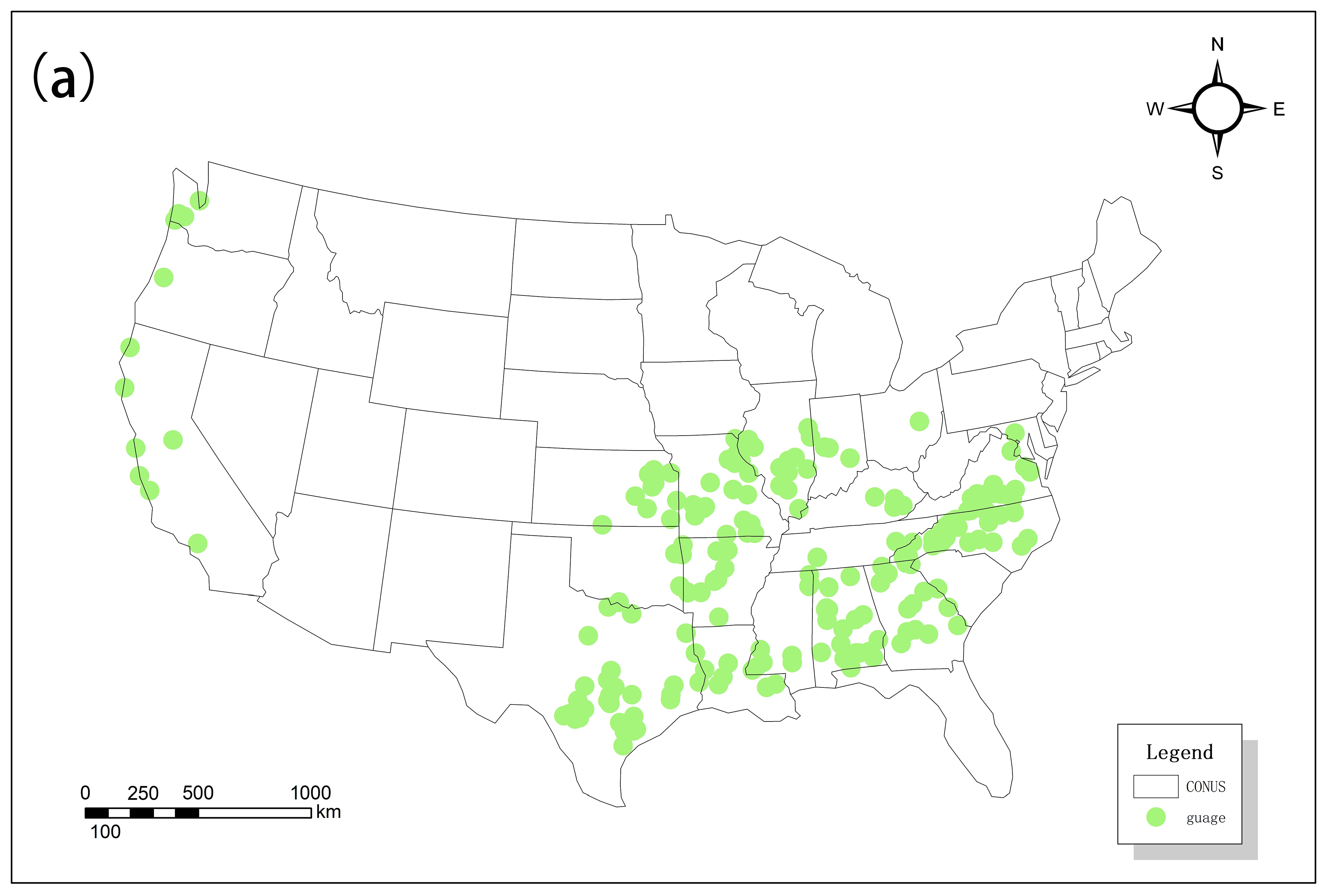
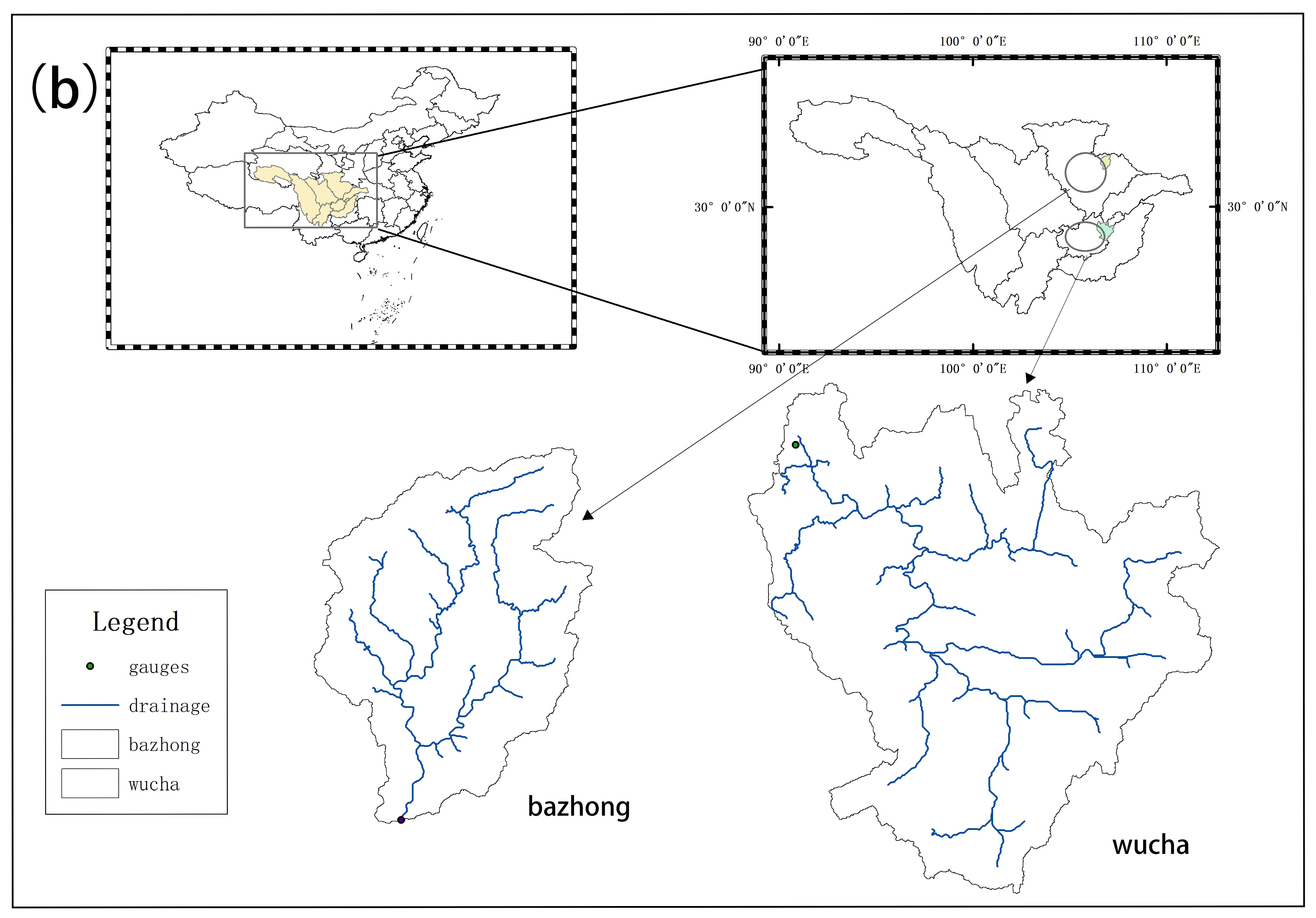
2.1. Study Area and Data

For this study, we used catchments from the Catchment Attributes and MEteorology for Large-sample Studies (CAMELS) data set [52], which covers 671 catchments in the contiguous United States (CONUS) that are minimally impacted by human activities, which is suitable for model calibration. In the CAMELS data set, hydrometeorological forcings were derived rom DAYMET and streamflow time series were retrieved from USGS observations.
The CAMELS data set also includes catchment-averaged land cover, soil and geology data; however, some data used to generate the CAMELS data set are not globally available (e.g., elevation and soil data). To ensure that the data of the US and Chinese catchments were consistent, we used various remote sensing data to generate the underlying surface data needed to drive the model.
We used the 30 m Global Digital Elevation Model (GDEM) from the Advanced Spaceborne Thermal Emission and Reflection Radiometer (ASTER) satellite to derive the surface elevation distribution in the catchment, which provides the basis for estimating other terrain-related variables. The land cover data we chose were from the 0.5 km MODIS-based Global Land Cover Climatology developed by Broxton et al. [53] based on the MODIS land cover (MCD12Q1, Collection 5.1) product. We also used the High-Resolution Global Map of Soil Hydraulic Properties [54] to obtain the soil-related characteristics.
The XAJ model is a rainfall-runoff model that is applicable only in humid and semihumid regions dominated by the saturation excess runoff yield mechanism. Therefore, for this study, we selected only catchments in which the annual precipitation was greater than 800 mm, there were fewer than 30 days of snow cover and the wet land area was less than 10%. A total of 196 catchments located primarily in the western and southeastern US met our criteria (Figure 1a). Details of these catchments can be found in the Supplementary Materials.
To better evaluate the parameters estimated by the ML approach, we also selected two catchments, Bazhong and Wucha, in the Jialing River Basin (one of the largest subbasins within the Yangtze River Basin), China, to perform cross-validation (Figure 1b). The drainage area of those two catchments are 2737 km2 and 5566 km2, respectively. The precipitation was derived from China’s meteorological forcing dataset which combines the TRMM satellite precipitation estimates and ground observations. Other hydrological data, including discharge and pan evaporation data, were collected and processed by the Hydrological Bureau of the Changjiang Water Resources Commission. We used three years of data (2013–2015) for validation purpose. The original data we collected had different temporal resolutions, so we linearly interpolated these hydrological data into a daily time step to drive the XAJ model.

2.2. XAJ Hydrological Model

The XAJ model was developed based on the saturation excess runoff yield mechanism, which dominates the runoff yield processes in humid and semihumid regions [6]. The XAJ model divides catchments into several subcatchments based on the corresponding terrain and vegetation conditions and then simulates the hydrological processes in each subcatchment in three stages: runoff yield, runoff separation and runoff routing. All subcatchments are linked by the main stream, and the outflow of each subcatchment is routed through the main stream by the Muskingum method. Readers are referred to Zhao [6] for more details on the XAJ model, including theory, structure and parameters. This paper mainly addresses the routing component of the XAJ model at the subcatchment scale. As discussed in the Introduction, due to the high heterogeneity of the stream network in a subcatchment, the XAJ model uses a conceptual component to represent the lumped attenuation and lag effects of the stream network on streamflow:
T Q ( t ) = C S × T Q ( t 1 ) + ( 1 C S ) × Q I N ( t L )
where TQ is the outflow of the subcatchment (L3/T), QIN is the XAJ-simulated inflow to the stream network of the subcatchment (L3/T) and CS (-) and L (T) are two parameters reflecting the attenuation and lag effects of the stream network, respectively.
According to the theory of hydrological processes, CS should be affected mainly by topographic indices such as the stream geometry, shape of the catchment, slope, etc. We relied on the ML technique to explore the relationships with these variables.

2.3. Baseline Model Calibration

To apply ML, we first calibrated the XAJ model for the 196 CAMELS catchments. We followed the same calibration strategy as reported in [55]. Before calibration, we calculated WM and SM using remote sensing data to reduce the potential nonuniqueness of the parameters. For the remaining parameters, we used a two-stage approach for calibration: we first introduced Model-Independent Parameter Estimation and Uncertainty Analysis (PEST) [56] to provide an optimized combination of parameters and then applied the conventional trial-and-error method to adjust some parameters based on our experience, to calibrate the XAJ model and ensure the consistent simulation of both high- and low-flow hydrographs.
Given that the data periods of the CAMELS catchments differ (see the Supplementary Materials), we used 70% of the data for calibration, while the remaining 30% were used for validation purposes. Both the calibration and the validation were conducted at a daily time scale. We examined both the relative error of the total runoff volume (bias, Equation (2)) and the Nash–Sutcliffe efficiency (NSE, Equation (3)) to determine the model performance in a specific catchment:
B i a s = V s i m V o b s V o b s × 100 % V s i m = i = 1 n 1 Q s i m , i + Q s i m , i + 1 2 Δ t i V o b s = i = 1 n 1 Q o b s , i + Q o b s , i + 1 2 Δ t i
N S E = 1 i = 1 n ( Q o b s , i Q s i m , i ) 2 i = 1 n ( Q o b s , i Q o b s ¯ ) 2
where Q o b s , i and Q s i m , i are the observed and modeled discharge (L3/T) at time step i, respectively, n is the total time step and Δti is the interval between time steps i and i + 1 (T).
We calibrated the model to have a bias of less than 5% to ensure the water balance of the simulation. We then set an NSE cutoff value of 0.5 for selecting catchments for further ML modeling.
Note that due to the nonuniqueness of the parameters, we assumed that the model parameters were constant over the catchment and calibrated only a single parameter value. Since most of the CAMELS catchments used herein were relatively small, we believed such an assumption was reasonable.

2.4. Estimating CS Using a Gradient-Boosted Regression Tree (GBRT)

Many ML algorithms have been used in the hydrology community. As reviewed by Zounemat-Kermani et al. [57], the boosting techniques have been more frequent and successfully implemented in hydrological problems than the bagging, stacking and dagging approaches. It is also documented that the gradient-boosted regression tree (GBRT) can outperform individual methods of classification and regression trees [58]. Our previous work further confirmed the potential capability of the GBRT in predicting model parameters. As such, we decided to adopt the GBRT to test our hypothesis.

2.4.1. Basic Theory of GBRT

The GBRT [59] is an ML method that combines basic regression trees and boosting to perform nonlinear regression and classification. The motivation of the GBRT is to add additional trees in sequence without changing the model parameters that have already been added to minimize a loss function of the training data. After learning, weak decision trees (i.e., weak prediction models) are combined into a powerful committee classifier [60]. The GBRT is also capable of evaluating the most important variables that affect targets. These features make the GBRT the preferable tool for determining the most significant underlying surface characteristics that affect CS and establishing a model for estimating CS.
The technical details of the GBRT can be found in [59]. We used the Scikit-learn (sklearn) module in Python to construct the GBRT model [61].
Several parameters of the GBRT should be optimized to achieve good performance, including the depth of the trees (max_depth, the maximum depth of the regression tree), number of weak learners (n_estimators, the maximum number of iterations of weak learners) and learning rate (learning_rate, the weight decay coefficient of each base learner). All these parameters are dimensionless.

2.4.2. Initial Selection of Independent Predictors

The selection of independent predictors is crucial for the GBRT, and appropriate predictors should meet the following criteria: (1) no significant correlation should exist among the predictors; (2) the predictors should have impacts on the target; and (3) the predictors should be estimated from the available data set.
After analyzing the routing process within each subcatchment, we selected seven underlying surface indices as predictors for the further application of the GBRT. Table 1 lists the predictors and their corresponding definitions. All these indices were derived at the subcatchment level where CS can be calibrated.

2.4.3. Construction of the GBRT Prediction Model

All indices in Table 1 were calculated for each catchment. We divided all the catchments into training (156 catchments) and testing (40 catchments) groups. The training groups were used by the GBRT to explore the relationships between the calibrated CS and various indices and to establish the prediction model. The prediction model was then used to estimate CS using the indices in the testing group, and the result was compared with the calibrated CS to validate the GBRT model.
Studies have reported that the selection of training samples may affect the generalization of ML [33]. To ensure the robustness of the prediction model, we used five different combinations of catchments for training, which were selected by assigning different random seeds. As such, we developed 5 different GBRT models (Models #1∼#5) to estimate CS in this study.
Based on the technical document of the GBRT [59] and previous studies (e.g., [62]), we defined the parameter range and step size for calibration (Table 2). We then applied the complete trial-and-error method (i.e., testing all possible combinations of parameters) to determine the best parameter.

2.5. Validation of the GBRT-Estimated CS

We evaluated the accuracy and robustness of the GBRT-estimated CS by performing the following steps.
We first compared the GBRT-estimated CS with the calibrated CS, directly enabling us to evaluate the performance of the GBRT and the accuracy of the GBRT-estimated CS.
We then ran the XAJ model using both the calibrated and the GBRT-estimated CS values and compared the metrics of the simulated streamflow, enabling us to evaluate the applicability of the GBRT-estimated CS in hydrological simulations.
The above evaluations were based on the CAMELS catchments. Finally, we used the best GBRT model to estimate the CS in the two catchments within the Jialing River Basin and evaluated the metrics of the simulated streamflow. This allowed us to evaluate the robustness of the GBRT-estimated CS.

3. Results

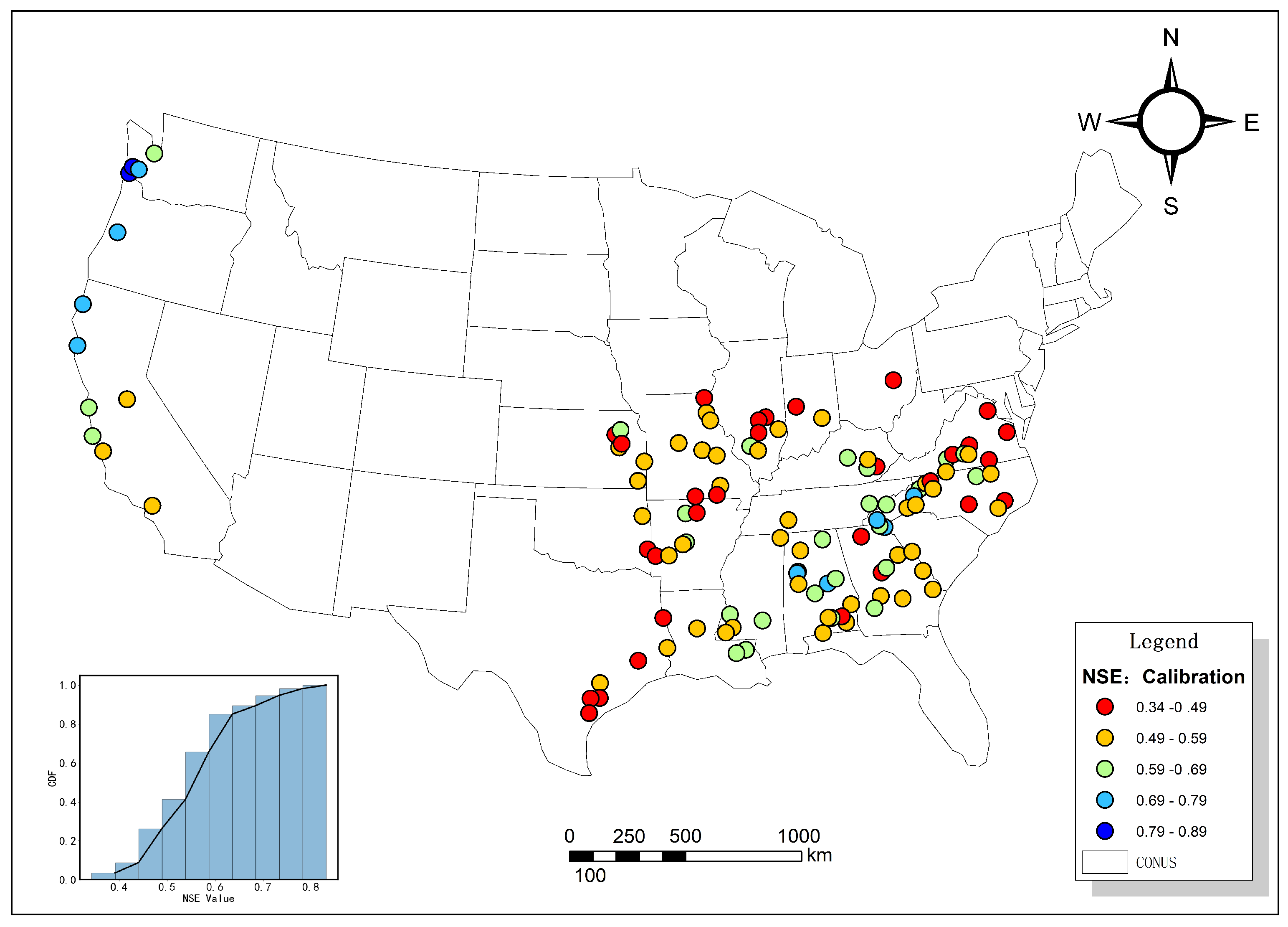
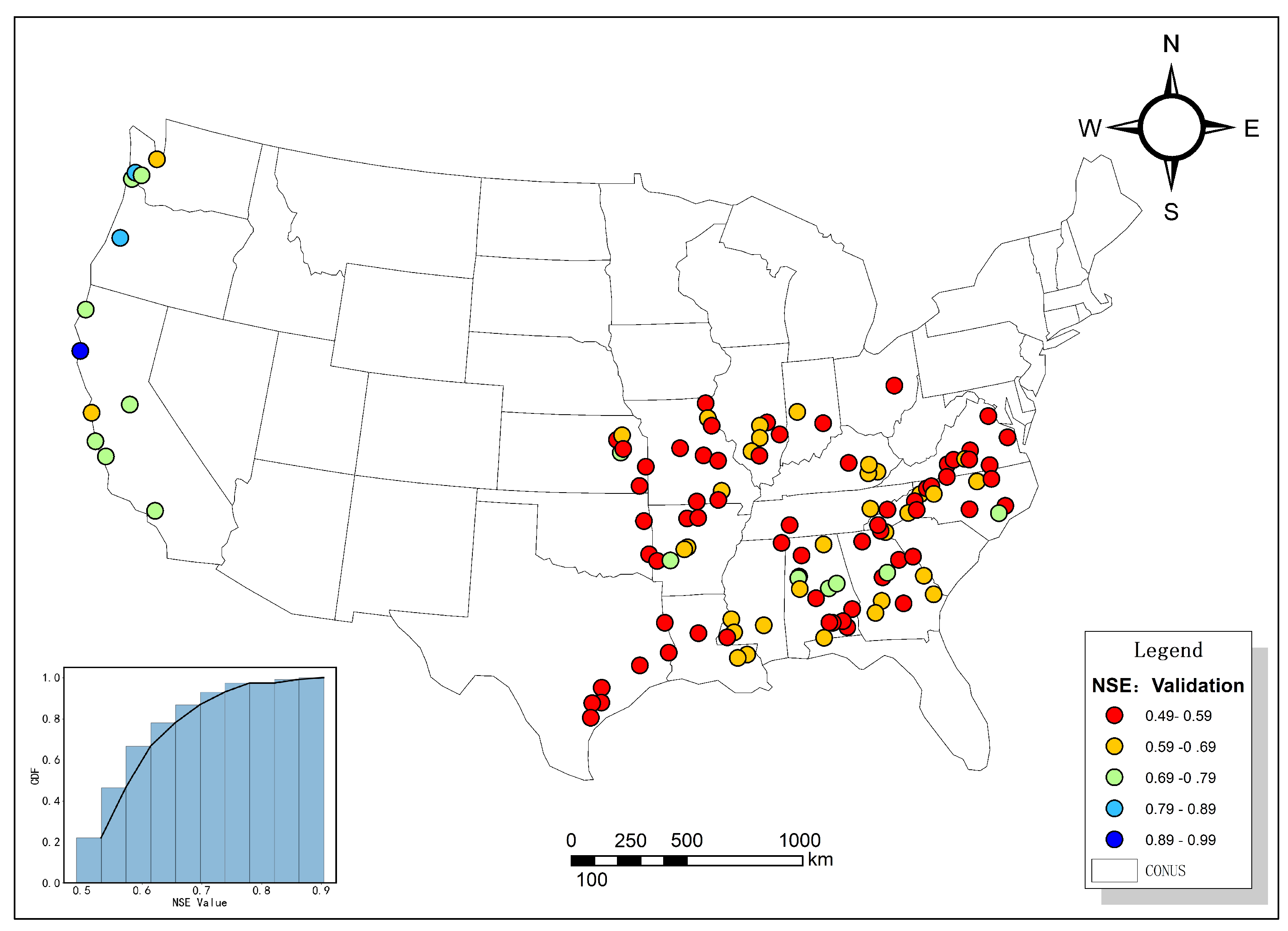
3.1. Calibration of the XAJ Model in the CAMELS Catchments

Following the above calibration strategy, we performed a two-stage calibration for all 196 catchments in the CAMELS data set suitable for the XAJ model. The calibrated CS values ranged from 0.10 to 0.87, which was a reasonable range. Figure 2 and Figure 3 show the NSE values averaged over the calibration and validation periods, respectively. According to the results, 117 (60%) catchments had an NSE ≥ 0.5 for the calibration period, and 114 (58%) catchments had an NSE ≥ 0.5 for the validation period. All catchments had a bias ≤5%, which indicated an acceptable water balance. The model performance was consistent between the calibration and validation periods, and we did not find significant degradation of the model performance in the validation period.
As reported by [63], simulations using the coupled Snow17 snow model and the Sacramento Soil Moisture Accounting Model in 671 CAMELS catchments showed that, at the monthly scale, 90% of the catchments displayed an NSE ≥ 0.55 for the calibration period, and 34% exhibited an NSE ≥ 0.8. Since it is more difficult to obtain a higher NSE at a finer temporal scale (i.e., the daily scale in this study), we assumed that the 114 catchments with an NSE ≥ 0.5 had a sufficient model skill; therefore, the calibrated parameters, including CS, were considered reasonable and were used for further analysis.

3.2. Importance of the Selected Predictors

After optimizing the parameters of the GBRT (Table 3), we used the results from five GBRT models to investigate the importance of the selected predictors. Figure 4 shows the importance index of seven predictors evaluated by the GBRT models. In this figure, the importance index is expressed by a color ramp, with yellow representing the largest value. To make it clearer, Figure 4 also shows the ranking of different predictors with one corresponding to the most important predictor and seven corresponding to the least important predictor. According to Figure 4, regardless of the combination of training catchments, the GBRT identified the drainage density (Dd), stream source density (Dss) and area (A) as the most important factors. All models except model #1 identified the drainage density (Dd) as the most important factor, with the importance index ranging from 0.22 to 0.38. The other four predictors exhibited relatively low important levels. The shape factor was the least important predictor, with the importance index ranging from 0.04 to 0.1. We used the five most significant variables to construct the GBRT model.

3.3. CS Estimation and Hydrological Simulation

Prediction models were developed using the training catchments. Because we used five different catchment combinations for training purposes, we developed five different prediction models (Models #1–#5) to derive CS. The solid lines in Figure 5 denote the metrics of the different models in predicting CS from the training catchments. The performances are consistent among the different prediction models, confirming the robustness of the GBRT for estimating CS. Model #1 has a relatively better performance, with r, RMSE and MAE values of 0.96, 0.06 and 0.04, respectively. The other models yield comparable results.
Next, CS was derived for the testing catchments using the same models developed from the training catchments, and the dashed lines in Figure 5 denote the corresponding metrics. The performances of the testing catchments are worse than those of the training catchments. Model #1 has a relatively good performance, with r, RMSE and MAE values of 0.74, 0.11 and 0.10, respectively. In contrast, Model #3 has the worst performance in terms of r (0.73, Figure 5a), while Model #2 has the worst performance in terms of the RMSE and MAE (0.13 and 0.11, respectively, Figure 5b,c). Figure 6 shows a scatter plot between the calibrated and GBRT-derived CS values in the testing catchments, showing that most points are distributed along the 1:1 line regardless of the models. The correlation coefficient (r) ranges from 0.73 (Model #3) to 0.80 (Model #4 and #5). Hence, these evaluations confirm that the GBRT models have relatively good performance when estimating CS.
To evaluate whether the GBRT-estimated CS could be used in hydrological simulations, we used the XAJ model to carry out simulations using data from 23 catchments in the testing group. Figure 7 presents a box plot of the NSE of the runoff simulations using the GBRT-estimated and calibrated CS values. The boxes in this figure represent the distribution of CS values among these 23 catchments. Our results showed that, due to the bias of CS, the NSE of several catchments using the GBRT-estimated CS was less than 0.5—the cutoff value we defined. The lowest NSE was only 0.23 from GBRT Model #5. Although the NSE degraded in several catchments, we compared the shapes of the boxes and found that the NSE values of the simulations were comparable even when using different values of CS, especially for the catchments with an NSE above the first quartile (25%). Among all five GBRT models, Model #2 had the best performance; there were no significant changes in the NSE, and the r of the NSE from Model #2 was 0.92 (figure not shown).
We also examined the relationship between ΔCS (i.e., the GBRT-estimated CS minus the calibrated CS) and ΔNSE (i.e., the GBRT-estimated NSE minus the calibrated NSE) to better understand how the bias of CS could affect the streamflow simulations. As shown in Figure 8, there was no clear pattern between ΔCS and ΔNSE due to the nonlinearity of the hydrological model; however, most catchments (93.5%) exhibited a ΔNSE within the ±0.1 limit (solid line in Figure 8). Two catchments (both in Model #5) experienced a decrease in NSE exceeding 0.2; the largest reduction in the NSE was −0.34 in Model #5, and the corresponding ΔCS was 0.22.
Based on Figure 7 and Figure 8, we found that, although a bias existed between the GBRT-estimated and calibrated CS, simulations using the GBRT-estimated CS could still achieve results that were comparable to those using the calibrated CS. Most catchments had a ΔNSE within the ±0.1 limit. Thus, the overall robustness and accuracy of the simulated runoff using the GBRT-estimated CS could be guaranteed.
Among all five models, Model #2 had a relatively good performance. Therefore, we utilized Model #2 to estimate the CS in two catchments, namely, Bazhong and Wucha, within the Jialing River Basin and evaluate the results. Using the GBRT estimation model, we could assign different CS values to different subcatchments depending on their unique morphometric characteristics. Figure 9 shows the resulting spatial distribution of CS over the Bazhong and Wucha catchments. Figure 10 shows three series of runoff: (1) observed runoff, (2) simulated runoff using the GBRT-estimated CS (spatially distributed) and (3) simulated runoff using the calibrated CS (spatially lumped). Only the results from the validation period are plotted. As shown in Figure 10, the simulations with the GBRT-estimated CS yielded NSE values of 0.37 and 0.65 for the Wucha and Bazhong catchments, respectively, and have corresponding bias values of −5.98% and 7.4%. Although a degradation of the NSE and bias could be observed, the simulations using the GBRT-estimated CS still captured the streamflow series well, and the results were comparable to those using the calibrated CS.

4. Discussion

4.1. Factors Affecting the Routing Process

In the hydrology community, flood routing in a main stream is described by either the Saint-Venant equations or by the Muskingum method. However, at the scale of the computational units of hydrological models (∼102 to ∼103 m2), it is difficult and often unnecessary to simulate the flood routes in each of the relatively small tributaries. As such, many hydrological models, especially conceptual models, treat the entire stream network in a computational unit as a system, simulate the lumped routing processes and obtain the outflow at the subcatchment outlet (e.g., [6,64,65]).
In the XAJ model, CS reflects the lumped attenuation effects of the stream network in the subcatchment on streamflow. Our results indicate that the drainage density (Dd), the stream source density (Dss) and the area of the catchment (A) are the three major factors that have the most significant impact on CS. Our findings are supported by previous studies focusing on routing processes.
The drainage density has long been recognized as an important factor that regulates hydrological responses [66,67,68,69] and thus has been used to predict various hydrological variables, including the Soil Conservation Service (SCS) curve number [29], erosion rate [70] and base flow index [71], among many others. For the routing problem considered in this study, if all other factors remain the same, the travel time of streamflow in a stream decreases with increasing drainage density (Dd), which leads to weaker attenuation effects, as reflected by CS. Moreover, high values of Dd are usually related to impervious hill slopes and steeper slopes [67], which also have indirect impacts on the flow regime in tributaries. Our results are in accordance with those of previous studies carried out on both natural hill slopes [72] and real catchments [73].
Compared with the drainage density (Dd), the stream source density Dss is less commonly used to quantify hydrological processes. As reported by [74], the influence of a deviation in the channel storage volume is significant in mountain rivers. In our study, catchments with a higher Dss indicate more small tributaries with small storage volumes, which have relatively weaker attenuation effects compared with higher-order streams. The area (A) also has a significant control on the routing, and a small catchment tends to be dominated by hill slope processes [73]; therefore, the attenuation effects of the stream are weak, leading to a small CS.

4.2. Implications of This Study

Our results (Figure 5 and Figure 6) proves the GBRT ML approach can effectively capture the nonlinear relationships between CS and various environmental effects. After the evaluation using the XAJ model, although differences were noted between the GBRT-derived and calibrated CS, the resulting bias in the simulated runoff was still in an acceptable range (Figure 7 and Figure 8). Validations in two catchments of the Jialing River Basin further confirmed the applicability of the GBRT-derived parameter. All these findings confirmed our initial hypothesis.
Previous studies regarding the estimation of CS mainly relied on conventional regression or even linear regression approaches, and these studies identified catchment area and slope as dominant factors affecting CS [22,46]. Our results showed that the drainage density, stream source density and catchment area were three dominant factors while the slope was less important. To better understand the difference, we carried out a linear regression to investigate the correlation between CS and seven predictors as defined in Table 1. From Figure 11, we can clearly see that their exist certain relationships between catchment area (Figure 11a), drainage density (Figure 11d), stream source density (Figure 11e) and CS. However, such relationships cannot be simply retrieved by a linear regression since the linear correlation coefficient (r) is small. In contrast, the GBRT models we developed are able to capture such complex relationships. In terms of the slope, the linear correlation between CS and the slope is weak with r being 0.02 and the significance level (p) being 0.82 (Figure 11b). One possible reason is that CS is determined by the slope of the stream network rather than the average slope of the catchment. However, it is impossible to determine the slope of the stream network due to the DEM accuracy in a water body [75]. Figure 11b further proves that when estimating CS using several catchments based on a linear regression, the results might be unreliable and difficult to extrapolate to other catchments.
Our study also demonstrates the benefits of quantitatively estimating CS. One obvious benefit of the GBRT approach is that the XAJ model can be applied to ungauged catchments for which streamflow observations are unavailable or impaired catchments in which the natural streamflow is affected by human activities. Benefiting from the Earth Observing System (EOS), many hydrological variables related to runoff yield, such as sediment transport, soil moisture and land surface temperature, can be accurately retrieved from remote sensing data. Many studies have confirmed the applicability of remote sensing data for calibrating parameters related to runoff yield processes [55,76,77]. This is especially helpful for models focusing on runoff yield processes (e.g., global land models). In contrast, although some encouraging results in estimating the river discharge or stage from satellite data have been reported [78,79], the use of satellite data to constrain the calibration of runoff routing parameters remains challenging. As such, the regionalization of runoff routing-related parameters should be studied with some urgency, and our work provides a framework that can be extended to other models. Moreover, by using the GBRT approach, the spatial distribution of CS can be derived for a large catchment (Figure 9), which can better reflect the spatial heterogeneity of the catchment. Although many hydrological models have been designed to represent the spatial heterogeneity of the land surface, the traditional calibration method on a limited number of discharge stations lumps all hydrological processes together [77], which makes it difficult to reflect the real spatial pattern of parameters. Our approach therefore offers an alternative to estimate spatially distributed parameters that better satisfy the requirements of distributed models.

4.3. Limitations and Future Directions

To make the results more reliable and robust, we selected 196 catchments and developed five models to explore the relationship among CS and various predictors. However, several limitations still exist which can be addressed in future studies. First of all, due to data availability, we mainly focused on catchments with an average slope less than 16°. Studies have documented that runoff processes in steep slopes or catchments are quite different from those with moderate slope [80,81]. Considering catastrophic flash floods often occur in steep catchments, it is therefore necessary to study the parameters estimation approach in order to better predict the occurrence of flash floods using hydrological models. Moreover, we only used one specific ML model, the GBRT, in this study. Although previous studies and our results have demonstrated the capabilities of the GBRT, other models such as an ANN and 1D-CNN may also get comparable performances. It is therefore necessary to carry out a more detailed study to evaluate different models. Last but not least, in this study, we focused only on one specific parameter of the XAJ model, i.e., CS. However, our scheme can be easily extended to other model parameters or other hydrological models to improve the performance of models.

5. Conclusions

In this paper, we combined remote sensing data and a machine learning (ML) scheme, namely, the gradient-boosted regression tree (GBRT), to establish models to quantitatively estimate the routing parameter CS in the XAJ model. We chose 114 catchments from the Catchment Attributes and MEteorology for Large-sample Studies (CAMELS) data set suitable for the XAJ model and performed good runoff simulations after calibration. We used the GBRT to explore the relationships between the calibrated CS and various underlying surface characteristics in the 114 catchments, based on which we established five prediction models based on different catchment combinations. The following conclusions can be drawn from this study:
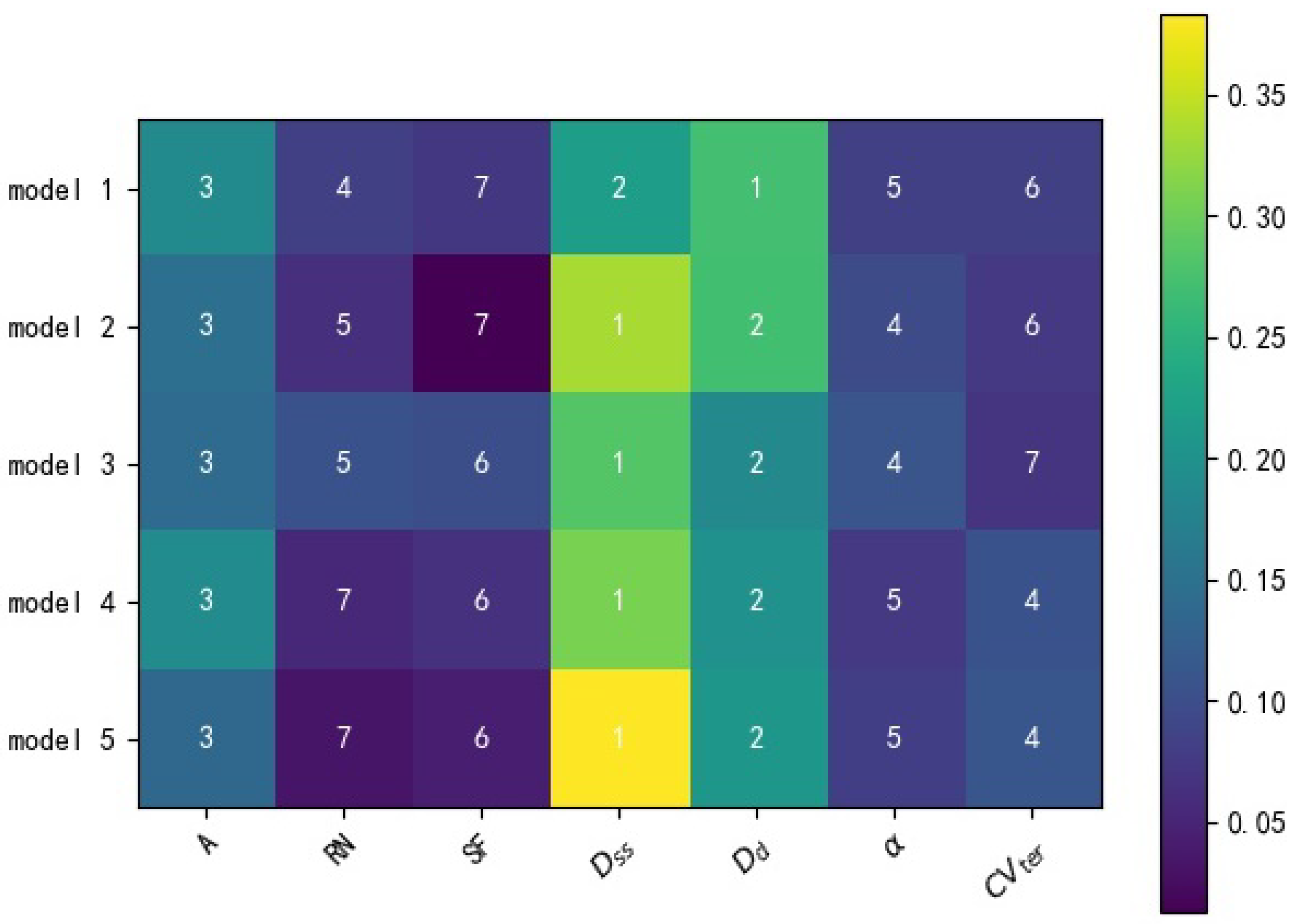
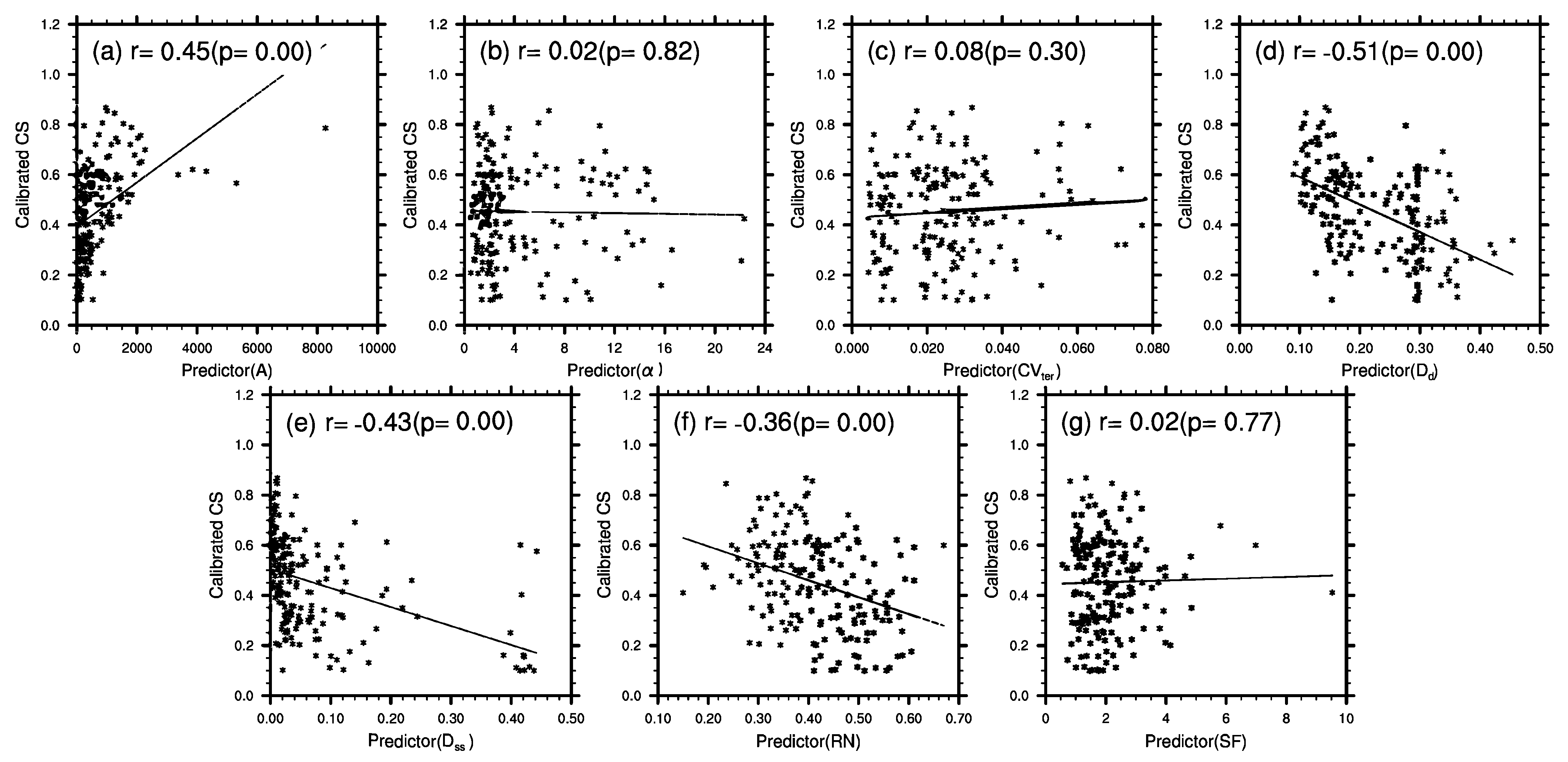
  • The drainage density, stream source density and area of the catchment are the three major factors with the most significant impact on CS. This outcome is reasonable based on an examination of the physical discipline of runoff routing.
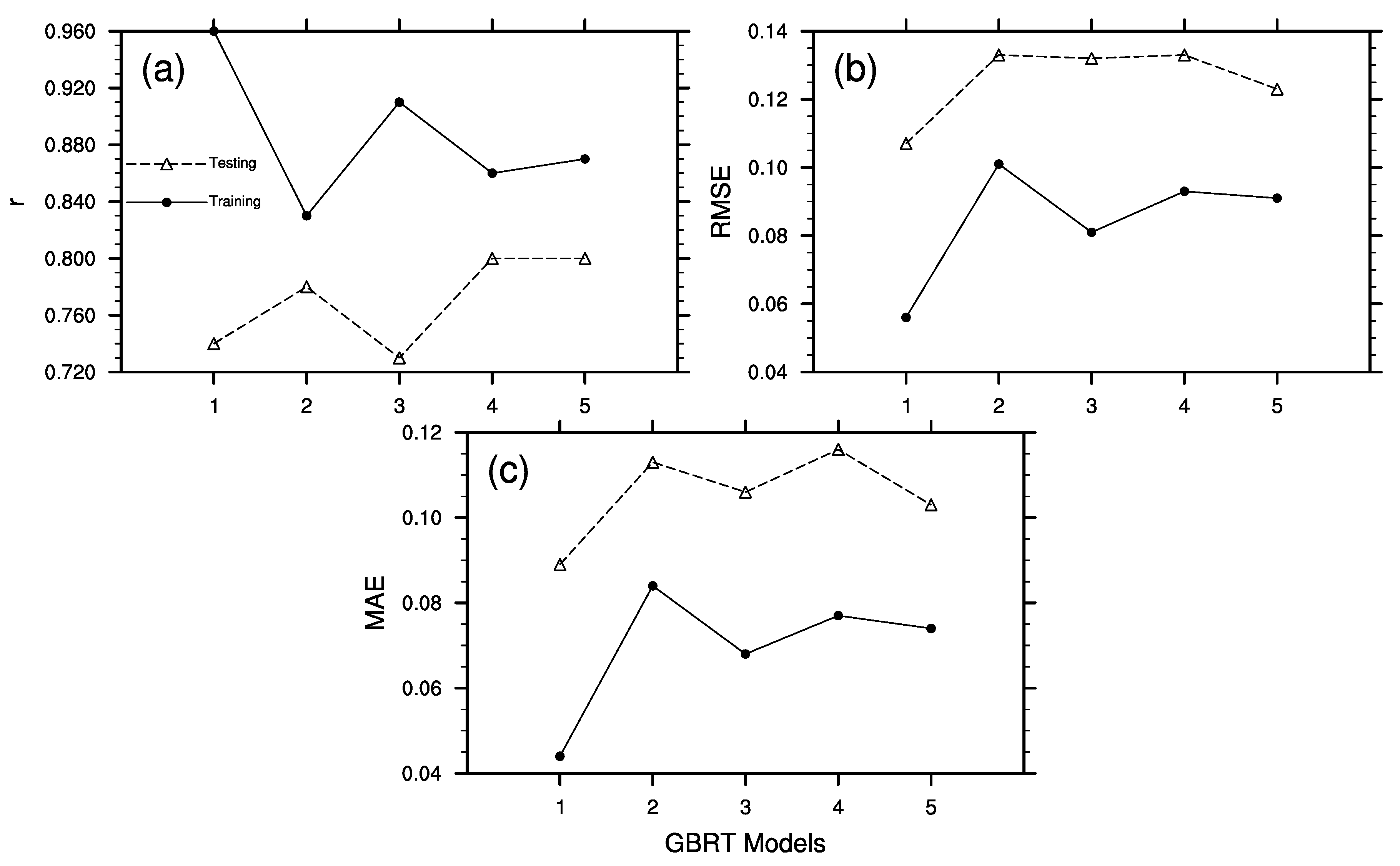
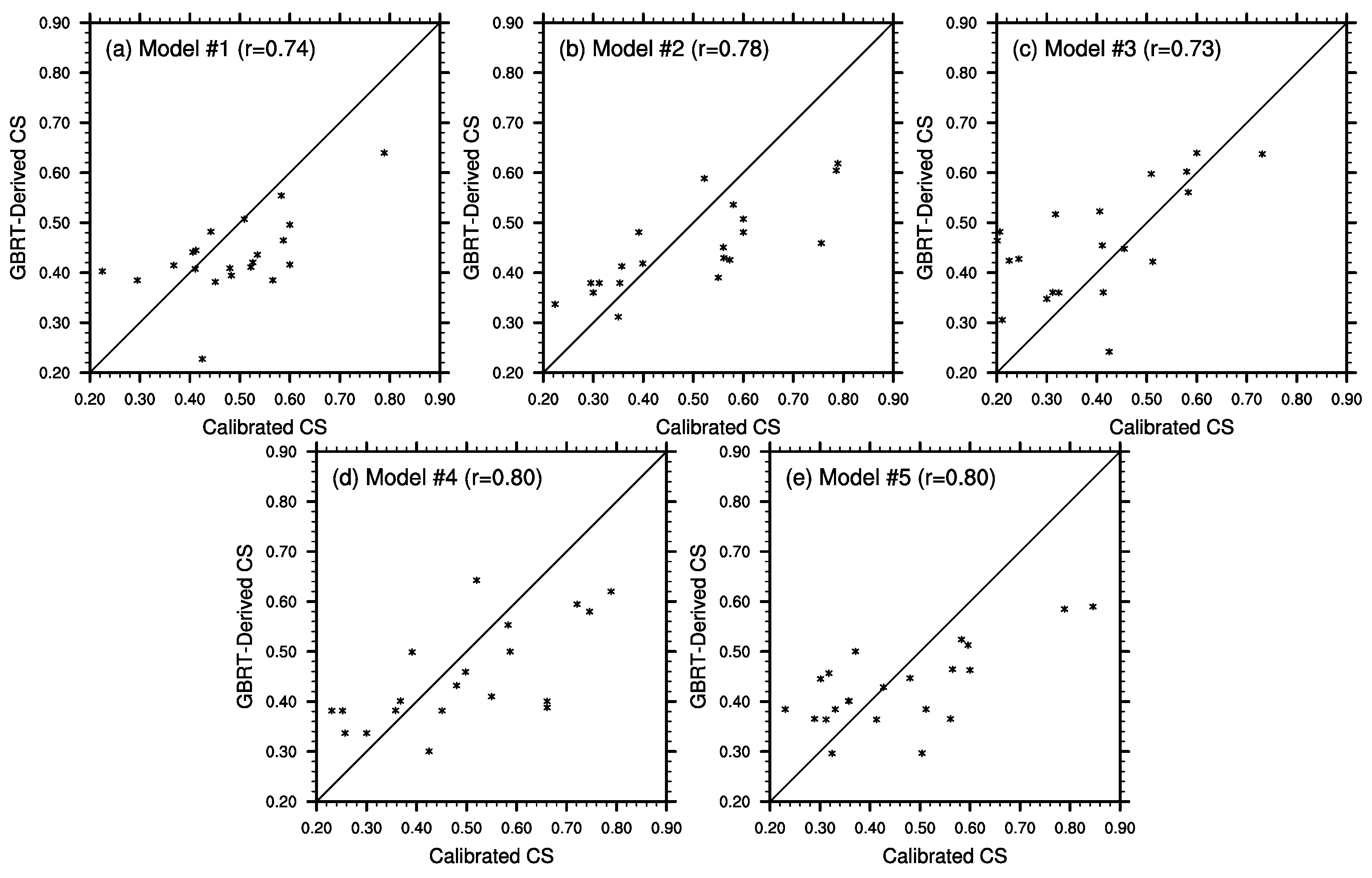
  • Overall, the CS values yielded by the prediction models we developed are comparable to those from the calibration. Considering the values of CS, the best model (Model #1) has a correlation coefficient (r), a root-mean-square error (RMSE) and a mean absolute error (MAE) of 0.96, 0.06 and 0.04, respectively, confirming the good performance of the GBRT for estimating CS.
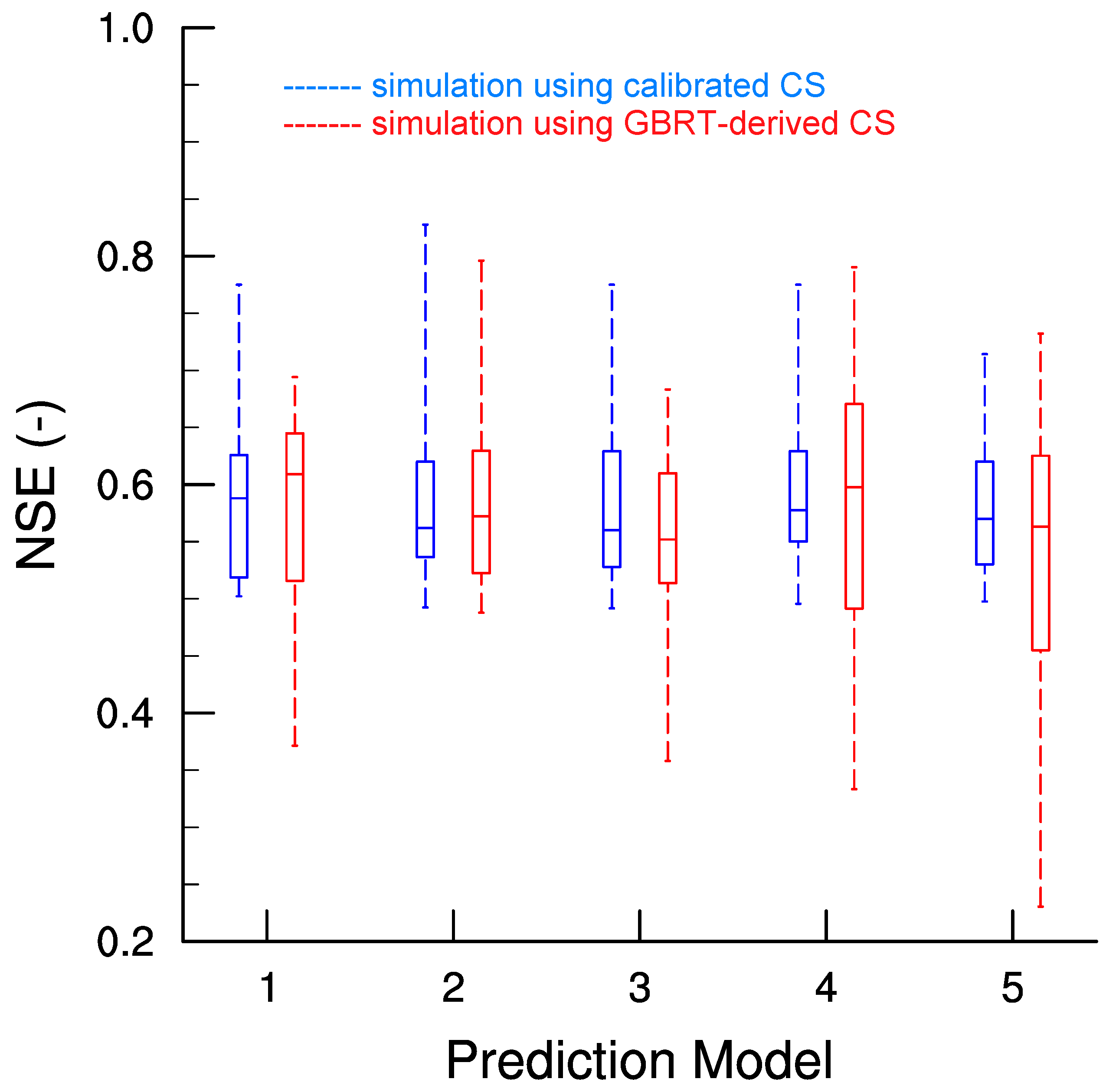
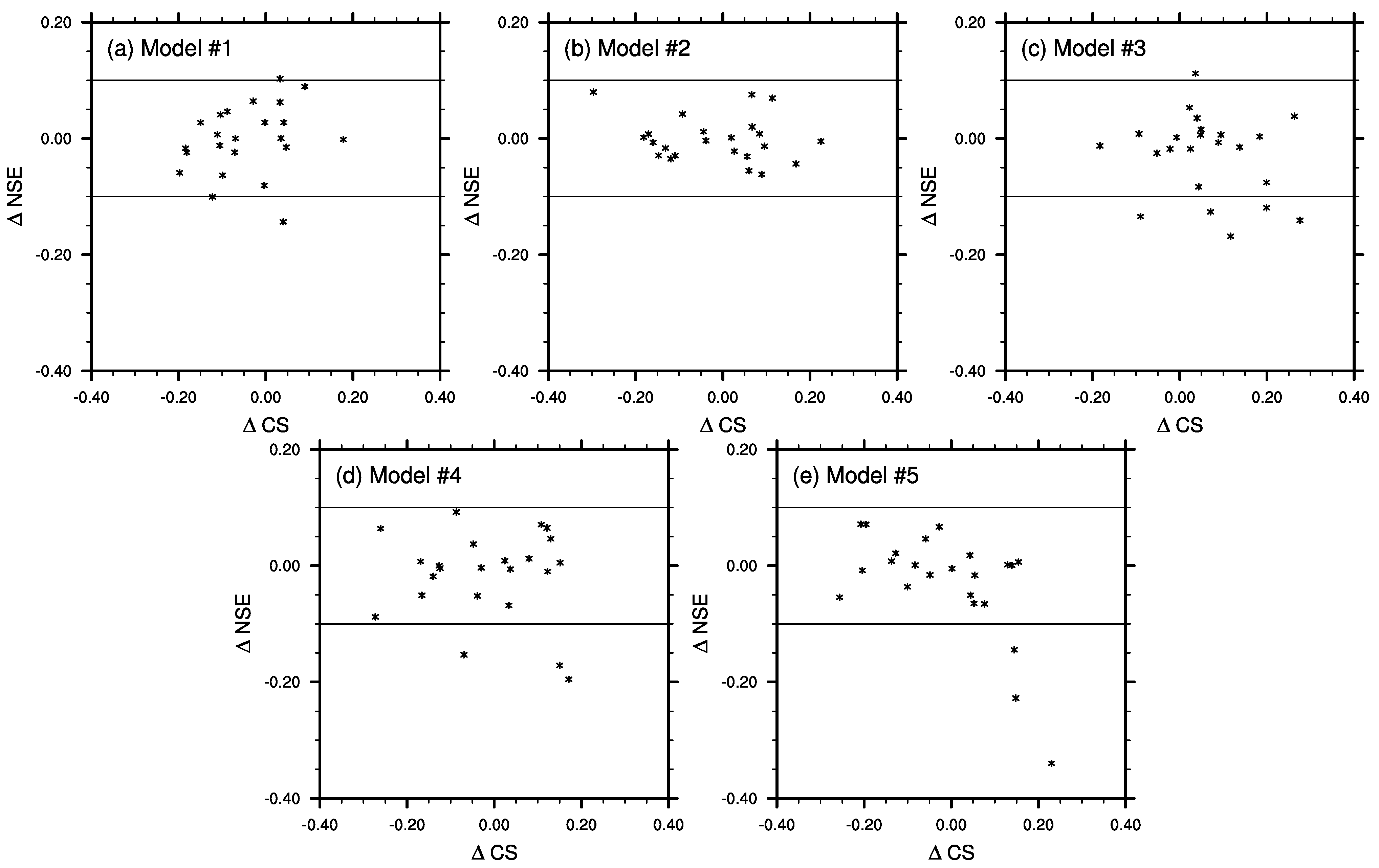
  • Although a bias exists between the GBRT-estimated and calibrated CS, runoff simulations using the GBRT-estimated CS can still achieve results comparable to those using the calibrated CS. Most catchments have a ΔNSE within the ±0.1 limit.
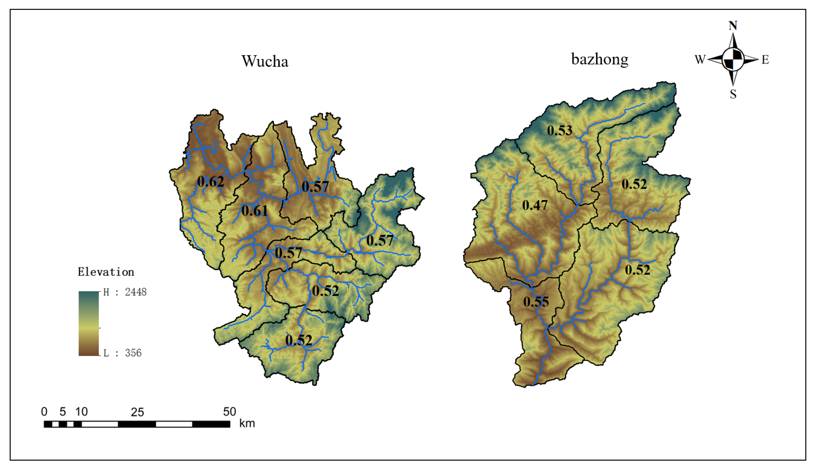
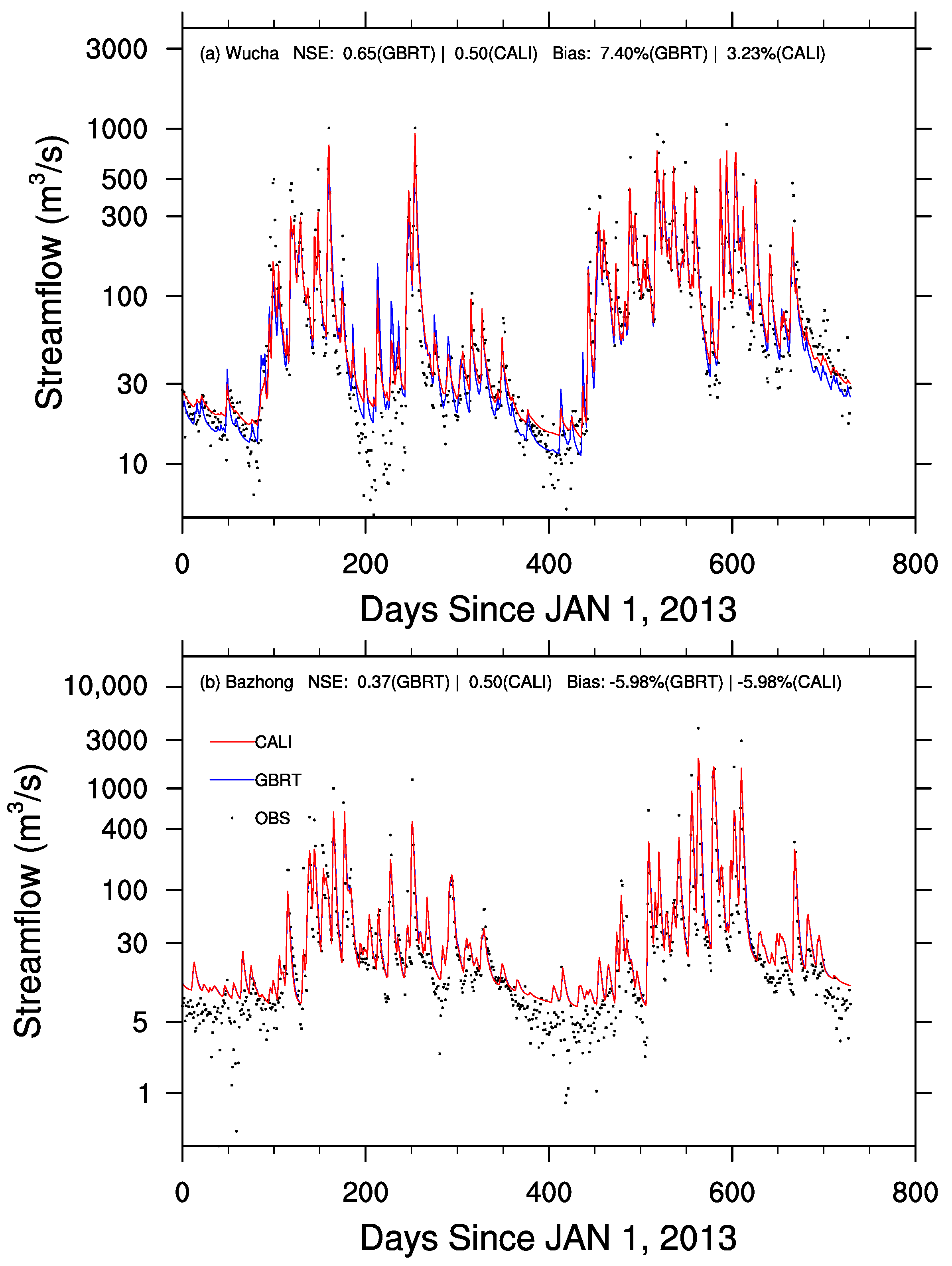
  • Validations in two catchments further verify that the GBRT-estimated CS can be used for hydrological simulations and can reflect the spatial patterns of parameters and therefore better exploit the benefits of distributed models.
This paper confirmed the hypothesis that: (1) with the help of a large sample of catchments and associated remote sensing data, an ML-based approach can capture the nonstationary and nonlinear relationships between CS and underlying surface characteristics; and (2) CS estimated by ML from large samples has a robustness that can guarantee the overall performance of the XAJ mode. Comparing with previous studies, this paper proposed a more reliable and robust ML-based model to estimate CS, which advanced the methodology for quantitatively estimating the parameters of hydrological models. Our approach offers an alternative to estimate spatially distributed parameters that better satisfy the requirements of distributed models.
Several limitations still exist including the routing process on steep slopes, the performance of other ML algorithms and the estimation of other parameters. These limitations can be addressed by further studies.

Supplementary Materials

The following supporting information can be downloaded at: https://www.mdpi.com/article/10.3390/rs14184609/s1, Details of CAMELS catchments used for this study.

Author Contributions

Conceptualization, Y.F. and X.Z.; methodology, Y.F., Y.H. and T.Z.; validation, B.Q.; analysis, Y.F. and D.X.; writing, all authors. All authors have read and agreed to the published version of the manuscript.

Funding

This study was funded by the Natural Science Foundation of China (U2240216, 51809074), Henan Province Science Foundation for Youths (212300410202), and National Key R&D Program of China (2019YFC0409000).

Data Availability Statement

The CAMELS data set can be downloaded through https://dx.doi.org/10.5065/D6MW2F4D (accessed on 4 January 2021). The High-Resolution Global Map of Soil Hydraulic Properties can be downloaded through https://dx.doi.org/10.7910/DVN/UI5LCE (accessed on 4 January 2021). The hydrological data of the two Chinese catchments can be obtained by contacting the corresponding author.

Acknowledgments

We would like to thank assistant editors, academic editors and reviewers for their efforts to improve the quality of this paper. We also thank students Pingshan Qin and Zhongye Xia for polishing the figures.

Conflicts of Interest

The authors declare no conflict of interest.

References

  1. Paniconi, C.; Putti, M. Physically based modeling in catchment hydrology at 50: Survey and outlook. Water Resour. Res. 2015, 51, 7090–7129. [Google Scholar] [CrossRef]
  2. Fatichi, S.; Vivoni, E.R.; Ogden, F.L.; Ivanov, V.Y.; Mirus, B.; Gochis, D.; Downer, C.W.; Camporese, M.; Davison, J.H.; Ebel, B.; et al. An overview of current applications, challenges, and future trends in distributed process-based models in hydrology. J. Hydrol. 2016, 537, 45–60. [Google Scholar] [CrossRef]
  3. Niu, G.Y.; Paniconi, C.; Troch, P.A.; Scott, R.L.; Durcik, M.; Zeng, X.; Huxman, T.; Goodrich, D.C. An integrated modelling framework of catchment-scale ecohydrological processes: 1. Model description and tests over an energy-limited watershed. Ecohydrology 2014, 7, 427–439. [Google Scholar] [CrossRef]
  4. Freeze, R.; Harlan, R. Blueprint for a physically-based, digitally-simulated hydrologic response model. J. Hydrol. 1969, 9, 237–258. [Google Scholar] [CrossRef]
  5. Nijzink, R.C.; Almeida, S.; Pechlivanidis, I.G.; Capell, R.; Gustafssons, D.; Arheimer, B.; Parajka, J.; Freer, J.; Han, D.; Wagener, T.; et al. Constraining Conceptual Hydrological Models with Multiple Information Sources. Water Resour. Res. 2018, 54, 8332–8362. [Google Scholar] [CrossRef]
  6. Zhao, R.J. The Xinanjiang model applied in China. J. Hydrol. 1992, 135, 371–381. [Google Scholar] [CrossRef]
  7. Cheng, C.T.; Zhao, M.Y.; Chau, K.; Wu, X.Y. Using genetic algorithm and TOPSIS for Xinanjiang model calibration with a single procedure. J. Hydrol. 2006, 316, 129–140. [Google Scholar] [CrossRef]
  8. Hapuarachchi, H.A.P.; Li, Z.; Wang, S. Application of SCE-UA method for calibrating the Xinanjiang watershed model. J. Lake Sci. 2001, 13, 304–314. [Google Scholar]
  9. Kan, G.; He, X.; Ding, L.; Li, J.; Hong, Y.; Zuo, D.; Ren, M.; Lei, T.; Liang, K. Fast hydrological model calibration based on the heterogeneous parallel computing accelerated shuffled complex evolution method. Eng. Optim. 2018, 50, 106–119. [Google Scholar] [CrossRef]
  10. Li, Z.; Xin, P.; Tang, J. Study of the Xinanjiang model parameter calibration. J. Hydrol. Eng. 2013, 18, 1513–1521. [Google Scholar]
  11. Wu, Q.; Liu, S.; Cai, Y.; Li, X.; Jiang, Y. Improvement of hydrological model calibration by selecting multiple parameter ranges. Hydrol. Earth Syst. Sci. 2017, 21, 393–407. [Google Scholar] [CrossRef]
  12. Emanuel, R.E.; Hazen, A.G.; McGlynn, B.L.; Jencso, K.G. Vegetation and topographic influences on the connectivity of shallow groundwater between hillslopes and streams. Ecohydrology 2014, 7, 887–895. [Google Scholar] [CrossRef]
  13. Niu, G.Y.; Pasetto, D.; Scudeler, C.; Paniconi, C.; Putti, M.; Troch, P.A.; Delong, S.B.; Dontsova, K.; Pangle, L.; Breshears, D.D.; et al. Incipient subsurface heterogeneity and its effect on overland flow generation—Insight from a modeling study of the first experiment at the Biosphere 2 Landscape Evolution Observatory. Hydrol. Earth Syst. Sci. 2014, 18, 1873–1883. [Google Scholar] [CrossRef]
  14. Bárdossy, A.; Singh, S.K. Robust estimation of hydrological model parameters. Hydrol. Earth Syst. Sci. Discuss. 2008, 5, 1641–1675. [Google Scholar] [CrossRef]
  15. Yao, C.; Li, Z.; Yu, Z.; Zhang, K. A priori parameter estimates for a distributed, grid-based Xinanjiang model using geographically based information. J. Hydrol. 2012, 468–469, 47–62. [Google Scholar] [CrossRef]
  16. Gong, J.; Yao, C.; Li, Z.; Chen, Y.; Huang, Y.; Tong, B. Improving the Flood Forecasting Capability of the Xinanjiang Model for Small- and Medium-Sized Ungauged Catchments in South China; Number 0123456789; Springer: Dordrecht, The Netherlands, 2021. [Google Scholar] [CrossRef]
  17. Guo, Y.; Zhang, Y.; Zhang, L.; Wang, Z. Regionalization of hydrological modeling for predicting streamflow in ungauged catchments: A comprehensive review. WIREs Water 2021, 8, e1487. [Google Scholar] [CrossRef]
  18. Bao, Z.; Zhang, J.; Liu, J.; Fu, G.; Wang, G.; He, R.; Yan, X.; Jin, J.; Liu, H. Comparison of regionalization approaches based on regression and similarity for predictions in ungauged catchments under multiple hydro-climatic conditions. J. Hydrol. 2012, 466–467, 37–46. [Google Scholar] [CrossRef]
  19. Parajka, J.; Merz, R.; Blöschl, G. A comparison of regionalisation methods for catchment model parameters. Hydrol. Earth Syst. Sci. 2005, 9, 157–171. [Google Scholar] [CrossRef]
  20. Pagliero, L.; Bouraoui, F.; Diels, J.; Willems, P.; McIntyre, N. Investigating regionalization techniques for large-scale hydrological modelling. J. Hydrol. 2019, 570, 220–235. [Google Scholar] [CrossRef]
  21. Bao, W.; Li, Q. Estimating Selected Parameters for the XAJ Model under Multicollinearity among Watershed Characteristics. J. Hydrol. Eng. 2012, 17, 118–128. [Google Scholar] [CrossRef]
  22. Lu, M. New approach to synthesization of recession coefficients in Xinanjiang model. J. Hydroelectr. Eng. 2016, 35, 1–6, (In Chinese with English Abstract). [Google Scholar]
  23. Zang, S.; Li, Z.; Yao, C.; Zhang, K.; Sun, M.; Kong, X. A New Runoff Routing Scheme for Xin’anjiang Model and Its Routing Parameters Estimation Based on Geographical Information. Water 2020, 12, 3429. [Google Scholar] [CrossRef]
  24. Guo, W.J.; Wang, C.H.; Ma, T.F.; Zeng, X.M.; Yang, H. A distributed Grid-Xinanjiang model with integration of subgrid variability of soil storage capacity. Water Sci. Eng. 2016, 9, 97–105. [Google Scholar] [CrossRef]
  25. Shi, P.; Rui, X.F.; Qu, S.M.; Chen, X. Calculating storage capacity with topographic index. Adv. Water Sci. 2008, 19, 264, (In Chinese with English Abstract). [Google Scholar]
  26. Cao, X.; Ni, G.; Qi, Y.; Liu, B. Does Subgrid Routing Information Matter for Urban Flood Forecasting? A Multiscenario Analysis at the Land Parcel Scale. J. Hydrometeorol. 2020, 21, 2083–2099. [Google Scholar] [CrossRef]
  27. Meng, S.; Xie, X.; Liang, S. Assimilation of soil moisture and streamflow observations to improve flood forecasting with considering runoff routing lags. J. Hydrol. 2017, 550, 568–579. [Google Scholar] [CrossRef]
  28. Zhang, X.N.; Fang, Y.H.; Qu, B.; Ma, L.J.; Wu, M. Study on Parameters Estimation of the Xaj Model Based on Underlying Surface Characteristics. In Proceedings of the 37th IAHR World Congress, Kuala Lumpur, Malaysia, 13–18 August 2017. [Google Scholar]
  29. Heuvelmans, G.; Muys, B.; Feyen, J. Regionalisation of the parameters of a hydrological model: Comparison of linear regression models with artificial neural nets. J. Hydrol. 2006, 319, 245–265. [Google Scholar] [CrossRef]
  30. Schmidt, L.; Heße, F.; Attinger, S.; Kumar, R. Challenges in Applying Machine Learning Models for Hydrological Inference: A Case Study for Flooding Events Across Germany. Water Resour. Res. 2020, 56, e2019WR025924. [Google Scholar] [CrossRef]
  31. Mosavi, A.; Ozturk, P.; Chau, K.W. Flood prediction using machine learning models: Literature review. Water 2018, 10, 1536. [Google Scholar] [CrossRef]
  32. Sit, M.; Demiray, B.Z.; Xiang, Z.; Ewing, G.J.; Sermet, Y.; Demir, I. A comprehensive review of deep learning applications in hydrology and water resources. Water Sci. Technol. 2020, 82, 2635–2670. [Google Scholar] [CrossRef]
  33. Xu, T.; Liang, F. Machine learning for hydrologic sciences: An introductory overview. Wiley Interdiscip. Rev. Water 2021, 8, 1–29. [Google Scholar] [CrossRef]
  34. Abrahart, R.J.; See, L.M. Neural network modelling of non-linear hydrological relationships. Hydrol. Earth Syst. Sci. 2007, 11, 1563–1579. [Google Scholar] [CrossRef]
  35. Choubin, B.; Khalighi-Sigaroodi, S.; Malekian, A.; Kişi, Ö. Multiple linear regression, multi-layer perceptron network and adaptive neuro-fuzzy inference system for forecasting precipitation based on large-scale climate signals. Hydrol. Sci. J. 2016, 61, 1001–1009. [Google Scholar] [CrossRef]
  36. Yaseen, Z.M.; El-shafie, A.; Jaafar, O.; Afan, H.A.; Sayl, K.N. Artificial intelligence based models for stream-flow forecasting: 2000–2015. J. Hydrol. 2015, 530, 829–844. [Google Scholar] [CrossRef]
  37. Zhang, Y.; Chiew, F.H.S.; Li, M.; Post, D. Predicting Runoff Signatures Using Regression and Hydrological Modeling Approaches. Water Resour. Res. 2018, 54, 7859–7878. [Google Scholar] [CrossRef]
  38. Oppel, H.; Schumann, A.H. Machine learning based identification of dominant controls on runoff dynamics. Hydrol. Process. 2020, 34, 2450–2465. [Google Scholar] [CrossRef]
  39. Zhang, J.; Zhang, Y.; Song, J.; Cheng, L.; Kumar Paul, P.; Gan, R.; Shi, X.; Luo, Z.; Zhao, P. Large-scale baseflow index prediction using hydrological modelling, linear and multilevel regression approaches. J. Hydrol. 2020, 585, 124780. [Google Scholar] [CrossRef]
  40. Iqbal, U.; Bin Riaz, M.Z.; Barthelemy, J.; Perez, P. Prediction of Hydraulic Blockage at Culverts using Lab Scale Simulated Hydraulic Data. Urban Water J. 2022, 19, 686–699. [Google Scholar] [CrossRef]
  41. Abowarda, A.S.; Bai, L.; Zhang, C.; Long, D.; Li, X.; Huang, Q.; Sun, Z. Generating surface soil moisture at 30 m spatial resolution using both data fusion and machine learning toward better water resources management at the field scale. Remote Sens. Environ. 2021, 255, 112301. [Google Scholar] [CrossRef]
  42. Karthikeyan, L.; Mishra, A.K. Multi-layer high-resolution soil moisture estimation using machine learning over the United States. Remote Sens. Environ. 2021, 266, 112706. [Google Scholar] [CrossRef]
  43. Granata, F. Evapotranspiration evaluation models based on machine learning algorithms—A comparative study. Agric. Water Manag. 2019, 217, 303–315. [Google Scholar] [CrossRef]
  44. Chen, Z.; Zhu, Z.; Jiang, H.; Sun, S. Estimating daily reference evapotranspiration based on limited meteorological data using deep learning and classical machine learning methods. J. Hydrol. 2020, 591, 125286. [Google Scholar] [CrossRef]
  45. Parajka, J.; Blöschl, G.; Merz, R. Regional calibration of catchment models: Potential for ungauged catchments. Water Resour. Res. 2007, 43. [Google Scholar] [CrossRef]
  46. Zhang, X.N.; Jing, L.Y.; Ye, L.H.; Guo, H.B. Study of hydrological simulation on the basis of digital elevation model. Shuili Xuebao J. Hydraul. Eng. 2005, 36, 759–763. [Google Scholar]
  47. Velásquez, N.; Mantilla, R.; Krajewski, W.; Quintero, F.; Zanchetta, A.D.L. Identification and Regionalization of Streamflow Routing Parameters Using Machine Learning for the HLM Hydrological Model in Iowa. J. Adv. Model. Earth Syst. 2022, 14, e2021MS002855. [Google Scholar] [CrossRef]
  48. Salehi, H.; Sadeghi, M.; Golian, S.; Nguyen, P.; Murphy, C.; Sorooshian, S. The Application of PERSIANN Family Datasets for Hydrological Modeling. Remote Sens. 2022, 14, 3675. [Google Scholar] [CrossRef]
  49. Gehring, J.; Duvvuri, B.; Beighley, E. Deriving River Discharge Using Remotely Sensed Water Surface Characteristics and Satellite Altimetry in the Mississippi River Basin. Remote Sens. 2022, 14, 3541. [Google Scholar] [CrossRef]
  50. Ye, X.; Guo, Y.; Wang, Z.; Liang, L.; Tian, J. Extensive Evaluation of Four Satellite Precipitation Products and Their Hydrologic Applications over the Yarlung Zangbo River. Remote Sens. 2022, 14, 3350. [Google Scholar] [CrossRef]
  51. Jamali, A.A.; Montazeri Naeeni, M.A.; Zarei, G. Assessing the expansion of saline lands through vegetation and wetland loss using remote sensing and GIS. Remote Sens. Appl. Soc. Environ. 2020, 20, 100428. [Google Scholar] [CrossRef]
  52. Addor, N.; Newman, A.J.; Mizukami, N.; Clark, M.P. The CAMELS data set: Catchment attributes and meteorology for large-sample studies. Hydrol. Earth Syst. Sci. 2017, 21, 5293–5313. [Google Scholar] [CrossRef]
  53. Broxton, P.D.; Zeng, X.; Sulla-Menashe, D.; Troch, P.A. A Global Land Cover Climatology Using MODIS Data. J. Appl. Meteorol. Climatol. 2014, 53, 1593–1605. [Google Scholar] [CrossRef]
  54. Zhang, Y.; Schaap, M.G.; Zha, Y. A High-Resolution Global Map of Soil Hydraulic Properties Produced by a Hierarchical Parameterization of a Physically Based Water Retention Model. Water Resour. Res. 2018, 54, 9774–9790. [Google Scholar] [CrossRef]
  55. Fang, Y.H.; Zhang, X.; Corbari, C.; Mancini, M.; Niu, G.Y.; Zeng, W. Improving the Xin’anjiang hydrological model based on mass–energy balance. Hydrol. Earth Syst. Sci. 2017, 21, 3359–3375. [Google Scholar] [CrossRef]
  56. Doherty, J. Model-Independent Parameter Estimation. Watermark Numer. Comput. 2002, 2005, 279. [Google Scholar]
  57. Zounemat-Kermani, M.; Batelaan, O.; Fadaee, M.; Hinkelmann, R. Ensemble machine learning paradigms in hydrology: A review. J. Hydrol. 2021, 598, 126266. [Google Scholar] [CrossRef]
  58. Erdal, H.I.; Karakurt, O. Advancing monthly streamflow prediction accuracy of CART models using ensemble learning paradigms. J. Hydrol. 2013, 477, 119–128. [Google Scholar] [CrossRef]
  59. Friedman, J.H. Greedy function approximation: A gradient boosting machine. Ann. Stat. 2001, 29, 1189–1232. [Google Scholar] [CrossRef]
  60. Arabameri, A.; Yamani, M.; Pradhan, B.; Melesse, A.; Shirani, K.; Tien Bui, D. Novel ensembles of COPRAS multi-criteria decision-making with logistic regression, boosted regression tree, and random forest for spatial prediction of gully erosion susceptibility. Sci. Total Environ. 2019, 688, 903–916. [Google Scholar] [CrossRef]
  61. Pedregosa, F.; Varoquaux, G.; Gramfort, A.; Michel, V.; Thirion, B.; Grisel, O.; Blondel, M.; Prettenhofer, P.; Weiss, R.; Dubourg, V.; et al. Scikit-learn: Machine learning in Python. J. Mach. Learn. Res. 2011, 12, 2825–2830. [Google Scholar]
  62. Bhat, S.A.; Huang, N.F.; Hussain, I.; Bibi, F.; Sajjad, U.; Sultan, M.; Alsubaie, A.S.; Mahmoud, K.H. On the classification of a greenhouse environment for a rose crop based on ai-based surrogate models. Sustainability 2021, 13, 12166. [Google Scholar] [CrossRef]
  63. Hopson, T.; Wood, A.; Hay, L.E.; Sampson, K.; Arnold, J.R.; Clark, M.P.; Bock, A.; Brekke, L.; Blodgett, D.; Duan, Q.; et al. Development of a large-sample watershed-scale hydrometeorological data set for the contiguous USA: Data set characteristics and assessment of regional variability in hydrologic model performance. Hydrol. Earth Syst. Sci. 2015, 19, 209–223. [Google Scholar] [CrossRef]
  64. Burnash, R.J.C.; Ferral, R.L.; McGuire, R.A. A Generalized Streamflow Simulation System, Conceptual Modeling for Digital Computers; US Department of Commerce, National Weather Service, and State of California, Department of Water Resources: Sacramento, CA, USA, 1973.
  65. Neitsch, S.L.; Arnold, J.G.; Kiniry, J.R.; Williams, J.R. Soil and Water Assessment Tool Theoretical Documentation Version 2009; Technical report; Texas Water Resources Institute: College Station, TX, USA, 2011. [Google Scholar]
  66. Dingman, S.L. Drainage density and streamflow: A closer look. Water Resour. Res. 1978, 14, 1183–1187. [Google Scholar] [CrossRef]
  67. Di Lazzaro, M.; Zarlenga, A.; Volpi, E. Hydrological effects of within-catchment heterogeneity of drainage density. Adv. Water Resour. 2015, 76, 157–167. [Google Scholar] [CrossRef]
  68. Horton, R.E. Erosional development of streams and their drainage basins; hydrophysical approach to quantitative morphology. GSA Bull. 1945, 56, 275–370. [Google Scholar] [CrossRef]
  69. Pallard, B.; Castellarin, A.; Montanari, A. A look at the links between drainage density and flood statistics. Hydrol. Earth Syst. Sci. 2009, 13, 1019–1029. [Google Scholar] [CrossRef]
  70. Clubb, F.J.; Mudd, S.M.; Attal, M.; Milodowski, D.T.; Grieve, S.W. The relationship between drainage density, erosion rate, and hilltop curvature: Implications for sediment transport processes. J. Geophys. Res. Earth Surf. 2016, 121, 1724–1745. [Google Scholar] [CrossRef]
  71. Mwakalila, S.; Feyen, J.; Wyseure, G. The influence of physical catchment properties on baseflow in semi-arid environments. J. Arid Environ. 2002, 52, 245–258. [Google Scholar] [CrossRef]
  72. Hallema, D.W.; Moussa, R. A model for distributed GIUH-based flow routing on natural and anthropogenic hillslopes. Hydrol. Process. 2014, 28, 4877–4895. [Google Scholar] [CrossRef]
  73. D’Odorico, P.; Rigon, R. Hillslope and channel contributions to the hydrologic response. Water Resour. Res. 2003, 39. [Google Scholar] [CrossRef]
  74. Qi, M.J.; Zhang, X.F. Selection of appropriate topographic data for 1D hydraulic models based on impact of morphometric variables on hydrologic process. J. Hydrol. 2019, 571, 585–592. [Google Scholar] [CrossRef]
  75. Fujisada, H.; Urai, M.; Iwasaki, A. Technical Methodology for ASTER Global DEM. IEEE Trans. Geosci. Remote Sens. 2012, 50, 3725–3736. [Google Scholar] [CrossRef]
  76. Corbari, C.; Mancini, M.; Li, J.; Su, Z. Les données satellitaires de température de surface peuvent-elles être utilisées de la même manière que les mesures de débit au sol pour le calage de modèles hydrologiques distribués? Hydrol. Sci. J. 2015, 60, 202–217. [Google Scholar] [CrossRef]
  77. Immerzeel, W.; Droogers, P. Calibration of a distributed hydrological model based on satellite evapotranspiration. J. Hydrol. 2008, 349, 411–424. [Google Scholar] [CrossRef]
  78. Bjerklie, D.M.; Birkett, C.M.; Jones, J.W.; Carabajal, C.; Rover, J.A.; Fulton, J.W.; Garambois, P.A. Satellite remote sensing estimation of river discharge: Application to the Yukon River Alaska. J. Hydrol. 2018, 561, 1000–1018. [Google Scholar] [CrossRef]
  79. Durand, M.; Gleason, C.J.; Garambois, P.A.; Bjerklie, D.; Smith, L.C.; Roux, H.; Rodriguez, E.; Bates, P.D.; Pavelsky, T.M.; Monnier, J.; et al. An intercomparison of remote sensing river discharge estimation algorithms from measurements of river height, width, and slope. Water Resour. Res. 2016, 52, 4527–4549. [Google Scholar] [CrossRef]
  80. Ni, Y.; Cao, Z.; Liu, Q. Mathematical modeling of shallow-water flows on steep slopes. J. Hydrol. Hydromech. 2019, 67, 252–259. [Google Scholar] [CrossRef] [Green Version]
  81. Ajmal, M.; Waseem, M.; Kim, D.; Kim, T.W. A Pragmatic Slope-Adjusted Curve Number Model to Reduce Uncertainty in Predicting Flood Runoff from Steep Watersheds. Water 2020, 12, 1469. [Google Scholar] [CrossRef]
Figure 1. Map of study area. (a): location of 196 catchments in the CAMELS data set that are suitable for simulation using the Xin’anijang hydrological model; (b): location of two catchments in Jialing River Basin, China.
Remotesensing 14 04609 g001aRemotesensing 14 04609 g001b
Figure 2. Nash–Sutcliffe model efficiency coefficient (NSE) of 196 catchments in CAMELS data set averaged over calibration period.
Remotesensing 14 04609 g002
Figure 3. Nash–Sutcliffe model efficiency coefficient (NSE) of 196 catchments in CAMELS data set averaged over validation period.
Remotesensing 14 04609 g003
Figure 4. Important level of different predictors evaluated by five GBRT models with yellow representing the largest importance index. Shown also is the sorted importance of different predictors with 1 corresponding to the most important predictor.
Remotesensing 14 04609 g004
Figure 5. Correlation coefficient (r), root-mean-square deviation (RMSE) and mean average error (MAE) of GBRT-estimated CS compared with calibrated CS for both training and testing groups of five GBRT prediction models. (a): Correlation coefficient (r); (b): root-mean-square deviation (RMSE); (c) mean average error (MAE).
Remotesensing 14 04609 g005
Figure 6. Scatter plot showing comparison between calibrated and GBRT-derived CS of five different GBRT models using data in testing groups. (a): Model #1; (b): Model #2; (c): Model #3; (d): Model #4; (e): Model #5.
Remotesensing 14 04609 g006
Figure 7. Box plot of Nash–Sutcliffe model efficiency coefficient (NSE) of XAJ-simulated streamflow during validation period. Each bar shows the distribution of NSE of 114 catchments with calibrated CS (blue) and GBRT-derived CS (red).
Remotesensing 14 04609 g007
Figure 8. Relationship between ΔCS (i.e., the GBRT-estimated CS minus the calibrated CS) and ΔNSE (i.e., the GBRT-estimated NSE minus the calibrated NSE) in five different GBRT models. (a): Model #1; (b): Model #2; (c): Model #3; (d): Model #4; (e): Model #5.
Remotesensing 14 04609 g008
Figure 9. Spatial distribution of CS estimated by GBRT Model #2 for Wucha and Bazhong catchments.
Remotesensing 14 04609 g009
Figure 10. Comparison of observed streamflow and XAJ-simulated streamflow using calibrated CS (red) and GBRT-estimated CS (blue), respectively, in Wucha and Bazhong catchments (note the Y axis is log-scaled).
Remotesensing 14 04609 g010
Figure 11. Linear regression between calibrated CS and seven predictors as defined in Table 1.
Remotesensing 14 04609 g011
Table 1. Variables used to construct the GBRT model for estimating CS.
PredictorDefinition
Area (A)Total area of the subcatchment
Slope ( α )Average slope of the stream network
Coefficient of variation of the terrain (CVter) σ t e r μ t e r
Drainage density (Dd) S s A
Stream source density (Dss) N r s A
Roundness (RN) A P
Shape factor (SF) A S 2
σ t e r and μ t e r denote the standard deviation (L) and average (L) of the elevation of the subcatchment, respectively; Nrs is the number of sources of streams in the subcatchment quantified as first-order streams based on the Strahler stream order (-); Ss is the total length of the stream network in the subcatchment (L); P is the perimeter of the subcatchment (L); S is the length of the subcatchment measured along the principal watercourse from the catchment outlet to a point located closest to the centroid (L).
Table 2. Criterion used for optimizing the GBRT parameters.
n_estimators (-)learning_rate (-)max_depth (-)
Parameter ranges[50, 300][0.01, 0.05][2, 4]
Optimization step size500.0051
Table 3. Optimized GBRT parameters of five models.
Model #1Model #2Model #3Model #4Model #5
n_estimators (-)10050150100150
learing_rate (-)0.030.0450.0250.0350.02
max_depth (-)32222
Publisher’s Note: MDPI stays neutral with regard to jurisdictional claims in published maps and institutional affiliations.

