1. Introduction
Point clouds are becoming an increasingly common digital representation of real-world objects. They are the results of laser scanning or photogrammetry. With the increased availability of instruments needed for measurement, the popularity of point cloud usage is also growing. Point clouds can have an important role in creating high-quality 3D models of objects in a variety of areas, e.g., interior (exterior) design, building information modeling (BIM), urban information systems, documentation of objects [
1], 3D cadaster, deformation analysis [
2,
3], etc. With the currently available technology, massive data sets (millions of points) can be collected relatively easily and in a short time. The next step in the information retrieval process is point cloud processing. The term processing often means initial adjustment (registration, filtration) and generation of 3D geometric information from point clouds.
The three most frequently occurring geometric shapes in in-built objects are planes, cylinders, and spheres. Since, in most cases, objects in the industrial environment consist of basic geometrical shapes, detecting and segmenting these shapes can be an essential step in the data processing. The detected shapes can be used in a variety of tasks, e.g., simplified 3D model creation, BIM model generation (Scan-to-BIM), reverse engineering, terrestrial laser scanning (TLS) calibration, camera calibration, point cloud registration, simultaneous localization and mapping (SLAM) [
4,
5], etc.
Identification and segmentation of geometric primitives in point clouds has been investigated for a long time. The methods and algorithms that have been suggested can generally be divided into five categories [
6,
7]:
Edge-based methods are based on detecting the boundaries of separate sections in a point cloud to obtain some segmented regions, for example [
8,
9]. These methods give us the ability for fast segmentation, but in most cases, they are susceptible to noise and uneven point cloud density, which is often the case [
6,
7].
Region-based methods use neighborhood information to merge close points with identical properties to obtain segregated regions and consequently find dissimilarities between separate regions. A well-known approach from this category is the region-growing method [
10], also applied in [
11,
12]. The region-growing method is based on the similarity between the neighboring points. Its first step is to select a seed point, and the regions grow from these points to adjacent points depending on a specified criterion. In most cases, some local surface smoothness index defines the requirements for point cloud segmentation. The result of this method is a set of segments, where each segment is a set of points that are considered as a part of the same smooth surface. An octree-based region-growing methodology was introduced in [
11] by Vo et al.
The region-based methods are generally less sensitive to noise than edge-based methods. In addition, they can be relatively simple and can be applied on large point clouds. Conversely, the disadvantage of these methods is that the result hardly depends on the choice of the seed point, local surface characteristics, and the choice of threshold values [
6,
7].
Attribute-based methods (alternatively clustering-based methods) consist of two separate steps. The first step is the computation of the attribute, and in the second step, the point cloud is clustered based on the attributes computed, e.g., [
13,
14]. These methods usually are not based on a specific mathematical theory. The clustering-based methods can be divided into hierarchical (e.g., [
15]) and non-hierarchical (e.g., [
16]). Furthermore, attribute-based methods are often combined with other segmentation methods, such as region-based methods in [
12]. The advantage of these methods is that they can also be employed for irregular objects, e.g., vegetation. Moreover, these approaches do not require seed points, unlike other methods like region-growing. Three of the most used algorithms from this category are
K-means, mean shift, and fuzzy clustering [
17].
Model-based methods use geometric shapes (e.g., planes, spheres, cylinders, and cones) to organize points. Points that have the same mathematical representation are grouped as one segment. Two of the algorithms most widely used in this category are the random sample consensus (RANSAC) [
18] and the Hough transform (HT) [
19]. Various modifications of the original RANSAC algorithm can be found in [
20,
21,
22]. The advantage of these methods is that they can be applied to noisy and complex point clouds. However, segmentation can be time-consuming in the case of large, rugged point clouds [
6,
7].
RANSAC is an iterative method for estimating the parameters of a mathematical model from an observed data set that contains outliers. The algorithm works by identifying the inliers in a data set and estimating the desired model using the data that do not contain outliers; therefore, the RANSAC paradigm extracts shapes from the point data and constructs the corresponding primitive forms based on the notion of minimal sets [
18]. Authors Li et al. [
23] made RANSAC the method of choice for fitting primitives in a point cloud in their approach called Globfit. Tran et al. [
24] also focused on reliable estimation using RANSAC.
The Hough transform is a well-known technique initially developed to extract straight lines; since then, it has been extended to extract parametric and nonparametric shapes. The main challenges of the HT-based approaches are the memory requirements and the computation time needed. Moreover, it is also a sequential method that cannot detect multiple shapes simultaneously [
25]. For example, Drost and Ilic [
26] used the local Hough transform to detect cylinders, planes, and spheres in point clouds.
Graph-based methods deal with point clouds in terms of a graph. For example, Strom et al. [
27] extended a graph-based method to segment colored 3D laser data. Other approaches for segmentation-based on graph-based methods are presented in [
28,
29,
30,
31].
In recent years, numerous methods and approaches based on deep learning have been introduced for point cloud processing, e.g., 3D shape classification, 3D object detection and tracking, and 3D point cloud segmentation [
32]. In general, the segmentation methods can be divided into four groups: projection-based, discretization-based, point-based, and hybrid. Some important approaches are presented in [
33,
34,
35].
In some shape segmentation approaches, the point cloud of each structural element is first manually separated from the point cloud of the whole scanned structure. This step significantly reduces the processing efficiency and increases the time required.
This paper proposes an algorithm capable of automated detection and segmentation of several geometric shapes at once without the need for pre-segmentation. The segmentation process is effective in the case of complex point clouds with uneven density and a large number of outliers and noise. The proposed seed point selection technique and validation steps minimize the results’ dependency on the seed point’s choice and the local surface characteristics in the neighborhood of this point. The proposed algorithm combines the modified RANSAC algorithm with the region-growing method and the seed point selection technique, proposed based on local normal vector variation for each shape type. Three types of shapes can be segmented with the algorithm presented: planes, spheres, and cylinders.
The proposed approach for geometric shape segmentation from the point cloud is described in detail in the following section. After that, the results of testing the proposed method on several point clouds are illustrated.
2. Methodology
2.1. Proposed Approach for Point Cloud Segmentation
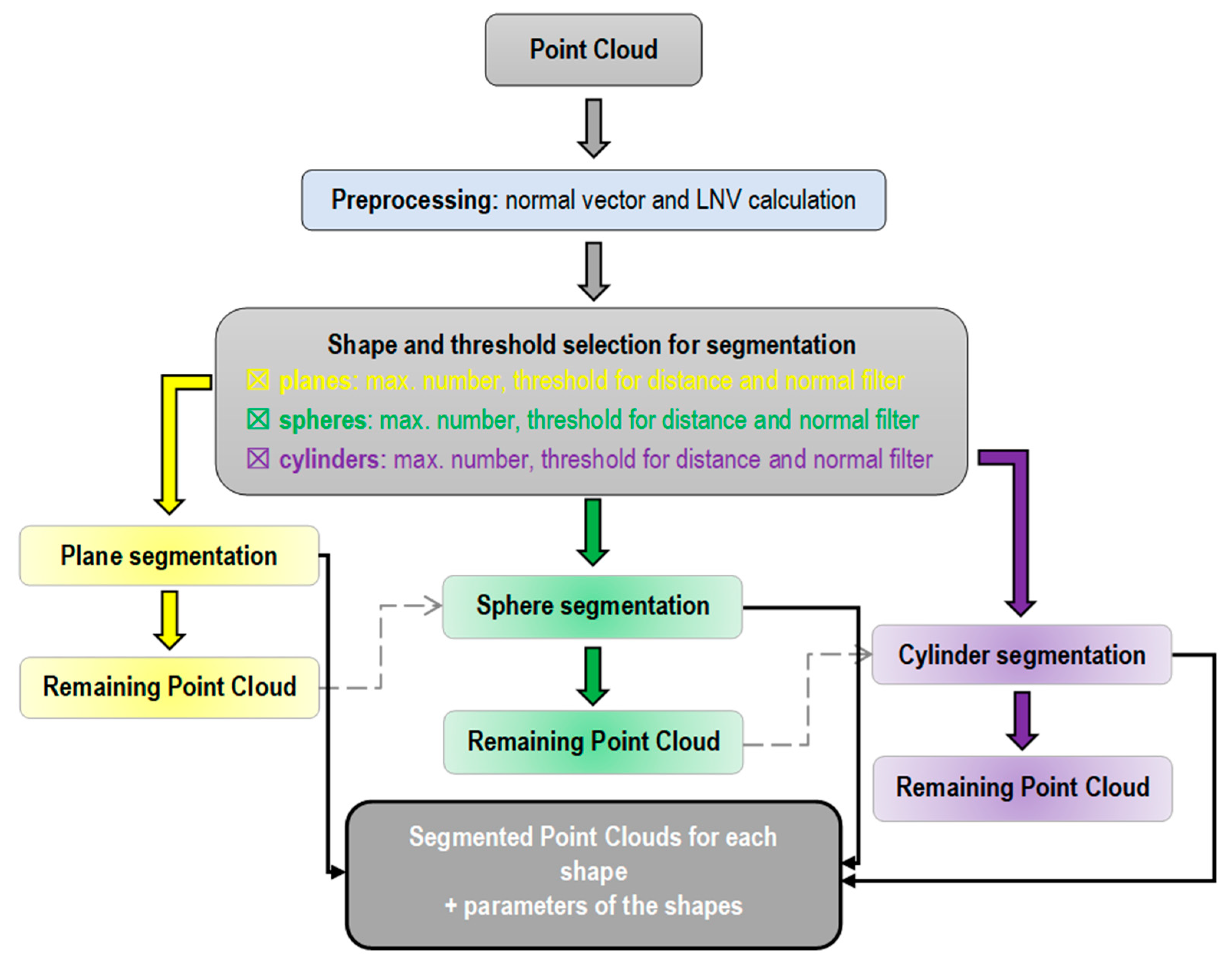
The following chapter proposes a robust algorithm for automated segmentation of geometric shapes (planes, spheres, cylinders) from point clouds. The proposed method can be applied to processing high-density point clouds. The algorithm process is shown in
Figure 1. The input data for the algorithm is a point cloud. The next step is selecting the type of geometric shapes for segmentation and threshold values.
With the algorithm developed, it is possible to perform segmentation of only the picked shapes (e.g., only planes, only spheres, only cylinders) or their combination. The threshold type is the same for all types of geometric shapes, but their value must be selected separately for each type. The mentioned threshold parameters are the assumed maximal number of a given shape in the point cloud and threshold values for the distance- and normal-based filtering. The meaning of each parameter will be explained in the related chapters.
In the case of segmentation of planes, spheres, and cylinders at once, the algorithm process is illustrated by the flowchart in
Figure 1. Before the segmentation procedure itself, some preprocessing steps are performed. First, the normal vectors at each point of the point cloud are calculated using small local planes, calculated from the 3D coordinates of the given point and the k-nearest neighbors. Orthogonal regression is used for plane estimation.
After the normal vectors are calculated, a new seed point selection technique is performed based on the local normal variation (LNV) value. The LNV value is estimated as the average value of the scalar products of the normal vectors from the
k-nearest points based on Equation (1):
where
is the absolute value of the scalar product of the normal vector at a given point and the normal vectors at the neighboring points.
Based on the LNV values at each point, it is possible to approximately determine the points where the occurrence of a planar surface is assumed (or, on the contrary, where a curved surface is expected to occur). Thus, points on a planar surface have LNV values close to zero, while points on a curved surface have higher values of LNV. In Equation (1), the LNV is calculated as a unitless parameter, but for better understanding and imagination, it is expressed in degrees in the following sections.
The whole segmentation procedure is divided into three main stages based on the shape types and is described in the following subsections.
2.2. Plane Segmentation
Of the three shape types, the task of plane segmentation is the simplest, so the algorithm starts with this task. The plane segmentation algorithm combines a modified RANSAC algorithm and the region-growing method.
The plane segmentation starts with the selection of the seed points. The seed point candidates are determined based on the proposed seed point selection technique. The selected seed points are the points where the value of LNV is the points where the value of LNV is less than 1° (i.e., the orientation of the normal vector at the given point is approximately parallel to the normal vectors at the k-nearest neighbors). This seed point is used as a starting point for the plane estimation. The first plane is estimated using the
nest nearest points. The number (
nest) of the nearest points depends on the local point density (LPD) at the selected seed point. In the proposed approach, this means selecting the points at a distance of 50 mm from the seed point. For the estimation of plane parameters, orthogonal regression is used, which minimizes the orthogonal distances to the estimated plane. The solution is based on the general equation of a plane (Equation (2)).
where
,
, and
are the parameters of the normal vector of the plane;
,
, and
are the coordinates of a point lying on the plane; and
is the scalar product of the normal vector of the plane and the position vector of any point of the plane.
First, the elements of the best-fit regression plane’s normal vector (
a,
b, and
c) from the selected points are calculated using singular value decomposition (SVD). Next, the parameter
d is calculated by substituting the coordinates of the center point and the elements of the normal vector into the rearranged form of the general equation of the plane (Equation (3)). These elements (
a,
b,
c, and
d) define the best-fit regression plane.
where
X0,
Y0, and
Z0 are the coordinates of the centroid point of the selected points for plane estimation.
Furthermore, the orthogonal distances of the points from the regression plane and the standard deviation of the plane estimation are calculated.
In the next step, the inliers for the given plane are identified (i.e., the points lying on the surface of the estimated plane) by testing the estimated regression plane against the nearest neighbors. Inlier selection is performed using two criteria:
distance-based criterion: only the points that are closer to the estimated plane than the selected threshold values are considered as inliers;
normal-based criterion: inliers are the points where the angle between the normal vector at a given point and between the normal vector of the regression plane is less than the threshold value.
The plane re-estimation and the inlier selection are performed iteratively, with a gradual increase in the number of the neighboring points tested. It is repeated until the number of points belonging to the plane stops increasing.
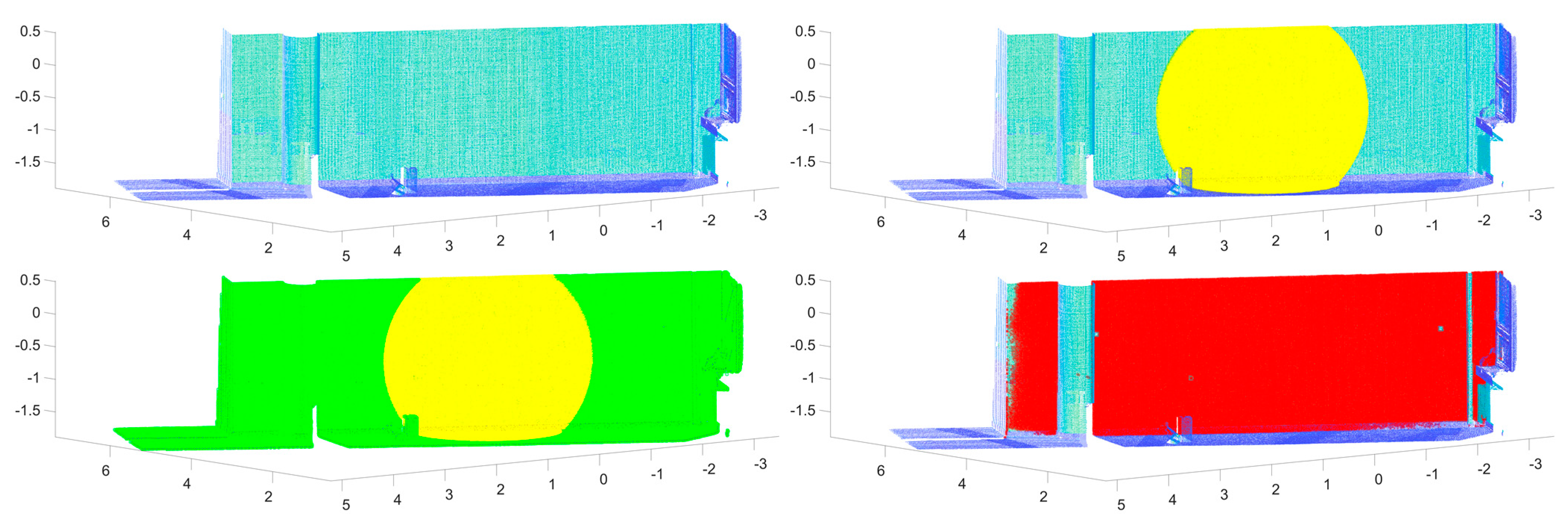
Figure 2 illustrates the plane segmentation process, where the initial point cloud (top-left) is shown (the points are colored by the intensity of the reflected measuring signal), then the approx. 102 thousand nearest points (top-right with yellow color) to the seed point, followed by the approx. 1.6 million nearest neighbors (bottom-left with green color), and with red color, the inliers for the given plane are shown (bottom-right).
Since the plane estimation strongly depends on the seed point selection and its neighborhood, it was necessary to introduce several validation steps to eliminate incorrect estimations. These validation steps are based first on determining whether there are enough inliers at each iteration, i.e., after the second iteration, at least two times more inlier points than the number of points from the first estimation (nest). It is expected that the number of inliers (points lying on the segmented surface) from the surroundings will increase gradually if the selected seed point lies on a planar surface. Then, it is determined whether the plane has sufficient point coverage. The local point density (LPD) value is calculated at each inlier point. In addition, the theoretical value of the LPD is calculated (if the plane has a uniform ideal coverage). The criterion is that at least 50% of the points need a higher LPD (with a certain tolerance) than the ideal LPD. This value (50%) was determined empirically based on testing the algorithm on several point clouds with various densities, complexities, and different levels of noise. This criterion is necessary in some cases, e.g., when processing a point cloud from an indoor environment of a building where there are several objects (e.g., furniture, PC accessories, etc.). In such cases, a plane can be estimated from some subsets of points that are lying on different objects (not lying on the planar surface), i.e., the result of the estimation can be a plane (though this plane is not a real one), since these points are from a separate dense subset of points lying on a surface of any object. The mentioned cases are eliminated from the estimation by this criterion.
If any of the validation steps are unsuccessful, the algorithm skips to the new segmentation cycle with a new seed point for a new plane candidate.
In most cases, the number of planes in the point cloud is not known in advance. Therefore, a technique is proposed to stop the calculation. The algorithm automatically breaks the calculation after segmenting all the planes located in the point cloud. If 100 incorrect segmentation attempts (incorrect attempt means that no plane is found at the selected seed point) are made in a row (after several successfully segmented planes), the calculation is stopped. In practical applications of the described algorithm on complex point clouds with several shapes (several plane-, sphere- or cylinder-shaped objects), the number of individual geometric shapes is usually not known in advance. Due to the higher level of automation, in the case of our algorithm, it is not necessary to enter the number of these shapes precisely. However, the algorithm automatically stops after these 100 incorrect attempts. The number 100 was also determined empirically, based on testing, but it can be adjusted based on the size and the complexity of the point cloud. Otherwise, if the number of planes in the point cloud is known, this number can be selected at the beginning of the algorithm, and the algorithm segments the chosen number of planes.
The results of the plane segmentation are the segmented point clouds for each plane and the parameters of the planes, which are: the parameters of the normal vector of the plane (a, b, c), parameter d, number of inliers, the standard deviation of the plane estimation (calculated from the orthogonal distances of the inlier points from the best-fit regression plane). After this part of the algorithm, further processing is performed only on the remaining point cloud (i.e., the points belonging to the segmented planes are excluded from the initial point cloud). This step indeed contributes to increasing the efficiency of the algorithm.
2.3. Sphere Segmentation
The data input into the sphere segmentation part are the remaining point cloud safter the plane segmentation, if plane segmentation has been performed (otherwise, it is the input point cloud). The part of the algorithm which has the role of the sphere segmentation is also partially inspired by the RANSAC algorithm. The least-square spherical fit is used to calculate the sphere parameter.
The process of the algorithm is similar to the plane segmentation algorithm. The first step is the selection of seed points based on the LNV values at each point (seed point candidates for spheres are the points where the LNV value is greater than 5°). This seed point selection technique significantly increases the efficiency of the algorithm. In cases of processing complex point clouds that contain several walls (planar surfaces, where the points have small local curvature—usually up to 5 degrees, because of undulation of the planar surface in some cases), with this step, the points lying on these surfaces are removed from the seed point candidates for sphere estimation. This technique is mainly for a rough removal of the points, where it is assumed that no sphere object can be found.
Then, the first approximate parameters of the sphere are calculated using the
nest number of nearest points to the selected seed point. The value of the
nest is calculated in the same way as in the case of planes. The estimation is based on a least-square spherical fit, which minimizes the perpendicular distances of the points from the sphere. The solution is based on the general equation of a sphere (Equation (4)).
where 𝑥, 𝑦, and 𝑧 are the coordinates of the points on the surface of the sphere,
,
, and
are the coordinates of the center of the sphere, and
r is the radius of the sphere.
By expanding Equation (4), we get the rearranged equation expressed in Equation (5):
Next, Equation (5) is represented in consolidated terms; which serves as an overdetermined system suitable for spherical fit. In this way, the approximate parameters of the sphere are obtained.
The iterative fitting and extraction process then uses the sphere’s approximate estimated parameters. Extraction, thus selecting the inliers for the estimated sphere candidate, is performed based on distance-based and normal-based filtration (similar to the plane segmentation part). In contrast to the plane algorithm, the extraction process is performed on the whole point cloud at once. The iterative re-estimation is performed until all the points of the detected sphere have been selected. The maximum number of iterations is set to 15. This number was determined empirically based on processing several point clouds with different complexity, noise, and number of spheres. However, this value is sufficiently oversized and was not reached in any of the mentioned tests due to several conditions to stop the calculation. It means that if no new point is added in 3 consecutive iterations, and there is no difference in the parameters of the sphere, the calculation is automatically stopped.
Moreover, several validation steps were proposed. The first was based on inlier number (whether there are enough inliers for the selected seed point—at least twice more inliers than the value of nest after the fourth iteration). The next was based on the convergence of the sphere parameters. Therefore, the differences in the estimated parameters of the sphere are determined in two consecutive iterations (after the fifth iteration), and the convergence parameter gives the maximum allowed difference (). The last validation step ensures that the standard deviation of the spherical fit is not greater than the specified parameter. The standard deviation is estimated based on the orthogonal distances of the inliers from the sphere surface. If any of these validations are unsuccessful, the algorithm skips to a new segmentation cycle with a new seed point. The proposed technique to stop the calculation automatically is also included in this part (sphere segmentation part) of the algorithm.
The results are the segmented point clouds and the parameters for each shape (sphere parameters [cx, cy, cz, r], inlier number, the standard deviation of the sphere fitting). The segmented clouds for each sphere are also excluded from further processing.
From experiments (processing of several point clouds containing sphere objects), it was found that coverage of only approximately 40–50% of the scanned sphere surface (e.g., when scanning only from a single position of the instrument) is sufficient for extraction of the sphere with the algorithm depicted. However, a certain LPD is needed, i.e., at least 100 points are required to be homogeneously distributed on the scanned part of the sphere surface.
2.4. Cylinder Segmentation
The last part is for cylinder segmentation, which is the most complex. The algorithm developed for cylinder segmentation can be categorized into model-based methods and is partially based on the elements of the Hough transform. Similar to the sphere segmentation part, the input data is only the remaining point cloud if the segmentation of other geometric primitives has been performed.
The sequence of the processing steps is similar to the plane and sphere segmentation algorithms. The algorithm starts with selecting seed points based on the calculated LNV values (the seed point candidates are the points where the LNV is greater than 3°). Next, the first cylinder is estimated from the
nest number of closest neighbors to the seed point. The value of the
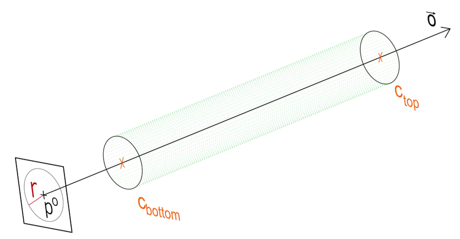
nest is calculated in the same way as in the case of planes and spheres. The estimated cylinder parameters are illustrated in
Figure 3.
The cylinder estimation is divided into four main steps:
Computing the cylinder axis orientation ()—vector, perpendicular to the normal vectors in nest closest neighbors.
Projection of these points onto a plane that is orthogonal to the cylinder axis (). If the selected points lie on the cylinder’s surface, they are distributed in a circle.
Estimating the projected circle parameters (i.e., coordinates of the circle’s center and radius). This estimation uses algebraic fitting, where algebraic distances are minimized [
36]. The coordinates of the circle’s center point are considered as the point
po, which lies on the cylinder axis. The radius of the estimated circle equals the radius of the cylinder shell.
Computation of the base centers of the cylinder (top and bottom base center points). First, the distances between the inliers and the center point of the cylinder axis are calculated according to Formula (6). The maximal and minimal distances are then determined from the vector . These values are then substituted into the Formula (7) to calculate the coordinates of the top and bottom base centers.
where
p is the vector containing the 3D coordinates of the inlier points,
and
are the coordinates of the center points of the top and bottom bases of the cylinder.
The estimation steps described above are applied iteratively for the inlier points. The set of points considered as inliers is updated at each iteration based on two criteria, mathematically formulated as follows:
where Δ
disti is the orthogonal distance between the selected point and the cylinder surface, Δ
normi is the angle between the normal vector of the selected point and the vector that is perpendicular to the cylinder axis
in the selected point. The parameters
and
are the selected threshold values. The threshold parameter for the distance-based filter is chosen as a percentage of the radius of the cylinder, as the point cloud may contain several cylinders with different radii.
Based on the criteria in Equation (8), the inliers are automatically updated in every iteration, and the outliers are removed from the estimations. After every iteration, the cylinder parameters are re-estimated using all the inliers that meet the specified conditions. The inlier updating is performed on the whole point cloud at once, similar to the sphere segmentation part.
The iterative re-estimation is performed until all the points of the detected cylinder have been selected, and the maximum number of iterations is set to 15. In this case, several validation steps were also proposed. They are based on inlier numbers (similar to the planes and spheres) and parameter convergence (similar to the spheres). Furthermore, a novel validation step based on cylinder coverage was proposed. In this validation method, the cylinder shell is first transformed into a plane, then divided into a grid (the size of the grid is determined automatically based on the dimensions of the cylinder), and the number of points in each cell of the grid is determined. Next, a cell’s ideal average density (in the case of an evenly covered cylinder surface with inliers) is computed. The value of the ideal density is estimated based on the known dimensions of the cylinder, the known size of the grid, and the known number of inliers. If at least 25% of the cells have ideal coverage, the cylinder is considered a reliable one.
The method of automatically stopping the calculations is also included in this part of the algorithm, as in the case of planes and spheres. The results are the segmented point clouds and the parameters (a point on the cylinder axis po, the orientation of the cylinder axis , the radius r and the height h of the cylinder shell) for each identified cylinder.
2.5. Development of a Standalone Application for Automation of the Segmentation Process
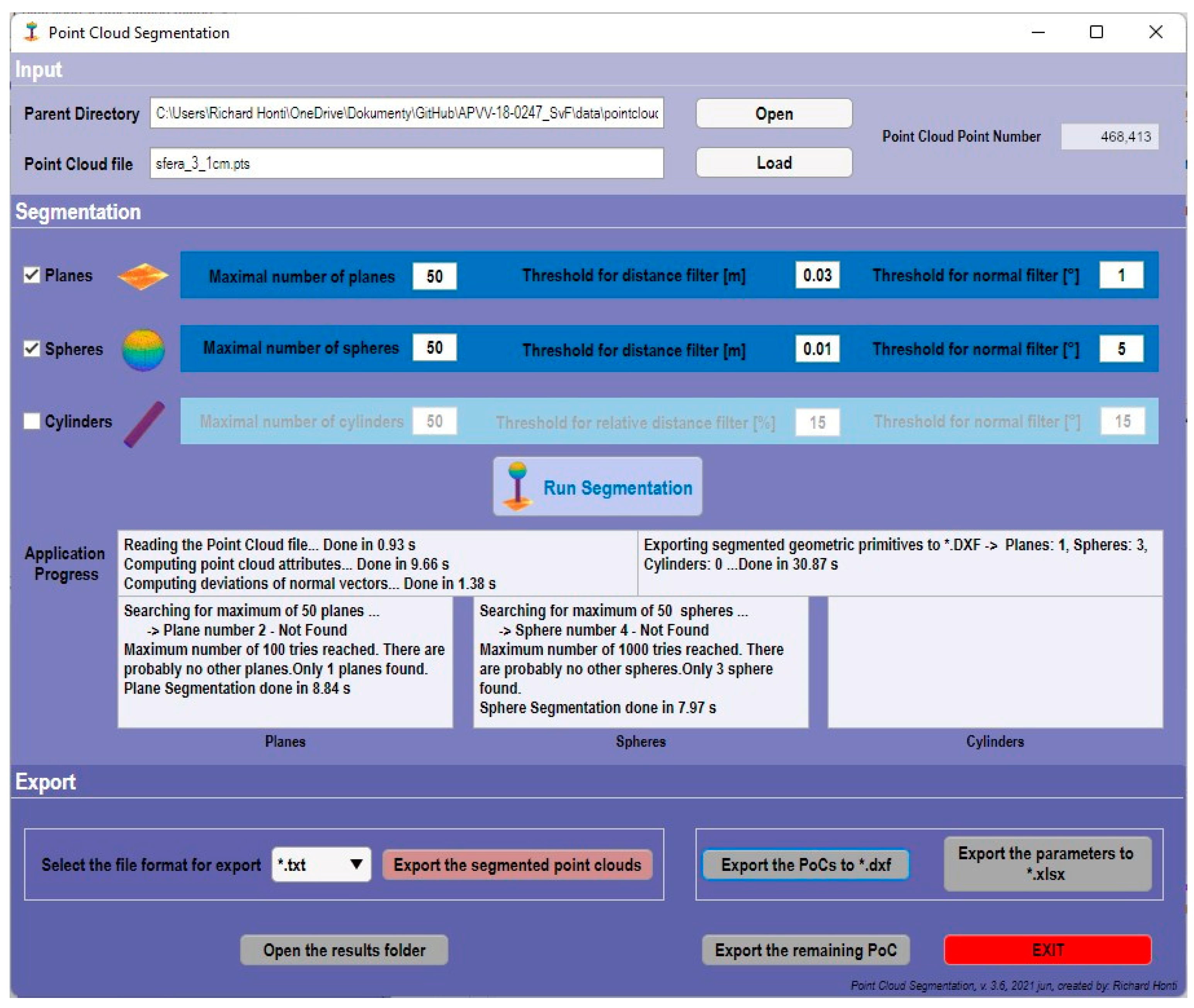
A standalone computational application (
PoCSegmentation) was developed to simplify and automate the segmentation procedure. The application’s graphical user interface (GUI) was designed in MATLAB
® software. Also, the calculation takes place in the MATLAB
® software environment, so the Matlab Runtime is required to run the application, which is freely available. The dialogue window of the application (
Figure 4) consists of three major sections. The top section is for importing the point cloud. The point cloud can be imported in several file formats, which are as follows: *
.txt, *
.xyz, *
.pts. *
.pcd, *
.ply, *
.mat.
The middle part serves for the segmentation itself, where at the top the types of geometric shapes can be chosen, and the threshold parameters can be selected. The segmentation procedure is started by pressing the Run Segmentation button. At the bottom of this section, the application’s progress is described, i.e., the individual processes executed step by step and the time required for its execution. The bottom part of the dialog window is used to export the segmentation results. The PoCSegmentation application offers various options to export the results. On the left, the segmented point clouds can be exported in several file formats (*.txt, *.pts, *.xyz, *.pcd, *.ply, *.mat). In addition, it is also possible to export the segmented point clouds into *.DXF (Drawing Exchange Format), which is a CAD data file format for vector graphics, and which can be imported into more than 25 applications from various software developers. The advantage of the application is that, in the DXF file, the individual segmented point clouds are divided into separate layers. Next, the parameters of the geometric shapes can be exported to an Excel file, and the remaining point cloud can also be exported to *.pts format.
2.6. Testing of the Proposed Approach
Experimental testing of the
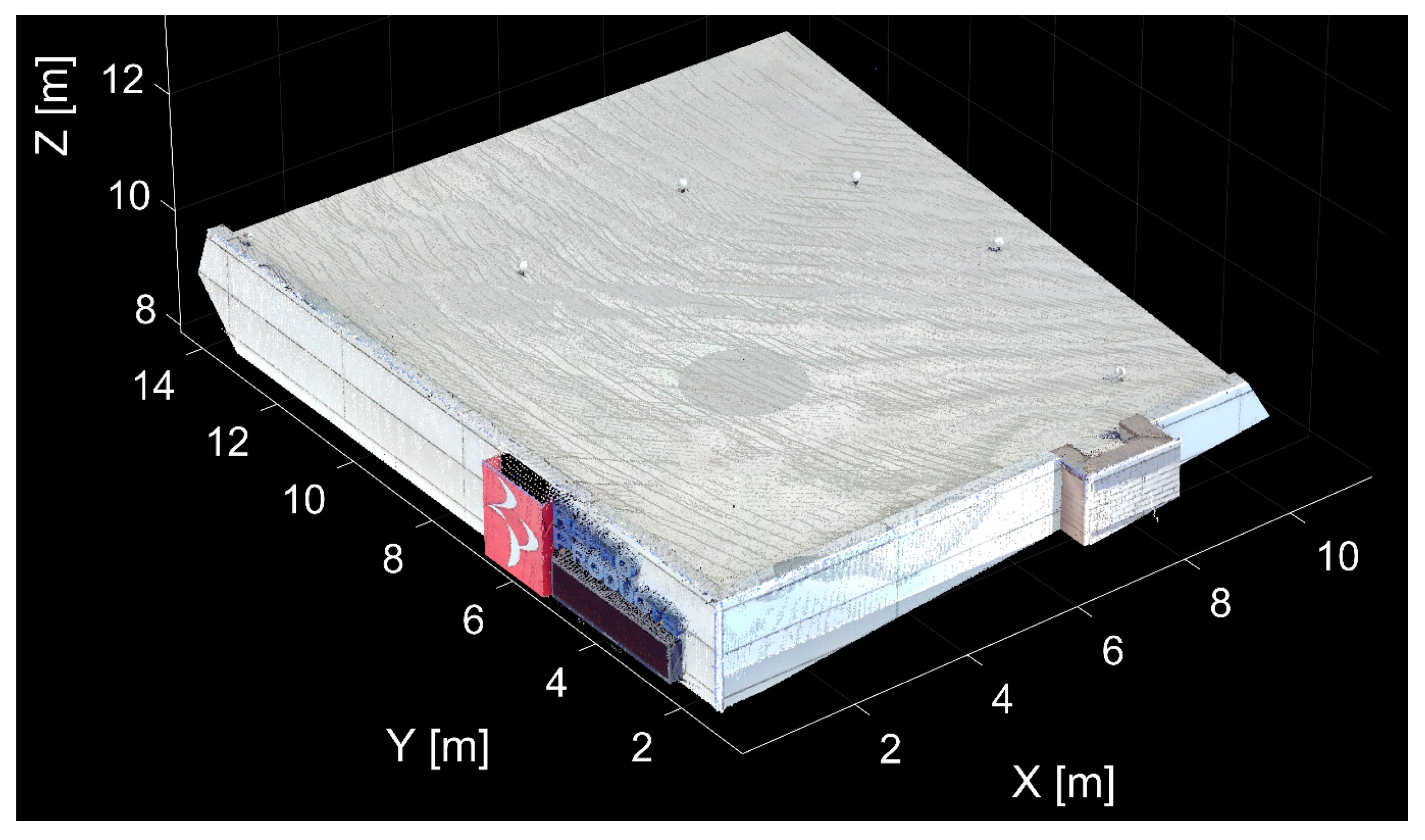
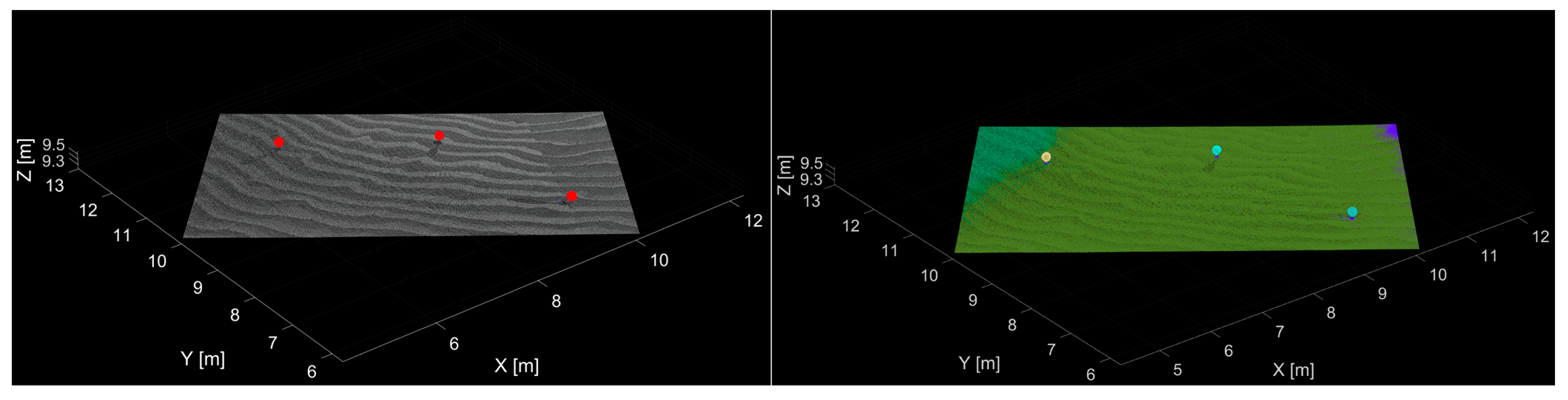
PoCSegmentation application, implemented based on the algorithm proposed, was performed on several point clouds with various densities, complexities, and different levels of noise. For the first experiment, a point cloud from an industrial building (Point Cloud No. 1) (
Figure 5) was used that contained 12 planar surfaces and 6 sphere objects. The mentioned point cloud was obtained from an online point cloud database accessible at [
37].
The initial point cloud contained approximately 815 thousand points. In this case, the threshold values were chosen as follows: the shapes for segmentation were planes and spheres, the threshold for the distance filter was 0.050 m for the planes and 0.020 m for the spheres, and the threshold for the normal-based filter was 5° for the planes and 10° for the spheres. The developed application segmented 13 planes and six spheres (reference sphere targets).
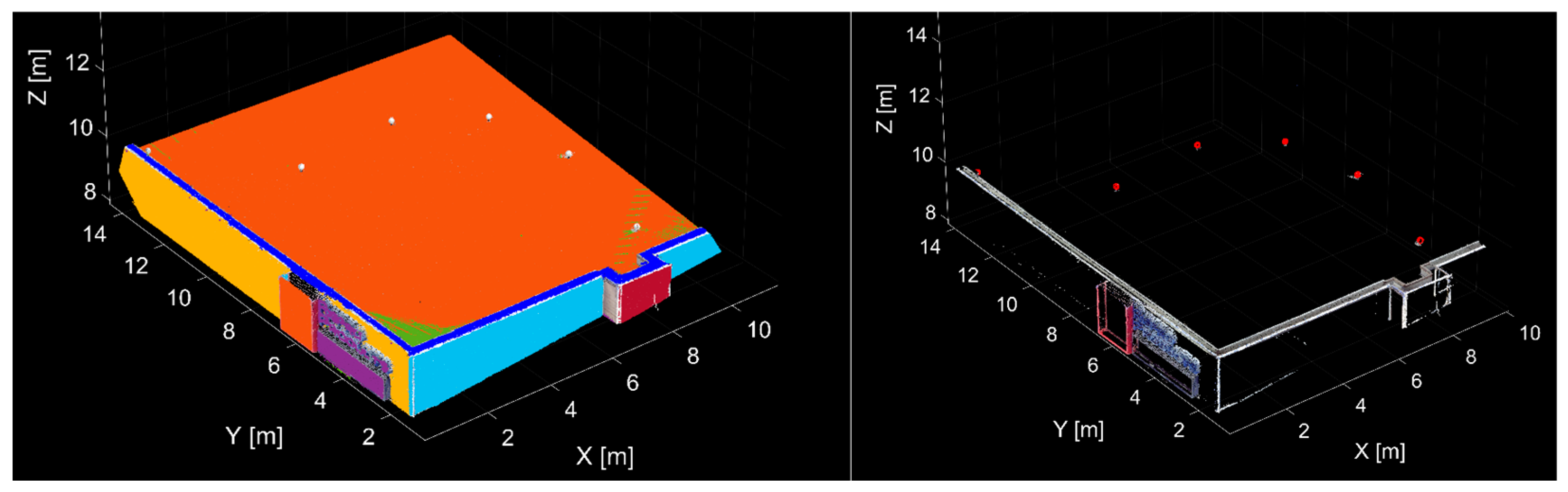
The results of the segmentation process are shown in
Figure 6. The left side of
Figure 6 shows the segmented points of the individual planes differentiated by color, and on the right, the points of the segmented spheres are shown in red color. To verify the results of sphere segmentation, the differences among the known parameters (radius of the sphere targets are defined by the producer of the targets) and the estimated parameters from the application were calculated. The differences were below 1.2 mm in any case.
The scanned object contained 12 planar and six spherical surfaces. Using the developed application, 13 planes and six spheres were automatically segmented. However, the difference in one plane is not caused by the imperfection of the algorithm but by the undulation and the bumpy surface of the roof of the building. The algorithm divided the roof into two parts while, based on the selected threshold values, some points of the roof did not belong to the plane shown in orange.
After segmenting the depicted planes and spheres, the remaining point cloud represented only 8% of the points from the initial point cloud. These points were mostly the edges of the individual planes and points on the mounting pads for the spherical targets, so the points did not belong to any plane or sphere.
The entire segmentation procedure (13 planes and six spheres) was executed in approximately 8 min on a PC with the following basic parameters: operating system—Windows 10 Pro, CPU—Intel Core i7 9700F Coffee Lake 4.7 GHz, RAM—32.0 GB DDR4, Motherboard—MSI B360 Mortar, Graphics—NVIDIA GeForce RTX 2070 SUPER 8 GB, SSD—WD Blue SN500 NVMe SSD 500 GB.
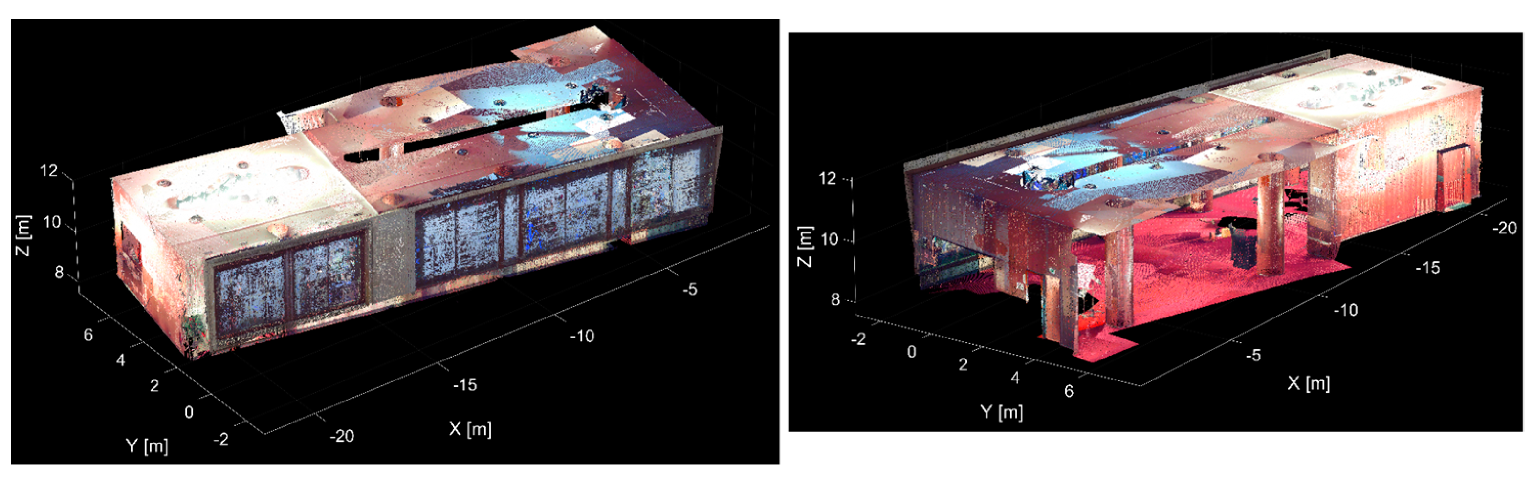
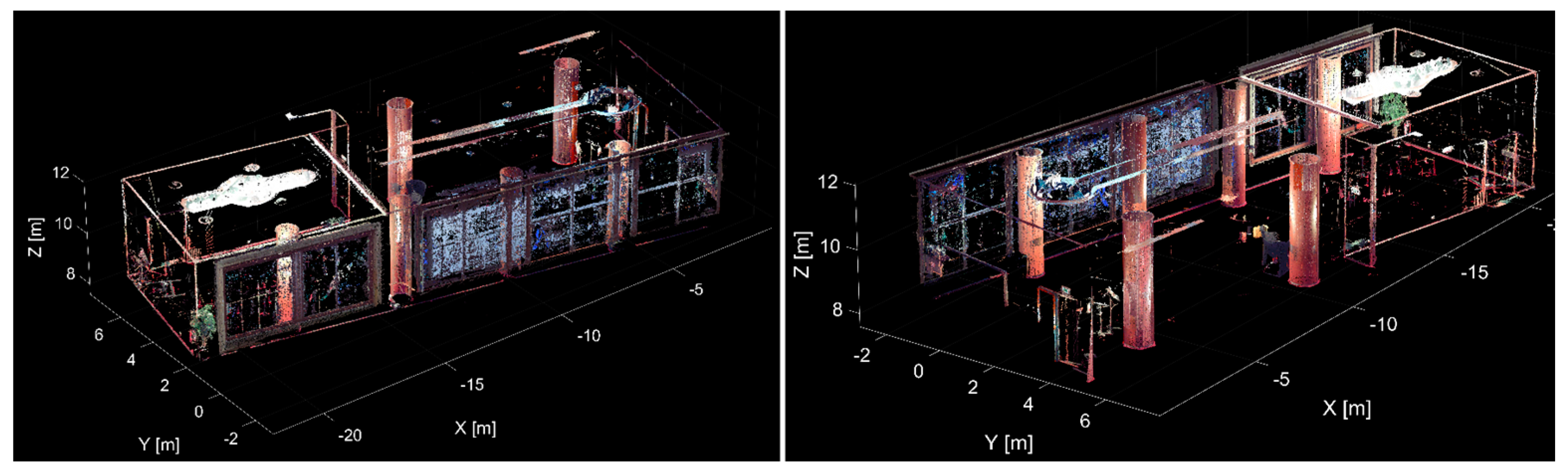
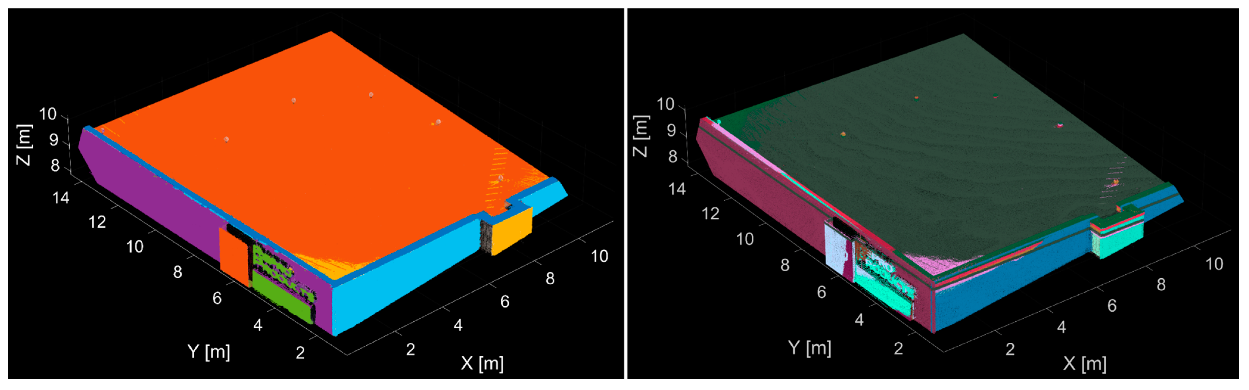
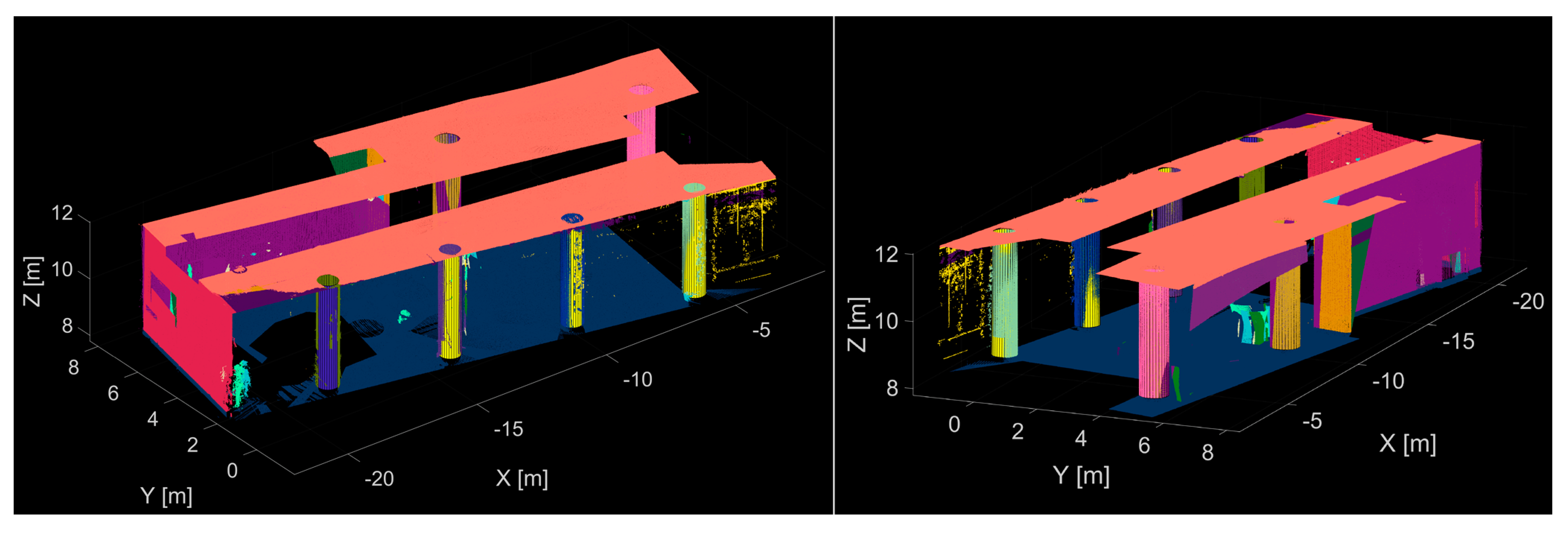
In the next test, the point cloud of a chosen room of the Pavol Országh Hviezdoslavov Theatre in Bratislava was used (Point Cloud No. 2), which contained more than 1.8 million points. Scanning was also performed with a Trimble TX5 3D laser scanner. The average point cloud density was 2 cm, and the accuracy in the spatial position of a single measured point was less than 5 mm. The initial point cloud from two views is shown in
Figure 7.
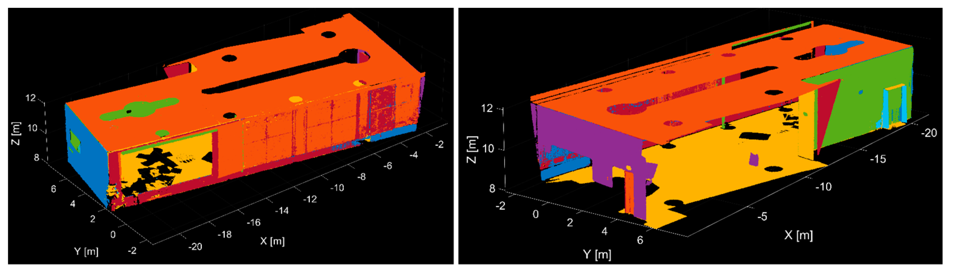
The scanned room contained 22 planar surfaces (walls, floor, etc.) and six cylinder-shaped columns. The threshold values for segmentation were as follows: for the distance-based filter, 0.020 mm for the planes and 15% (of the estimated radius) for the cylinders; for the normal-based filter, 2° for the planes and 15° for the cylinders. The algorithm identified and segmented 22 planes and six cylinders from the point cloud. The result of the plane segmentation is shown in
Figure 8, where the individual planes are differentiated by color.
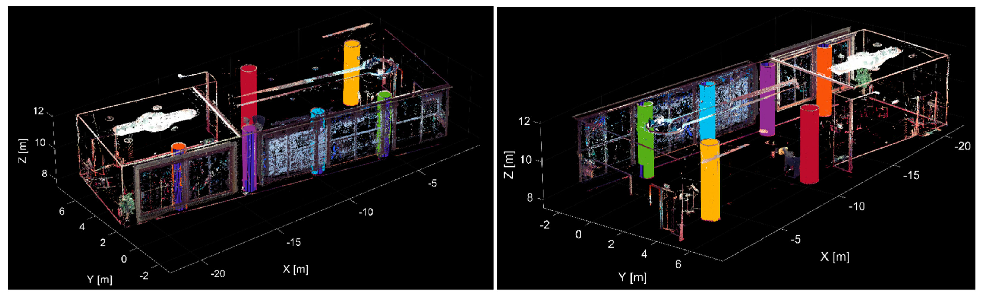
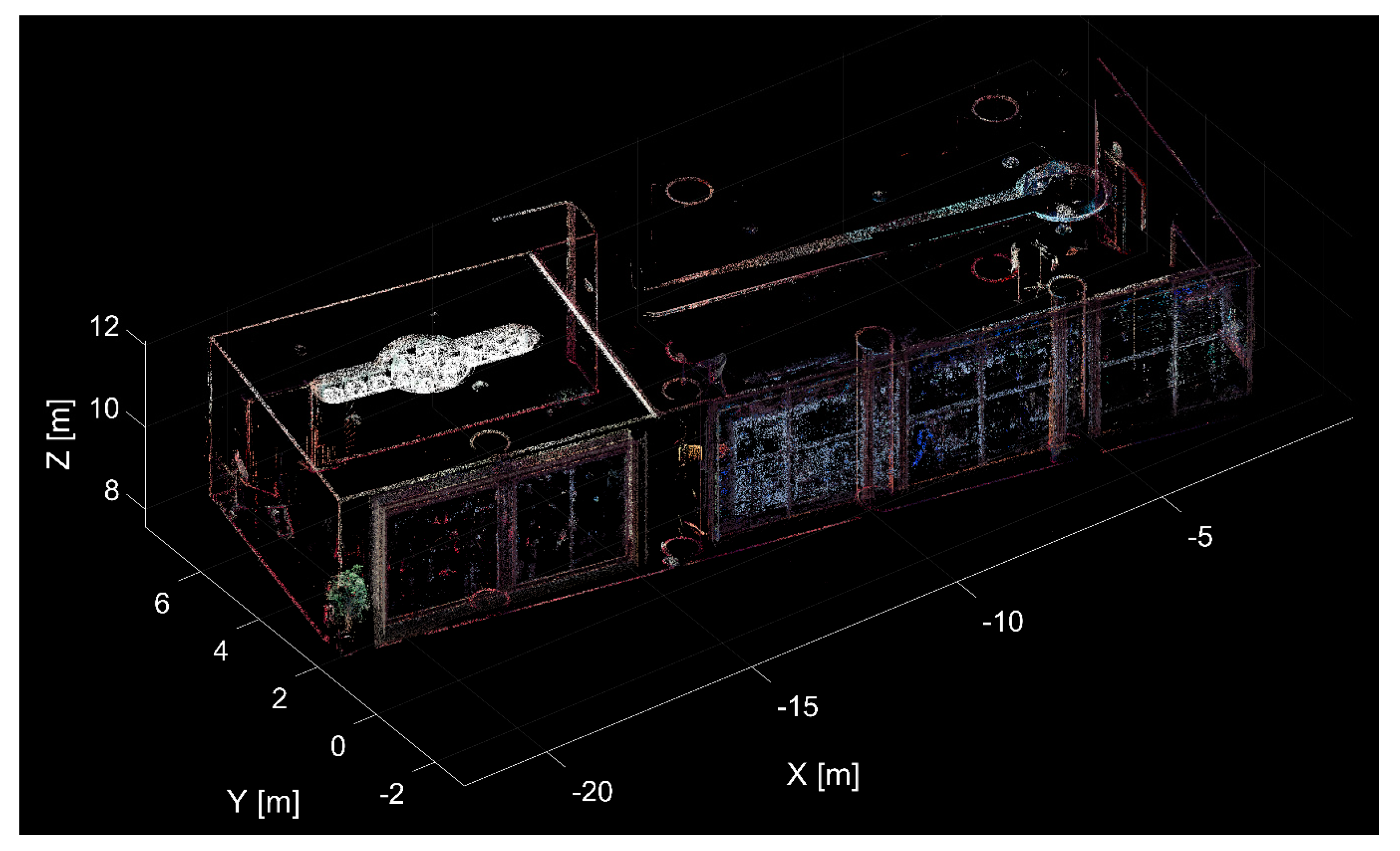
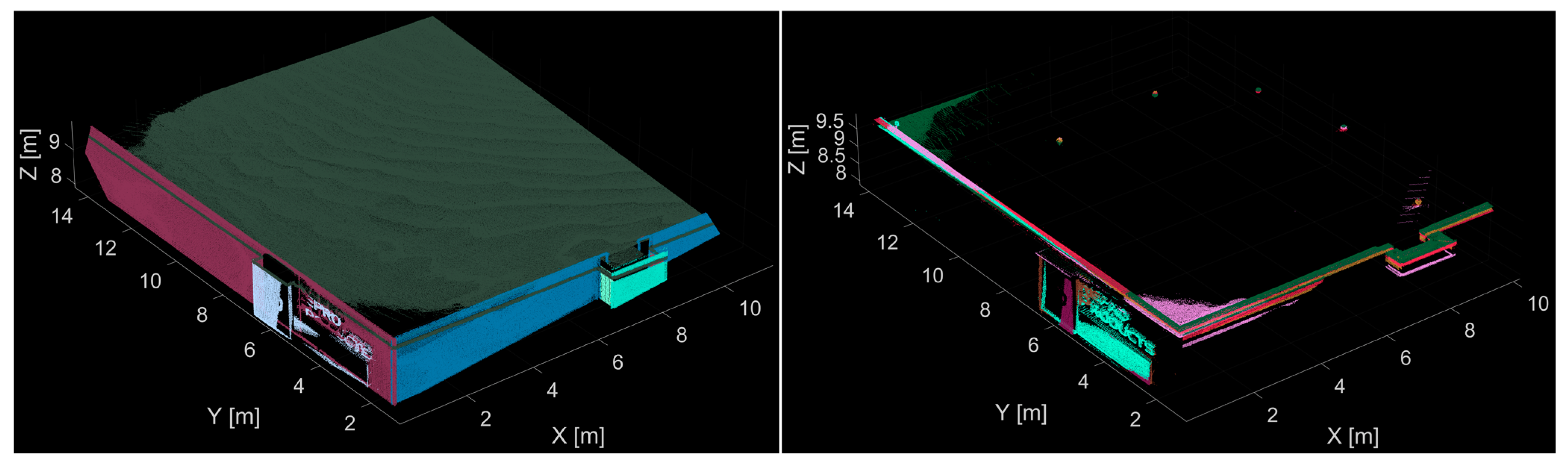
Figure 9 shows the remaining point cloud after the plane segmentation since, after the individual planes are segmented from the point cloud, they are removed from further processing. The noted point cloud represents only 34% of the initial point cloud, so in the next step of the algorithm, that is, cylinder segmentation, the processing is performed on a much smaller set of points.
Figure 10 shows the remaining point cloud after the plane segmentation with the segmented cylinders, which are differentiated by color. With the mentioned threshold values, segmentation of 6 cylinders was performed.
To verify the results of cylinder segmentation, the known (real) parameters of individual cylinders were compared with the estimated parameters from processing the point cloud with the application developed. The cylindrical columns had a uniform radius (r
real) of approximately 0.400 m and a height (h
real) of approximately 3.900 m. The parameters of each of the columns were measured by a measuring tape at various positions, and the final parameters were calculated as average values. The radiuses (r
app) and heights (h
app) obtained from the processing are shown in
Table 1 with the calculated absolute deviations. The maximal deviation in radiuses was 9 mm and in height was 9 mm. In these deviations, the imperfection of the construction of these columns, the effect of the environmental conditions, the systematic errors of the instrument, the measurement error, and the processing errors (the standard deviation (
in
Table 1) of the cylinder fitting to the segmented points was 10 to 15 mm at the mentioned threshold values) are also included.
Figure 11 shows the remaining point cloud after segmenting 22 planes and six cylinders. These points are on the edges of the individual shapes and objects in the room (e.g., parts of the room, lightning, flowerpots with plants, chairs, tables, etc.). The remaining cloud represents only 15% of the initial point cloud.
Using the proposed application, all the planes and cylinders that form the room’s structural elements (walls, columns, etc.) were correctly and automatically detected and segmented from the point cloud.
The segmentation procedure (22 planes and 6 cylinders) was executed in approximately 11 min on the same PC, as in the first test case.
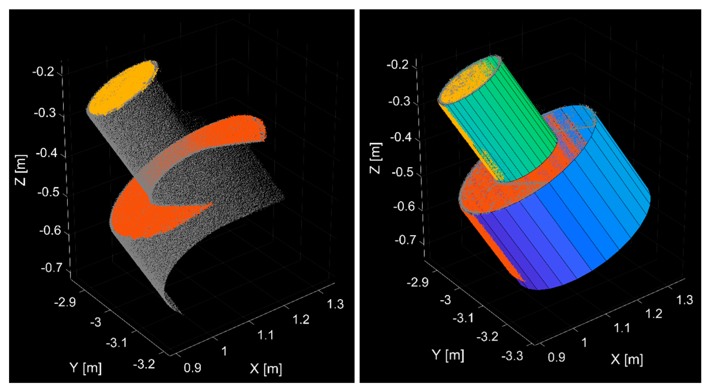
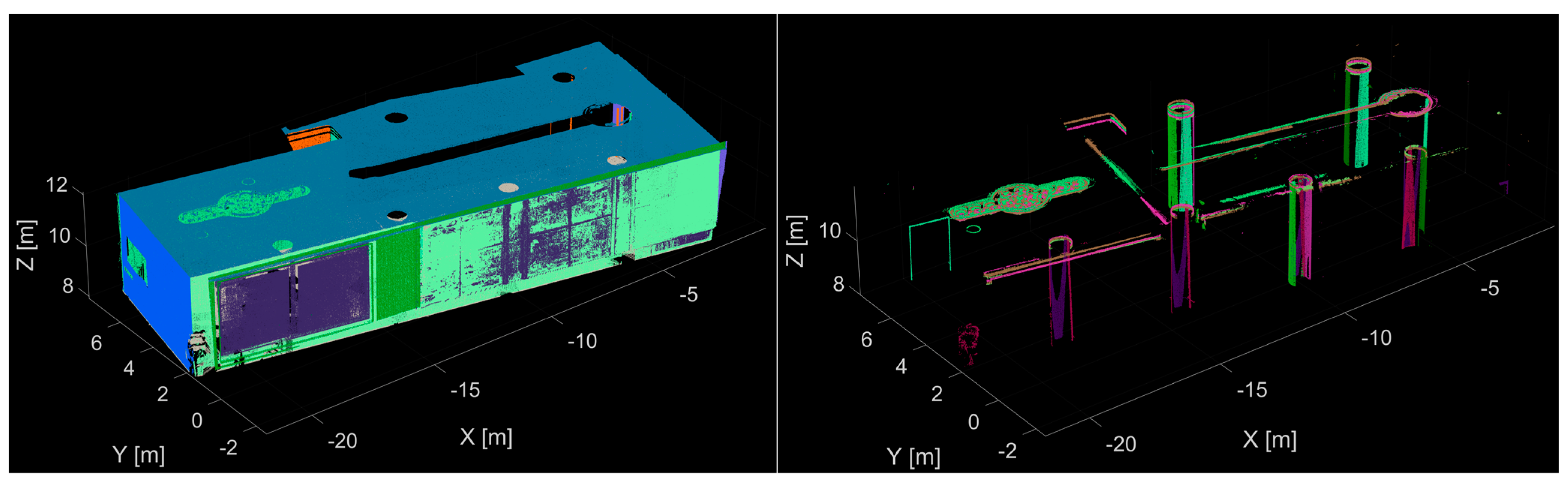
The last test was performed on a point cloud of the double-cylinder-shaped test object (Point Cloud No. 3). The measurement was performed with TLS Leica Scanstation 2 (average density 1 cm, the accuracy of a single measured point up to 2.5 mm, approximately 202 thousand points). The threshold values for segmentation were as follows: the threshold for the distance-based filter was 10 mm for the planes and 10% for the cylinders, and the thresholds for the normal-based filter were 0.5° for the planes and 5° for the cylinders.
Figure 12 shows the segmentation result; on the left side, the two segmented planes are shown, and on the right side, the two segmented cylinders are shown.
In this case, the differences between the known geometric parameters (radius and height of the cylinders) and the estimated parameters from the processing were also calculated to verify the cylinder estimation (
Table 2). The geometric parameters of the cylinder object were measured by a CMM (Coordinate Measuring Machine) measuring system with an accuracy of 0.1 mm. The radius differences were 0.2 mm for the larger cylinder and 0.1 mm for the smaller cylinder. The height differences were 0.3 mm for the larger cylinder and 0.5 mm for the smaller cylinder.
The whole segmentation procedure (2 planes and 2 cylinders) was executed in less than 1 min on the same PC, as in the case of the first two tests.
4. Conclusions
Data acquisition is almost fully automated with the currently available laser scanners. Measurement can be performed relatively easily and in a short time. However, manually processing the measured point clouds can be time-consuming and complicated. Therefore, a basic premise of the efficiency of using point clouds is a high degree of automation of the processing steps. For example, when creating a 3D model (or BIM) of an existing building, one of the basic steps is the identification and segmentation of the basic structural elements of the object. In most cases, these basic elements are formed in the shape of basic geometric primitives (e.g., walls—planes; columns or piping network—cylinders; etc.). Therefore, automation of identification and segmentation of sphere objects can be useful, for example, in the case of point cloud registration based on spherical targets, and it also simplifies the 3D model creation.
The paper describes the algorithm proposed for automated identification and segmentation of geometric shapes from point clouds with the requirement of selecting a minimal number of input parameters. The algorithm can detect end-segment subsets of points belonging to planes, spheres, and cylinders from complex, noisy, unstructured point clouds. Inlier detection is performed using distance-based and normal-based filtering. Additionally, several validation steps were proposed to eliminate incorrect estimations. The algorithm proposed was tested on several point clouds with various densities, complexity, and different levels of noise. Specifically, testing on three different point clouds was described, one containing planes and spheres and two other point clouds with planes and cylinders. In all cases, the proposed algorithm correctly identified the geometric shapes regardless of their size, number, or complexity. Moreover, one of the most significant advantages of the algorithm is that the results can be exported directly to DXF exchange format for further processing. Besides that, comparison between the proposed algorithm and the standard RANSAC algorithm was performed separately for the individual geometric shapes on several point clouds. On average, the segmentation quality was increased from 50% to 100% with the described algorithm.
A standalone application that enables semi-automation of the point cloud segmentation procedure is developed in MATLAB® software. However, for its execution, the Matlab Runtime is necessary. In the future, approaches for the identification and segmentation of free-form objects from point clouds will be proposed and programmed.


