Author Contributions
Conceptualization, F.G., J.X. and R.L.; data curation, A.H.; formal analysis, F.G.; Funding acquisition, F.G. and J.W.; investigation, F.G. and J.X.; methodology, F.G., J.X. and H.Z.; project administration, F.G. and J.W.; resources, F.G., J.W. and H.Z.; software, F.G., J.X. and R.L.; supervision, F.G. and R.L.; validation, F.G., R.L.; visualization, F.G., J.X. and A.H.; writing—original draft, F.G. and J.X.; writing—review and editing, F.G. and H.Z. All authors have read and agreed to the published version of the manuscript.
Figure 1.
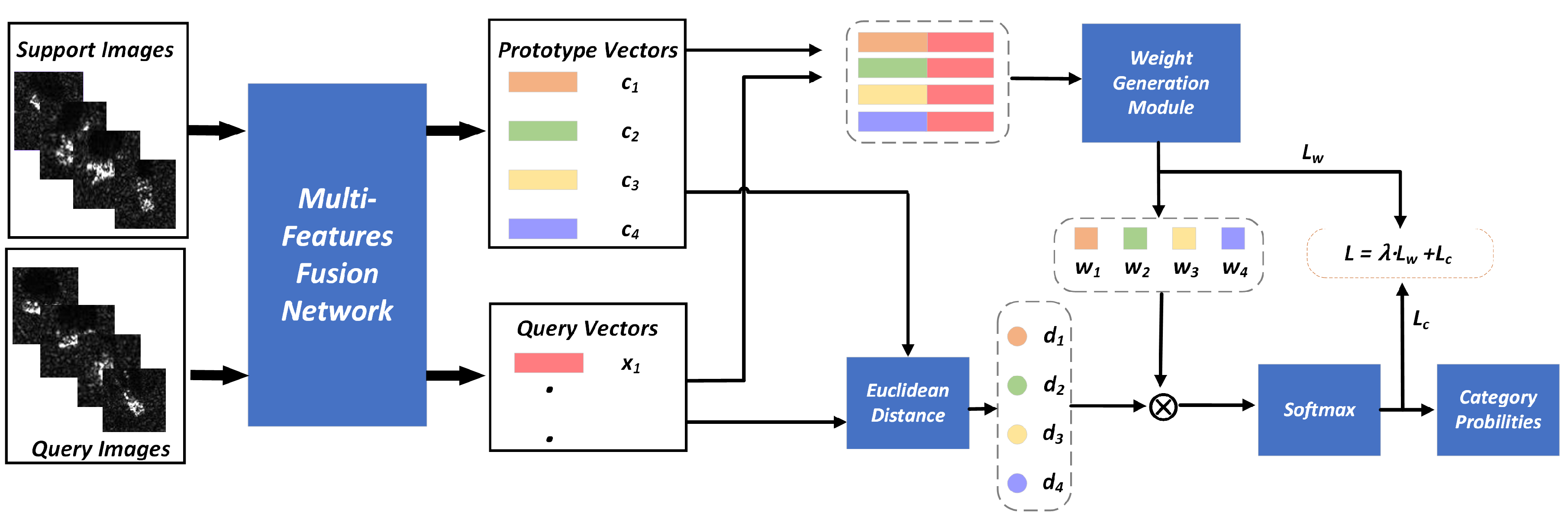
The framework of our proposed few-shot SAR image recognition method. The whole structure can be divided into two parts: the feature extraction network (MFFN) and the weighted Euclidean distance classifier. Support images are fed into the MFFN to extract features and then calculate the prototypes by averaging. Query feature vector is extracted by MFFN to calculate the corresponding Euclidean distance . Afterwards, is concatenated with the prototypes , and the concatenation vectors are sent to the weight generation module to calculate weights . Finally, the weighted distances are obtained by multiplying weights with the Euclidean distance, and the softmax function is adopted to calculate the category probabilities on the weighted distances.
Figure 1.
The framework of our proposed few-shot SAR image recognition method. The whole structure can be divided into two parts: the feature extraction network (MFFN) and the weighted Euclidean distance classifier. Support images are fed into the MFFN to extract features and then calculate the prototypes by averaging. Query feature vector is extracted by MFFN to calculate the corresponding Euclidean distance . Afterwards, is concatenated with the prototypes , and the concatenation vectors are sent to the weight generation module to calculate weights . Finally, the weighted distances are obtained by multiplying weights with the Euclidean distance, and the softmax function is adopted to calculate the category probabilities on the weighted distances.
Figure 2.
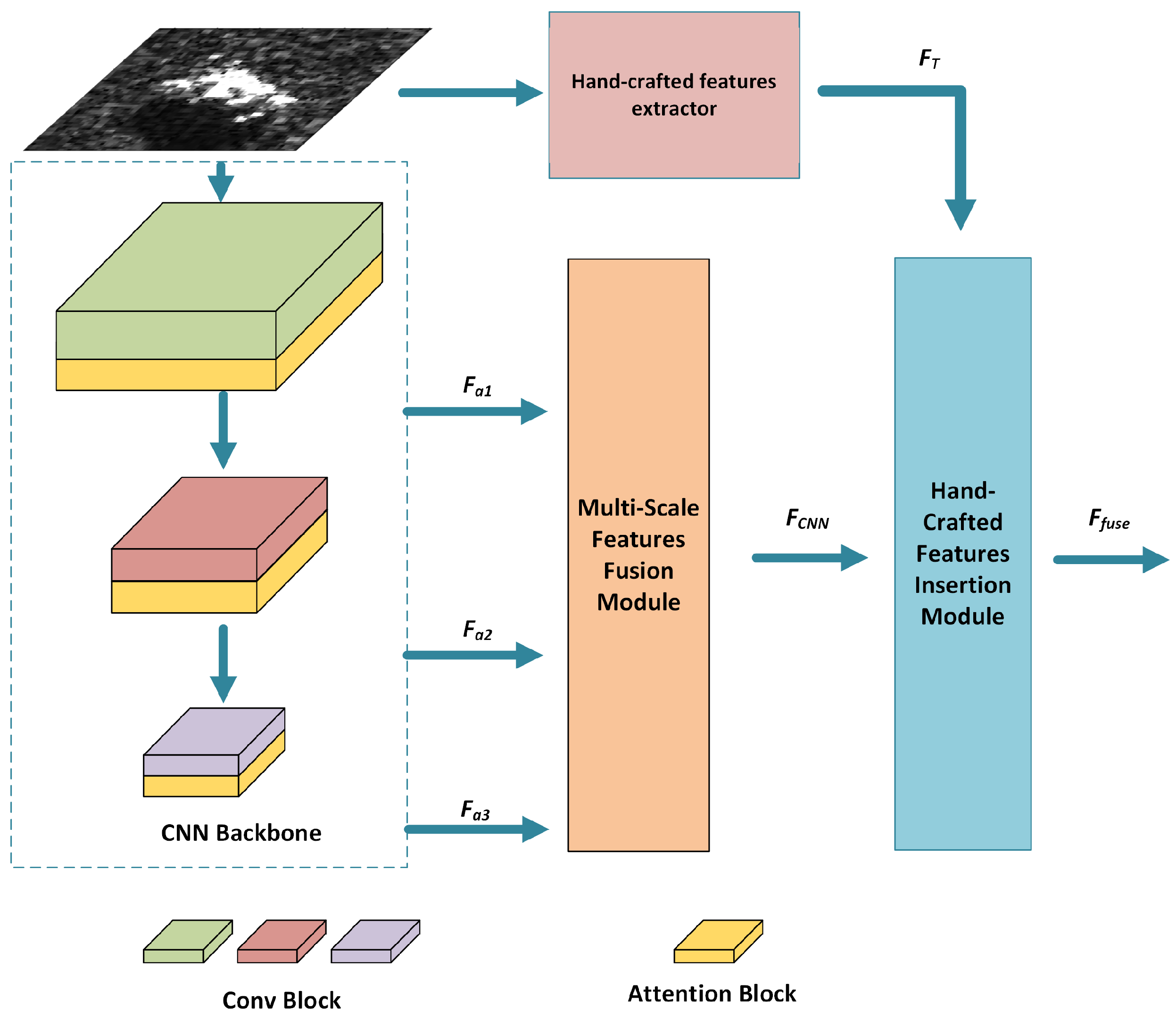
The overall architecture of the MFFN includes the MsFFM and the HcFIM. The channel-optimized features with different scales are fed into the MsFFM to utilize the complementary information from different layers. Afterwards, the fused feature is combined with the traditional hand-crafted features in the HcFIM. denotes the final output feature of the MFFN.
Figure 2.
The overall architecture of the MFFN includes the MsFFM and the HcFIM. The channel-optimized features with different scales are fed into the MsFFM to utilize the complementary information from different layers. Afterwards, the fused feature is combined with the traditional hand-crafted features in the HcFIM. denotes the final output feature of the MFFN.
Figure 3.
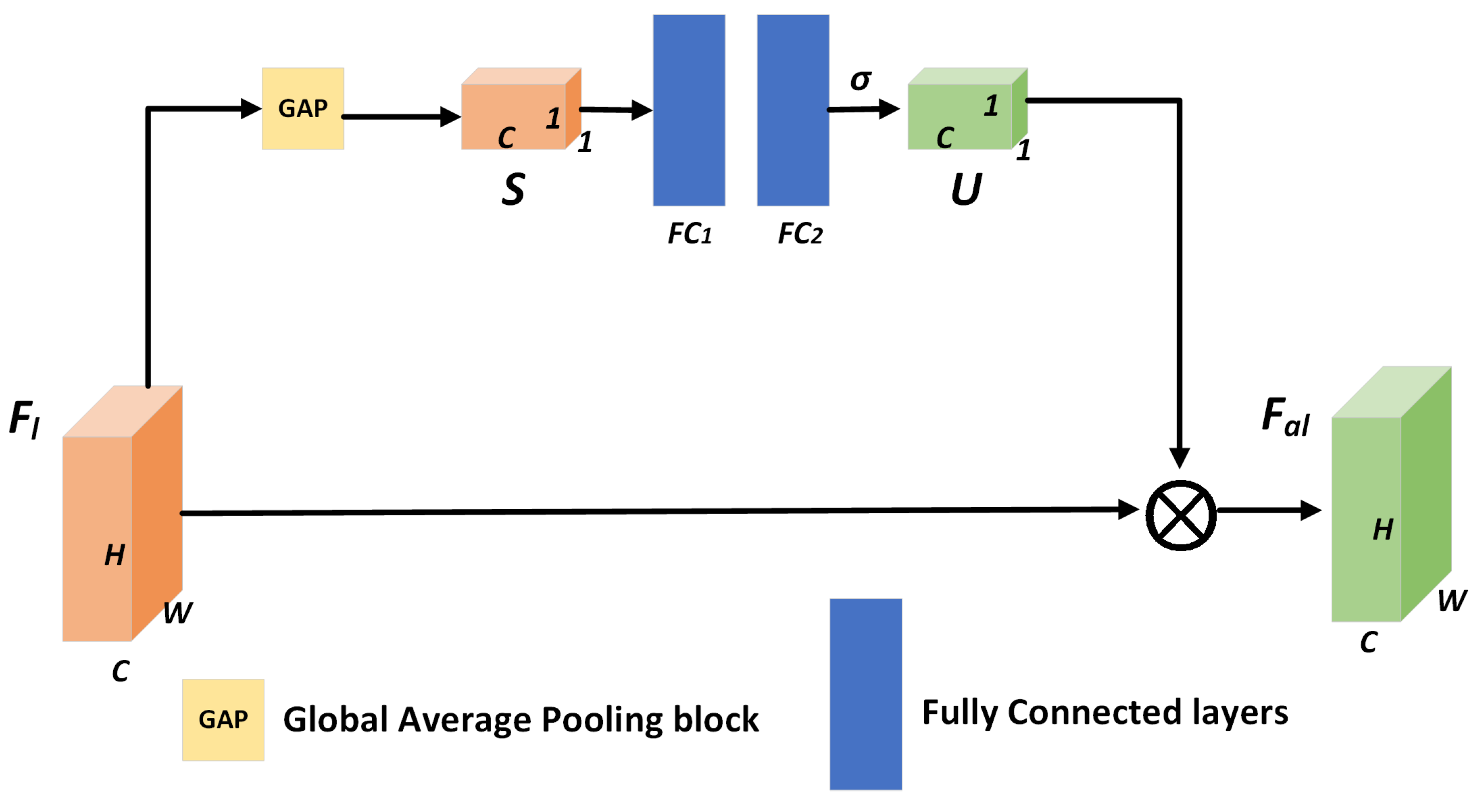
The operation process of the SE-Net. The channel descriptors are first generated by global average pooling, then the attention values are calculated by the fully-connected layers. Finally, the channel-refined features can be calculated by performing channel-wise multiplication. represents the channel-wise multiplication operation and denotes the sigmoid function.
Figure 3.
The operation process of the SE-Net. The channel descriptors are first generated by global average pooling, then the attention values are calculated by the fully-connected layers. Finally, the channel-refined features can be calculated by performing channel-wise multiplication. represents the channel-wise multiplication operation and denotes the sigmoid function.
Figure 4.
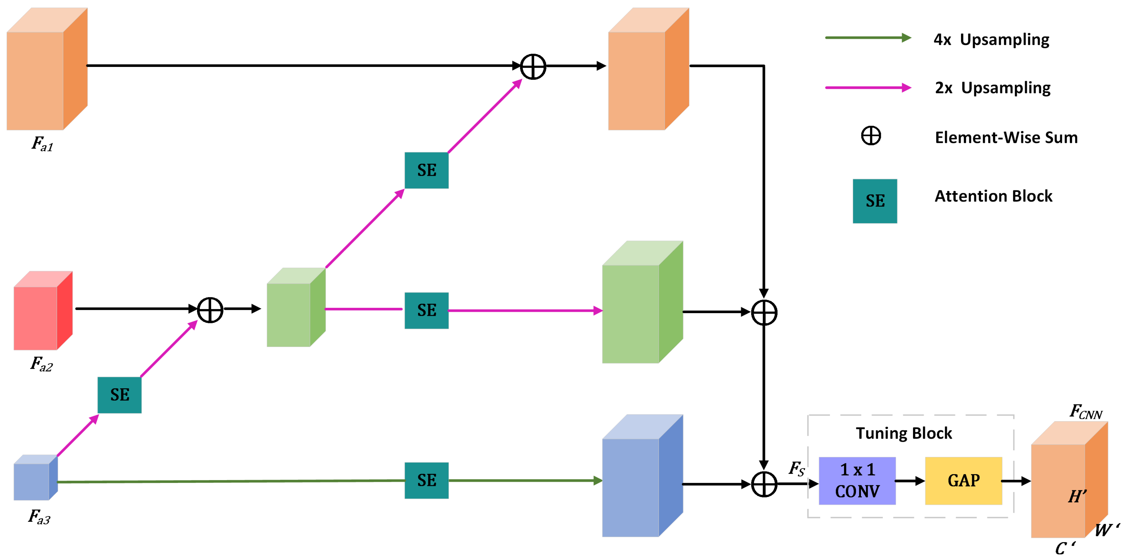
Framework of MsFFM. Features with smaller resolution are upsampled and then provided as the input to the channel attention block. The channel-optimized upsampled features are added element-wise to the adjacent features with higher resolution. Finally, we merge the all-upsampled feature map to further aggregate information, and the tuning block is adopted to refine the fused multi-scale feature. In this figure, the magenta arrow and green arrow represent the two-times upsampling operation and four-times upsampling operation, respectively, ⊕ denotes the elementwise sum operation, and is the feature map after multi-scale fusion.
Figure 4.
Framework of MsFFM. Features with smaller resolution are upsampled and then provided as the input to the channel attention block. The channel-optimized upsampled features are added element-wise to the adjacent features with higher resolution. Finally, we merge the all-upsampled feature map to further aggregate information, and the tuning block is adopted to refine the fused multi-scale feature. In this figure, the magenta arrow and green arrow represent the two-times upsampling operation and four-times upsampling operation, respectively, ⊕ denotes the elementwise sum operation, and is the feature map after multi-scale fusion.
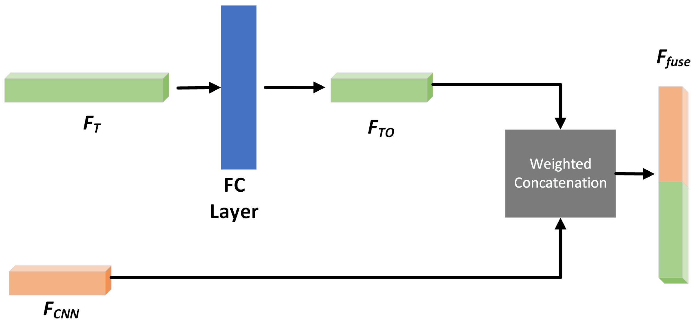
Figure 5.
The weighted concatenation method for fusing CNN features and traditional hand-crafted features . First, a fully-connected layer is adopted to ensure that the dimension of is unified with that of . Then, we set two learnable weight parameters and to reveal the importance of different features. Finally, the two features are fused by the concatenation operation.
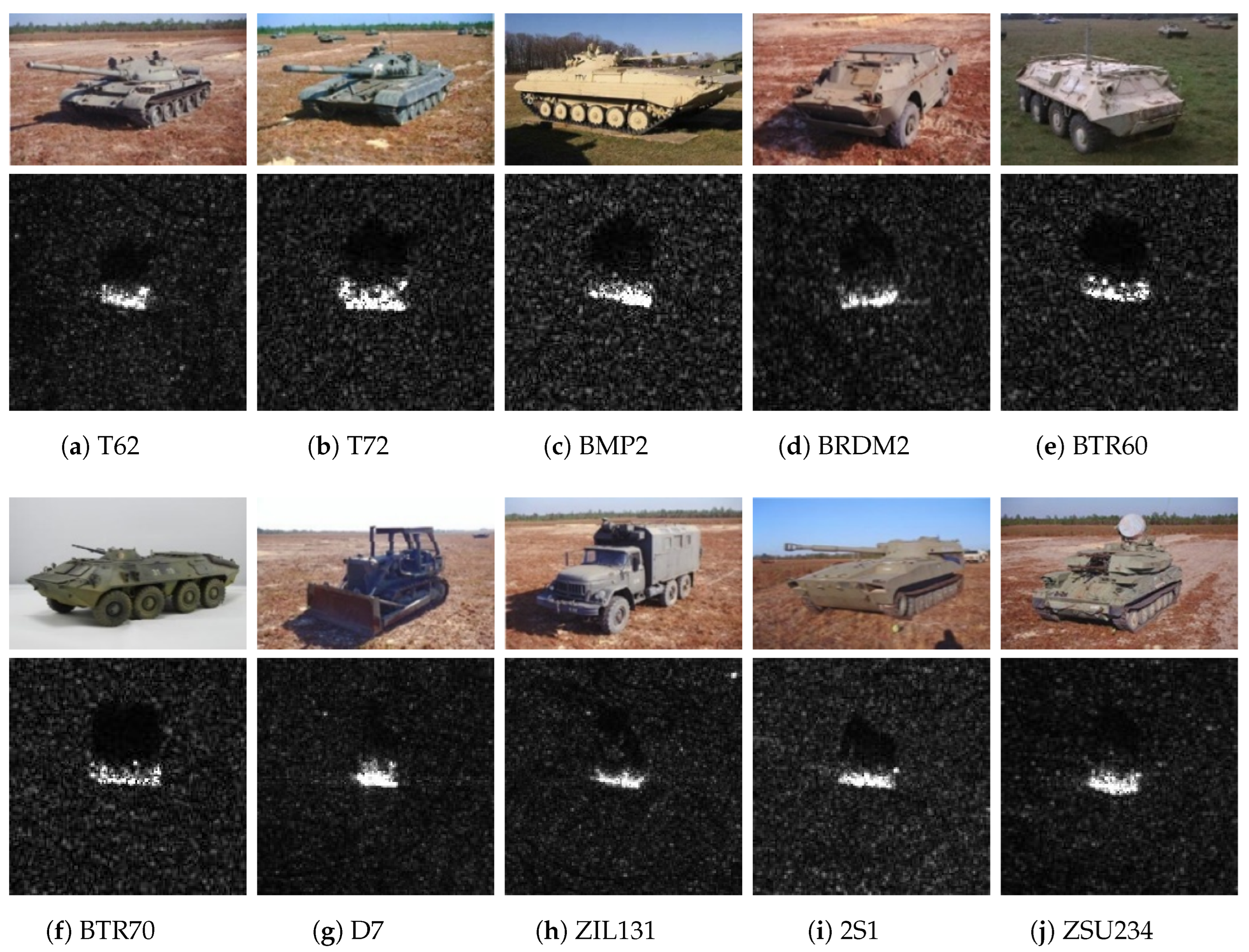
Figure 6.
The optical and SAR images in the MSTAR dataset.
Figure 6.
The optical and SAR images in the MSTAR dataset.
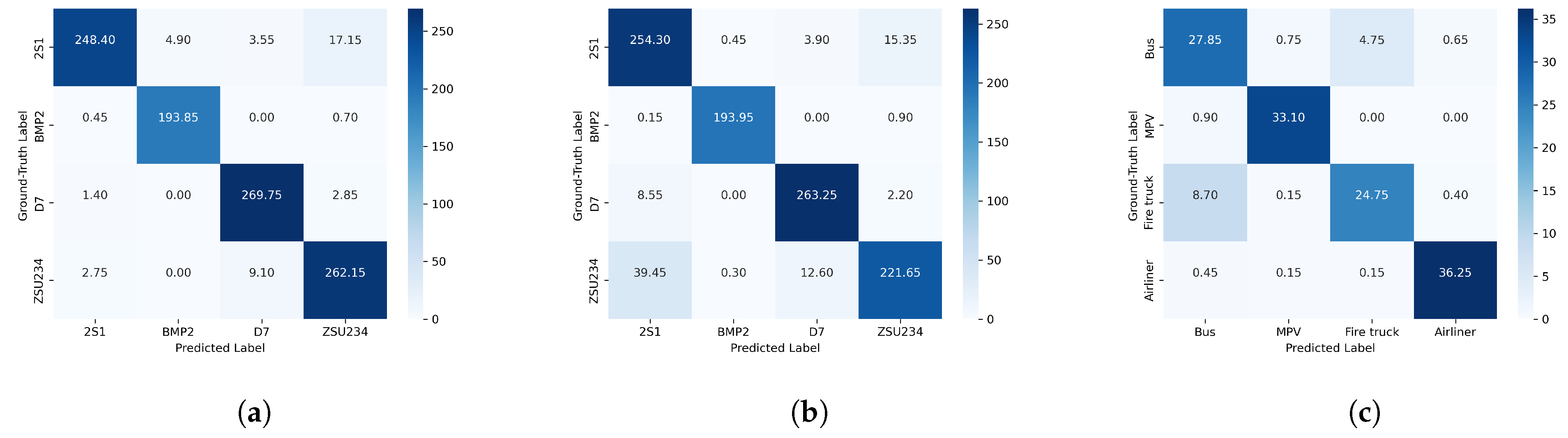
Figure 7.
The average confusion matrix of our proposed method: (a) MSTAR “4-way 5-shot” condition, (b) MSTAR “4-way 1-shot” condition, (c) VA “4-way 1-shot” condition.
Figure 7.
The average confusion matrix of our proposed method: (a) MSTAR “4-way 5-shot” condition, (b) MSTAR “4-way 1-shot” condition, (c) VA “4-way 1-shot” condition.
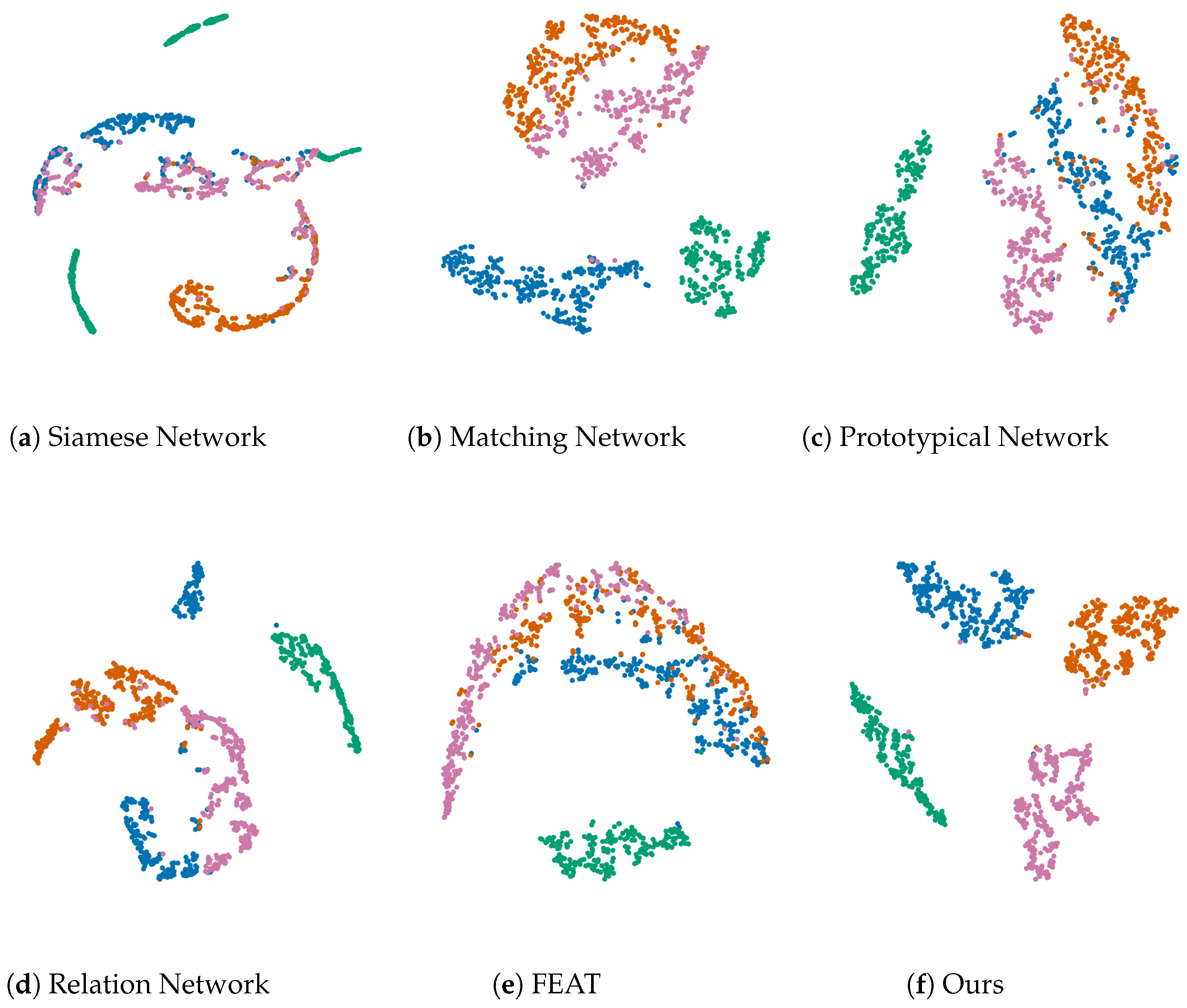
Figure 8.
The visualization results of different methods on the MSTAR dataset under the “4-way 5-shot” condition, where (a–e) denote the different comparison methods and (f) denotes our proposed method.
Figure 8.
The visualization results of different methods on the MSTAR dataset under the “4-way 5-shot” condition, where (a–e) denote the different comparison methods and (f) denotes our proposed method.
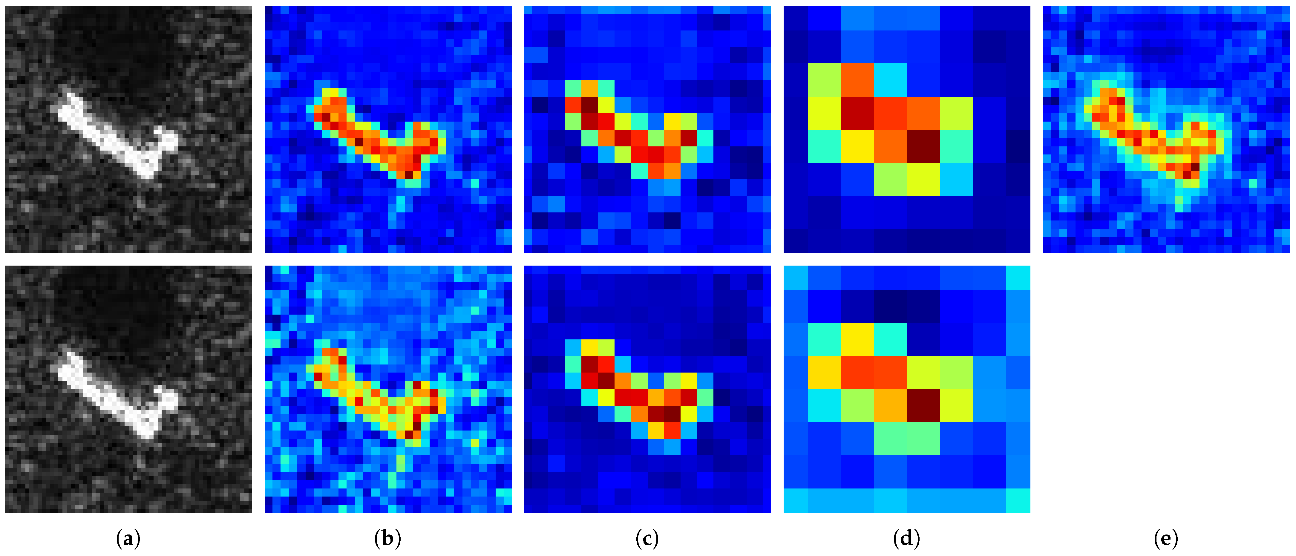
Figure 9.
The comparison of feature maps between our model and the baseline model. The first row shows the feature maps of our method and the second row the feature maps of the baseline method: (a) the input image of 2S1, (b) the feature maps on the first convolution layer, (c) the feature maps on the second convolution layer, (d) the feature maps on the third convolution layer, (e) the feature map after multi-scale feature fusion.
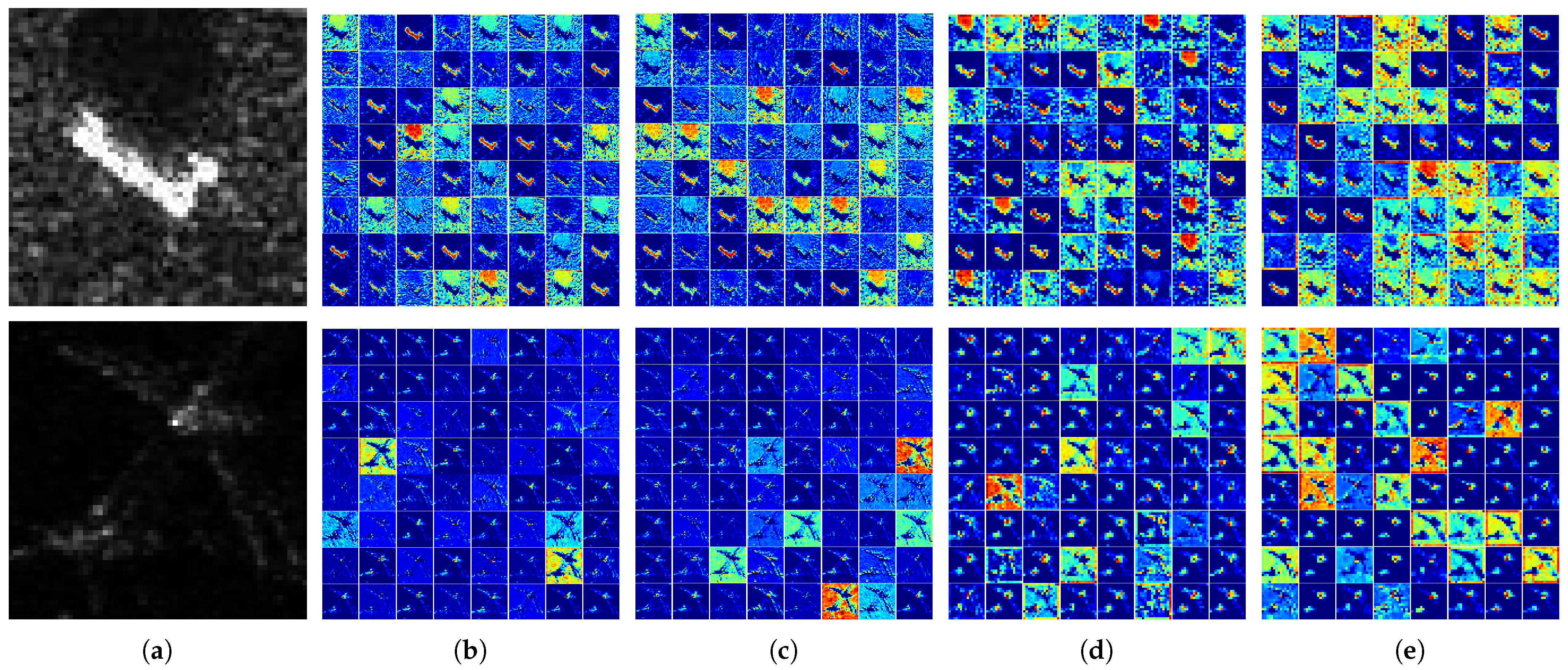
Figure 10.
Feature map comparison between baseline and our proposed model, illustrating: (a) the input image, (b) the feature maps from the first convolutional layer of our proposed model, (c) the feature maps from the first convolutional layer of the baseline model, (d) the feature maps from the second convolutional layer of our proposed model, (e) the feature maps from the first convolutional layer of the baseline model.
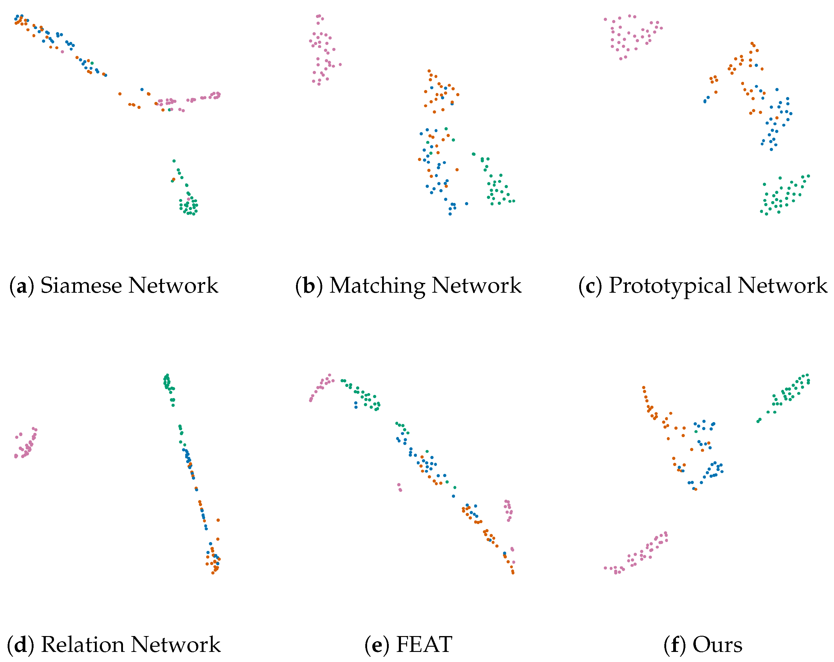
Figure 11.
The visualization result of different methods on the VA dataset under the “4-way 1-shot” condition, where (a–e) denote different comparison methods and (f) denotes our proposed method.
Figure 11.
The visualization result of different methods on the VA dataset under the “4-way 1-shot” condition, where (a–e) denote different comparison methods and (f) denotes our proposed method.
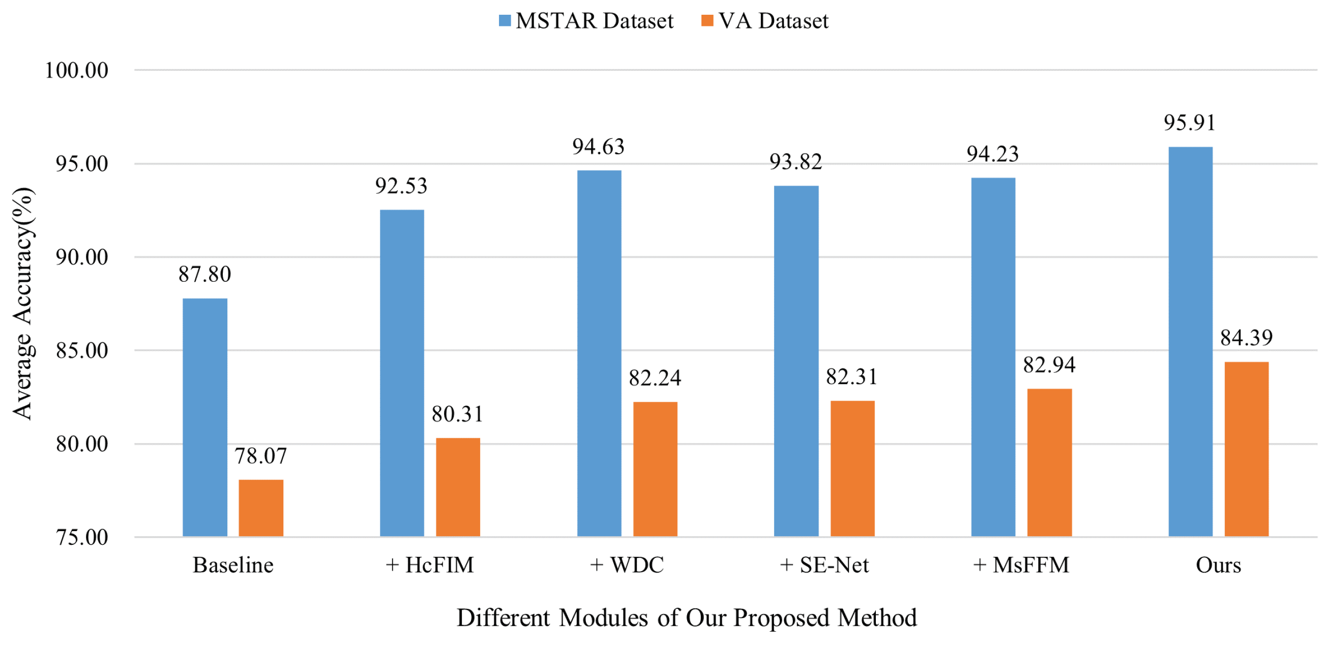
Figure 12.
Results of the ablation study on both datasets.
Figure 12.
Results of the ablation study on both datasets.
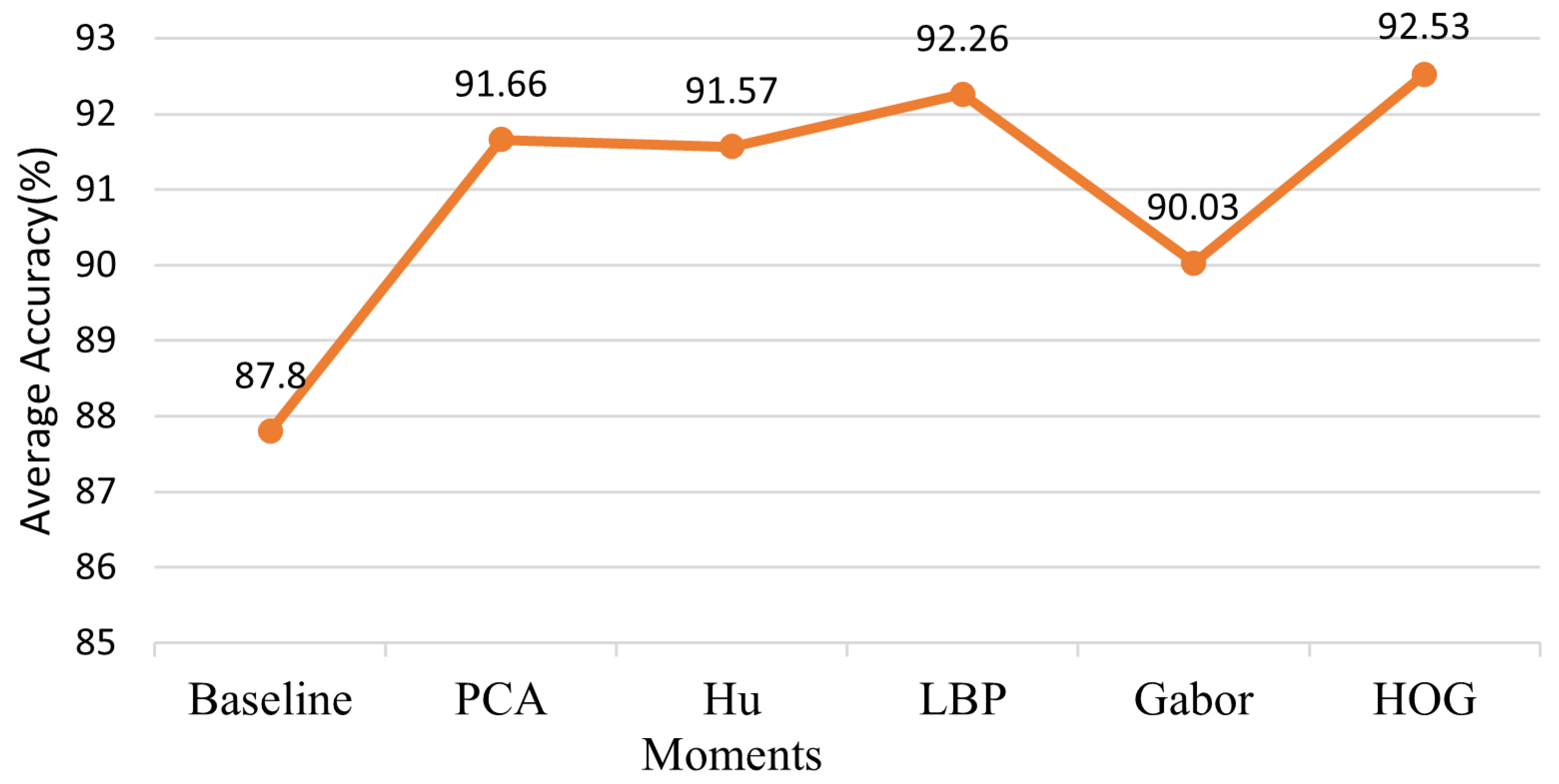
Figure 13.
The results of inserting different hand-crafted features.
Figure 13.
The results of inserting different hand-crafted features.
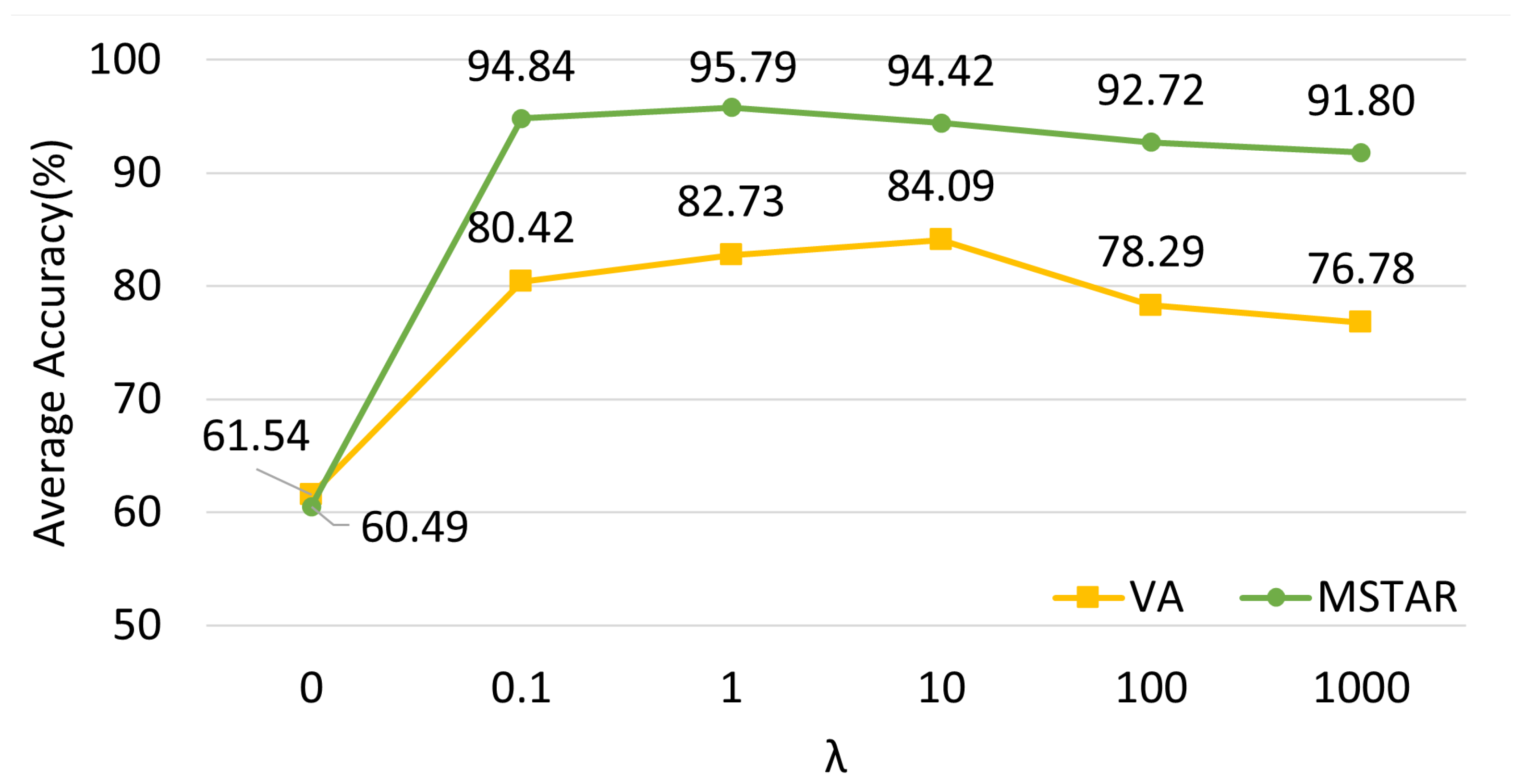
Figure 14.
The accuracy of our method under different on VA and the MSTAR datasets.
Figure 14.
The accuracy of our method under different on VA and the MSTAR datasets.
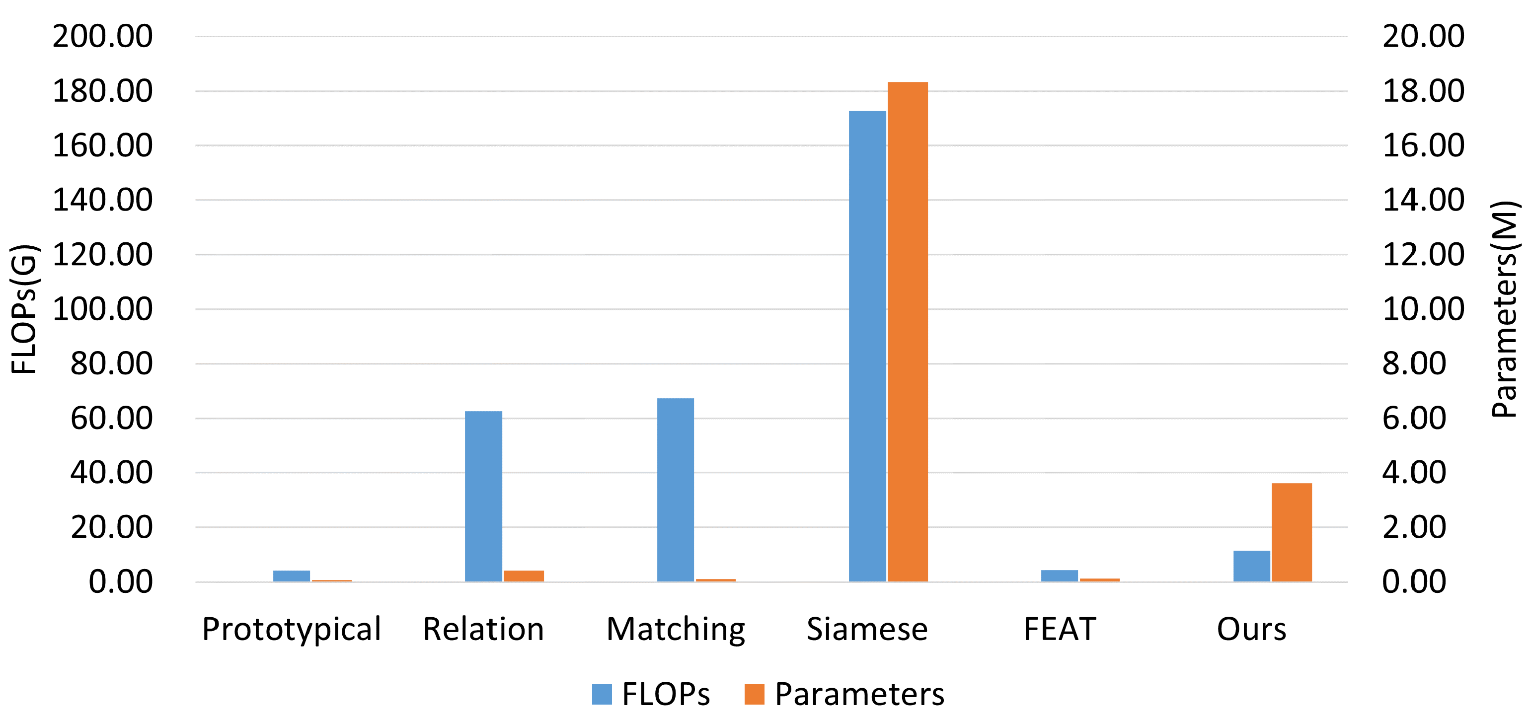
Figure 15.
Comparison of the number of parameters and FLOPs between different methods.
Figure 15.
Comparison of the number of parameters and FLOPs between different methods.
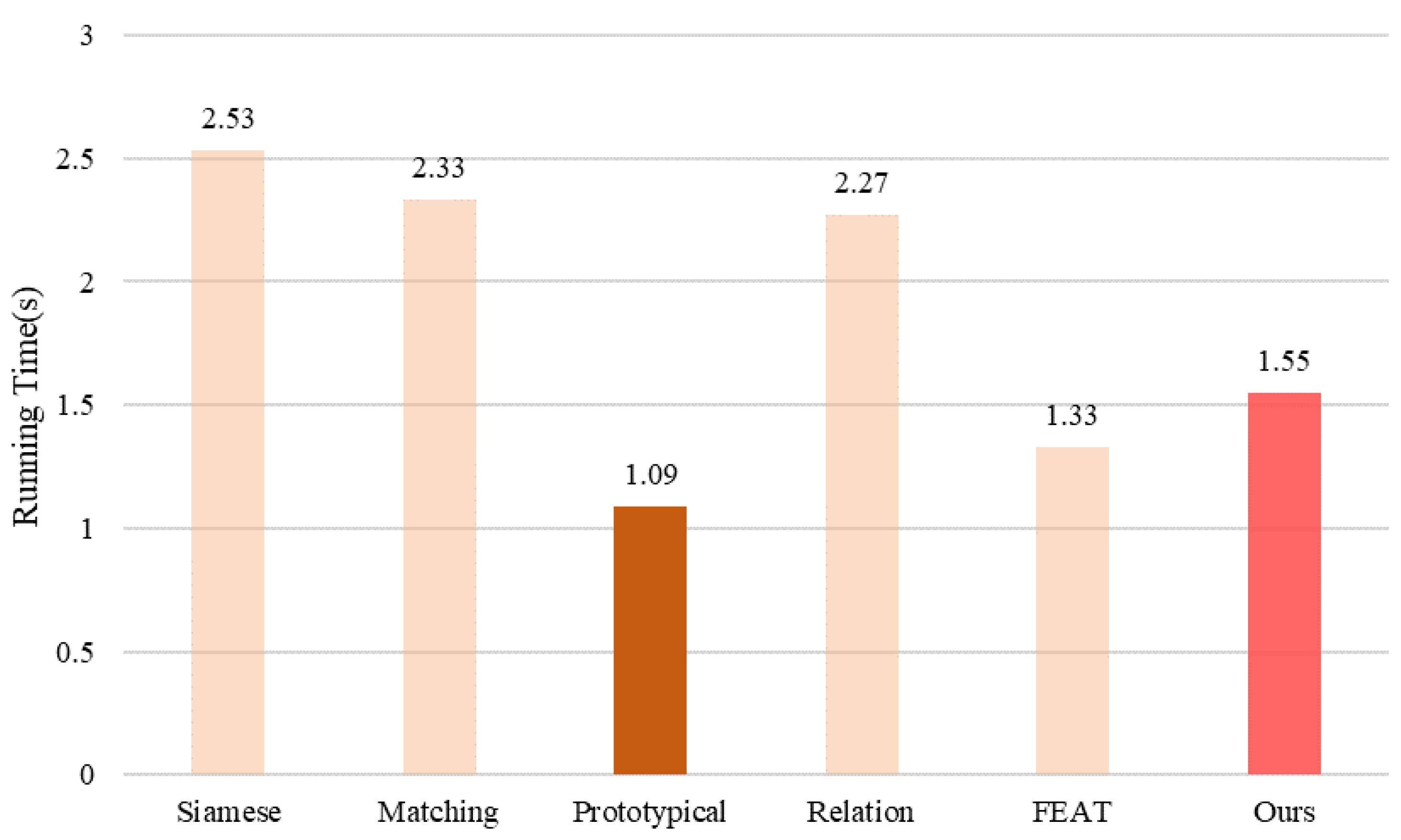
Figure 16.
The running time of different methods on the MSTAR dataset.
Figure 16.
The running time of different methods on the MSTAR dataset.
Table 1.
The number of images from each class in the MSTAR dataset.
Table 1.
The number of images from each class in the MSTAR dataset.
| Class | Depression Angle | No. | Depression Angle | No. |
|---|
| T62 | 15° | 273 | 17° | 299 |
| T72 | 15° | 196 | 17° | 232 |
| BMP2 | 15° | 195 | 17° | 233 |
| BRDM2 | 15° | 274 | 17° | 298 |
| BTR60 | 15° | 195 | 17° | 256 |
| BTR70 | 15° | 196 | 17° | 233 |
| D7 | 15° | 274 | 17° | 299 |
| ZIL131 | 15° | 274 | 17° | 299 |
| 2S1 | 15° | 274 | 17° | 299 |
| ZSU234 | 15° | 274 | 17° | 299 |
| Total | | 2425 | | 2747 |
Table 2.
The number of images in the training, support, and query sets of the MSTAR dataset.
Table 2.
The number of images in the training, support, and query sets of the MSTAR dataset.
| Training Set | Test Set |
|---|
| Support Set | Query Set |
|---|
| Class | Depression Angle | No. | Class | Depression Angle | No. | Class | Depression Angle | No. |
|---|
| T62 | 15°, 17° | 572 | BMP2 | 17° | K | BMP2 | 15° | 195 |
| T72 | 15°, 17° | 428 | D7 | 17° | K | D7 | 15° | 274 |
| BRDM2 | 15°, 17° | 572 | 2S1 | 17° | K | 2S1 | 15° | 274 |
| BTR60 | 15°, 17° | 451 | ZSU234 | 17° | K | ZSU234 | 15° | 274 |
| BTR70 | 15°, 17° | 429 | | | | | | |
| ZIL131 | 15°, 17° | 573 | | | | | | |
| Total | | 3025 | Total | 17° | | Total | 15° | 1017 |
Table 3.
The number of images from each class in the VA dataset.
Table 3.
The number of images from each class in the VA dataset.
| Class | Car | Truck | Bus | MPV | Fire Truck | Airliner | Helicopter | Total |
|---|
| No. | 35 | 35 | 35 | 35 | 35 | 38 | 70 | 283 |
Table 4.
The number of images in the training, support and query sets of the VA dataset.
Table 4.
The number of images in the training, support and query sets of the VA dataset.
| Training Set | Test Set |
|---|
| Support Set | Query Set |
|---|
| Class | No. | Class | No. | Class | No. |
|---|
| Car | 35 | Bus | 1 | Bus | 34 |
| Truck | 35 | MPV | 1 | MPV | 34 |
| Helicopter | 70 | Fire Truck | 1 | Fire Truck | 34 |
| | | Airliner | 1 | Airliner | 37 |
| Total | 140 | Total | 4 | Total | 139 |
Table 5.
“4-way 5-shot” recognition performance of different methods on the MSTAR dataset.
Table 5.
“4-way 5-shot” recognition performance of different methods on the MSTAR dataset.
| Methods | Min Accuracy (%) | Max Accuracy (%) | Average Accuracy (%) |
|---|
| Siamese | 63.42 | 83.48 | 72.49 ± 5.46 |
| FEAT | 70.50 | 89.97 | 81.23 ± 4.08 |
| Prototypical | 75.42 | 92.14 | 87.80 ± 4.35 |
| Matching | 80.53 | 94.11 | 91.58 ± 3.01 |
| Relation | 68.93 | 94.30 | 80.85 ± 5.84 |
| Ours | 93.31 | 99.21 | 95.79 ± 1.27 |
Table 6.
“4-way 1-shot” recognition performance of different methods on the MSTAR dataset.
Table 6.
“4-way 1-shot” recognition performance of different methods on the MSTAR dataset.
| Methods | Min Accuracy (%) | Max Accuracy (%) | Average Accuracy (%) |
|---|
| Siamese | 57.72 | 77.09 | 68.07 ± 5.12 |
| FEAT | 70.50 | 89.97 | 71.04 ± 8.23 |
| Prototypical | 56.44 | 91.35 | 74.65 ± 8.43 |
| Matching | 60.87 | 86.43 | 79.59 ± 7.25 |
| Relation | 55.95 | 83.38 | 69.19 ± 8.84 |
| Ours | 85.94 | 96.85 | 91.76 ± 3.40 |
Table 7.
“4-way 1-shot” recognition performance of different methods on the VA dataset.
Table 7.
“4-way 1-shot” recognition performance of different methods on the VA dataset.
| Methods | Min Accuracy (%) | Max Accuracy (%) | Average Accuracy (%) |
|---|
| FEAT | 58.74 | 82.93 | 73.03 ± 6.36 |
| Siamese | 53.15 | 76.42 | 69.94 ± 5.86 |
| Prototypical | 68.53 | 82.12 | 78.07 ± 4.14 |
| Matching | 60.84 | 84.56 | 73.46 ± 6.24 |
| Relation | 58.04 | 87.80 | 77.33 ± 6.77 |
| Ours | 76.92 | 90.21 | 85.28 ± 3.82 |
Table 8.
The results of further ablation study on both datasets.
Table 8.
The results of further ablation study on both datasets.
| Baseline | MsFFM | HCFIM | WDC + New Loss | SE-Net | Average Accuracy (%) |
|---|
| MSTAR Dataset | VA Dataset |
|---|
| √ | | | | | 87.80 | 78.07 |
| | √ | | | | 94.23 | 82.94 |
| | √ | √ | | | 94.35 | 83.00 |
| | √ | √ | √ | | 95.18 | 84.23 |
| | √ | √ | √ | √ | 95.79 | 84.39 |
Table 9.
The results of different concatenating schemes for hand-crafted features and CNN features.
Table 9.
The results of different concatenating schemes for hand-crafted features and CNN features.
| Baseline | Concatenation | Learnable Coefficients | Feature Embedding | Average Accuracy (%) |
|---|
| √ | | | | 87.80 |
| | √ | | | 91.48 |
| | √ | √ | | 92.06 |
| | √ | | √ | 91.86 |
| | √ | √ | √ | 92.53 |


