Fine-Grained Classification of Optical Remote Sensing Ship Images Based on Deep Convolution Neural Network

Abstract

Marine activities occupy an important position in human society. The accurate classification of ships is an effective monitoring method. However, traditional image classification has the problem of low classification accuracy, and the corresponding ship dataset also has the problem of long-tail distribution. Aimed at solving these problems, this paper proposes a fine-grained classification method of optical remote sensing ship images based on deep convolution neural network. We use three-level images to extract three-level features for classification. The first-level image is the original image as an auxiliary. The specific position of the ship in the original image is located by the gradient-weighted class activation mapping. The target-level image as the second-level image is obtained by threshold processing the class activation map. The third-level image is the midship position image extracted from the target image. Then we add self-calibrated convolutions to the feature extraction network to enrich the output features. Finally, the class imbalance is solved by reweighting the class-balanced loss function. Experimental results show that we can achieve accuracies of 92.81%, 93.54% and 93.97%, respectively, after applying the proposed method on different datasets. Compared with other classification methods, this method has a higher accuracy in optical aerospace remote sensing ship classification.

1. Introduction

With the rapid development of optical remote sensing technology, this technology has been widely used in resource exploration, disaster inspection, ocean conservation, military command, and so on. As an important target of maritime activities, a highly accurate classification of ships is of great significance. Optical remote sensing ship image classification [1] has garnered considerable attention from all areas and plays an important role in combating smuggling and military command. A highly qualified classification algorithm of maritime targets can efficiently distinguish oil tankers from warships, enabling authorities to take appropriate action quickly. Due to the great significance of protecting territorial sea rights and maintaining regional stability, improving the method for remote sensing ship images classification is urgent.

Traditional remote sensing ship image classification depends on many various factors. Early classification methods relied on global features. The shape and texture features used in these methods [2,3] belong to low-level global features. But global features can only be classified simply. Other scholars have found that local features are more discriminative. Leng et al. [4] proposed a comb feature to analyze different categories of ships in high-resolution remote sensing. However, feature-based methods generally have the problems of low accuracy and slow speed. In addition, the Bayesian network [5] and the support vector machine (SVM) [6] are also used to identify remote sensing ships. However, SVM is designed for binary classification and its performance will decrease when doing multi-classification. Recently, the image classification network based on deep learning has achieved good results [7]. A two-branch convolutional neural network (CNN) method [8] is used to extract features for remote sensing ship classification. This network benefits from an advanced performance based on 2-dimensional discrete fractional Fourier-transform (2D-DFrFT). Liu et al. [9] used the improved InceptionV3 and center loss convolution neural network to classify ships in remote sensing images. These methods have achieved good results in remote sensing ship classification for a small number of ship categories. However, traditional remote sensing ship classification methods have difficulty in dealing with more categories and more detailed subcategories. At present, fine-grained ship classification methods have achieved better results in classifying sub-category ship types [10].

According to different classification levels, image classification can be divided into coarse-grained classification and fine-grained classification. Coarse-grained classification is used to classify basic categories. Conversely, fine-grained classification is used to distinguish different subcategories under the same broad category. The different ship categories classified in this paper belong to the same broad category and there are subtle differences between different subcategories. As shown in Figure 1a, the ferry boat and the ocean liner are similar in appearance. They are only partially different in deck superstructure. At the same time, ships have large intra-class differences. As shown in Figure 1b, the superstructure may be on the bow and stern of the container ship. Moreover, different ships also have obvious differences in color and other aspects.

At present, the requirements for ship classification are more detailed, and various fine-grained classification methods are also applied in this field [11]. Zhang et al. [1] proposed an attribute-guided multi-level enhanced feature representation network (AMEFRN), which used multi-level enhanced visual features for fine-grained ship image classification. This method has high accuracy, but it cannot solve the problem of class imbalance. Hu and Qi [12] proposed a weakly supervised data attention network (WSDAN), which combines weakly supervised learning and data augmentation to identify different objects with similar features.

The existing fine-grained classification methods for remote sensing ships have problems in the following three aspects.

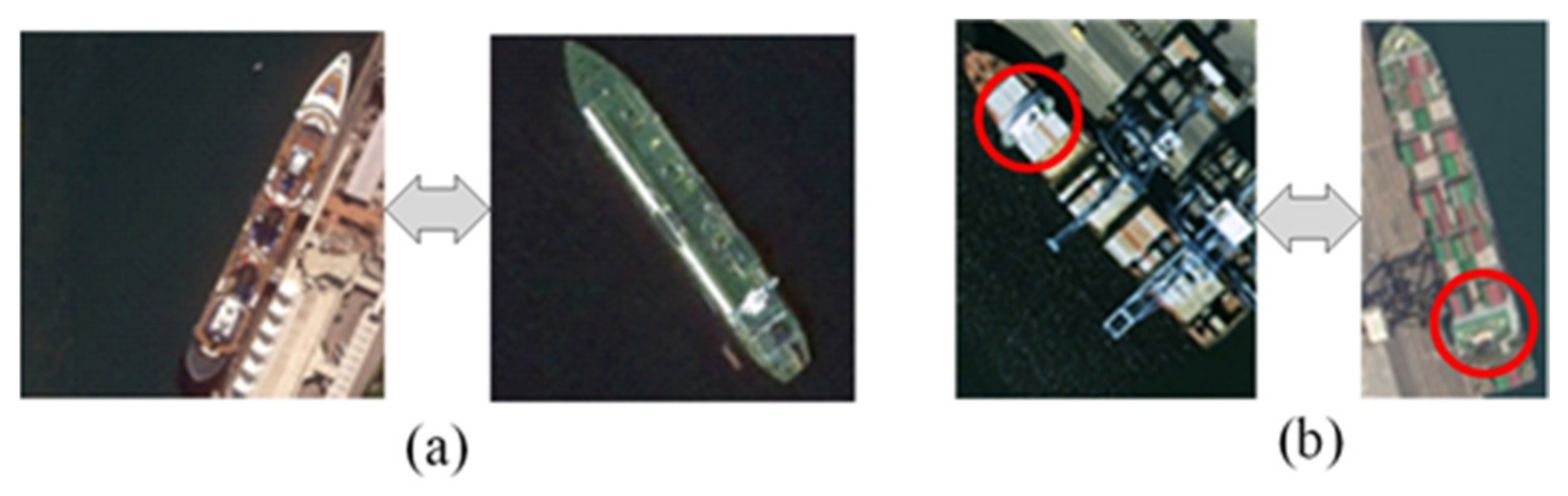
• Intra-class difference. Ships of the same kind differ in the layout of their deck superstructure.
• Inter-class similarity. Different categories of ships may also have some similar features.
• Long-tailed distribution. The number of each category in the dataset is seriously unbalanced.

In response to the above problems, this paper proposes a fine-grained classification method for the remote sensing of ships. The main contributions of this paper are as follows.

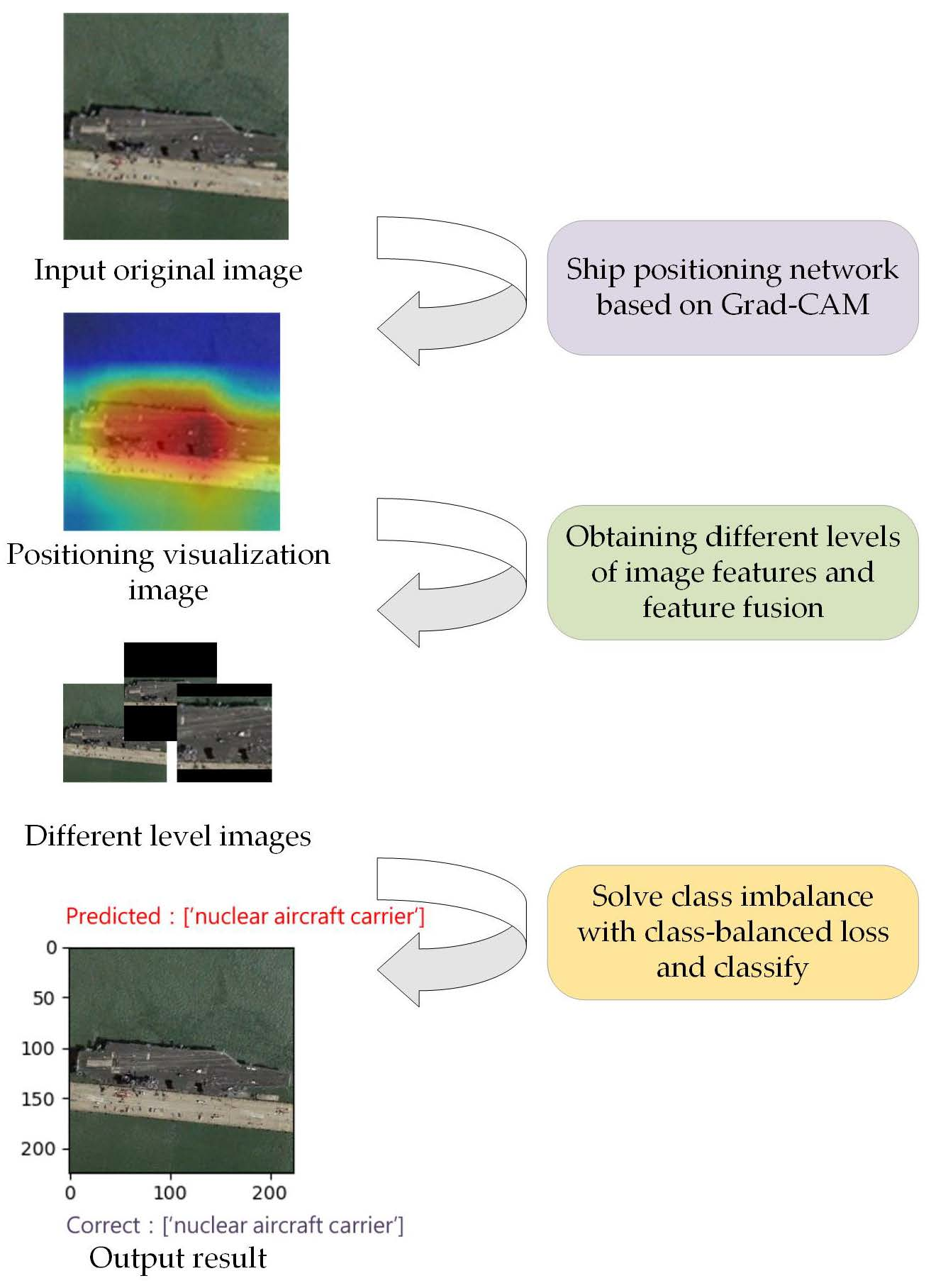
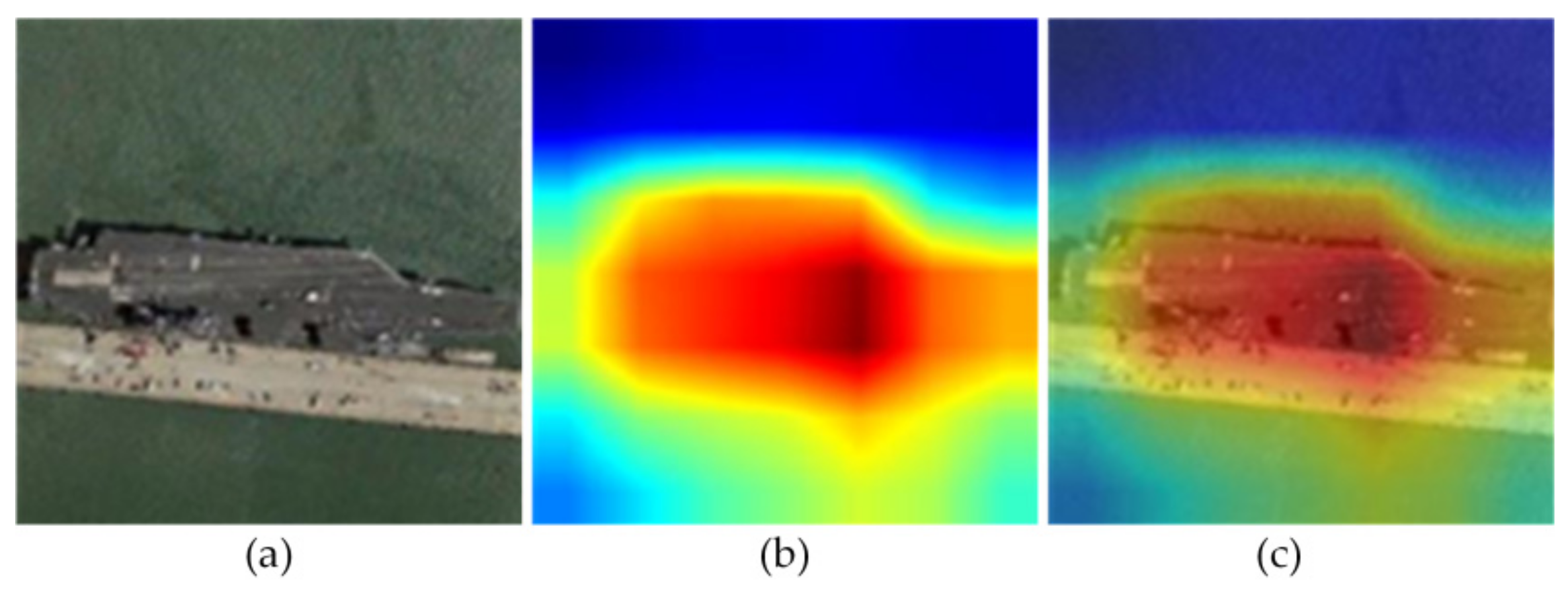
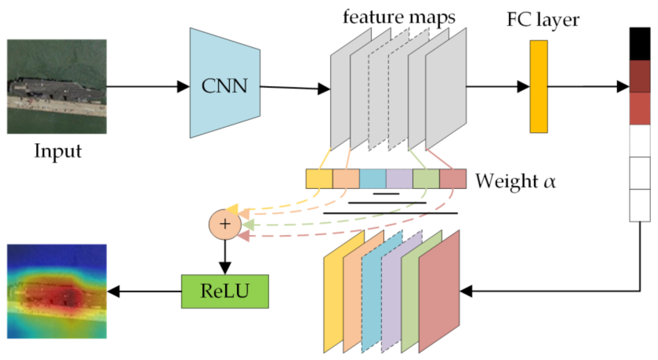
• Gradient-weighted class activation mapping (Grad-CAM) is used to locate the ship position from the images and obtain the midship area with rich information. Then, the categories of the ship are finely recognized by fusing the global and local features of the image.
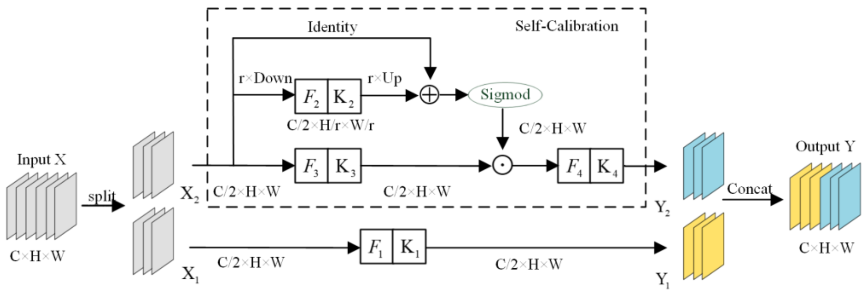
• By adding self-calibrated convolutions (SC-conv) [13] to the classification network, different contextual information is collected to expand the field of vision and enrich the output features.
• By introducing the class-balanced loss (CB loss), the samples are re-weighted to solve the long-tail distribution problem of the remote sensing ship image dataset.

The rest of this paper is organized as follows. Section 2 reviews the related work. Section 3 is the ship category recognition model. Section 4 introduces the experiments and discussion while Section 5 introduces the research conclusion.

2. Related Work

Fine-grained image classification can be divided into location-recognition methods, network integration methods, and convolution feature high-order coding methods. The methods based on location recognition need to find the discriminative part. Then perform feature extraction and classification. These methods can be divided into strong supervision and weak supervision. The strong supervision methods require not only category labels but also component labels and key position boxes. Region-based CNN (R–CNN) [14] was proposed to learn the global and local features of objects. Branson et al. [15] proposed to perform pose alignment operations on the part-level image blocks for classification. However, the above strong supervision fine-grained image classification methods have many disadvantages. The labeling position and boundary box consume a lot of manpower and material resources.

The weak supervision methods do not need component labels and only rely on category labels to complete the training. The two-level attention algorithm is used to classify birds by the object level and part level, respectively [16]. MA-CNN clustered channels with similar response regions to get the attention part [17]. DFL-CNN used the 1 × 1 × C convolution kernel to detect discriminant regions and then adopted an asymmetric multi-branch network structure [18]. This method uses both local and global information. DCL divides the input image into local regions and shuffles them through the region confusion mechanism [19]. Then, it modeled the semantic correlation between local regions. The HBP network is used to capture the feature relationship between layers [20]. Based on bilinear pooling, LRBP network used low-rank approximation to the covariance matrix to further reduce the computational complexity [21]. However, bilinear pooling has the problem of the feature dimension being too high after fusion. RA-CNN recursively learns the discriminative area attention and the area-based feature representation in a mutually reinforcing way [22]. It inputted area maps of different scales and learns features on different scales to predict categories. However, the remote sensing ship image is limited by the features of the ship’s rigid target and the disadvantages of optical remote sensing imaging. There are some problems in the images, such as inter-class similarity. Thus, it is difficult to achieve high accuracy in optical remote sensing image classification.

Locating the objects in the image can effectively reduce the background interference and improve the performance of images classification. Zhou et al. [23] proposed the class activation mapping (CAM). It multiplied the output of each layer by the weight of the corresponding classification of that layer and weighted the results. Then the class activation mapping of the target is obtained. The judgment feature position with certain discrimination ability is obtained by this way. However, this method has some limitations. It modified the fully connected (FC) into the convolutional layer and the maximum pooling layer. Consequently, the improved version of CAM, Grad-CAM [24] used the global average of the gradient to calculate the weight and the calculated weight is equivalent to the CAM weight. Furthermore, it avoided the modification of the original network structure. This paper uses Grad-CAM to locate the ship. On this basis, the ship positioning image and key part image are cut out. Then, three-level image feature input is performed to enhance the performance of the classification network.

Long-tail distribution is a common problem in the image classification dataset. This problem is particularly serious in remote sensing images of ships. On the one hand, there are many optical remote sensing satellites in orbit, but few are open to the public. Therefore, the amount of data that can be collected is limited. On the other hand, the number of ships of various types is also quite different. There are more than 24,000 bulk carriers engaged in ocean-going voyages, while there are only 22 active aircraft carriers. Since aircraft carriers are an extremely important class of combat ships, they cannot be excluded from the dataset. This creates an extremely unbalanced data distribution. The classification algorithm based on deep learning has a poor learning effect on tail categories. At present, there are various optimization methods to solve the recognition problem under the long-tail distribution, including re-sampling [25], re-weighting [26], and transfer learning [27]. Re-sampling includes undersampling of the head category samples and oversampling of the tail. However, oversampling might be overfit in the tail category. Moreover, undersampling may lose too much head category information and lead to under-fitting. Transfer learning transfers the head category feature knowledge learned by the model to the tail category. The disadvantage is that it usually needs to design additional complex modules. Re-weighting adjusts the proportion of each category loss in the total loss to alleviate the imbalance of the gradient proportion caused by the long-tail distribution. Cui et al. [26] proposed the concept of the effective number of samples. They realized the weighting process by adding a class-balance weighting item that is inversely proportional to the effective number of samples in the loss. The reciprocal of the effective number of samples N used for CB loss is more accurate when weighting the loss. Long-tailed distributions in datasets can be better addressed using the CB loss.

3. Materials and Methods

On one hand, global features usually play a significant role in the feature extraction of ship images. Global features including the aspect ratio, color features, and appearance features of the ships. Each category of ship has its own global features.

On the other hand, remote sensing images of ships have special properties. As artificial objects, ships are different from natural objects such as birds and dogs. Thus, there is no clear location for its parts. Therefore, we choose the midship as the key part of the ships. In this position, the features of ships within the same category tend to be similar while the characteristics of ships of different categories are significantly different.

As shown in Figure 2a,b, different categories of container ships are loaded with containers in the midship. The midship of the nuclear-powered aircraft carrier is the apron and landing runway as shown in Figure 2c. It can be seen from Figure 2d–f that there are obvious differences in the midships of various categories of warships. The midship of the guided missile frigate is covered with radar masts, chimneys, and the front half of the hangar. The guided missile destroyer mainly has the chimney in this place. The guided missile cruiser also has a helicopter deck in the midship.

The complete process of the fine-grained remote sensing ship classification network algorithm based on object positioning is shown in Algorithm 1. First, the class activation map of the original image is extracted by Grad-CAM. Then, threshold segmentation is performed on the class activation map to generate a mask image. Next, the mask image is used to cover the original image to obtain the location map. The key part image and the target-level image are extracted by cutting the positioning maps. The feature vector of the three-level image is obtained through CNN. The SC-conv is added to the feature extraction network of the three images to improve the richness of the output features. Finally, the feature vectors are fused, and the CB loss is used to reduce the error caused by class imbalance.

Algorithm 1. The recognition process of fine-grained optical remote sensing ships.

Input: The original image $I(x,y)$. 1     Obtaining class activation maps by Grad-CAM. 2     for each original image in the dataset do 3     Get the ship target-level image $t(x,y)$ and key part image are obtained by threshold segmentation; 4      Take SC-conv to obtain the features of the three-level input images, respectively; 5     Fusion of feature vectors; 6     Using CB loss to reduce the error caused by the long-tailed distribution of the dataset;  Output: Classification results.

The model structure of fine-grained remote sensing ship classification network in this paper is shown in Figure 3. It is divided into two parts. Figure 3a is the ship positioning network and Figure 3b shows the extraction of two-stage image. Figure 3c,d is the SC-conv network and CB loss, respectively.

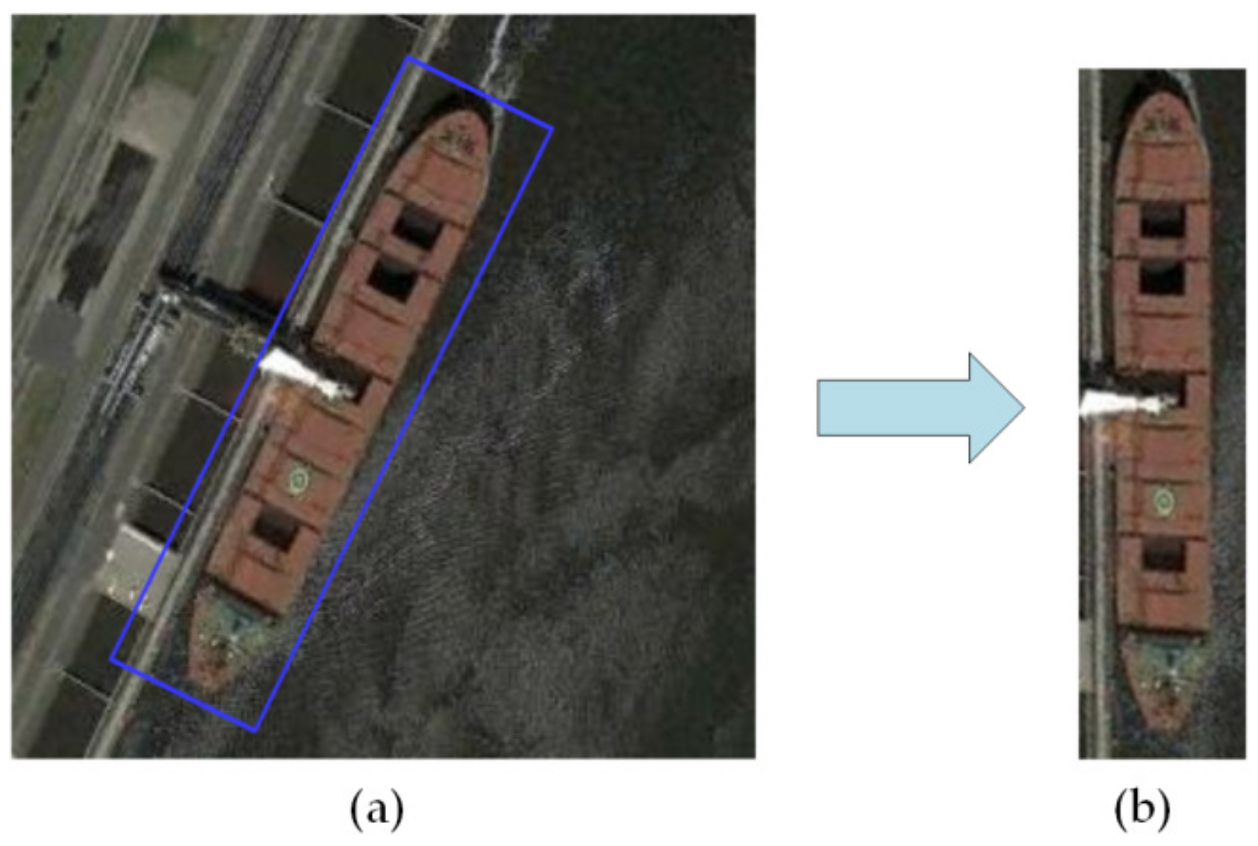
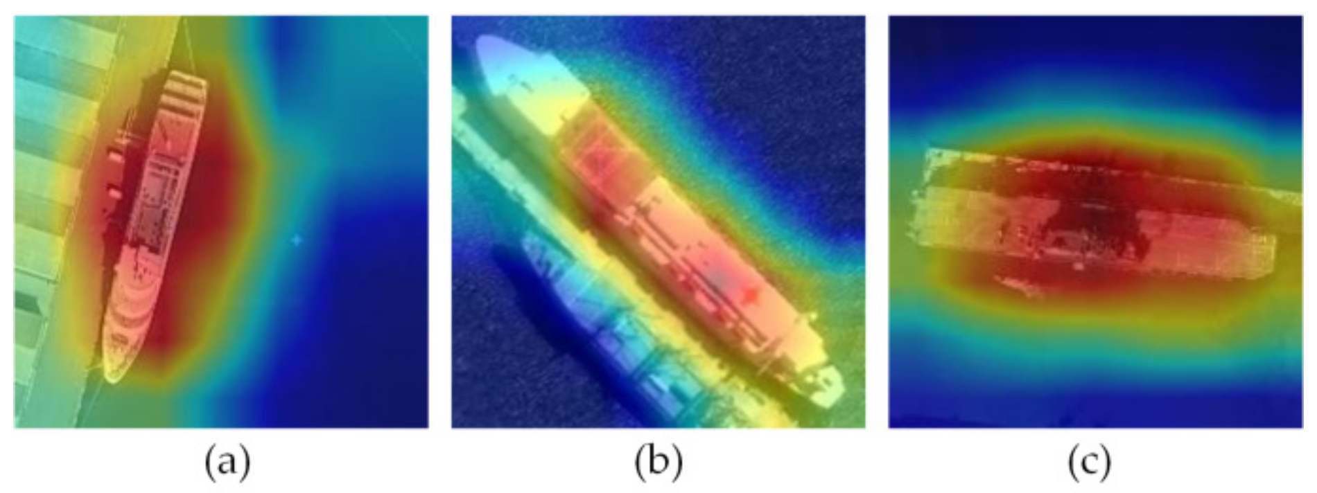
3.1. Target Location Based on Grad-CAM

The complex and diverse sea surface conditions have a serious impact on image classification. In order to better identify the type of ships, the useless background information should be excluded first. So, determine the position of the ship in the image and crop accordingly. The cropped image is fed into the next step of the network. This paper uses class activation mapping for localization.

For a deep CNN, its last convolutional layer contains the most abundant spatial and semantic information after multiple convolutions and pooling. CAM can use this information effectively [23].

Grad-CAM adopts another method, which uses the global average of the gradient to calculate the weight. This avoids modifying the original network model structure [24]. Grad-CAM uses the heat map to represent the significant areas, as shown in Figure 4. Figure 4a is the input original image, and Figure 4b is the output heat map. The significance becomes strong from the blue area to the red area. Figure 4c is the image after the two are superimposed. It can be seen that the position of the ship is consistent with the red area.

The specific process is shown in Figure 5. We calculate the feature map obtained after the last convolution. The last layer contains $n$ feature maps, and each feature map mainly extracts some features related to a certain category. The gradients are set to zero for all classes except the desired class. We use this signal and the resulting convolution feature maps to calculate the Grad-CAM heat map.

Grad-CAM finds the gradient of the last layer of convolutional layer and the average value of the gradient of each feature map is used as the weight of the feature map. Define the weight of feature map $k$ to category $c$ in Grad-CAM as ${\alpha }_k^c$. It uses the global average pooling (GAP) to obtain ${\alpha }_k^c$. The weight is calculated by:

$${\alpha }_k^c=\frac{1}{Z}{\displaystyle \sum }_i{\displaystyle \sum }_j\frac{\partial y^c}{\partial A_{ij}^k}$$

(1)

where, $Z$ is the number of pixels of the feature map, $y^c$ is the score gradient corresponding to category $c$, $A_{ij}^k$ represents the pixel value at position $\left(i,j\right)$ in the feature map $k$. After obtaining the weight of the category to all the feature maps, calculate the weighted sum to get the class activation map of category $c$. As shown in Equation (2):

$$L_{Grad-CAM}^c=ReLU\left({\displaystyle \sum }_k{\alpha }_k^c{A}^k\right)$$

(2)

where ReLU is the activation function, which is used to remove negative values. The resulting class activation map will be sent to Section 3.2. Extraction of two-stage image.

Perform threshold segmentation on the class activation map extracted in Section 3.1 to cover the background part. The position of the ship to be located is obtained by threshold segmentation. The ship image without interference is obtained by superposing the binary image with the original image. The specific operation is as follows:

In the first step of the mask filter, the object significance region is determined according to the threshold processing in Equation (3). The regions larger than the set threshold are set to 1 and the regions less than the set threshold are set to 0.

$$p\left(x,\mathrm{y}\right)=\left\{\begin{array}{c}1,M\left(x,y\right)\ge ts\\ 0,M\left(x,y\right)<ts\end{array}\right.$$

(3)

where $p\left(x,y\right)$ represents the pixel value of the mask at position $\left(x,y\right)$, and $M\left(x,y\right)$ is the class activation map. Then obtain the saliency area of the object and the part of pixel $p\left(x,y\right)=1$.

We binarize the Grad-CAM with a threshold of 20% of the max intensity. When the threshold is too large, part of the target will be obscured, and if the threshold is too small, more invalid background information will be retained. This operation will generate connected pixel segments. Then, based on the original image $I\left(x,y\right)$, the target image $t\left(x,y\right)$ is obtained by using the mask $p\left(x,y\right)$ of the significance region, as below:

$$t\left(x,y\right)=I\left(x,y\right)\cdot p\left(x,y\right)$$

(4)

To better identify remotely-sensed ship images, it is necessary to eliminate the interference of background information to the greatest extent. The specific position of the ship needs to be determined in the process of fine-grained network recognition. Subsequently, the images are cropped and enlarged.

Perform edge extraction on the $t\left(x,y\right)$ obtained in the previous section to detect the contour. Then find the minimum area rectangle of the ship. Next get the center position, width, height, and rotation angle of the minimum area rectangle to perform the affine mapping. Then the original image is cropped according to the bounding to obtain the target-level image, as shown in Figure 6.

The process of affine transformation is as follows. The vector space undergoes a linear transformation followed by a translation. Transform it into another vector space in geometry. In the case of finite dimensions, each affine transformation can be given by a matrix $A$ and a vector $t$. The affine transformation equation is shown in Equation (5).

$$\beta =A\alpha +t$$

(5)

The affine transformation corresponds to the multiplication of a matrix and a vector. Correspondingly, the composition of the affine transformation requires adding an extra row to the bottom of the matrix. This rightmost side of this row is 1 and the others are 0. Then, a number 1 is added to the bottom of the column vector. The affine transformation between two-dimensional coordinates can be expressed by Equation (6).

$$\left[\begin{array}{c}{x}^{\prime }\\ y^{\prime }\\ 1\end{array}\right]=\left[\begin{array}{ccc}{a}_1& a_2& t_x\\ a_3& a_4& t_y\\ 0& 0& 1\end{array}\right]\left[\begin{array}{c}x\\ y\\ 1\end{array}\right]$$

(6)

where $\left(t_x,t_y\right)$ is the amount of translation of the image and $a_i$ represents zoom, rotation, shearing, etc. Calculate the parameters $t_x$, $t_y$, $a_i$, etc. to get the affine transformation relationship of the image.

The next step is to take the long side of the target image as the benchmark. The midship position image in the 1/3 in the middle of the long side is used as the key part image.

3.2. Self-Calibrated Convolutions

In the process of ship image classification, establishing long-range dependencies is of great help for accurate feature extraction. Self-calibrated convolutional networks can expand the field of view of each convolutional layer, thereby enriching the output features. Unlike standard convolution, SC-conv can adaptively establish long-range spatial and channel relationships through self-calibration operations [13].

As shown in Figure 7, the input $\mathrm{X}$ is evenly divided into two parts ${\mathrm{X}}_1$ and ${\mathrm{X}}_2$ to collect different contextual information. For ${\mathrm{X}}_2$, we use ${\mathrm{K}}_2$, ${\mathrm{K}}_3$ and ${\mathrm{K}}_4$ to perform self-calibration to get ${\mathrm{Y}}_2$. To preserve the original spatial context information, a simple convolution operation is performed on ${\mathrm{X}}_1$. Then we concatenate ${\mathrm{Y}}_1$ and ${\mathrm{Y}}_2$ to get the output $\mathrm{Y}$. The shape of each filter is $\left(C/2,C/2,k_h,k_w\right)$.

A simple convolution operation is performed in the first branch to ensure that the original context information is retained. The calculation process is shown in Equation (7).

$${\mathrm{Y}}_1={\mathcal{F}}_1\left({\mathrm{X}}_1\right)={\mathrm{X}}_1\ast {\mathrm{K}}_1$$

(7)

Given the input ${\mathrm{X}}_2$, we adopt the average pooling with filter size r × r and stride r as follows:

$$\mathrm{T}={\mathrm{AvgPool}}_r\left({\mathrm{X}}_2\right)$$

(8)

The output after up sampling is:

$${\mathrm{X}}_2^{’}=\mathrm{Up}\left({\mathcal{F}}_2\left(\mathrm{T}\right)\right)=\mathrm{Up}\left(\mathrm{T}\ast {\mathrm{K}}_2\right)$$

(9)

where $\mathcal{F}$ stands for the filter, $\ast$ stands for convolution, $\mathrm{Up}\left(\cdot \right)$ is a bilinear interpolation operator. The formula for the calibration operation is:

$${\mathrm{Y}}_2^{’}={\mathcal{F}}_3\left({\mathrm{X}}_2\right)\cdot \sigma \left[F_{\mathrm{up}}\left({\mathcal{F}}_2\left(F_{down}\left({\mathrm{X}}_2\right)\right)\right)+{\mathrm{X}}_2\right]$$

(10)

where $F_{\mathrm{up}}$ is bilinear interpolation upsampling and $F_{down}$ is the global average pooling operation. The symbol σ is the sigmoid function, and ‘·’ denotes element-wise multiplication.

We use ${\mathrm{X}}_2^{’}$ as residuals to form the weights for calibration. The final calibration branch output is shown in Equation (11).

$${\mathrm{Y}}_2={\mathcal{F}}_4\left({\mathrm{Y}}_2^{’}\right)$$

(11)

Finally, ${\mathrm{Y}}_1$ and ${\mathrm{Y}}_2$ are combined to obtain $\mathrm{Y}$.

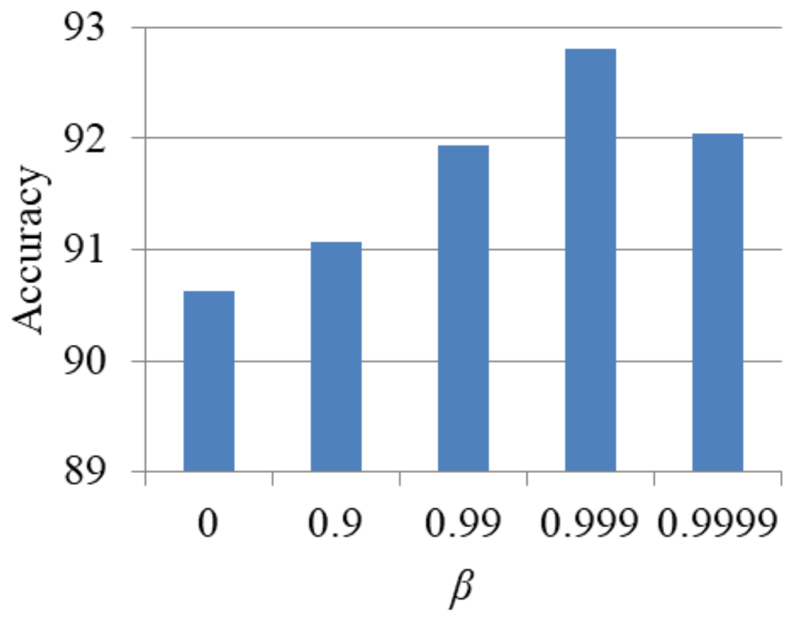
3.3. Class-Balanced Loss

Different categories of ships have different uses and demands. Thus, the number of ships in the real world varies greatly. As a result, the number of images of different ship categories in the optical remote sensing image dataset is also very unbalanced. The large sample data is dominant and affects the small sample when the loss function is not constrained. The training of large sample data will be greatly compressed when the function is constrained. Therefore, an appropriate constraint method should be found. In response to this problem, this paper uses the effective number of samples for each category to rebalance the loss, resulting in a CB loss.

The effective number of samples refers to the number of samples that do not overlap in features, which are in the feature space of one image category. There are two situations when adding a new sample to the dataset, as shown in Figure 8. They are overlapping with the original sample or non-overlapping with the original sample. The sum of all non-overlapping sample numbers is the effective number of samples $N$. The effective number of samples is more explanatory for the dataset than the total number of samples. CB loss solves the problem of unbalanced data training by introducing a weighting factor ${\alpha }_i\propto 1/E_{n_i}$, that is inversely proportional to the effective number of samples.

We normalize ${\alpha }_i$ as ${\displaystyle \sum _{i=1}^c}{\alpha }_i=C$ to make the total loss roughly in the same range when it works, and we use $1/E_{n_i}$ to denote the standardized weighting factor later.

Given a class $i$ sample with $n$ samples, we add a weighting factor $\left(1-\beta \right)/\left(1-{\beta }^{n_i}\right)$ to the loss function, of which hyper-parameter is $\beta =\left(N-1\right)/N$, and $\beta \in \left[0,1\right)$. The CB loss function is shown in Equation (12).

$$\mathrm{CB}\left(\mathrm{P},y\right)=\frac{1}{E_{n_y}}\mathcal{L}\left(\mathrm{P},y\right)=\frac{\left(1-\beta \right)}{\left(1-{\beta }^{{\mathrm{n}}_{\mathrm{y}}}\right)}\mathcal{L}\left(\mathrm{P},y\right)$$

(12)

where $n_y$ is the number of samples in the ground-truth class $y$. We make $\beta =0$ when there is no re-weighting. Conversely, $\beta \to 1$ is corresponding to re-weighing by inverse class frequency. $\mathcal{L}$ is the original loss function.

In this paper, the softmax cross-entropy loss is used as a benchmark. The softmax cross-entropy loss function is shown in Equation (13).

$${\mathrm{CE}}_{soft\max }\left(\mathrm{z},y\right)=-\log \left(\frac{\exp \left(z_y\right)}{{\displaystyle {\sum }_{j=1}^C\exp \left(z_j\right)}}\right)$$

(13)

where $z$ is the model prediction output and $C$ is the total number of classes. The probability distribution of all classes is calculated as $p_i=\exp \left(z_i\right)/{\displaystyle {\sum }_{j=1}^C\exp \left(z_j\right),\forall i\in \left\{1,2,\cdots ,C\right\}}$.

Suppose class $y$ has $n_y$ training samples, the class-balanced (CB) softmax cross-entropy loss is:

$${\mathrm{CB}}_{soft\max }\left(\mathrm{z},y\right)=-\frac{1-\beta }{1-{\beta }^{n_y}}\log \left(\frac{\exp \left(z_y\right)}{{\displaystyle {\sum }_{j=1}^C\exp \left(z_j\right)}}\right)$$

(14)

The influence of hyper-parameter $\beta$ on the accuracy will be discussed in the ablation experiment.

4. Experiments and Discussion

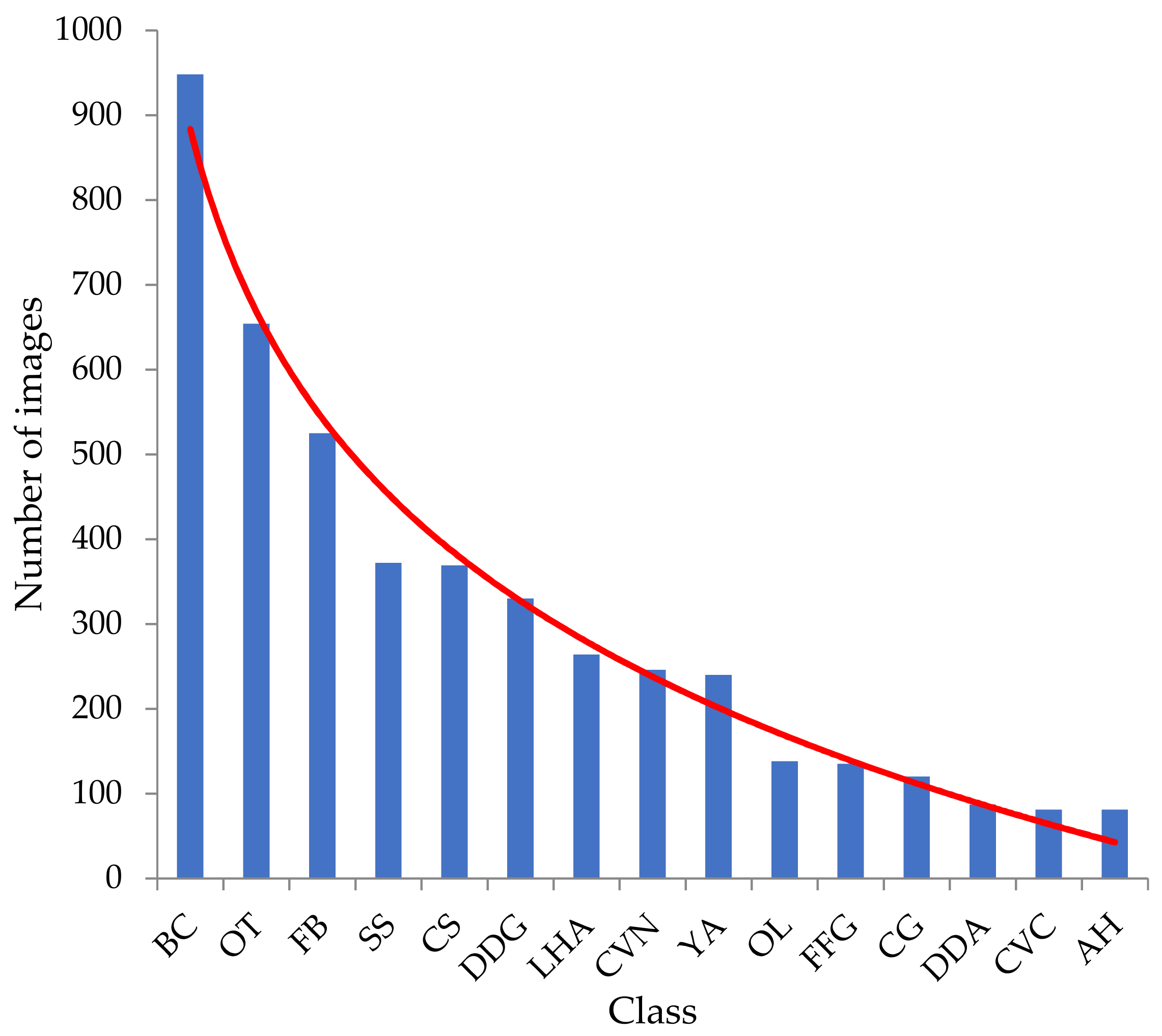
4.1. Dataset and Image Processing

4.1.1. Dataset

The existing optical remote sensing image datasets mainly focus on coarse-grained classification and target detection. Some of the publicly available fine-grained remote sensing ship datasets also have flaws. In order to get a more scientific result, we created a new dataset as the main experimental dataset. The other two available datasets are used to verify robustness in Section 4.7. The new fine-grained optical remote sensing ship classification dataset is called ORSC-15, which includes 15 types of ships. The optical remote sensing image format in the dataset is BMP. The image pixel size is 40–1200, and the resolution is sub-meter-3 m. The number of images in the training set is 3657, and the number of images in the test set is 933. Data sources include Google Earth (https://earth.google.com/web/ (accessed on 1 March 2021)), FGSC-23 dataset [1], HRSC2016 dataset [28], NWPU-RESISC45 dataset [29], and NWPU VHR-10 dataset [30]. We screen and crop images to ensure that all images meet fine-grained classification requirements. The categories of ships in the dataset are divided into bulk carrier (BC), container ship (CS), oil tanker (OT), ferry boat (FB), ocean liner (OL), yacht (YA), nuclear-powered aircraft carrier (CVN), conventionally-powered aircraft carrier (CVC), guided missile cruiser (CG), guided missile destroyer (DDG), anti-submarine destroyer (DDA), guided missile frigate (FFG), amphibious assault ship (LHA), submarine (SS) and hospital ship (AH), etc. Some of the warship category codes are from US Hull Classification Symbols. Various ship categories and sample images are shown in

Table 1. All ship categories and original images in the dataset. The backgrounds and resolutions of the images in the datasets vary.

Class	Example Image		Class	Example Image		Class	Example Image
BC			CS			FB
OL			OT			YA
AH			CVN			CVC
LHA			DDA			SS
FFG			DDG			CG

.

We comprehensively consider the two aspects in the process of establishing the dataset. (1) Our dataset includes the categories of ships with a large number and the categories of ships with a small number but have strategic significance. The former categories are represented by bulk carriers and container ships, while the latter include hospital ships and anti-submarine destroyers. (2) The background of remote sensing images is complex and diverse. It includes ocean background, sea land background and some other interfering objects. The dataset is randomly divided into the training set and test set according to the ratio of 8:2. Each class of images in the dataset is divided according to this scale. The images in the training and test sets do not overlap.

The dataset is divided into 15 categories of ships, as shown in

Table 2. Number of images in each category in the ORCS-15 dataset. The total number of ORSC-15 dataset is 4950.

Category	BC	CS	FB	OL	OT	YA	AH	CVN
Number	948	369	525	138	654	240	81	246
Category	CVC	LHA	DDA	SS	FFG	DDG	CG	Total
Number	81	264	87	372	135	330	120	4590

. 1530 images were collected in the dataset. On this basis, the same proportion of amplification was carried out. The final total number is 4590 and the format of images is JPG. Due to the large differences in the number of ships of each category in the real world, there is even an order of magnitude difference in the number of remote sensing images under different categories. Figure 9 is a histogram of the number of all ship categories in the dataset. This histogram can clearly show the long-tail distribution problem of the dataset caused by the imbalance of ship categories. The number of each category is detailed in Table 2.

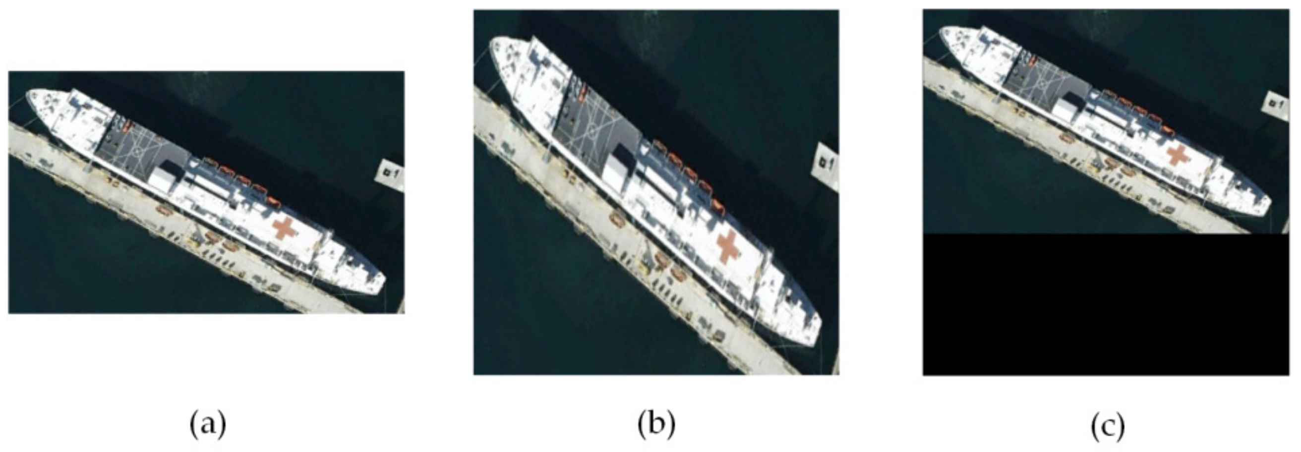
4.1.2. Image Processing

The image enhancement technology is used to expand the dataset in the control group. The image enhancement methods in this paper include image reversal, rotation, shear, displacement, and so on.

The original images have different sizes. Therefore, images of different shapes need resizing. Generally, the image is adjusted to a fixed size by interpolation or downsampling. However, this will destroy the original features of the image and lead to the imbalance of the ship captain aspect ratio. The image resizing operation of zero-padding is used in this paper. The longer edge of the image is first upsampled or downsampled to 224. Next, the shorter edges of the image are upsampled or subsampled at the same ratio. Finally, the rest of the image area is padded with zeros. The results of the two image size adjustment methods are shown in Figure 10. The adjustment method of zero-padding in Figure 10c retains more information than the subsampling in Figure 10b.

Zero-padding is also used to adjust the size consistently in the extraction process after ship positioning.

4.2. Implementation Details

The computer used in the experiment was configured with an Intel i7 processor and the graphics card is NVDIA RTX 3070s. The deep learning framework was Pytorch. ResNet50 [31] was used as the basic network to locate the target area of the ship. The size of the input images was unified to 256 × 256. The ResNet50 was pre-trained on the remote sensing ship dataset. The cropped ship positioning images were unified in size 224 × 224. Then the image of key parts was cropped and filled to the same size. Finally, feed them into the feature extraction network. We used backpropagation on the forward network. The proposed network is trained through stochastic gradient descent optimization when the momentum was 0.9, the learning rate was 0.01 and the batch size was 8. The training epoch was 100.

In the experiment, accuracy and recall are used as the evaluation indicators for fine-grained classification. Accuracy is the ratio of the correctly predicted images to all images in the test set. Equation (15) is the calculation method of the accuracy rate.

$$Accuracy=\frac{TP+TN}{TP+TN+FP+FN}$$

(15)

The confusion matrix (CM) [32] is the visualization of the classification matrix. The recall rate of each category can be seen from the CM. It is the ratio of the number of samples correctly identified as positive by the model to the total number of positive samples. In general, the higher the recall, the more positive samples are predicted correctly by the model. This means the model is more accurate. Equation (16) is the calculation method of the recall rate.

$$Recall=\frac{TP}{TP+FN}$$

(16)

where, true positive (TP) is a sample determined as positive and actually positive, and true negative (TN) is a sample determined as negative and actually negative. Correspondingly, false positive (FP) is a sample determined to be positive but actually negative, false negative (FN) is a sample determined to be negative but actually positive.

4.3. Visualization of Results

4.3.1. Feature Visualization

Figure 11 shows the Grad-CAM visualization of some images in the dataset. It can be seen that the model has a good effect on the positioning of the ship in the image, which is fine-tuned on the optical remote sensing ship dataset. Grad-CAM can help to eliminate interference from the irrelevant background.

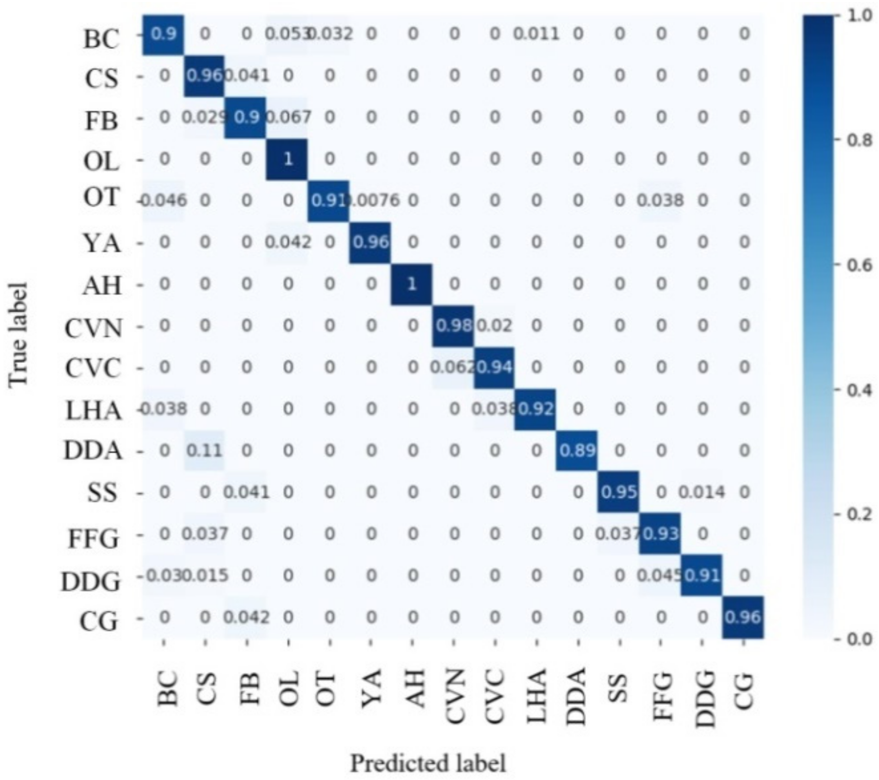
4.3.2. CM and Recall Rate

CM is the visualization of the classification matrix, which records the detailed classification results of each category. Each element in the CM represents the proportion predicted to be the n-th category but actually belongs to the m-th category. The recall rate of each category can be seen from the CM. The CM of the method which used in this paper is shown in Figure 12. The number on the diagonal is the recall rate. Among them, OL and AH have the highest recall rate. The recall rate of BC is low, and some samples are identified as OL, OT, and LHA. The single-type recall rate is not low overall. The rates indicate that this method can better classify the remote sensing ship dataset. The specific recall rate is shown in

Table 3. Recall rate of each category on ORSC-15 dataset. The recall rate of each category is relatively balanced, and the influence of the long-tailed distribution is reduced to a very low level.

Category	BC	CS	FB	OL	OT	YA	AH	CVN
Recall/%	0.9	0.96	0.9	1	0.91	0.96	1	0.98
Category	CVC	LHA	DDA	SS	FFG	DDG	CG
Recall/%	0.94	0.92	0.89	0.95	0.93	0.91	0.96

.

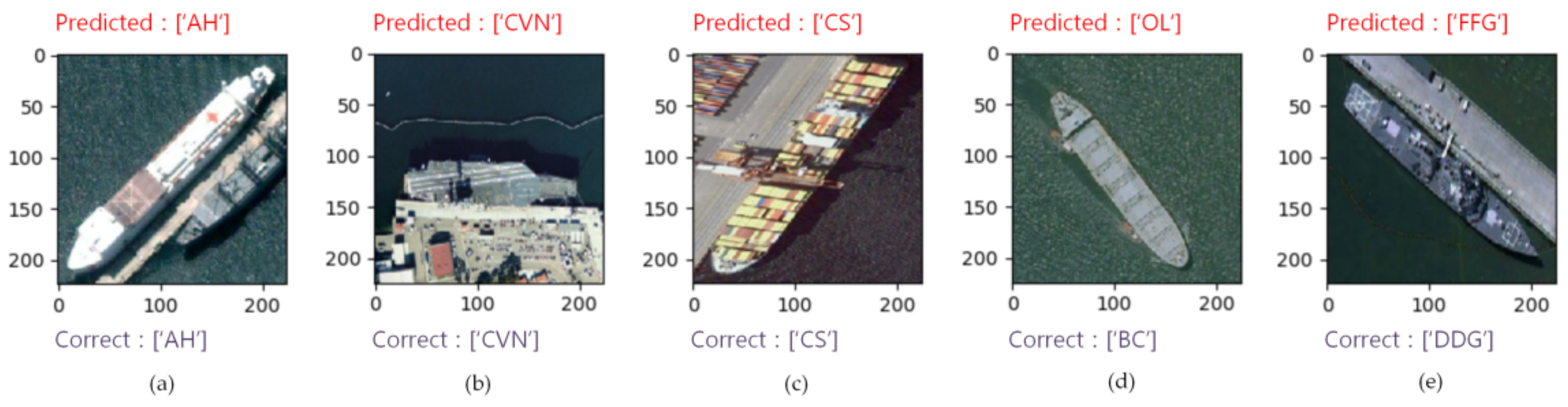
4.3.3. Display of Classification Results

The classification results of ships are shown in Figure 13. Figure 13a–c is the result of correct classification. Figure 13a is AH, Figure 13b is CVN, and Figure 13c is CS. Figure 13d,e are the results of misclassification. Figure 13d shows the misclassification of BC as OL. The reason is the inter-class similarity of these two types of ships. They all belong to large transport ships with similar aspect ratio. Specific to the BC in this image, its cargo hold of midship is more similar to an oil pipeline of the OL. Therefore, it is not correctly classified in our algorithm. In Figure 13e, the algorithm classifies the image as FFG. However, the correct class of the image is DDG. Including slender hulls, similar livery and poorly differentiated combat units can lead to misclassification. Moreover, some DDG and FFG remote sensing images are difficult to distinguish even by human eyes.

4.4. Ablation Experiment

In this subsection, we first investigate the effect of different downsampling rates on the accuracy in SC-conv. It can be seen that the performance is the best when DS Rate (r) is 4. We set r to be 4 in subsequent experiments. The experimental comparison results are shown in

Table 4. The effect of different sampling rates on the classification results. Bold values indicate best performance.

DS Rate (r)	1	2	3	4
Accuracy	92.48	92.70	92.70	92.81

.

We use Grad-CAM to locate the ship in the image to eliminate irrelevant background interference. We designed an ablation experiment to verify the role of image localization and self-calibrating convolution in the algorithm. As shown in

Table 5. Comparison of classification performance of different modules. Bold values indicate best performance.

SC-conv		√	√	√	√	√
Target area positioning	√		√	√	√	√
Global features	√			√	√	√
Target-level features	√		√		√	√
Key part features	√		√	√		√
Accuracy/%	90.74	86.93	91.83	91.72	90.08	92.81

, the accuracy of the algorithm drops significantly when the image positioning part is not added. The reason is that it cannot extract more detailed features for classification. After excluding SC-conv, the accuracy of the algorithm also decreased because more abundant output features could not be obtained.

We also verified the influence of input features at all levels on classification accuracy in the ablation experiment. First, we remove the input CNN part of the original image to verify the influence of the unchanged global features on the algorithm. The object-level features are the features of the image after the ship is localized. The key part features are the features of the midship part. Next, we verified the influence of these two features on the results. The experimental results are shown in Table 5. It shows the accuracy was improved by 2.73% after adding the key part features extraction module. The global features and target-level features bring 0.98% and 1.09% improvements to the experimental results. The experimental results show that each branch of the network has an impact on the classification results. Especially, the extraction of key part features has the highest improvement of accuracy.

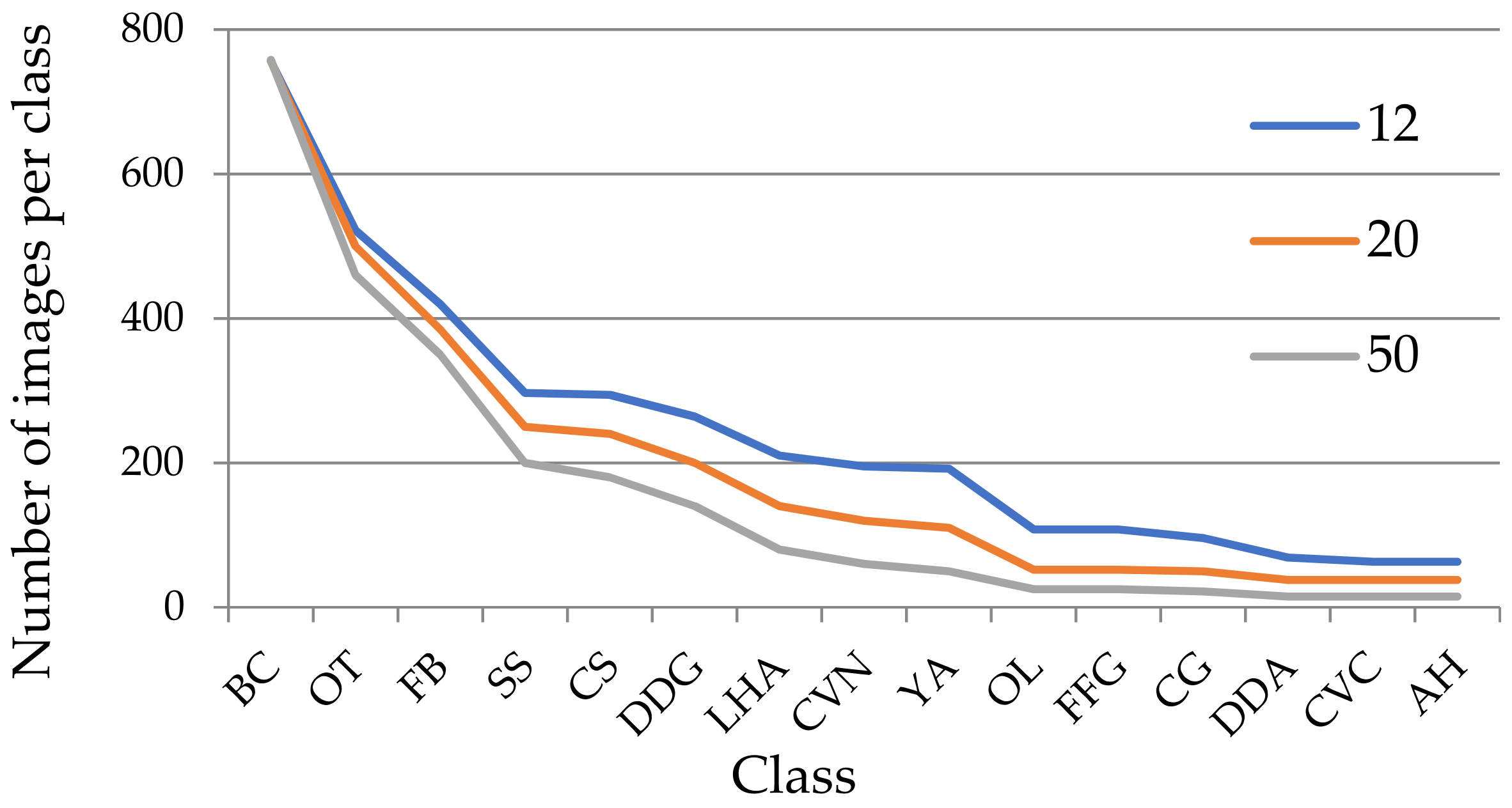
4.5. Long-Tailed Distribution Experiment

We set up another ablation experiment to analyze the impact of CB loss on the accuracy of ship classification. By adjusting the value of $\beta$, a higher classification accuracy of long tail data sets can be achieved. The value of $\beta$ generally takes [0.9–1). We pre-set the hyperparameter $\beta$ to 0, 0.9, 0.99, 0.999 and 0.9999. It is equivalent to no reweighting when $\beta =0$. $\beta \to 1$ corresponds to reweighting by inverse class frequency and is not discussed. The other parts of the network remain unchanged. The experimental results are shown in Figure 14. When the hyper-parameter $\beta$ is 0.999, the accuracy is the highest and 2.18% higher than that of no reweighting. Therefore, the experimental results show that the re-weighting method of CB loss in the process of image classification can effectively improve the accuracy of ship classification. The appropriate hyperparameters can not only improve accuracy, but also improve the adverse effects of long-tailed distributions. As shown in Table 3, our method also has a good learning effect on tail categories.

We also conducted related experiments on different imbalance factors. We take the ratio of the number of images of the largest class to the smallest class in the training set as the imbalance factor. We manually unbalance the training set of the ORSC-15 dataset, leaving the test set unchanged. Figure 15 shows the number of samples in each category of the training set with different imbalance factors. The accuracy drops somewhat when the classes are more imbalanced. As shown in

Table 6. Comparative experiments under different imbalance factors. The value of $\beta$ in the second column is the best value after comparison.

Imbalance Factor	β	Accuracy
12	0.999	92.81
20	0.999	89.40
50	0.99	83.92

, when the imbalance factor is expanded to 50, the hyperparameter $\beta$ = 0.99 works best.

4.6. Compared with Other State-of-the-Art Methods

We compared the proposed network with other state-of-the-art classification methods to analyze the classification performance of the network. The method in this paper has the highest accuracy rate of 92.81%. As shown in

Table 7. Compare with other state-of-the-art methods on ORSC-15 dataset. A check mark in the second column indicates that the method is a fine-grained method. Bold values indicate best performance.

Method	Fine Grained Network	Accuracy/%
VGG16		79.96
Inception V3		80.61
ResNet50		84.42
Bilinear CNN	√	88.76
RA-CNN	√	88.01
MA-CNN	√	89.22
WS-DAN	√	90.30
Ours (without Reweighting)	√	90.63
IICL-CNN		85.07
AMEFRN	√	91.07
Ours	√	92.81

, compared with classic network models such as VGG 16 [33], Inception V3 [34], and ResNet50 [31]; the accuracy rates are improved by 12.85%, 12.20%, and 8.39%, respectively. Compared with other fine-grained methods, it is 4.05% higher than Bilinear CNN. The reason is that Bilinear CNN does not capture key parts and has low accuracy. Compared with RACNN and MACNN, it is increased by 4.80% and 3.59%, respectively. WS-DAN combines weakly supervised learning and data expansion to achieve high accuracy. Compared with WS-DAN, the accuracy rate is increased by 2.51%. Compared with the two remote sensing ship classification methods IICL-CNN and AMEFRN, the accuracy is improved by 7.74% and 1.74%, respectively. The experimental results show this method has higher recognition accuracy on the remote sensing ship dataset when compared with other methods.

4.7. Robustness Test

In order to analyze the performance of the algorithm in more detail, we conducted experiments on the FGSC-23 dataset and the FGSCR-42 dataset [35]. The FGSC-23 dataset includes 22 categories of ships with a total of 3596 optical remote sensing images. The image format of the FGSC-23 dataset is JPG, the resolution is 0.4 m–2 m, and the pixel size is 40–800. In order to maintain the long tail feature and expand the validation data, we double this dataset with data augmentation. The training set has 5738 images, and the test set has 1454 images. The FGSCR-42 dataset includes a total of 7789 optical remote sensing images of different resolutions in 42 categories. The FGSCR-42 dataset has an image format of BMP and a pixel size of 40–800. There are deficiencies in the classification of samples in this dataset. Some categories have only two images. In order to unify the standards, we reclassify the dataset into 17 categories. The number of images per category varies from 226 to 1007. Among them, 80% of the images in the dataset are divided into the training set and 20% of the images are divided into the test set. To ensure fairness, various methods use the same scheme in related experiments.

The experimental results are shown in

Table 8. Compared with other state-of-the-art methods on FGSC-23 dataset. A check mark in the second column indicates that the method is a fine-grained method. Bold values indicate best performance.

Method	Fine Grained Network	Accuracy/%
VGG16		80.15
Inception V3		82.97
ResNet50		83.65
Bilinear CNN	√	84.48
RA-CNN	√	86.47
MA-CNN	√	88.60
WS-DAN	√	86.06
Ours (without Reweighting)	√	90.52
IICL-CNN		88.87
AMEFRN	√	92.10
Ours	√	93.54

and

Table 9. Compared with other state-of-the-art methods on FGSCR-42 dataset. A check mark in the second column indicates that the method is a fine-grained method. Bold values indicate best performance.

Method	Fine Grained Network	Accuracy/%
VGG16		84.21
Inception V3		86.20
ResNet50		84.66
Bilinear CNN	√	90.50
RA-CNN	√	90.95
MA-CNN	√	91.07
WS-DAN	√	90.56
Ours (without Reweighting)	√	92.17
IICL-CNN		89.99
AMEFRN	√	93.32
Ours	√	93.97

. This method has a good classification effect on different remote sensing ship datasets by comparing with other classification methods. Similarly, it has strong robustness in remote sensing ship image classification.

5. Conclusions

This paper discusses the task of fine-grained ship image classification in optical remote sensing datasets. A set of schemes is proposed to solve the problems of inter-class similarity between ships and long-tail distribution. We constructed a 15-category fine-grained remote sensing ship classification dataset to complete the verification of the task in this paper. We solve the problems of fine-grained remote sensing ship classification tasks in three aspects. They are the selection of specific distinctive parts, self-calibrating convolution and the re-weighting of samples. Specifically, we rely on Grad-CAM to locate the ship’s position to remove unnecessary interference. Then we chose the discriminative midship image to solve the problems of inter-class similarity and intra-class differences. Next, we use the self-calibrated convolutional network to expand the field of view of each convolutional layer and enrich the output features. We use the CB loss to deal with the long-tail problem of the remote sensing ship dataset to improve the classification accuracy. Experiments on different remote sensing ship datasets show that the accuracy of the model has reached 92.81%, 93.54% and 93.97%, respectively. Compared with other advanced methods, the experimental results show that this method has better classification performance and robustness. We plan to further study the issue of feature fusion in future work to improve accuracy. Finally, it is hoped that the fine-grained remote sensing ship classification method can make greater progress in weakly supervised learning and play an important role in the marine field. Our code will be published at https://github.com/SPQCN/REMOTE-SENSING (accessed on 31 July 2022) after the related work is completed.

References

1. Zhang, X.; Lv, Y.; Yao, L.; Xiong, W.; Fu, C. A New Benchmark and an Attribute-Guided Multilevel Feature Representation Network for Fine-Grained Ship Classification in Optical Remote Sensing Images. IEEE J. Sel. Top. Appl. Earth Obs. Remote Sens. 2020, 13, 1271–1285. [Google Scholar] [CrossRef]
2. Antelo, J.; Ambrosio, G.; Gonzalez, J.; Galindo, C. Ship detection and recognitionin high-resolution satellite images. In Proceedings of the 2009 IEEE International Geoscience and Remote Sensing Symposium (IGARSS), Cape Town, South Africa, 12–17 July 2009; pp. IV-514–IV-517. [Google Scholar]
3. Selvi, M.U.; Kumar, S.S. A Novel Approach for Ship Recognition Using Shape and Texture. Int. J. Adv. Inf. Technol. (IJAIT) 2011, 1. [Google Scholar] [CrossRef]
4. Leng, X.; Ji, K.; Zhou, S.; Xing, X.; Zou, H. A comb feature for the analysis of ship classification in high resolution SAR imagery. In Proceedings of the 2016 CIE International Conference on Radar (RADAR), Guangzhou, China, 10–13 October 2016; pp. 1–4. [Google Scholar]
5. Wang, Q.; Gao, X.; Chen, D. Pattern Recognition for Ship Based on Bayesian Networks. In Proceedings of the Fourth International Conference on Fuzzy Systems and Knowledge Discovery (FSKD 2007), Haikou, China, 24–27 August 2007; pp. 684–688. [Google Scholar]
6. Lang, H.; Wu, S.; Xu, Y. Ship Classification in SAR Images Improved by AIS Knowledge Transfer. IEEE Geosci. Remote Sens. Lett. 2018, 15, 439–443. [Google Scholar] [CrossRef]
7. Chen, J.; Qian, Y. Hierarchical Multilabel Ship Classification in Remote Sensing Images Using Label Relation Graphs. IEEE Trans. Geosci. Remote Sens. 2022, 60, 5611513. [Google Scholar] [CrossRef]
8. Shi, Q.; Li, W.; Tao, R. 2D-DFrFT Based Deep Network for Ship Classification in Remote Sensing Imagery. In Proceedings of the 2018 10th IAPR Workshop on Pattern Recognition in Remote Sensing (PRRS), Beijing, China, 19–20 August 2018; pp. 1–5. [Google Scholar]
9. Liu, K.; Yu, S.; Liu, S. An Improved InceptionV3 Network for Obscured Ship Classification in Remote Sensing Images. IEEE J. Sel. Top. Appl. Earth Observ. Remote Sens 2020, 13, 4738–4747. [Google Scholar] [CrossRef]
10. Chen, J.; Chen, K.; Chen, H.; Li, W.; Zou, Z.; Shi, Z. Contrastive Learning for Fine-Grained Ship Classification in Remote Sensing Images. IEEE Trans. Geosci. Remote Sens. 2022, 60, 4707916. [Google Scholar] [CrossRef]
11. Xiong, W.; Xiong, Z.; Cui, Y. An Explainable Attention Network for Fine-Grained Ship Classification Using Remote-Sensing Images. IEEE Trans. Geosci. Remote Sens. 2022, 60, 5620314. [Google Scholar] [CrossRef]
12. Hu, T.; Qi, H. See Better Before Looking Closer: Weakly Supervised Data Augmentation Network for Fine-Grained Visual Classification. arXiv 2019, arXiv:1901.09891. [Google Scholar]
13. Liu, J.J.; Hou, Q.; Cheng, M.M.; Wang, C.; Feng, J. Improving Convolutional Networks with Self-Calibrated Convolutions. In Proceedings of the 2020 IEEE/CVF Conference on Computer Vision and Pattern Recognition (CVPR), Seattle, WA, USA, 13–19 June 2020; pp. 10093–10102. [Google Scholar]
14. Zhang, N.; Donahu, J.; Girshick, R.; Darrell, T. Part-based R-CNNs for fine-grained category detection. In Proceedings of the Computer Vision—ECCV 2014, Zurich, Switzerland, 6–12 September 2014; Volume 8689, pp. 834–849. [Google Scholar]
15. Branson, S.; Horn, G.V.; Belongie, S.; Perona, P. Bird species categorization using pose normalized deep convolutional nets. arXiv 2014, arXiv:1406.2952. [Google Scholar]
16. Xiao, T.; Xu, Y.; Yang, K.; Zhang, J.; Peng, Y.; Zhang, Z. The application of two-level attention models in deep convolutional neural network for fine-grained image classification. In Proceedings of the 2015 IEEE Conference on Computer Vision and Pattern Recognition (CVPR), Boston, MA, USA, 7–12 June 2015; pp. 842–850. [Google Scholar]
17. Zheng, H.; Fu, J.; Mei, T.; Luo, J. Learning Multi-attention Convolutional Neural Network for Fine-Grained Image Recognition. In Proceedings of the 2017 IEEE International Conference on Computer Vision (ICCV), Venice, Italy, 22–29 October 2017; pp. 5219–5227. [Google Scholar]
18. Wang, Y.; Morariu, V.I.; Davis, L.S. Learning a Discriminative Filter Bank Within a CNN for Fine-Grained Recognition. In Proceedings of the 2018 IEEE/CVF Conference on Computer Vision and Pattern Recognition (CVPR), Salt Lake City, UT, USA, 18–23 June 2018; pp. 4148–4157. [Google Scholar]
19. Chen, Y.; Bai, Y.; Zhang, W.; Mei, T. Destruction and Construction Learning for Fine-Grained Image Recognition. In Proceedings of the 2019 IEEE/CVF Conference on Computer Vision and Pattern Recognition (CVPR), Long Beach, CA, USA, 15–20 June 2019; pp. 5152–5161. [Google Scholar]
20. Yu, C.; Zha, X.; Zheng, Q.; Zhang, P.; You, X. Hierarchical Bilinear Pooling for Fine-Grained Visual Recognition. In Proceedings of the Computer Vision—ECCV 2018, Munich, Germany, 8–14 September 2018; Volume 11220, pp. 595–610. [Google Scholar]
21. Kong, S.; Fowlkes, C. Low-Rank Bilinear Pooling for Fine-Grained Classification. In Proceedings of the 2017 IEEE Conference on Computer Vision and Pattern Recognition (CVPR), Honolulu, HI, USA, 21–26 July 2017; pp. 7025–7034. [Google Scholar]
22. Fu, J.; Zheng, H.; Mei, T. Look Closer to See Better: Recurrent Attention Convolutional Neural Network for Fine-Grained Image Recognition. In Proceedings of the 2017 IEEE Conference on Computer Vision and Pattern Recognition (CVPR), Honolulu, HI, USA, 21–26 July 2017; pp. 4476–4484. [Google Scholar]
23. Zhou, B.; Khosla, A.; Lapedriza, A.; Oliva, A.; Torralba, A. Learning Deep Features for Discriminative Localization. In Proceedings of the 2016 IEEE Conference on Computer Vision and Pattern Recognition (CVPR), Las Vegas, NV, USA, 27–30 June 2016; pp. 2921–2929. [Google Scholar]
24. Selvaraju, R.R.; Cogswell, M.; Das, A.; Vedantam, R.; Parikh, D.; Batra, D. Grad-CAM: Visual Explanations from Deep Networks via Gradient-Based Localization. In Proceedings of the 2017 IEEE International Conference on Computer Vision (ICCV), Venice, Italy, 22–29 October 2017; pp. 618–626. [Google Scholar]
25. Wang, Y.; Gan, W.; Yang, J.; Wu, W.; Yan, J. Dynamic Curriculum Learning for Imbalanced Data Classification. In Proceedings of the 2019 IEEE/CVF International Conference on Computer Vision (ICCV), Seoul, Korea, 27 October–2 November 2019; pp. 5016–5025. [Google Scholar]
26. Cui, Y.; Jia, M.; Lin, T.; Song, Y.; Belongie, S. Class-Balanced Loss Based on Effective Number of Samples. In Proceedings of the 2019 IEEE/CVF Conference on Computer Vision and Pattern Recognition (CVPR), Long Beach, CA, USA, 15–20 June 2019; pp. 9260–9269. [Google Scholar]
27. Liu, J.; Sun, Y.; Han, C.; Dou, Z.; Li, W. Deep Representation Learning on Long-Tailed Data: A Learnable Embedding Augmentation Perspective. In Proceedings of the 2020 IEEE/CVF Conference on Computer Vision and Pattern Recognition (CVPR), Seattle, WA, USA, 13–19 June 2020; pp. 2967–2976. [Google Scholar]
28. Liu, Z.; Yuan, L.; Weng, L.; Yang, Y. A High Resolution Optical Satellite Image Dataset for Ship Recognition and Some New Baselines. In Proceedings of the 6th International Conference on Pattern Recognition Applications and Methods (ICPRAM), Porto, Portugal, 24–26 February 2017; Volume 1, pp. 324–331. [Google Scholar]
29. Cheng, G.; Han, J.; Lu, X. Remote Sensing Image Scene Classification: Benchmark and State of the Art. Proc. IEEE 2017, 105, 1865–1883. [Google Scholar] [CrossRef]
30. Cheng, G.; Han, J.; Zhou, P.; Guo, L. Multi-class geospatial object detection and geographic image classification based on collection of part detectors. ISPRS-J. Photogramm. Remote Sens. 2014, 98, 119–132. [Google Scholar] [CrossRef]
31. He, K.; Zhang, X.; Ren, S.; Sun, J. Deep Residual Learning for Image Recognition. In Proceedings of the 2016 IEEE Conference on Computer Vision and Pattern Recognition (CVPR), Las Vegas, NV, USA, 27–30 June 2016; pp. 770–778. [Google Scholar]
32. Ohsaki, M.; Wang, P.; Matsuda, K.; Katagiri, S.; Watanabe, H.; Ralescu, A. Confusion-Matrix-Based Kernel Logistic Regression for Imbalanced Data Classification. IEEE Trans. Knowl. Data Eng. 2017, 29, 1806–1819. [Google Scholar] [CrossRef]
33. Simonyan, K.; Zisserman, A. Very deep convolutional networks for large-scale image recognition. In Proceedings of the 2015 International Conference on Learning Representations (ICLR), San Diego, CA, USA, 7–9 May 2015; pp. 1–14. [Google Scholar]
34. Szegedy, C.; Vanhoucke, V.; Ioffe, S.; Shlens, J.; Wojna, Z. Rethinking the Inception Architecture for Computer Vision. In Proceedings of the 2016 IEEE Conference on Computer Vision and Pattern Recognition (CVPR), Las Vegas, NV, USA, 27–30 June 2016; pp. 2818–2826. [Google Scholar]
35. Di, Y.; Jiang, Z.; Zhang, H. A Public Dataset for Fine-Grained Ship Classification in Optical Remote Sensing Images. Remote Sens. 2021, 13, 747. [Google Scholar] [CrossRef]
Figure 1. (a) Inter-class similarity, take ocean liner and ferry boat for example. (b) Intra-class differences, taking different container ships as an example, the position of the bridge is marked with red circles.
Remotesensing 14 04566 g001
Figure 2. Comparison of midship images in different ships. (a,b) are container ships; (c) is a nuclear-powered aircraft carrier; (df) are guided missile frigates, guided missile destroyers and guided missile cruisers, respectively; (a,b) show that the midships of ships of the same type are highly similar; (cf) show that the midship parts of different types of ships are quite different.
Remotesensing 14 04566 g002
Figure 3. The framework of the proposed network. (a) Ship positioning network based on Grad-CAM; (b) two-stage image extraction network; (c) self-calibrated convolutions network; (d) feature fusion. First, we locate the ship image. The positioning image is then masked. The resulting different images are fed into a feature extraction network and classified.
Remotesensing 14 04566 g003
Figure 4. Visualization of Grad-CAM results. (a) Original remote sensing ship image. (b) Grad-CAM visualization image. The red part is the focus area. (c) Overlay of the visualized image with the original image. The area of focus is the ship location.
Remotesensing 14 04566 g004
Figure 5. The class activation map of ship is obtained through Grad-CAM. Grad-CAM finds the gradient of the last layer of the convolutional layer, and the average value of the gradient is the weight of the feature map. Then, calculate the weighted sum to get the class activation map.
Remotesensing 14 04566 g005
Figure 6. Using affine transformation to extract ship target-level image. (a) is the object positioning image p x , y ; (b) is the target image. Affine transformation can reduce the background information interference in the target image.
Remotesensing 14 04566 g006
Figure 7. Schematic illustration of the self-calibrated convolutions. The original filter is separated into four parts, each responsible for different functions. The plus sign in the figure is element-wise summation. The dots in the figure are element-wise multiplication.
Remotesensing 14 04566 g007
Figure 8. Two cases of adding new samples to dataset. In the first case, the new sample does not overlap with the previously sampled data. In the second case, the new sample overlaps with the previously sampled data.
Remotesensing 14 04566 g008
Figure 9. Long tail distribution of remote sensing ship dataset. The abscissa is the ship class, and the ordinate is the number of images. The red line represents the long-tailed distribution trend.
Remotesensing 14 04566 g009
Figure 10. Different size adjustment methods. (a) is the original image; (b,c) are downsampling and zero-padding methods, respectively. The zero-padding method in (c) preserves more ship shape information than the method in (b).
Remotesensing 14 04566 g010
Figure 11. Grad-CAM visualization of remote sensing ship images. (ac) are the visualization results of YA, AH and LHA, respectively. It can be seen that Grad-CAM can locate the ship in the image very well.
Remotesensing 14 04566 g011
Figure 12. Confusion matrix of classification results of each category. The horizontal axis is the predicted label, and the vertical axis is the true label. Darker colors correspond to larger values.
Remotesensing 14 04566 g012
Figure 13. Classification results for AH, CVN, CS, BC and DDG. (ac) are visualizations of the correct classification results; (d,e) are visualizations of misclassification results.
Remotesensing 14 04566 g013
Figure 14. Hyper-parameter β impact on classification accuracy.
Remotesensing 14 04566 g014
Figure 15. The number of samples in each category of the training set with imbalance factors of 12, 20 and 50. The blue line represents a factor of 12, the orange line represents a factor of 20, and the gray line represents a factor of 50.
Remotesensing 14 04566 g015