
On-Orbit Autonomous Geometric Calibration of Directional Polarimetric Camera
by
 ,
,
Guangfeng Xiang
1,2,3,
Binghuan Meng
1,3,*,
Bihai Tu
1,3,
Xuefeng Lei
1,2,3,
Tingrui Sheng
1,2,3,
Lin Han
1,3,
Donggen Luo
1,3 and
Jin Hong
1,3 1
Anhui Institute of Optics and Fine Mechanics, Hefei Institutes of Physical Science, Chinese Academy of Sciences, Hefei 230031, China
2
University of Science and Technology of China, Hefei 230026, China
3
Key Laboratory of Optical Calibration and Characterization, Chinese Academy of Sciences, Hefei 230031, China
*
Author to whom correspondence should be addressed.
Remote Sens. 2022, 14(18), 4548; https://doi.org/10.3390/rs14184548
Submission received: 28 July 2022
/
Revised: 5 September 2022
/
Accepted: 8 September 2022
/
Published: 12 September 2022
(This article belongs to the Topic Advances in Environmental Remote Sensing)
Abstract
:The Directional Polarimetric Camera (DPC) carried by the Chinese GaoFen-5-02 (GF-5-02) satellite has the ability for multiangle, multispectral, and polarization detection and will play an important role in the inversion of atmospheric aerosol and cloud characteristics. To ensure the validity of the DPC on-orbit multiangle and multispectral polarization data, high-precision image registration and geolocation are vital. High-precision geometric model parameters are a prerequisite for on-orbit image registration and geolocation. Therefore, on the basis of the multiangle imaging characteristics of DPC, an on-orbit autonomous geometric calibration method without ground reference data is proposed. The method includes three steps: (1) preprocessing the original image of the DPC and the satellite attitude and orbit parameters; (2) scale-invariant feature transform (SIFT) algorithm to match homologous points between multiangle images; (3) optimization of geometric model parameters on-orbit using least square theory. To verify the effectiveness of the on-orbit autonomous geometric calibration method, the image registration performance and relative geolocation accuracy before and after DPC on-orbit geometric calibration were evaluated and analyzed using the SIFT algorithm and the coastline crossing method (CCM). The results show that the on-orbit autonomous geometric calibration effectively improves the DPC image registration and relative geolocation accuracy. After on-orbit calibration, the multiangle image registration accuracy is better than 1.530 km, the multispectral image registration accuracy is better than 0.650 km, and the relative geolocation accuracy is better than 1.275 km, all reaching the subpixel level (<1.7 km).
1. Introduction
On 7 September 2021, China successfully launched the GaoFen-5-02 (GF-5-02) satellite into a predetermined sun-synchronous orbit with a CZ-4C-Y40 carrier rocket at the Taiyuan Satellite Launch Center, with a nominal orbit altitude of 705 km. The satellite carries two Earth observation payloads and five atmospheric sounding payloads: Advanced Hyperspectral Imager (AHSI) [1], Visual and Infrared Multispectral Imager (VIMI) [2], Greenhouse Gas Monitoring Instrument (GMI) [3], Environment Monitoring Instrument (EMI) [4], Directional Polarization Camera (DPC) [5,6,7,8,9], Particulate Observing Scanning Polarimeter (POSP) [5], and Absorptive Aerosol Sensor (AAS) [10]. Through the cooperation of various payloads, China’s hyperspectral observation capacity in the atmosphere, water, and land will be comprehensively improved, meeting the urgent needs of China’s comprehensive environmental monitoring and providing effective data guarantee for environmental protection operations such as atmospheric environment monitoring, water environment monitoring, and ecological environment monitoring.
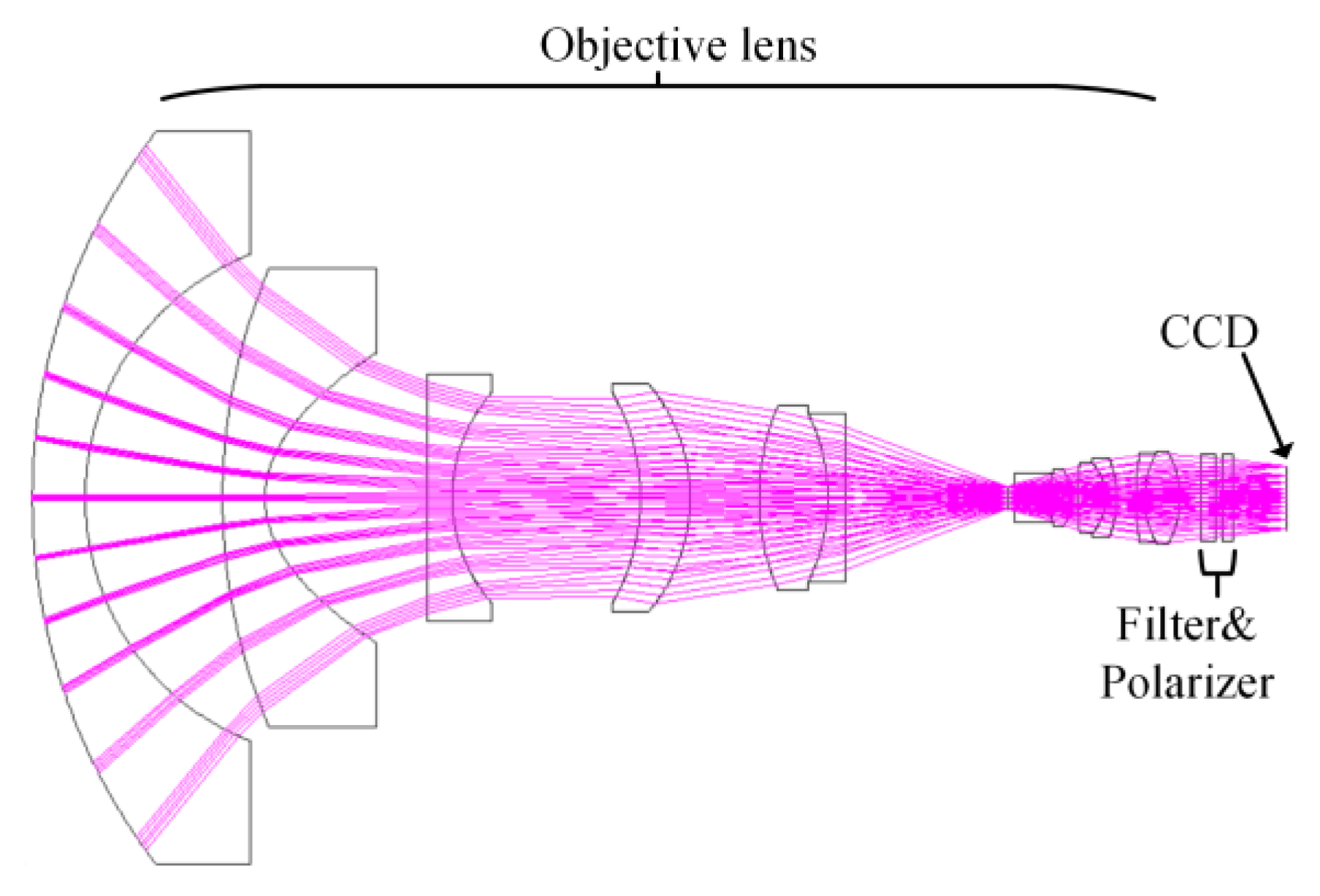
Among them, the DPC developed by the Anhui Institute of Optics and Fine Mechanics (AIOFM) of the Chinese Academy of Sciences (CAS) has multiangle, multispectral, and polarization detection capabilities. Combined with the inversion model of atmospheric properties based on polarization information, the DPC will play an important role in the inversion of atmospheric aerosol and cloud parameters [11,12,13]. In addition to the already launched GF-5-01, GF-5-02, and DQ-1 satellites, subsequent CM satellites are also planned to carry DPC. As shown in Figure 1, the DPC optical system consists of an objective lens, a filter and polarizer wheel, and an area array charge-coupled device (CCD). The design concept is similar to the French Polarization and Directionality of the Earth Reflectances (POLDER) [14,15,16,17,18] series of instruments. The objective lens has a wide field of view (FOV) and image space telecentric characteristics. The wide FOV imaging capability based on DPC can observe the target from multiple angles along the track. The design of the image space telecentric ensures that there is enough space to install the filter and polarizer wheel. The filter and polarizer wheel adopt the time-sharing detection mode, which can analyze the multispectral and polarized radiation information of the target. The area array CCD is used to complete the photoelectric conversion of remote sensing images, and it should meet the design requirements of the instrument’s working band, dynamic range, and spatial resolution. Table 1 shows the DPC parameters to be configured for each satellite. The GF-5-02 and DQ-1 satellites use a 2 × 2 pixel combination to ensure the same nadir resolution as the GF-5-01 satellite. The follow-up research object of this paper is the DPC carried by the GF-5-02 satellite.
To take full advantage of the multiangle and multispectral polarization detection advantages of DPC, not only are radiation and polarization detection accuracy required, but high-precision image registration and geolocation are also extremely important. Therefore, it is necessary to establish the mapping relationship between object points in 3D space and image points on the instrument’s 2D image plane with high-precision geometric calibration. The geometric calibration of spaceborne optical instruments is generally divided into two stages: pre-launch laboratory geometric calibration and on-orbit geometric calibration. The geometric model parameters calibrated by the laboratory cannot effectively represent the geometric performance of the instrument on-orbit because of the violent vibration during launch and the difference between the on-orbit environment and the laboratory environment. Therefore, the validity of on-orbit observation data of spaceborne optical instruments depends largely on high-precision on-orbit geometric calibration. Traditional on-orbit geometric calibration methods are usually based on the reference data of high-precision ground calibration fields [19,20]. The ground calibration field can provide satellites with ground control points with high-precision geographic coordinate information as an absolute reference for on-orbit geometric calibration. This method matches the calibration field image acquired by the on-orbit instrument with the reference image and then realizes the on-orbit geometric calibration using dense control point constraint. However, due to the dependence on calibration field reference data, this method has the opportunity to calibrate only when the satellite passes through the calibration field, and its timeliness is greatly limited. The calibration field size is usually only tens to hundreds of kilometers, for DPC, which is a spaceborne optical instrument with a swath width of thousands of kilometers, the ground calibration field cannot be used for all-around on-orbit geometric calibration. To solve the limitations of the traditional on-orbit geometric calibration method based on a ground calibration field, it is urgent to explore an on-orbit autonomous geometric calibration method without reference data from the ground calibration field. In the field of computer vision, camera autonomous calibration methods have always been a hot research topic [21,22,23,24]. In the field of satellite remote sensing, on-orbit autonomous geometric calibration methods have also attracted more and more attention from researchers in recent years [17,25,26,27,28]. Gresloud et al. [25], on the basis of the agile imaging capabilities of the Pleiades [29], used two imaging methods of along-track push-broom and cross-track swing-scanning to obtain cross images with a yaw angle difference of nearly 90° during a satellite transit. Then, the on-orbit autonomous geometric calibration was carried out according to the geometric constraint relationship of the homologous points between the cross images. However, the corresponding calibration model and solution method were not described in detail in [25]. Moreover, the calibration method requires the satellite to have agile imaging ability, which is not suitable for satellites without agile imaging ability (such as GF-5-01 satellite, GF-5-02 satellite, DQ-1 satellite, and CM satellite). Wang et al. [26] proposed an on-orbit geometric calibration method based on two ground control points and homologous points evenly distributed between the two images in their research on the on-orbit geometric calibration of the GaoFen-4 satellite. Although this method greatly reduces the need for ground control points compared with the traditional on-orbit geometric calibration method based on the ground calibration field, there is still a gap with the on-orbit autonomous geometric calibration method (no ground control points at all) we pursue. Zhang et al. [27] proposed using at least three images with overlapping regions to match homologous points and calculate the internal distortion of the instrument according to the forward intersection residual between the homologous points. However, this method only considers the calibration of the internal distortion of the spaceborne push-broom instrument. Fougnie et al. [17] proposed that the multiangle detection capability based on Polarization and Anisotropy of Reflectance for Atmospheric Sciences coupled with Observations from a Lidar (PARASOL) can perform on-orbit autonomous geometric calibration of the instrument installation angle error, but there is no public calibration model and specific implementation method. In a word, there are relatively few studies on the on-orbit autonomous geometric calibration methods in the field of satellite remote sensing, especially for instruments similar to DPC with a wide FOV, low resolution, and area array imaging. However, the DPC’s multiangle imaging capability along the track makes it possible for its on-orbit autonomous geometric calibration.
In this paper, a geometric model of on-orbit imaging is constructed on the basis of the collinear equation and the imaging characteristics of DPC. Using the geometric model of on-orbit imaging, the errors of the model are classified and analyzed, and the geometrical parameters that require on-orbit calibration are determined. Secondly, on the basis of the multi-angle observation characteristics of the DPC, an on-orbit autonomous geometric calibration method that does not require a ground calibration field is proposed to perform the on-orbit geometric calibration of the DPC. Lastly, through the comparative analysis of the image registration and geolocation accuracy before and after the DPC on-orbit geometric calibration, the effectiveness of the on-orbit autonomous geometric calibration method in this paper is confirmed.
2. Geometric Model of DPC On-Orbit Imaging
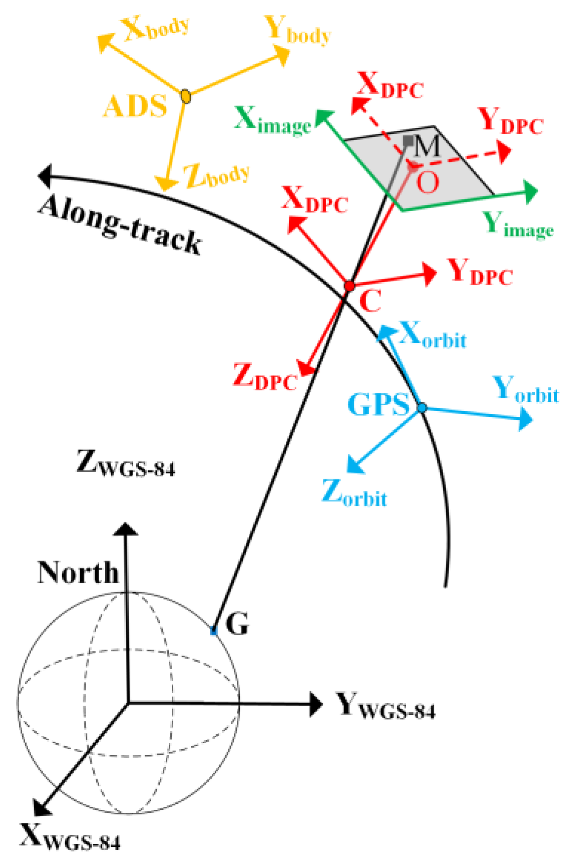
The geometric model of DPC on-orbit imaging is used to describe the geometric mapping relationship between object points in 3D space and image points on the 2D image plane, and it is the basis for DPC on-orbit geolocation and image registration. The geometric model of DPC on-orbit imaging is shown in Figure 2, which involves a series of related coordinate systems, including the image coordinate system, DPC instrument coordinate system, GF-5-02 satellite body coordinate system, orbit coordinate system, and World Geodetic System 1984 (WGS-84). Assuming that the optical system is an ideal optical system, according to the transformation relationship between the coordinate systems and the basic principle of the collinear equation (namely, collinearity of image point M, projection center C, and object point G), the geometric model of DPC on-orbit imaging can be expressed as follows:
where represents the coordinates of object point G in the WGS-84, represents the coordinates of the Global Position System (GPS) phase center in WGS-84, represents the relative deviation between the GPS phase center and DPC projection center C, represents the direction of the incident ray corresponding to the image point M in the DPC instrument coordinate system, and and represent the field angle and azimuth angle of the incident ray, respectively. The corresponding relationship between the direction of incident ray and the coordinates of ideal image points can be described according to the ideal imaging formula of optical system. is the proportionality coefficient, represents the rotation matrix from the orbit coordinate system to WGS-84. ,, is the satellite position at the imaging time , and is the satellite speed at the imaging time , interpolated from GPS data. represents the rotation matrix from GF-5-02 satellite body coordinate system to the orbit coordinate system, represents the attitude parameters of the satellite at the time of imaging, which can be obtained by interpolation of the Attitude Determination System (ADS) data, represents the rotation matrix from the DPC instrument coordinate system to GF-5-02 satellite body coordinate system, and is the installation angle of DPC measured in the laboratory in the GF-5-02 satellite body coordinate system.
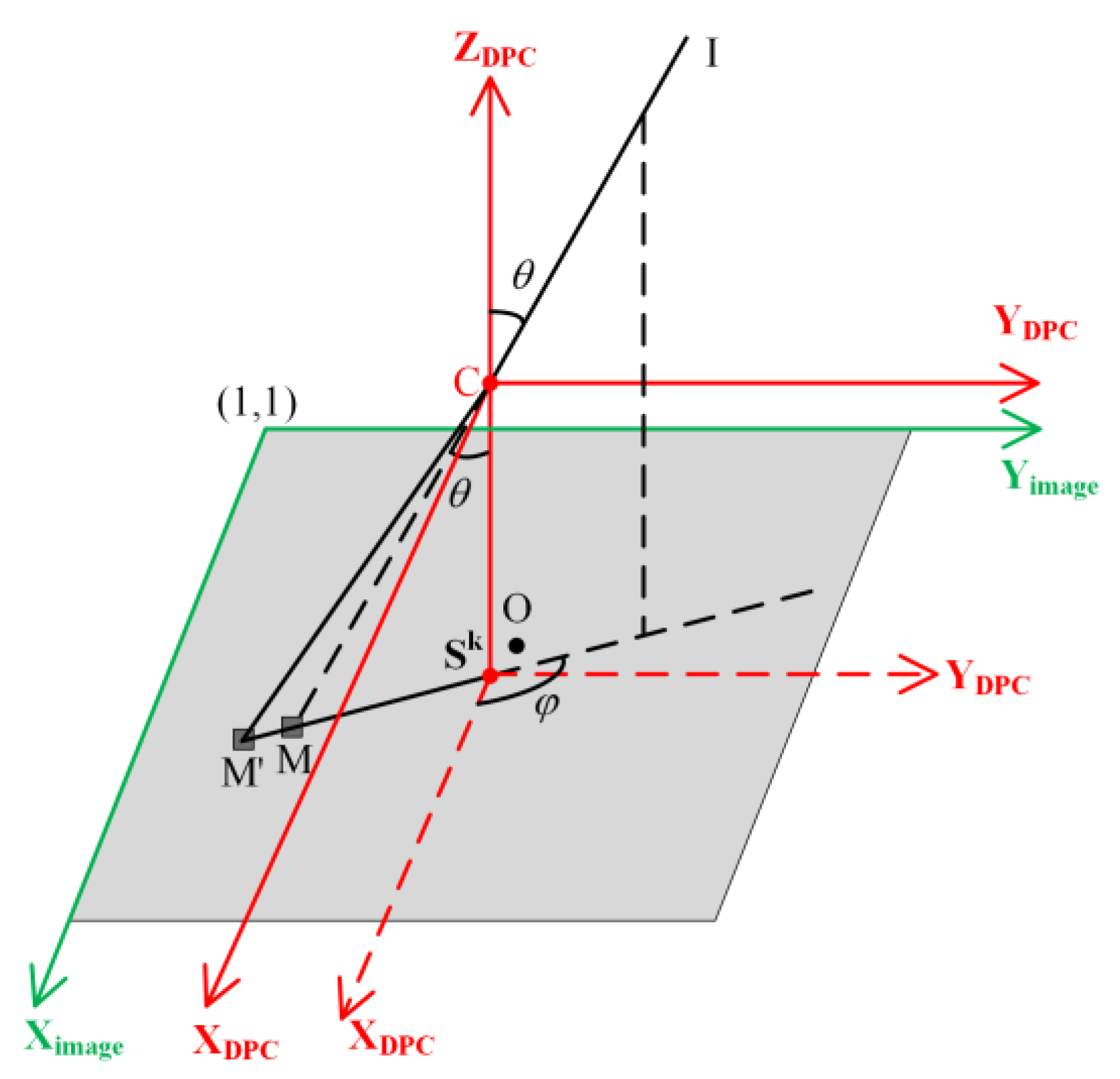
Due to the influence of the distortion of the actual optical system, the actual image point does not coincide with the ideal image point , and the ideal object–image relationship needs to be corrected. Therefore, the laboratory established the corresponding relation between the incident ray direction and the coordinate of the actual image point, as shown in Figure 3.
The actual image point on the CCD imaged by the incident light with the field angle and the azimuth angle is and the imaging process can be described by the following mathematical model:
where is the distortion center of band , denotes the coordinates of the distortion center of band , is the distance between the distortion center and the actual image point , and is the distortion coefficient of the band . In the laboratory, a geometric calibration method based on a separated two-dimensional turntable and the least square optimization theory was used to calibrate the distortion center coordinates and distortion coefficient of each band of DPC [30,31,32].
In the actual projection process, the geometric model of on-orbit imaging composed of Equations (1) and (2) is adopted, combined with the digital elevation model (DEM) and the reference Earth ellipsoid model, to calculate the position of each pixel detection target in the WGS-84 at the imaging time.
According to the physical significance of the parameters of the geometric model of DPC on-orbit imaging, the model parameters can be divided into two categories: the external parameters (installation angle, attitude angle, and projection center position) used to describe the position and attitude of DPC in the WGS-84, and the internal parameters (distortion center and distortion coefficient) used to describe the imaging process of the optical system. To improve the accuracy and efficiency of subsequent on-orbit geometric calibration, it is necessary to further analyze the above two types of model parameters to determine the geometric model parameters to be calibrated.
The installation angle error is a systematic error, including the change in the installation state of the DPC on the satellite platform and the rotation of the CCD. This is due to factors such as vibration during satellite launch and the difference between the on-orbit operating environment and the laboratory environment. The attitude angle error is a random error, which originates from the ADS measurement error (the ADS measurement accuracy is better than ) and the interpolation error caused by the mismatch between the ADS sampling time and the DPC imaging time. The projection center positioning error includes systematic error and random error. The systematic error is the change in the relative position of the projection center and GPS phase center caused by vibration and environmental changes. The random error is caused by GPS orbit measurement error (the orbit measurement accuracy is better than 20 m) and interpolation error caused by the mismatch between GPS sampling time and DPC imaging time. The influence of the projection center positioning error on the geolocation accuracy is equivalent to the error magnitude. It can be ignored for low-resolution instruments such as DPC. Moreover, it can be approximately considered that the projection center of the DPC coincides with the GPS phase center. Equation (1) can, thus, be simplified as follows:
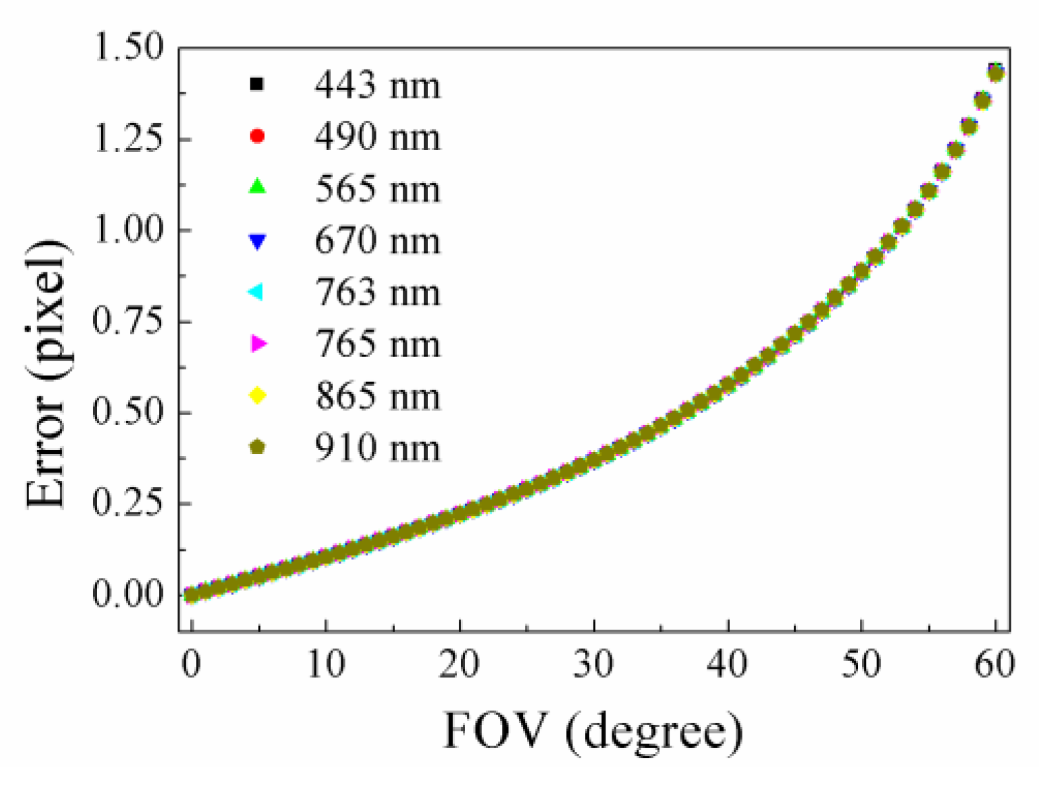
The distortion center error is a systematic error, representing the horizontal offset of the area array CCD and the optical axis, caused by the vibration during the satellite launch and changes in the space environment. The distortion coefficient error is a systematic error caused by the change in the environment of the optical system (such as environmental refractive index, temperature, and other factors). The scaling of CCD pixel size caused by temperature changes can also be described by changes in distortion coefficients. For example, using Zemax analysis, it was found that, when the environment of the DPC optical system is changed from the standard atmosphere to vacuum, the imaging position of the incident beam of the same FOV on the image plane presents an error, as shown in Figure 4. However, the changes in the actual optical system environment are more complicated, and the on-orbit geometric performance of the instrument needs to be determined by on-orbit geometric calibration.
According to the above analysis, after removing the random error term and the error term with a slight influence, the parameters to be calibrated on-orbit include the installation angle of the external parameter and the distortion center and distortion coefficient of the internal parameter. However, it was found that the accuracy of geolocation and image registration is higher when the distortion center remains unchanged. Referring to PARASOL of the same type as DPC, the variation of the distortion center is not considered in its on-orbit geometric calibration [17]. Therefore, the subsequent on-orbit geometric calibration parameters in this paper only include the installation angle in the external parameter and the distortion coefficient in the internal parameter.
3. On-Orbit Autonomous Geometric Calibration Method
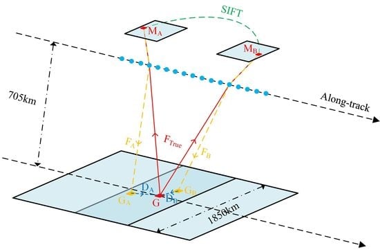
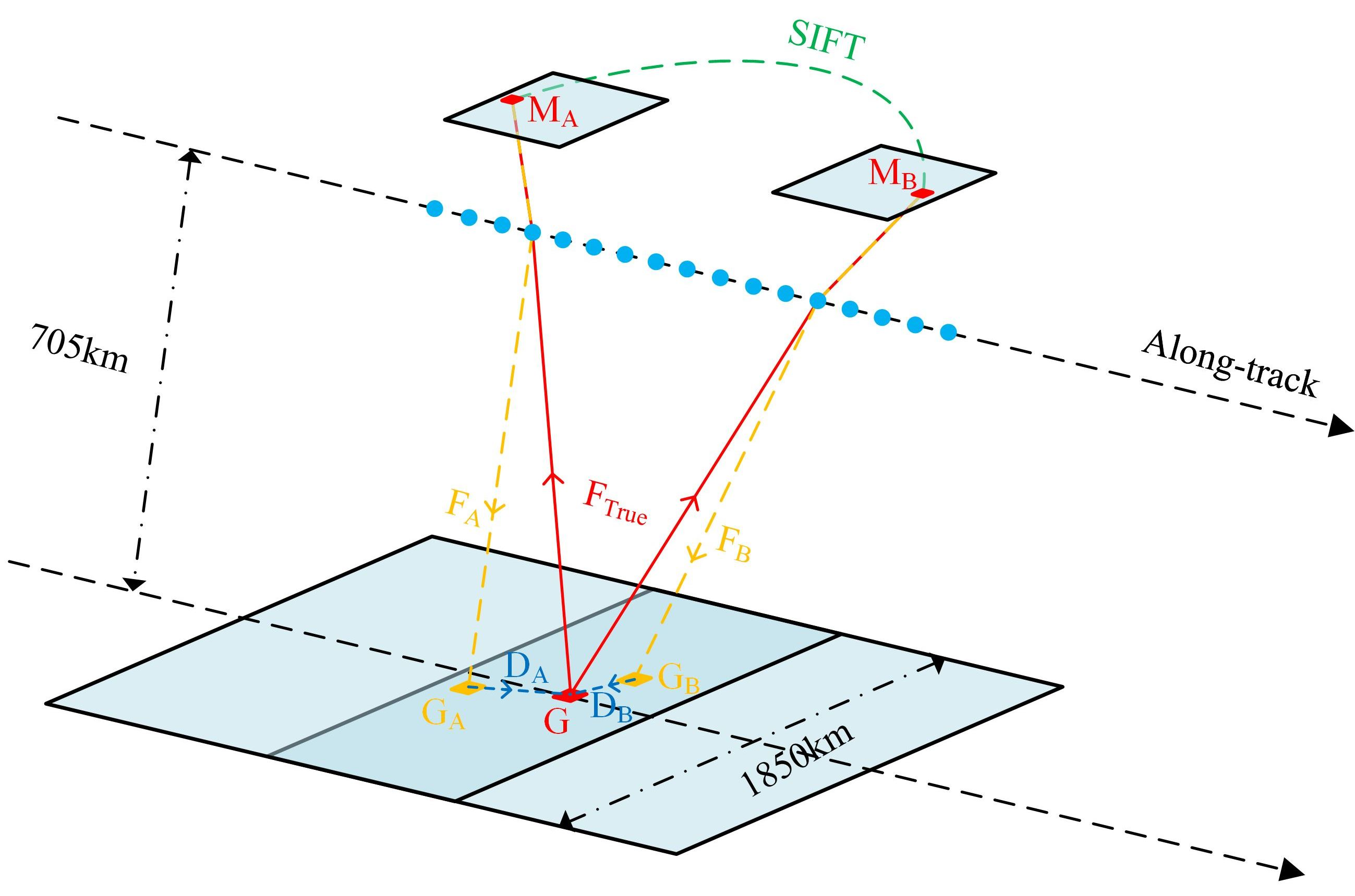
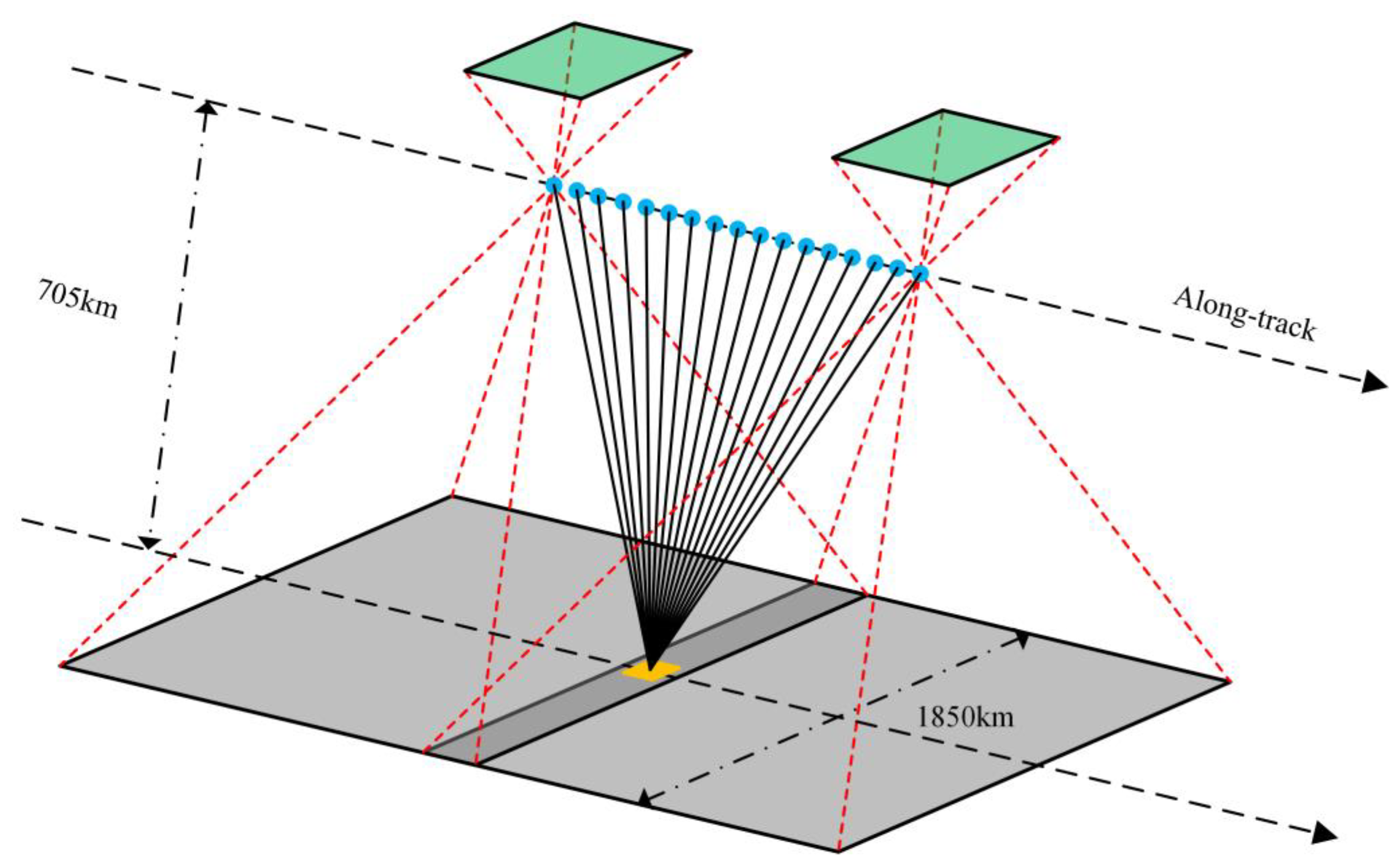
The DPC on-orbit autonomous geometric calibration method benefits from the multiangle observation characteristics of the instrument. The principle of DPC on-orbit multiangle observation is shown in Figure 5. Due to the instrument’s wide FOV imaging capability in the along-track direction, the same ground object can be photographed 17 times in a single satellite transit.
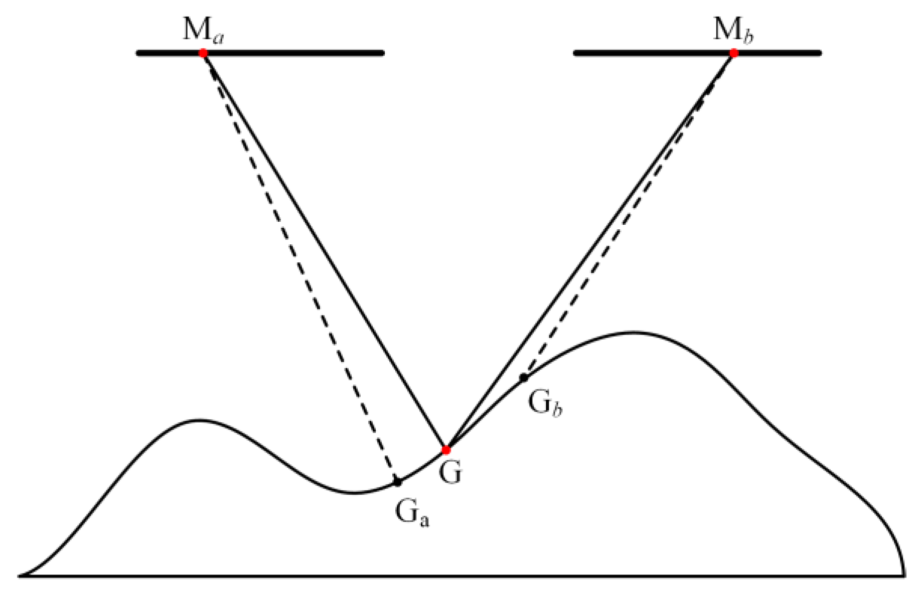
As shown in Figure 6, if the same object G is imaged twice by DPC, the image points are and , respectively. In practice, objects are imaged up to 17 times. When the parameters of the geometric model of DPC on-orbit imaging are ideal and error-free, calculating the coordinates of the target G in the WGS-84 according to the geometric model parameters of the image points and at the imaging time should have the same results. However, the errors in the geometric model parameters often lead to deviations in the calculation results of the target geographic location. The difference between the geolocation result of each image point and the theoretical target point coordinates represents the geolocation error. Differences between homologous point pair geolocation results represent image registration errors.
On the basis of the above analysis, this paper proposes an on-orbit autonomous geometric calibration method that does not require ground calibration field reference data. This method optimizes the geometric model parameters only according to the geometric constraint that homologous points between multiangle images have unique coordinates in WGS-84. The on-orbit autonomous geometric calibration method includes three steps: data preprocessing, multiangle image homologous points matching, and geometric parameter optimization.
- (1)
- Data preprocessing
The data preprocessing stage includes two aspects: preprocessing of the L0-level image data of DPC, and preprocessing of the attitude and orbit parameters. The L0-level image preprocessing includes CCD dark current correction, frame transfer correction, relative response correction, optical system relative response correction, and stray light correction. The attitude and orbit parameter preprocessing needs to analyze the attitude and orbit data from the engineering parameters of the satellite platform, and then obtain the attitude and orbit parameters of each frame of image imaging time according to the imaging time interpolation of DPC.
- (2)
- Homologous point matching
After preprocessing, the scale-invariant feature transform (SIFT) [33,34] algorithm is used to extract feature points in multiangle images. The SIFT algorithm is an image local feature extraction algorithm that finds extreme points as feature points in the Gaussian difference scale space. The feature points extracted by the SIFT algorithm remain invariant to rotation, scaling, and brightness changes, while also maintaining a certain stability to viewing angle changes, affine transformation, and noise. The SIFT algorithm includes four steps of scale space extreme value detection, feature point localization, orientation assignment, and feature point description. After completing the localization and description of the feature points of each angle image, the homologous points between the multiangle images can be matched according to the similarity of the descriptor of the feature points. When matching homologous points, any two of the 17 angle images are paired, with combinations, and then homologous point matching is performed on the two images of each combination. A cloud-free image is selected as best as possible. Because the elevation information of the cloud is unknown, and the cloud is not fixed during multiangle image acquisition, to ensure that there are no cloud pixels at the matched homologous points, cloud pixels need to be removed. In this study, a simple threshold method is adopted to remove cloud pixels. In this method, a reflectivity threshold is set for each band. When the reflectivity of the pixels is higher than this threshold, clouds are identified and removed. Additionally, to eliminate the mismatched points, the random sample consensus (RANSAC) [35] algorithm and the homologous point geographic location constraint threshold are used to eliminate mismatched points. The RANSAC algorithm is an algorithm that removes outliers from a set of sample datasets containing outliers and inliers. The basic principle of using the homologous point geographic location constraint threshold to eliminate mismatched points is that there is no huge deviation when calculating the geographic coordinates of a pair of homologous points using the initial geometric parameters of DPC. Therefore, when the geographic coordinate deviation exceeds a set threshold, it can be regarded as a mismatch. Finally, the homologous point datasets and are formed, as shown in Equation (4). Data points in the two datasets are matched one by one. The information in a single data point includes the coordinates of the image point, attitude, and orbit data at the time of imaging. The precise geographic coordinates of the ground object corresponding to the homologous point are unknown. The on-orbit autonomous geometric calibration method proposed in this paper does not need to know the high-precision geographic coordinate information of these homologous points. This enables the method in this paper to complete the on-orbit autonomous geometric calibration without relying on the reference data of the ground calibration field.
- (3)
- Geometrical parameter optimization
Combined with the geometric model of DPC on-orbit imaging and the geometric constraints of homologous points between multiangle images, the least-squares method can be used to optimize the geometrical parameters to be calibrated. The initial values of the distortion coefficient and installation angle are the results of laboratory calibration tests. The geometrical parameter optimization process can be divided into three steps.
The first step is to use the homologous point data of each band to simultaneously optimize the distortion coefficient and installation angle band by band. The objective equation is shown in Equation (5). In the formula, and correspond to the coordinates of the ground object in WGS-84 calculated from the pair of homologous point data in the datasets and , respectively. The first step optimization results include the distortion coefficient and installation angle of each band.
In the second step, it is considered that all bands should have the same installation angle; however, due to the influence of random errors such as attitude and orbit parameters and the possible correlation between internal and external parameters, the installation angles obtained from each band in the first step are slightly different. Therefore, the average of the installation angles of each band in the first step is taken as the optimization result of the first step. The second step only optimizes the distortion coefficient band by band. The installation angle obtained from the first step is set as the true value. The objective equation of this process is shown in Equation (6). The second step optimization result includes the distortion coefficient of each band.
The third step is to set the distortion coefficient of each band obtained in the second step as the true value and optimize the installation angle band by band. The objective equation of this process is shown in Equation (7). The third step optimization result can be obtained by averaging the installation angles obtained from all band optimizations.
Lastly, when the differences and of two adjacent distortion coefficient optimization results and two adjacent installation angle optimization results are less than the set threshold, the cycle exits, and the on-orbit distortion coefficient and installation angle are output; otherwise, steps 2 and 3 are repeated.
4. Experiment and Discussion
4.1. On-Orbit Geometric Calibration
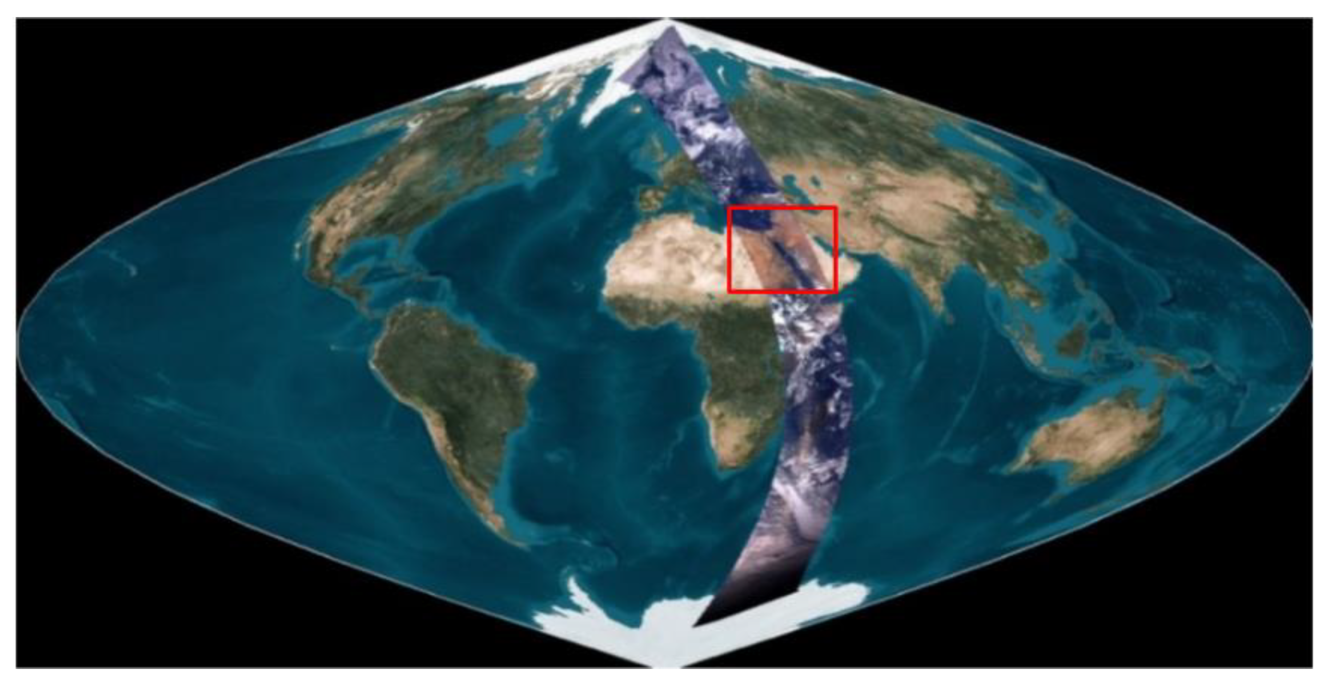
In this paper, the remote sensing images of the Red Sea region taken by DPC on 21 September 2021, are selected for on-orbit geometric calibration, and the corresponding region is shown in the red box in Figure 7. This region is basically cloud-free, and the ground features (surface textures such as coastlines) are relatively wealthy, which is conducive to feature matching to obtain more homologous point pairs and improve the accuracy and stability of on-orbit geometric calibration. In addition, the acquisition time of the calibration image was about 2 weeks after the launch of the satellite, the state of the satellite platform and DPC had stabilized, and the conditions for on-orbit geometric calibration were available.
The DEM reference dataset was GMTED2010 [36], with a spatial resolution of 30 arc seconds, covering most of the world from W to E, S to N, and the global total vertical accuracy was 25–42 m (RMSE). For DPC, an instrument with a nadir spatial resolution of about 1.7 km, along with the resolution and accuracy of the DEM data, could meet the application requirements.
On-orbit initial geometric parameters are provided by laboratory calibration tests. The laboratory calibration test results are shown in Table 2. The laboratory uses a geometric calibration method based on a separated two-dimensional turntable and the least squares optimization theory to calibrate the distortion characteristics of the instrument in a standard atmospheric environment. The calibration results show that the fitting residual between the geometric model and the measured data is better than 0.1 pixel, which confirms the rationality of the geometric model. The laboratory uses the method of prism transfer to measure the installation angle of DPC in the GF-5-02 satellite body coordinate system.
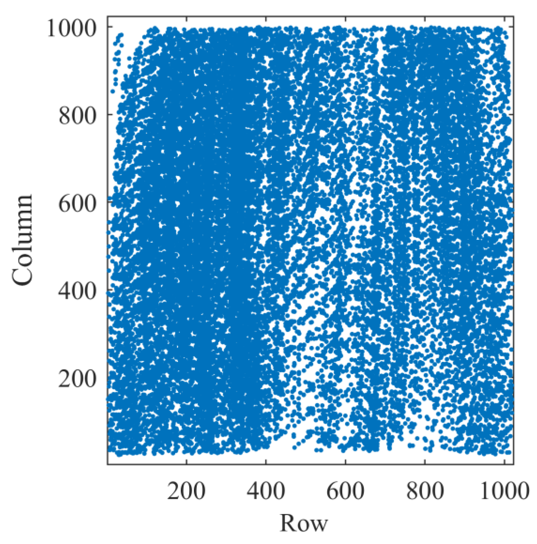
On the basis of the above DEM dataset, laboratory geometric calibration results, the geometric model of DPC on-orbit imaging, and the on-orbit autonomous geometric calibration method proposed in this paper, the geometric parameters are calibrated on-orbit. The on-orbit calibration results are shown in Table 3. By matching multiple groups of images, tens of thousands of homologous point pairs are matched in each band for on-orbit geometric calibration. Among them, the 443 nm band with the least amount of data matched 28,929 homologous point pairs. The distribution of these homologous points on the DPC image plane is shown in Figure 8. It can be seen from the figure that the homologous points were basically evenly distributed on the image plane. This is beneficial for obtaining valid on-orbit geometry parameters. The application of a large amount of data can effectively reduce the influence of random matching error, attitude, and orbit measurement error on the precision of geometric calibration.
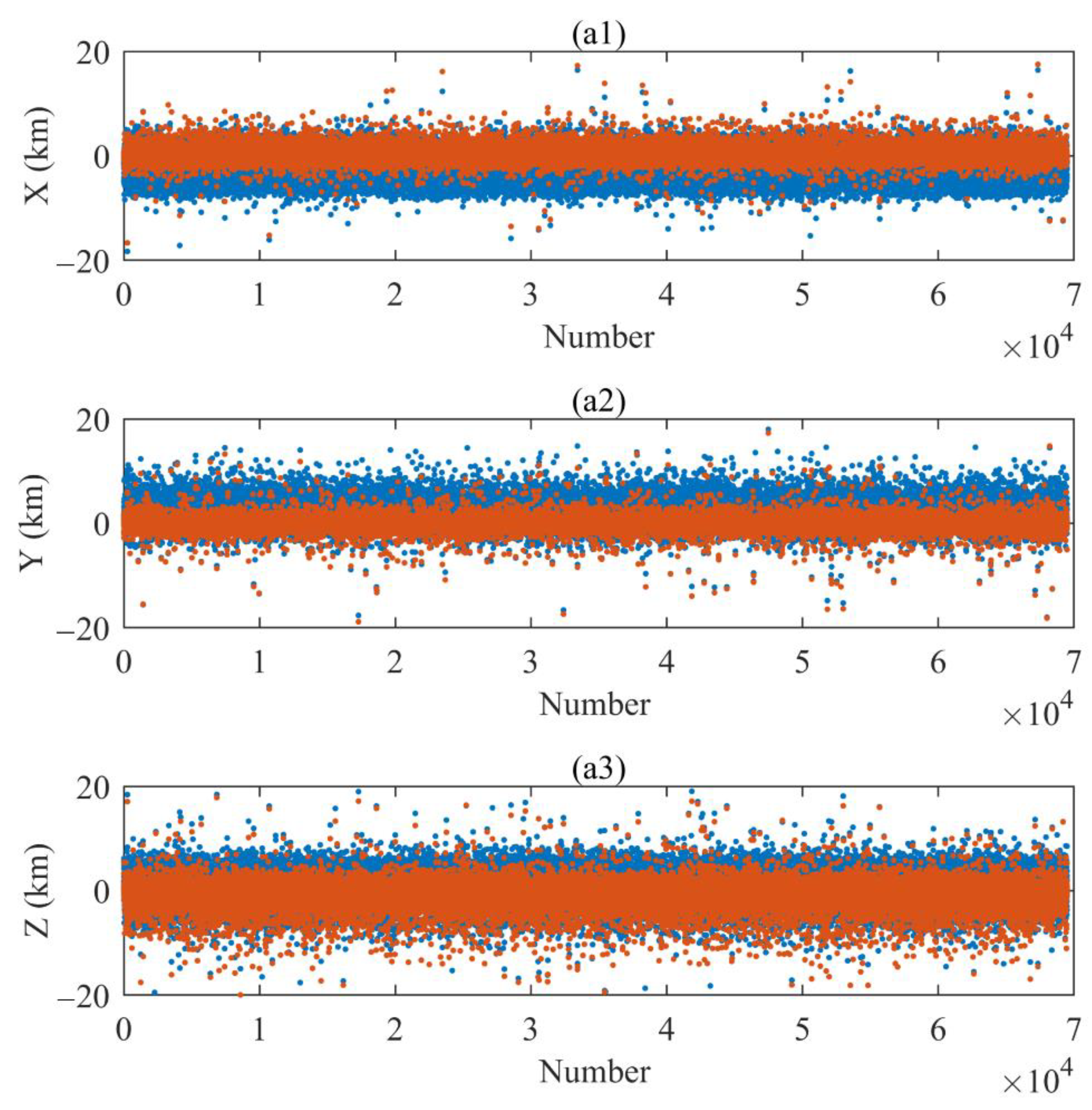
The residual data of the on-orbit geometric calibration in the 670 nm band are shown in Figure 9. The blue points correspond to the initial residuals (obtained using laboratory geometric parameters), and the orange points correspond to the final residuals (obtained using on-orbit geometric parameters). Figure 9a1–a3 correspond to the residuals of the X-, Y-, and Z-coordinates, respectively. The mean values of X, Y, and Z in the initial residual data were −1.459 km, 1.364 km, and 0.567 km, respectively, and the standard deviations (STDs) were 2.054 km, 1.901 km, and 2.501 km, respectively. The mean values of X, Y, and Z in the final residual data were 0.049 km, −0.016 km, −0.140 km, respectively, and the STDs were 0.964 km, 0.861 km, and 1.714 km, respectively. The above results show that, compared with the laboratory geometric parameters, the geometric parameters obtained by the on-orbit autonomous geometric calibration method in this paper were more consistent with the actual on-orbit data, which proves the effectiveness of the method in this paper.
4.2. Relative Geolocation Accuracy Evaluation
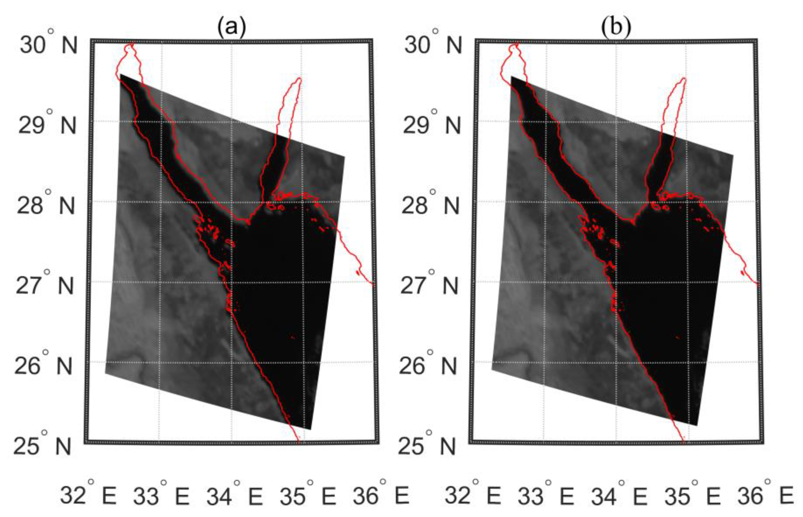
To verify the validity of the on-orbit autonomous geometric calibration method. In this paper, the GSHHG [37] coastline data were used as a reference to evaluate the relative geolocation accuracy before and after DPC on-orbit geometric calibration. Two sets of geometric parameters before and after the on-orbit geometric calibration were used to project the original image. Taking the 910 nm band as an example, the results are shown in Figure 10. Figure 10a,b represent the matching relationship between the local area projection results of the original image and the reference coastline before and after the on-orbit geometric calibration, respectively. The results shown in Figure 10 correspond to the original resolution (nadir resolution 1.7 km) of the DPC without merging pixels. The results show that the DPC projection results after the on-orbit autonomous geometric calibration were significantly more consistent with the reference coastline data, which can preliminarily prove the effectiveness of the on-orbit autonomous geometric calibration method in this paper.
In order to further quantitatively analyze the impact of on-orbit geometric calibration on the geolocation accuracy of DPC, the coastline crossing method (CCM) [38,39,40] was used for quantitative evaluation. The CCM was originally developed for the Earth Radiation Budget Experiment (ERBE) scanner [38]. The basic idea of this method is that there is a significant difference in brightness temperature between the sea surface and land; hence, there is a large gradient change at the junction of sea and land. The subpixel location of the coastline can be achieved by fitting a cubic polynomial to the brightness temperature of four consecutive pixels (along the row or column direction) near the coastline. The cubic polynomial form is as follows:
where represents the brightness temperature of pixel , and represents the longitude or latitude of pixel . is a polynomial coefficient with the solution shown as follows:
After the polynomial coefficients are known, the inflection point position can be calculated. When is between and , and is greater than the set threshold, the inflection point represents the coastline. Finally, the coastline data located by the CCM is matched with the reference coastline data, and the outliers are eliminated. The deviation between the two represents the relative geolocation error of the instrument.
In this paper, an improved CCM is proposed. The method first uses the Canny [41] operator for pixel-level edge localization, and then uses the polynomial fitting method of the original CCM for subpixel localization. After calculating the position of the subpixel inflection point, if it is located in the pixel where the Canny operator initially locates the edge, and is greater than the set threshold, then the inflection point is considered the coastline. The method first uses the Canny operator to initially locate the pixel-level edge, which can quickly identify the potential coastline position, eliminate a large amount of invalid data, locate the subpixel-level coastline position more quickly, and improve the algorithm efficiency.
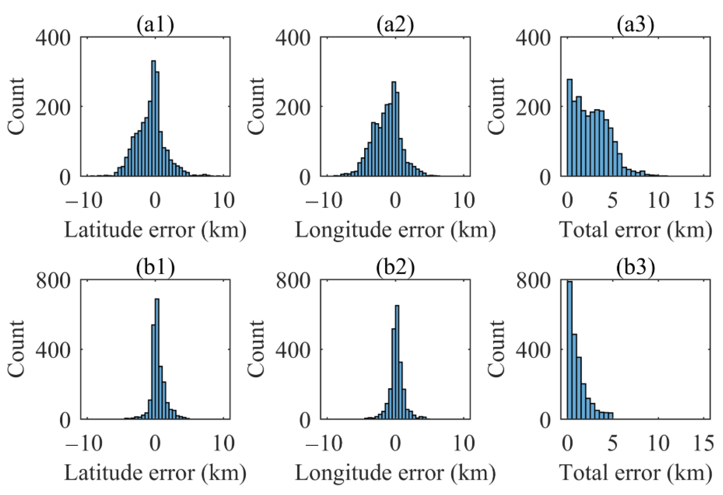
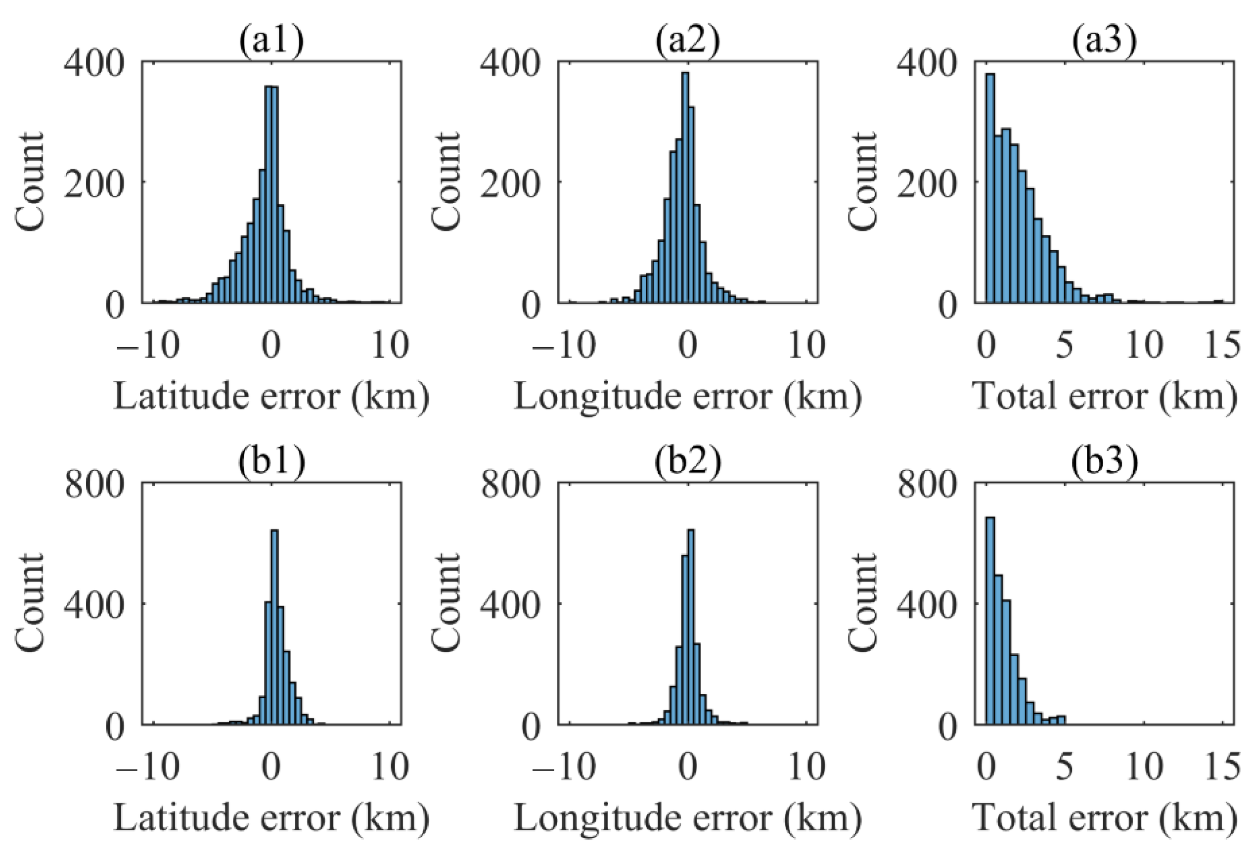
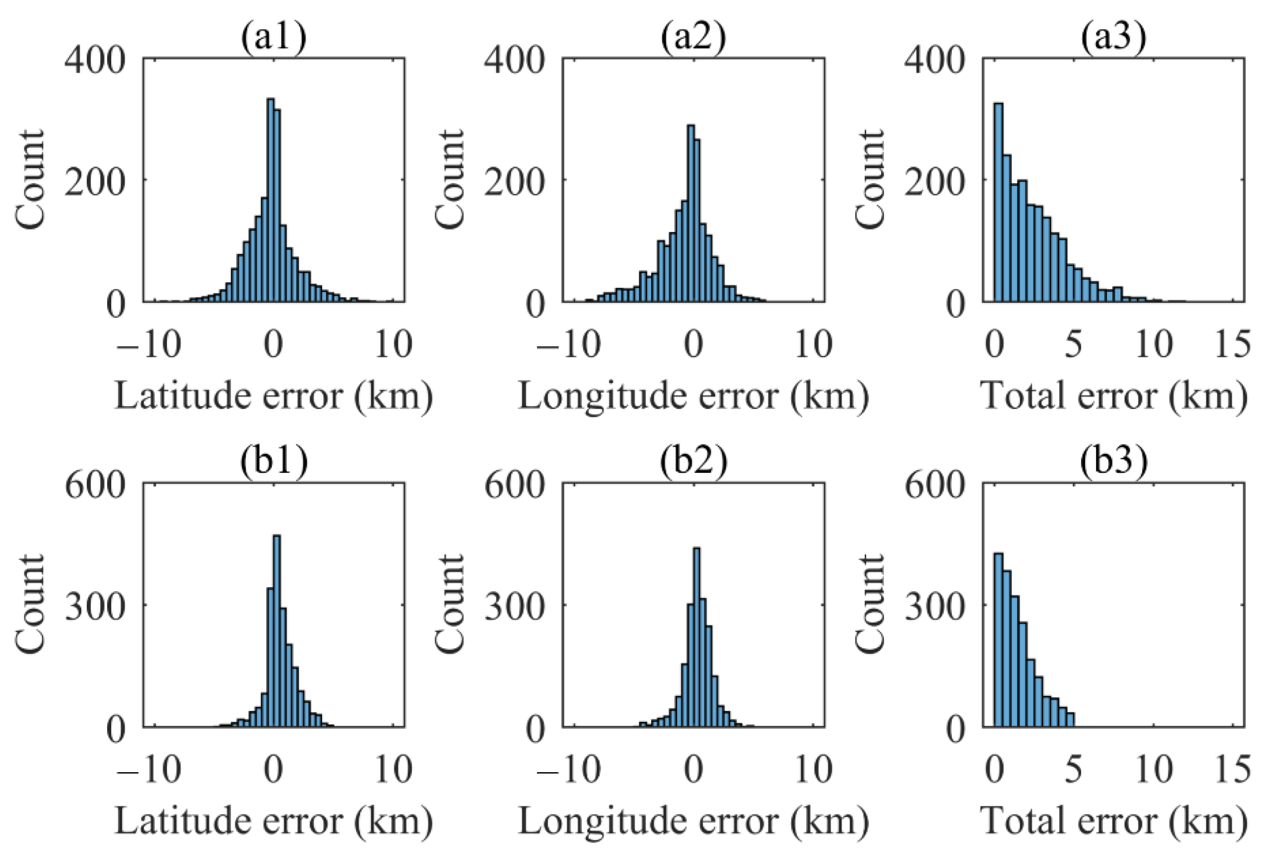
The improved CCM was used to evaluate the relative geolocation accuracy of the DPC, taking the 910 nm band as an example. To fully verify the improvement effect of the on-orbit autonomous geometric calibration method on the relative geolocation accuracy, three sets of completely independent DPC data were used to evaluate the relative geolocation accuracy. One of the sets of data was the orbit 202 data acquired on 21 September 2021, which is the same as the data used for on-orbit geometric calibration. The additional two datasets were acquired on 19 September 2021 and 23 September 2021, corresponding to orbits 173 and 231. In the short term, the geometric performance of DPC could remain stable. The relative geolocation evaluation results of the three groups of data before and after the on-orbit geometric calibration are shown in Figure 11, Figure 12 and Figure 13, respectively, where (a1), (a2), and (a3) represent the latitude error, longitude error, and total error between the coastline geolocation by DPC before on-orbit geometric calibration and the reference coastline, respectively, while (b1), (b2), (b3) are the results after on-orbit geometric calibration. Figure 11, Figure 12 and Figure 13 contain 2209, 2150, and 1902 statistical data points, respectively. All three sets of validation data show that on-orbit geometric calibration significantly improved the on-orbit relative geolocation accuracy of DPC. The error in the longitude direction, the error in the latitude direction, and the total error were significantly improved after geometric calibration. The mean and STD of the data in the histogram were calculated, and the results are shown in Table 4. The relative geolocation evaluation results of the three sets of data were basically the same. Among the three sets of results, the maximum mean value of the total error before the on-orbit geometric calibration was about 2.725 km, with the maximum STD of 2.238 km. After on-orbit geometric calibration, the maximum mean value of the total error was about 1.275 km, with the maximum STD of 1.157 km.
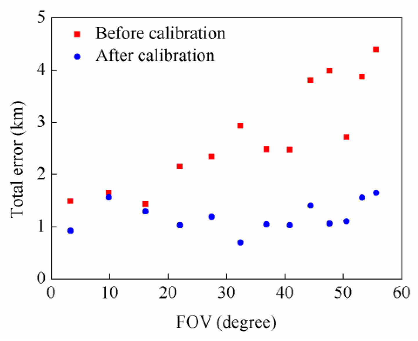
Additionally, the FOV correlation of the aforesaid total error data was analyzed by taking the orbit 202 data as an example, and the relationship between the error mean and the FOV is shown in Figure 14. The results show that the relative geolocation error increased with the increasing FOV before the on-orbit geometric calibration, but the relative geolocation accuracy remained the same with the increase in FOV after the on-orbit geometric calibration. This further demonstrates the effectiveness of the proposed method in improving the relative geolocation accuracy of DPC on-orbit.
4.3. Image Registration Accuracy Evaluation
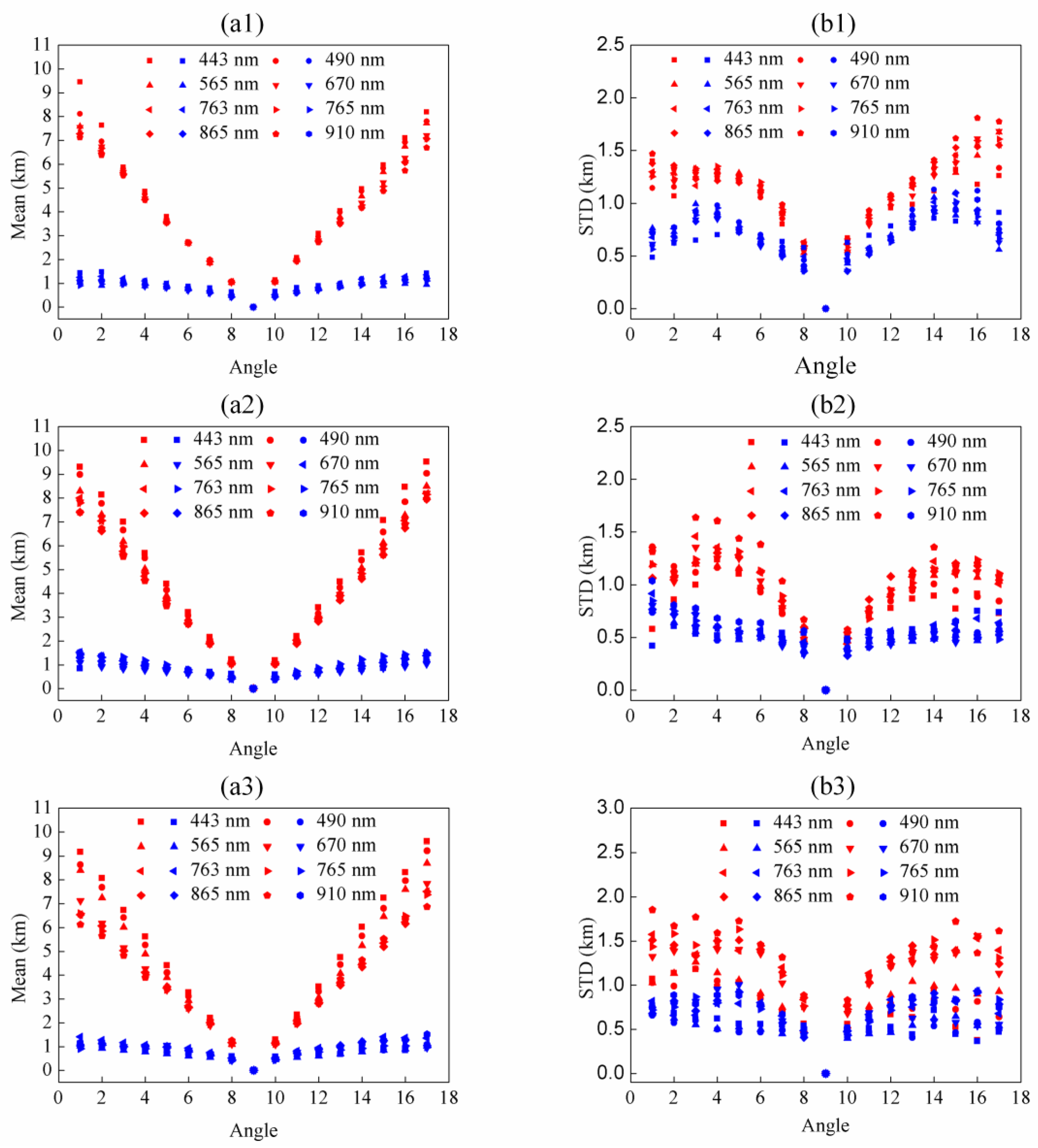
The performance of DPC on-orbit image registration was evaluated using the SIFT algorithm, including multiangle image registration and multispectral image registration. The data used to evaluate the image registration performance are consistent with the data used for the relative geolocation accuracy assessment. In the evaluation of multi-angle image registration performance, this paper took the ninth angle image of each band as the reference image to evaluate the registration accuracy of the remaining 16 angle images relative to the reference image. The reason is that the images of the ninth angle and the other 16 angles have a relatively large overlap area, which is conducive to matching more feature points and avoids the inability to accurately evaluate the multiangle image registration performance due to insufficient feature points. The evaluation results of each band are shown in Figure 15. Figure 15a1,b1 correspond to the mean and STD of the orbit 202 evaluation results. Figure 15a2,b2 correspond to the mean and STD of the orbit 173 evaluation results. Figure 15a3,b3 correspond to the mean and STD of the orbit 231 evaluation results. Red represents before the on-orbit geometric calibration, while blue represents after the on-orbit geometric calibration. All three sets of results show that the on-orbit geometric calibration could effectively improve the multiangle registration accuracy of DPC, especially when the angle number difference is large. Furthermore, the on-orbit geometric calibration could greatly improve the consistency of the registration performance between each angle image and the reference image. The short-wave bands (443 nm, 490 nm) are greatly affected by aerosols; hence, there are certain differences in the STD of the short-wave bands in the three sets of data results. Among the three sets of results, the maximum mean and STD of the multiangle registration error before on-orbit geometric calibration were about 9.607 km and 1.852 km respectively. The maximum mean and STD after on-orbit geometric calibration were 1.530 km and 1.130 km, respectively. Considering that the ground sampling distance (GSD) corresponding to the DPC L1-level data grid was 3.3 km, the mean and STD of the above registration errors were 2.911 GSD, 0.562 GSD, 0.464 GSD, and 0.342 GSD, respectively, when the GSD was taken as the unit.
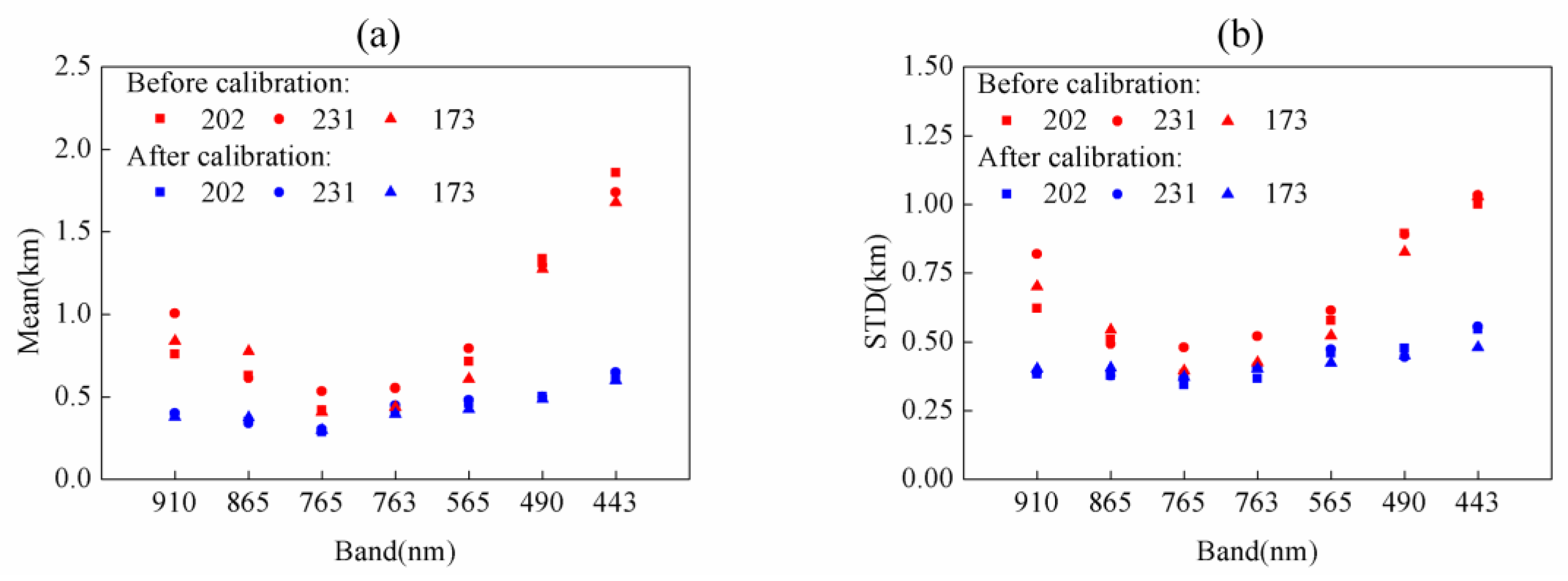
The multispectral image registration performance evaluation took the 670 nm band as the reference band and evaluated the registration accuracy of other bands relative to the reference band. The 670 nm band was used as a reference mainly because the imaging time of this band is in the middle of an imaging cycle of DPC, and there is a large overlap area with the data of each band. The 670 nm band is less affected by aerosols, and there is no effect of gas absorption. The results are shown in Figure 16. Figure 16a,b respectively represent the mean and STD. After the geometric calibration, the multispectral image registration performance was significantly improved, and the consistency of the registration performance of all bands was also improved. The evaluation results of the three sets of data were basically the same. Among the three sets of results, before the on-orbit geometric calibration, the maximum mean and maximum STD of multispectral image registration errors were about 1.859 km (0.563 GSD) and 1.033 km (0.313 GSD), respectively. After the on-orbit geometric calibration, they were 0.650 km (0.197 GSD) and 0.555 km (0.168 GSD), respectively. However, the registration accuracy of the 443 nm band and 490 nm band relative to the reference band was relatively low both before and after geometric calibration. The reason is that the signals of these two bands were relatively weak, the signal-to-noise ratio was low, and the atmospheric radiation signal was strong, which led to the blurring of the surface feature information. Therefore, the matching error of the SIFT algorithm increased when the algorithm was used for matching, which led to the registration performance declining to a certain extent compared with other bands.
5. Conclusions
In this paper, an on-orbit autonomous geometric calibration method was proposed, which does not require reference data from the ground calibration field. The on-orbit autonomous geometric calibration method is based on the multiangle imaging characteristics of DPC, and the geometric model parameters are optimized by the geometric constraints of the homologous points between the multiangle images. Using this method, the installation angle and the instrument distortion coefficient in the geometric model of DPC are calibrated on-orbit. To verify the effectiveness of this method, the DPC relative geolocation accuracy and image registration performance were compared and verified. The evaluation method of on-orbit relative geolocation accuracy is based on the improved CCM, and the reference coastline data are GSHHG. The SIFT algorithm was used to evaluate the image registration performance, including multiangle image registration performance and multispectral image registration performance. The results demonstrate that the proposed on-orbit autonomous geometric calibration method could effectively improve the accuracy of DPC relative geolocation and image registration. It is proven that this method could realize the on-orbit autonomous geometric calibration of spaceborne optical instruments without the ground calibration field. However, there were still some errors in relative geolocation and image registration after geometric calibration on-orbit, which may be from the following aspects: (1) the deviation between the geometric model of DPC on-orbit imaging and the actual model; (2) measurement error and interpolation error of attitude and orbit data; (3) error of coastline subpixel positioning algorithm; (4) image registration algorithm error; (5) influence of the accuracy of the on-orbit autonomous geometric calibration method itself. Therefore, to further improve the accuracy of DPC on-orbit relative geolocation and image registration, it is necessary to further study the above problems. Additionally, it is necessary to further evaluate and analyze the long-term variation characteristics of DPC geometric model parameters, image registration performance, and relative geolocation accuracy.
Author Contributions
Conceptualization, G.X. and B.M.; methodology, G.X. and B.M.; software, G.X.; validation, G.X. and B.M.; formal analysis, G.X.; investigation, G.X. and B.M.; resources, G.X., B.T. and B.M.; data curation, G.X., X.L., T.S. and B.T.; writing—original draft preparation, G.X.; writing—review and editing, G.X., L.H. and B.M.; visualization, G.X.; supervision, B.M. and J.H.; project administration, D.L. and J.H.; funding acquisition, D.L. and J.H. All authors have read and agreed to the published version of the manuscript.
Funding
This research was funded by the K. C. Wong Education Foundation “International team of Advanced Polarization Remote Sensing Technology and Application” (GJTD-2018-15).
Data Availability Statement
Not applicable.
Acknowledgments
We thank the DPC team for their contributions to the project and the manuscript.
Conflicts of Interest
The authors declare no conflict of interest.
References
- Liu, Y.; Sun, D.; Hu, X.; Ye, X.; Li, Y.; Liu, S.; Cao, K.; Chai, M.; Zhou, W.; Zhang, J.; et al. The Advanced Hyperspectral Imager: Aboard China’s GaoFen-5 Satellite. IEEE Trans. Geosci. Remote Sens. 2019, 7, 23–32. [Google Scholar] [CrossRef]
- Zhao, Y.; Li, Y. Technical Characteristics and Application of Visible and Infrared Multispectral Imager. In Proceedings of the 6th International Symposium of Space Optical Instruments and Applications, Delft, The Netherlands, 24–25 September 2021; Space Technology Proceedings. Urbach, H.P., Yu, Q., Eds.; Springer International Publishing: Cham, Switzerland, 2021; Volume 7, pp. 197–208. [Google Scholar]
- Shi, H.; Li, Z.; Ye, H.; Luo, H.; Xiong, W.; Wang, X. First Level 1 Product Results of the Greenhouse Gas Monitoring Instrument on the GaoFen-5 Satellite. IEEE Trans. Geosci. Remote Sens. 2021, 59, 899–914. [Google Scholar] [CrossRef]
- Zhao, M.; Si, F.; Zhou, H.; Jiang, Y.; Ji, C.; Wang, S.; Zhan, K.; Liu, W. Pre-Launch Radiometric Characterization of EMI-2 on the GaoFen-5 Series of Satellites. Remote Sens. 2021, 13, 2843. [Google Scholar] [CrossRef]
- Dubovik, O.; Li, Z.; Mishchenko, M.I.; Tanré, D.; Karol, Y.; Bojkov, B.; Cairns, B.; Diner, D.J.; Espinosa, W.R.; Goloub, P.; et al. Polarimetric remote sensing of atmospheric aerosols: Instruments, methodologies, results, and perspectives. J. Quant. Spectrosc. Radiat. Transf. 2019, 224, 474–511. [Google Scholar] [CrossRef]
- Huang, C.; Chang, Y.; Xiang, G.; Han, L.; Chen, F.; Luo, D.; Li, S.; Sun, L.; Tu, B.; Meng, B.; et al. Polarization measurement accuracy analysis and improvement methods for the directional polarimetric camera. Opt. Express 2020, 28, 38638–38666. [Google Scholar] [CrossRef]
- Huang, C.; Xiang, G.; Chang, Y.; Han, L.; Zhang, M.; Li, S.; Tu, B.; Meng, B.; Hong, J. Pre-flight calibration of a multi-angle polarimetric satellite sensor directional polarimetric camera. Opt. Express 2020, 28, 13187–13215. [Google Scholar] [CrossRef]
- Yao, P.; Tu, B.; Xu, S.; Yu, X.; Xu, Z.; Luo, D.; Hong, J. Non-uniformity calibration method of space-borne area CCD for directional polarimetric camera. Opt. Express 2021, 29, 3309–3326. [Google Scholar] [CrossRef]
- Huang, C.; Zhang, M.; Chang, Y.; Chen, F.; Han, L.; Meng, B.; Hong, J.; Luo, D.; Li, S.; Sun, L.; et al. Directional polarimetric camera stray light analysis and correction. Appl. Opt. 2019, 58, 7042–7049. [Google Scholar] [CrossRef]
- Shi, E.; Wang, Y.; Jia, N.; Mao, J.; Lu, G.; Liang, S. Absorbing Aerosol Sensor on Gao-Fen 5B satellite. Adv. Opt. Technol. 2018, 7, 387–393. [Google Scholar] [CrossRef]
- Shang, H.; Letu, H.; Chen, L.; Riedi, J.; Ma, R.; Wei, L.; Labonnote, L.C.; Hioki, S.; Liu, C.; Wang, Z.; et al. Cloud thermodynamic phase detection using a directional polarimetric camera (DPC). J. Quant. Spectrosc. Radiat. Transf. 2020, 253, 107179. [Google Scholar] [CrossRef]
- Li, Z.; Hou, W.; Hong, J.; Zheng, F.; Luo, D.; Wang, J.; Gu, X.; Qiao, Y. Directional Polarimetric Camera (DPC): Monitoring aerosol spectral optical properties over land from satellite observation. J. Quant. Spectrosc. Radiat. Transf. 2018, 218, 21–37. [Google Scholar] [CrossRef]
- Yu, H.; Ma, J.; Ahmad, S.; Sun, E.; Li, C.; Li, Z.; Hong, J. Three-Dimensional Cloud Structure Reconstruction from the Directional Polarimetric Camera. Remote Sens. 2019, 11, 2894. [Google Scholar] [CrossRef]
- Durieux, A.; Neubert, S.; Petitbon, I. POLDER: A wide field-of-view instrument for earth-polarized observation. Proc. SPIE 1994, 2209, 160–169. [Google Scholar]
- Bret-Dibat, T.; Andre, Y.; Laherrere, J.M. Preflight calibration of the POLDER instrument. Proc. SPIE 1995, 2553, 218–231. [Google Scholar]
- Hagolle, O.; Guerry, A.; Cunin, L.; Millet, B.; Perbos, J.; Laherrere, J.M.; Bret-Dibat, T.; Poutier, L. POLDER level-1 processing algorithms. Proc. SPIE 1996, 2758, 308–319. [Google Scholar]
- Fougnie, B.; Bracco, G.; Lafrance, B.; Ruffel, C.; Hagolle, O.; Tinel, C. PARASOL in-flight calibration and performance. Appl. Opt. 2007, 46, 5435–5451. [Google Scholar] [CrossRef]
- Fougnie, B.; Marbach, T.; Lacan, A.; Lang, R.; Schlüssel, P.; Poli, G.; Munro, R.; Couto, A.B. The multi-viewing multi-channel multi-polarisation imager—Overview of the 3MI polarimetric mission for aerosol and cloud characterization. J. Quant. Spectrosc. Radiat. Transf. 2018, 219, 23–32. [Google Scholar] [CrossRef]
- Wang, M.; Tian, Y.; Cheng, Y. Development of On-orbit Geometric Calibration for High Resolution Optical Remote Sensing Satellite. Geo. Spat. Inf. Sci. 2017, 42, 1580–1588. [Google Scholar]
- Wang, M.; Yang, B.; Hu, F.; Zang, X. On-Orbit Geometric Calibration Model and Its Applications for High-Resolution Optical Satellite Imagery. Remote Sens. 2014, 6, 4391–4408. [Google Scholar] [CrossRef]
- Zhang, Z.; Tang, Q. Camera Self-Calibration Based on Multiple View Images. In Proceedings of the 2016 Nicograph International (NicoInt), Hanzhou, China, 6–8 July 2016; pp. 88–91. [Google Scholar]
- Hemayed, E.E. A survey of camera self-calibration. In Proceedings of the IEEE Conference on Advanced Video and Signal Based Surveillance, Miami, FL, USA, 21–22 July 2003; pp. 351–357. [Google Scholar]
- Malis, E.; Cipolla, R. Camera self-calibration from unknown planar structures enforcing the multiview constraints between collineations. IEEE Trans. Pattern Anal. Mach. Intell. 2002, 24, 1268–1272. [Google Scholar] [CrossRef]
- Yilmaztürk, F. Full-automatic self-calibration of color digital cameras using color targets. Opt. Express 2011, 19, 18164–18174. [Google Scholar] [CrossRef] [PubMed]
- Greslou, D.; Lussy, F.D.; Delvit, J.M.; Dechoz, C.; Amberg, V. Pleiades-HR innovative techniques for geometric image quality commissioning. ISPRS Int. Arch. Photogramm. Remote Sens. Spatial Inf. Sci. 2012, XXXIX-B1, 543–547. [Google Scholar] [CrossRef]
- Wang, M.; Cheng, Y.; Tian, Y.; He, L.; Wang, Y. A New On-Orbit Geometric Self-Calibration Approach for the High-Resolution Geostationary Optical Satellite GaoFen4. IEEE J. Sel. Top. Appl. Earth Obs. Remote Sens. 2018, 11, 1670–1683. [Google Scholar] [CrossRef]
- Zhang, G.; Xu, K.; Zhang, Q.; Li, D. Correction of Pushbroom Satellite Imagery Interior Distortions Independent of Ground Control Points. Remote Sens. 2018, 10, 98. [Google Scholar] [CrossRef] [Green Version]
- Zhang, G.; Deng, M.; Cai, C.; Zhao, R. Geometric Self-Calibration of YaoGan-13 Images Using Multiple Overlapping Images. Sensors 2019, 19, 2367. [Google Scholar] [CrossRef]
- Gleyzes, M.A.; Perret, L.; Kubik, P. Pleiades system architecture and main performances. ISPRS Int. Arch. Photogramm. Remote Sens. Spatial Inf. Sci. 2012, XXXIX-B1, 537–542. [Google Scholar]
- Chen, L.; Zheng, X.; Hong, J.; Qiao, Y.; Wang, Y. A novel method for adjusting CCD camera in geometrical calibration based on a two-dimensional turntable. Optik 2010, 121, 486–489. [Google Scholar] [CrossRef]
- Huang, C.; Chang, Y.; Han, L.; Wu, S.; Li, S.; Luo, D.; Sun, L.; Hong, J. Geometric calibration method based on Euler transformation for a large field of view polarimetric imager. J. Mod. Opt. 2020, 67, 1524–1533. [Google Scholar] [CrossRef]
- Huang, C.; Meng, B.; Chang, Y.; Chen, F.; Zhang, M.; Han, L.; Xiang, G.; Tu, B.; Hong, J. Geometric calibration method based on a two-dimensional turntable for a directional polarimetric camera. Appl. Opt. 2020, 59, 226–233. [Google Scholar] [CrossRef]
- Lowe, D.G. Distinctive image features from scale-invariant keypoints. Int. J. Comput. Vis. 2004, 60, 91–110. [Google Scholar] [CrossRef]
- Lowe, D.G. Object recognition from local scale-invariant features. In Proceedings of the Seventh IEEE International Conference on Computer Vision, Kerkyra, Greece, 20–27 September 1999; pp. 1150–1157. [Google Scholar]
- Fischler, M.A.; Bolles, R.C. Random Sample Consensus: A Paradigm for Model Fitting with Applications to Image Analysis and Automated Cartography. Commun. ACM 1981, 24, 381–395. [Google Scholar] [CrossRef]
- Jeffrey, J.D.; Dean, B.G. Global Multi-Resolution Terrain Elevation Data 2010 (GMTED2010). U.S. Geological Survey Open-File Report 2011–1073. Available online: https://pubs.er.usgs.gov/publication/ofr20111073 (accessed on 23 April 2022).
- Wessel, P.; Smith, W.H.F. A global self-consistent, hierarchical, high resolution shoreline database. J. Geophys. Res. Solid Earth 1996, 101, 7989–8743. [Google Scholar] [CrossRef]
- Hoffman, L.F.; Weaver, W.L.; Kibler, J.F. Calculation and Accuracy of ERBE Scanner Measurement Locations. NASA Technical Paper 2670; NASA Langley Research Center: Hampton, VA, USA, 1981. [Google Scholar]
- Han, Y.; Weng, F.; Zou, X.; Yang, H.; Scott, D. Characterization of geolocation accuracy of Suomi NPP Advanced Technology Microwave Sounder measurements. J. Geophys. Res. Atmos. 2016, 121, 4933–4950. [Google Scholar] [CrossRef]
- Tang, F.; Zou, X.; Yang, H.; Weng, F. Estimation and Correction of Geolocation Errors in FengYun-3C Microwave Radiation Imager Data. IEEE Trans. Geosci. Remote Sens. 2016, 54, 407–420. [Google Scholar] [CrossRef]
- Canny, J. A Computational Approach to Edge Detection. IEEE Trans. Pattern Anal. Mach. Intell. 1986, 8, 679–698. [Google Scholar] [CrossRef]
Figure 1.
Optical structure of DPC.

Figure 2.
Geometric model of DPC on-orbit imaging.

Figure 3.
Object-image geometric relationship of DPC.

Figure 4.
DPC geometric performance environmental difference analysis results.

Figure 5.
On-orbit multiangle observation principle of DPC.

Figure 6.
Schematic diagram of geolocation and registration error of DPC.

Figure 7.
L1-level data preview of DPC. Corresponding to orbit 202.

Figure 8.
Distribution of homologous points in the 443 nm band.

Figure 9.
Residual comparison before and after calibration at 670 nm. The blue points correspond to the initial residuals, and the orange points correspond to the final residuals. Subgraphs (a1), (a2), and (a3) correspond to the residuals of the X-, Y-, and Z-coordinates, respectively.
Figure 9.
Residual comparison before and after calibration at 670 nm. The blue points correspond to the initial residuals, and the orange points correspond to the final residuals. Subgraphs (a1), (a2), and (a3) correspond to the residuals of the X-, Y-, and Z-coordinates, respectively.

Figure 10.
Result of coastline comparison, with no pixels merged, corresponding to the original resolution of the image: (a) before the on-orbit geometric calibration; (b) after the on-orbit geometric calibration.
Figure 10.
Result of coastline comparison, with no pixels merged, corresponding to the original resolution of the image: (a) before the on-orbit geometric calibration; (b) after the on-orbit geometric calibration.

Figure 11.
On-orbit relative geolocation accuracy results for DPC, corresponding to orbit 202: (a1–a3) before the on-orbit geometric calibration; (b1–b3) after the on-orbit geometric calibration.
Figure 11.
On-orbit relative geolocation accuracy results for DPC, corresponding to orbit 202: (a1–a3) before the on-orbit geometric calibration; (b1–b3) after the on-orbit geometric calibration.

Figure 12.
On-orbit relative geolocation accuracy results for DPC, corresponding to orbit 173: (a1–a3) before the on-orbit geometric calibration; (b1–b3) after the on-orbit geometric calibration.
Figure 12.
On-orbit relative geolocation accuracy results for DPC, corresponding to orbit 173: (a1–a3) before the on-orbit geometric calibration; (b1–b3) after the on-orbit geometric calibration.

Figure 13.
On-orbit relative geolocation accuracy results for DPC, corresponding to orbit 231: (a1–a3) before the on-orbit geometric calibration; (b1–b3) after the on-orbit geometric calibration.
Figure 13.
On-orbit relative geolocation accuracy results for DPC, corresponding to orbit 231: (a1–a3) before the on-orbit geometric calibration; (b1–b3) after the on-orbit geometric calibration.

Figure 14.
FOV correlation analysis of DPC relative geolocation accuracy. Red represents before the on-orbit geometric calibration, while blue represents after the on-orbit geometric calibration.
Figure 14.
FOV correlation analysis of DPC relative geolocation accuracy. Red represents before the on-orbit geometric calibration, while blue represents after the on-orbit geometric calibration.

Figure 15.
On-orbit multi-angle image registration performance of DPC. Red represents before the on-orbit geometric calibration, while blue represents after the on-orbit geometric calibration: (a1,b1) corresponding to orbit 202; (a2,b2) corresponding to orbit 173; (a3,b3) corresponding to orbit 231.

Figure 16.
On-orbit multi-spectral image registration performance of DPC. Red represents before the on-orbit geometric calibration, while blue represents after the on-orbit geometric calibration. Subgraphs (a,b) represent the mean and STD of multi-spectral image registration performance, respectively.


Table 1.
DPC parameters.
| Parameter | GF-5-01 | GF-5-02 | DQ-1 | CM | |
|---|---|---|---|---|---|
| Focal length (mm) | 4.83 | 5.54 | 5.54 | 4.83 | |
| FOV (degree) | Along-track | ±50 | ±50 | ±50 | ±50 |
| Cross-track | ±50 | ±50 | ±50 | ±40 | |
| Relative aperture | 1:4 | 1:4.26 | 1:4.26 | 1:4 | |
| CCD array size | 512 × 512 | 1024 × 1024 | 1024 × 1024 | 360 × 512 | |
| Pixel size (μm) | 22.5 × 22.5 | 13 × 13 | 13 × 13 | 22.5 × 22.5 | |
| Orbit altitude (km) | 705 | 705 | 705 | 505 | |
| Band (nm) | Polarized | 490 (20) 670 (20) 865(40) | |||
| Nonpolarized | 443 (20) 565 (20) 763 (10) 765 (40) 910(20) | ||||
| Swath (km) | Along-track | 1850 | 1850 | 1850 | 1250 |
| Cross-track | 1850 | 1850 | 1850 | 850 | |
| Observation angle | 9 | 17 | 17 | 9 | |
| Nadir resolution (km) | 3.3 | 1.7 | 1.7 | 2.5 | |
Table 2.
Results of laboratory geometric calibration.
| Parameter | 443 nm | 490 nm | 565 nm | 670 nm | 763 nm | 765 nm | 865 nm | 910 nm |
|---|---|---|---|---|---|---|---|---|
| (pixel) | 512.055 | 512.073 | 512.025 | 512.047 | 512.044 | 511.985 | 512.041 | 512.058 |
| (pixel) | 519.338 | 519.334 | 519.308 | 519.321 | 517.297 | 519.312 | 519.318 | 519.354 |
| (pixel) | 434.884 | 433.724 | 432.767 | 432.092 | 431.743 | 431.758 | 431.494 | 431.425 |
| (pixel) | 1.776 | 2.869 | 3.995 | 5.139 | 5.838 | 5.768 | 6.415 | 6.533 |
| (pixel) | −1.646 | −2.261 | −2.903 | −3.600 | −4.026 | −3.940 | −4.393 | −4.422 |
| (pixel) | −0.731 | −0.629 | −0.519 | −0.378 | −0.291 | −0.333 | −0.209 | −0.228 |
| (pixel) | 0.246 | 0.242 | 0.238 | 0.230 | 0.224 | 0.231 | 0.217 | 0.223 |
| (degree) | −0.001 | |||||||
| (degree) | 0.022 | |||||||
| (degree) | −0.058 | |||||||
Table 3.
Results of on-orbit autonomous geometric calibration.
| Parameter | 443 nm | 490 nm | 565 nm | 670 nm | 763 nm | 765 nm | 865 nm | 910 nm |
|---|---|---|---|---|---|---|---|---|
| (pixel) | 512.055 | 512.073 | 512.025 | 512.047 | 512.044 | 511.985 | 512.041 | 512.058 |
| (pixel) | 519.338 | 519.334 | 519.308 | 519.321 | 517.297 | 519.312 | 519.318 | 519.354 |
| (pixel) | 430.671 | 429.612 | 428.661 | 428.306 | 428.137 | 427.899 | 427.824 | 427.861 |
| (pixel) | 0.112 | 2.297 | 3.977 | 5.330 | 6.269 | 6.363 | 6.912 | 6.668 |
| (pixel) | 2.745 | 0.282 | −0.762 | −1.692 | −2.146 | −2.214 | −2.444 | −1.944 |
| (pixel) | −2.876 | −1.632 | −1.334 | −1.082 | −1.069 | −1.001 | −1.001 | −1.285 |
| (pixel) | 0.650 | 0.416 | 0.376 | 0.351 | 0.370 | 0.349 | 0.359 | 0.409 |
| (degree) | 0.047 | |||||||
| (degree) | −0.024 | |||||||
| (degree) | 0.219 | |||||||
Table 4.
On-orbit relative geolocation accuracy results for DPC.
| Stage | No. | Mean (km) | STD (km) | ||||
|---|---|---|---|---|---|---|---|
| Latitude | Longitude | Total | Latitude | Longitude | Total | ||
| Before | 202 | −0.720 | −1.291 | 2.725 | 2.120 | 2.088 | 1.902 |
| 173 | −0.593 | −0.645 | 2.221 | 2.231 | 2.050 | 2.238 | |
| 231 | −0.247 | −0.805 | 2.443 | 2.062 | 2.258 | 2.022 | |
| After | 202 | 0.386 | 0.175 | 1.131 | 1.050 | 1.076 | 1.076 |
| 173 | 0.461 | 0.019 | 1.192 | 1.015 | 0.971 | 0.966 | |
| 231 | 0.555 | 0.308 | 1.275 | 1.270 | 1.225 | 1.157 | |
Publisher’s Note: MDPI stays neutral with regard to jurisdictional claims in published maps and institutional affiliations. |
© 2022 by the authors. Licensee MDPI, Basel, Switzerland. This article is an open access article distributed under the terms and conditions of the Creative Commons Attribution (CC BY) license (https://creativecommons.org/licenses/by/4.0/).
Share and Cite
MDPI and ACS Style
Xiang, G.; Meng, B.; Tu, B.; Lei, X.; Sheng, T.; Han, L.; Luo, D.; Hong, J. On-Orbit Autonomous Geometric Calibration of Directional Polarimetric Camera. Remote Sens. 2022, 14, 4548. https://doi.org/10.3390/rs14184548
AMA Style
Xiang G, Meng B, Tu B, Lei X, Sheng T, Han L, Luo D, Hong J. On-Orbit Autonomous Geometric Calibration of Directional Polarimetric Camera. Remote Sensing. 2022; 14(18):4548. https://doi.org/10.3390/rs14184548
Chicago/Turabian StyleXiang, Guangfeng, Binghuan Meng, Bihai Tu, Xuefeng Lei, Tingrui Sheng, Lin Han, Donggen Luo, and Jin Hong. 2022. "On-Orbit Autonomous Geometric Calibration of Directional Polarimetric Camera" Remote Sensing 14, no. 18: 4548. https://doi.org/10.3390/rs14184548
Note that from the first issue of 2016, this journal uses article numbers instead of page numbers. See further details here.