


Horticultural Image Feature Matching Algorithm Based on Improved ORB and LK Optical Flow

Abstract
:
1. Introduction
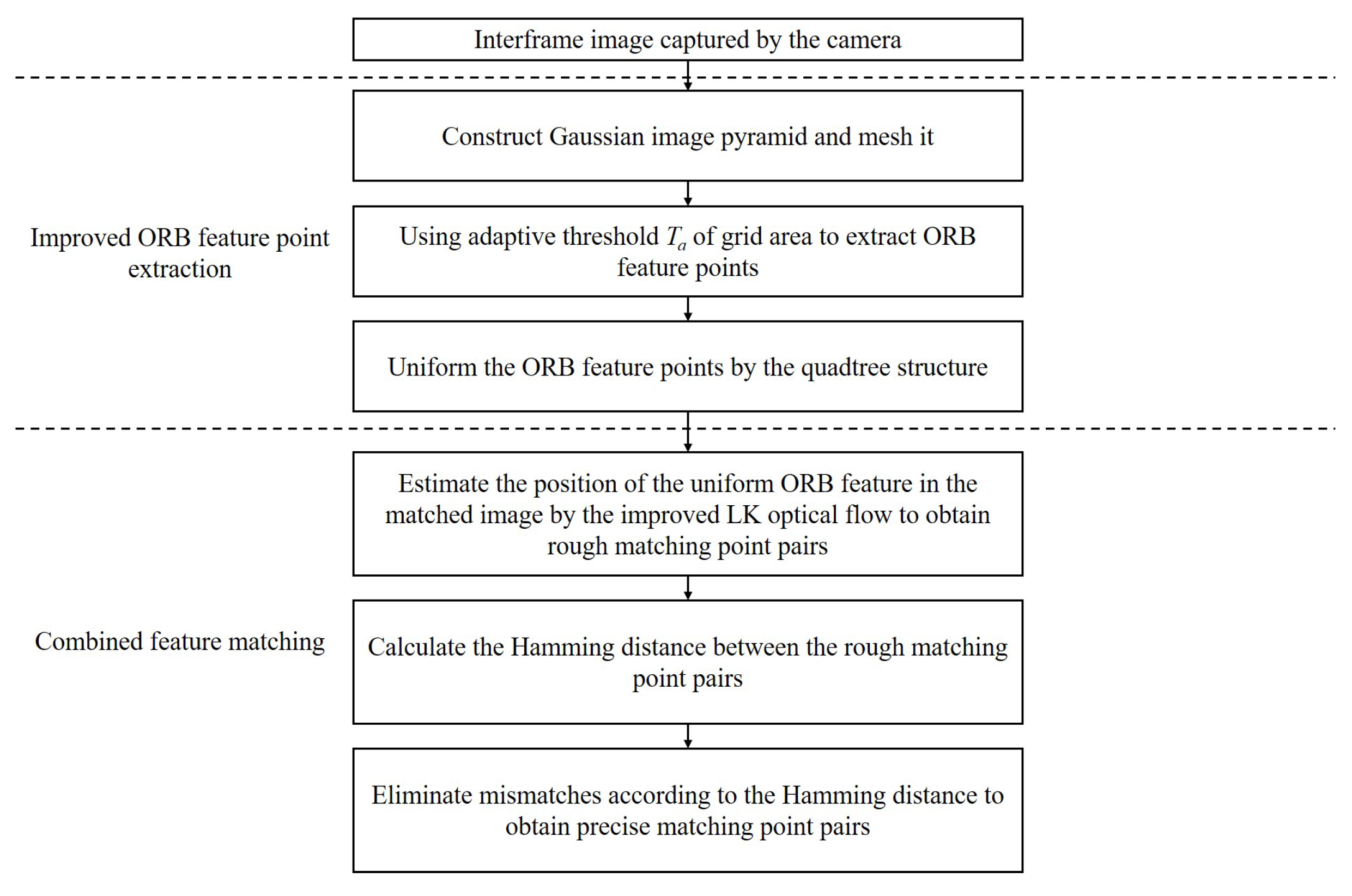
2. Methodology
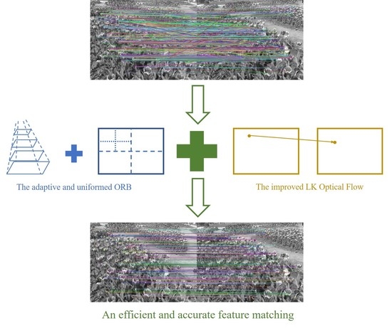
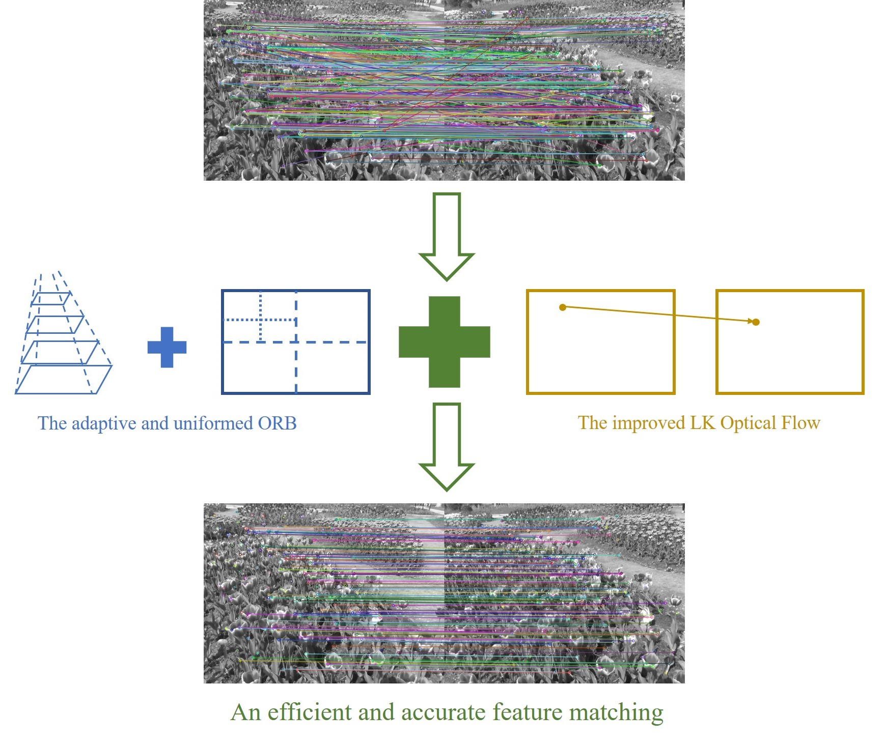
2.1. Algorithm Framework
2.2. Improved ORB Feature Point Extraction
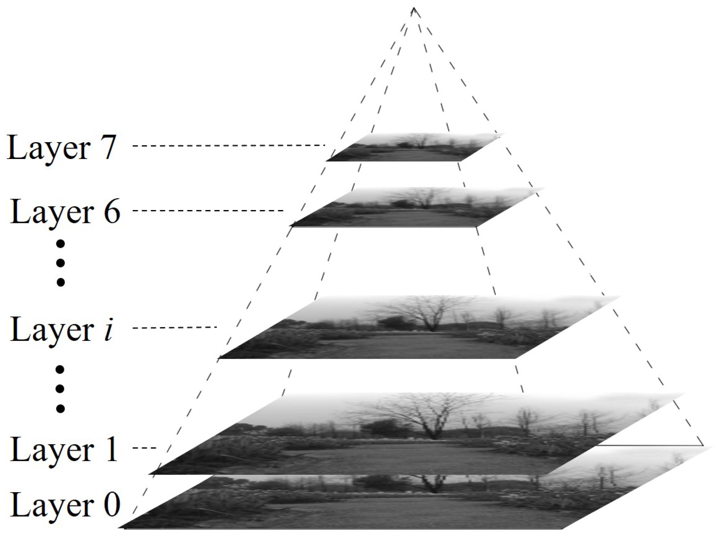
2.2.1. Construct Gaussian Image Pyramid
2.2.2. Adaptive Threshold Based on the Mesh Region
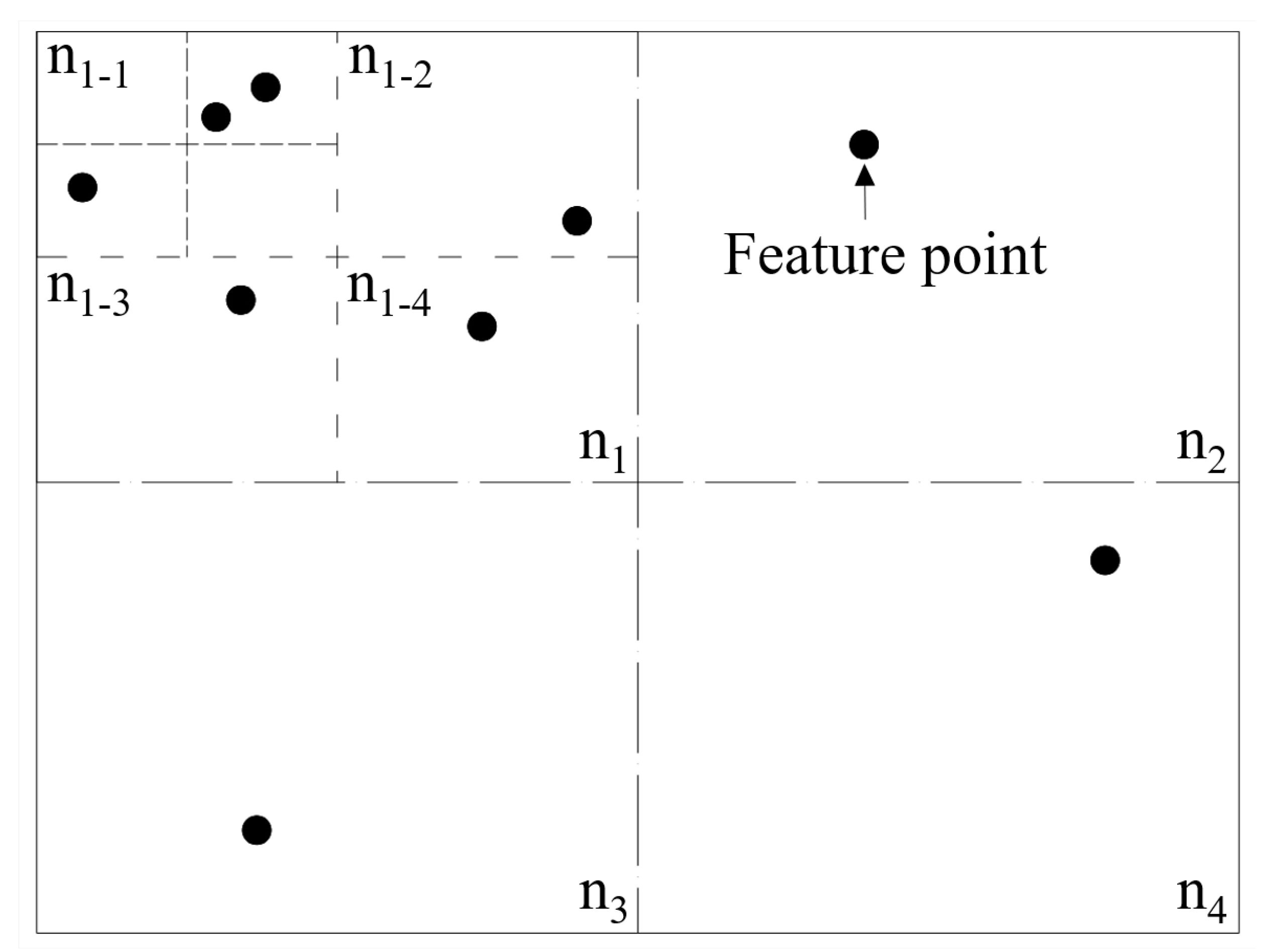
2.2.3. Uniform Feature Points Based on Quadtree
2.3. Combined Feature Matching
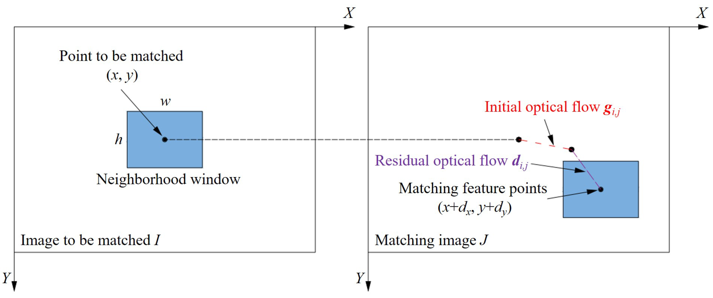
2.3.1. Improved LK Optical Flow Method
2.3.2. Feature Rough Matching Based on Improved ORB-LK Optical Flow
2.3.3. Feature Precise Matching Based on Feature Descriptor
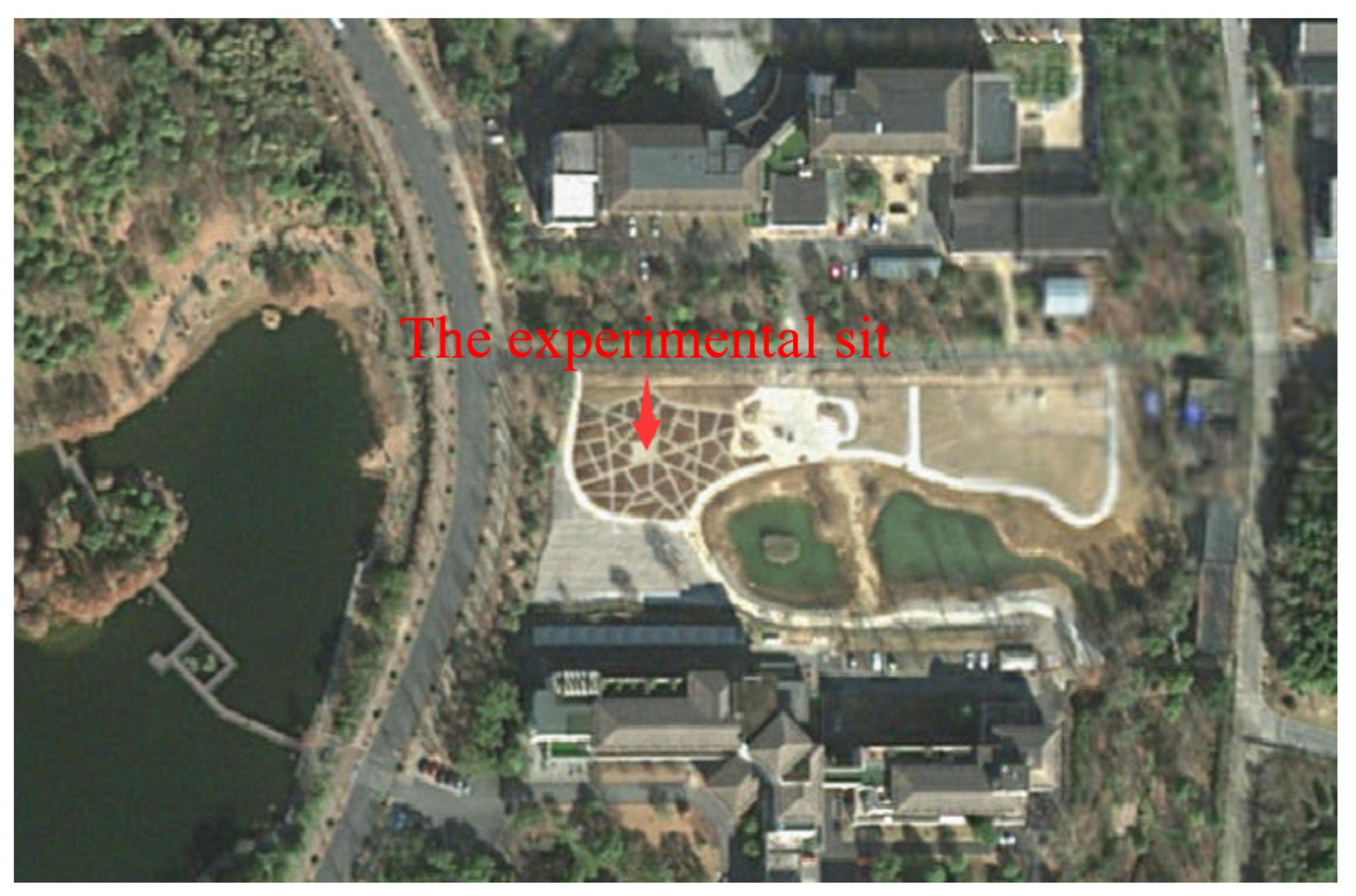
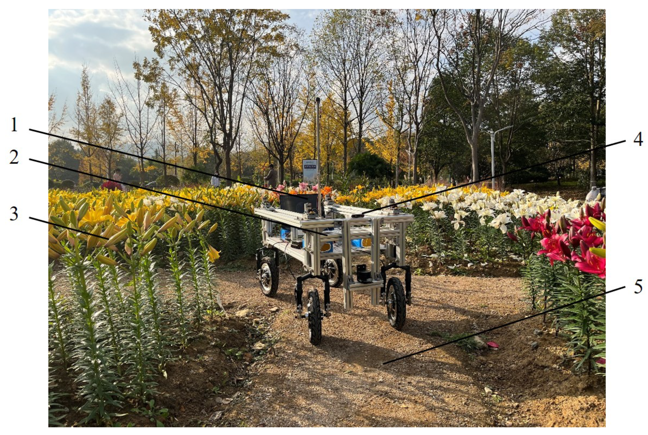
3. Experimental Results and Discussion
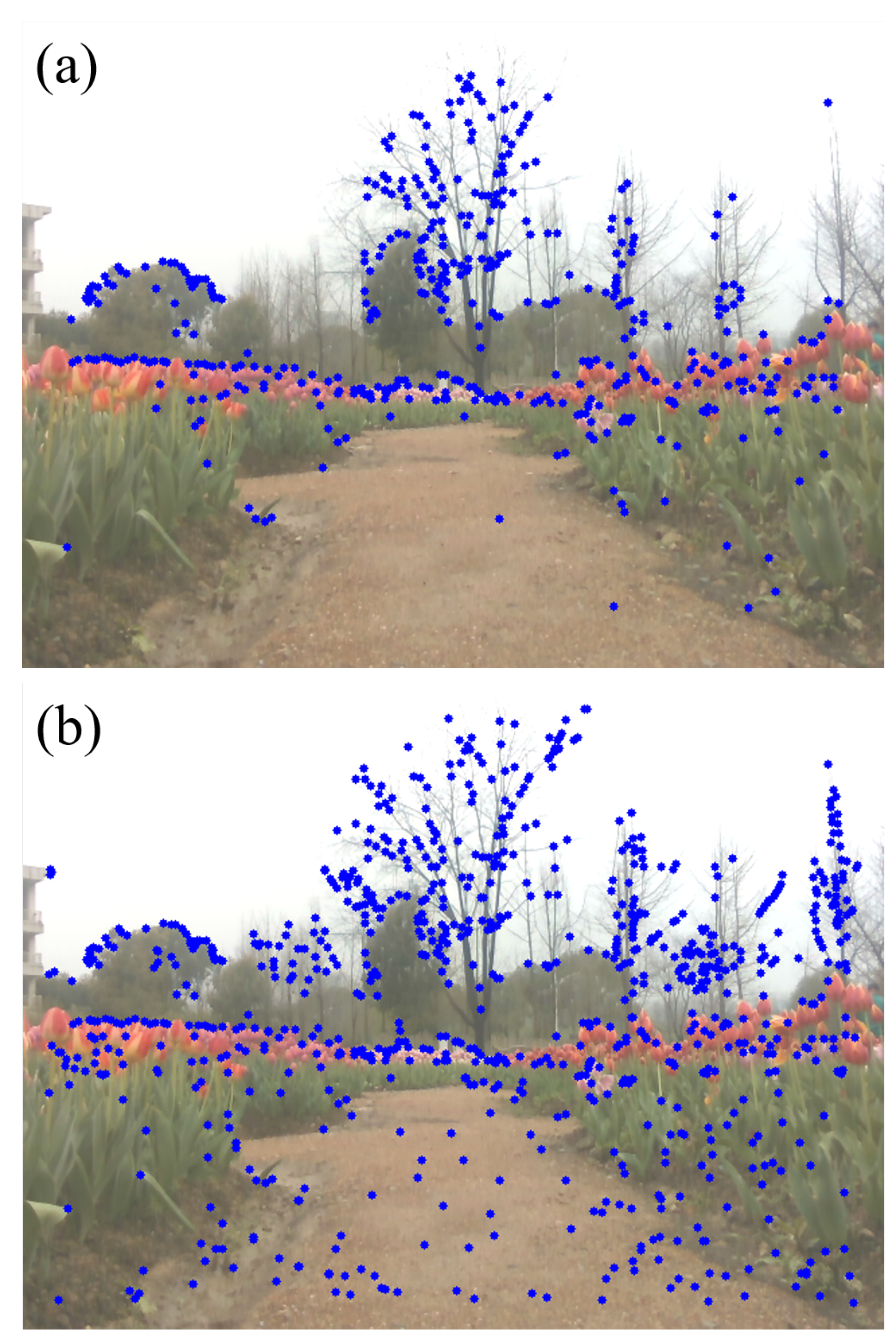
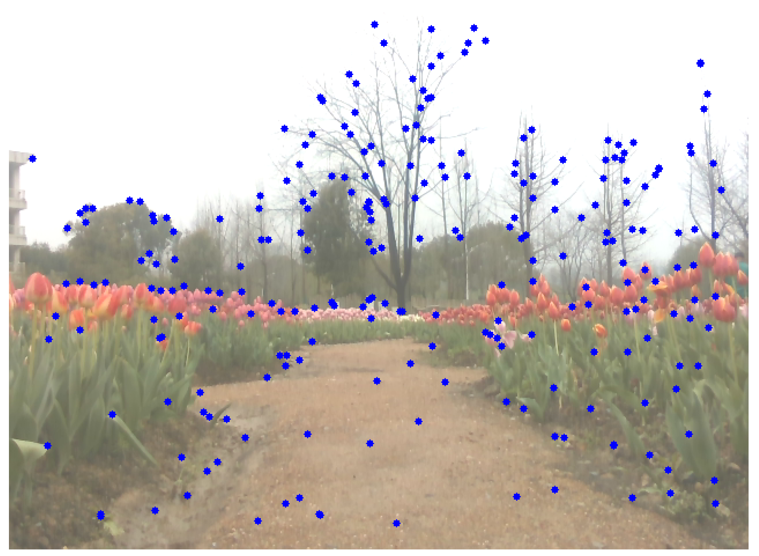
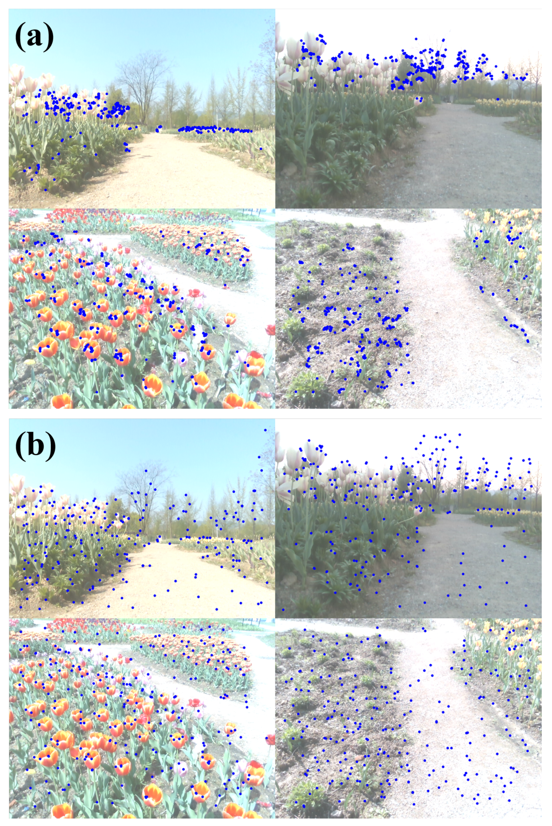
3.1. Quality and Analysis of Feature Point Extraction
3.1.1. Results
3.1.2. Discussion
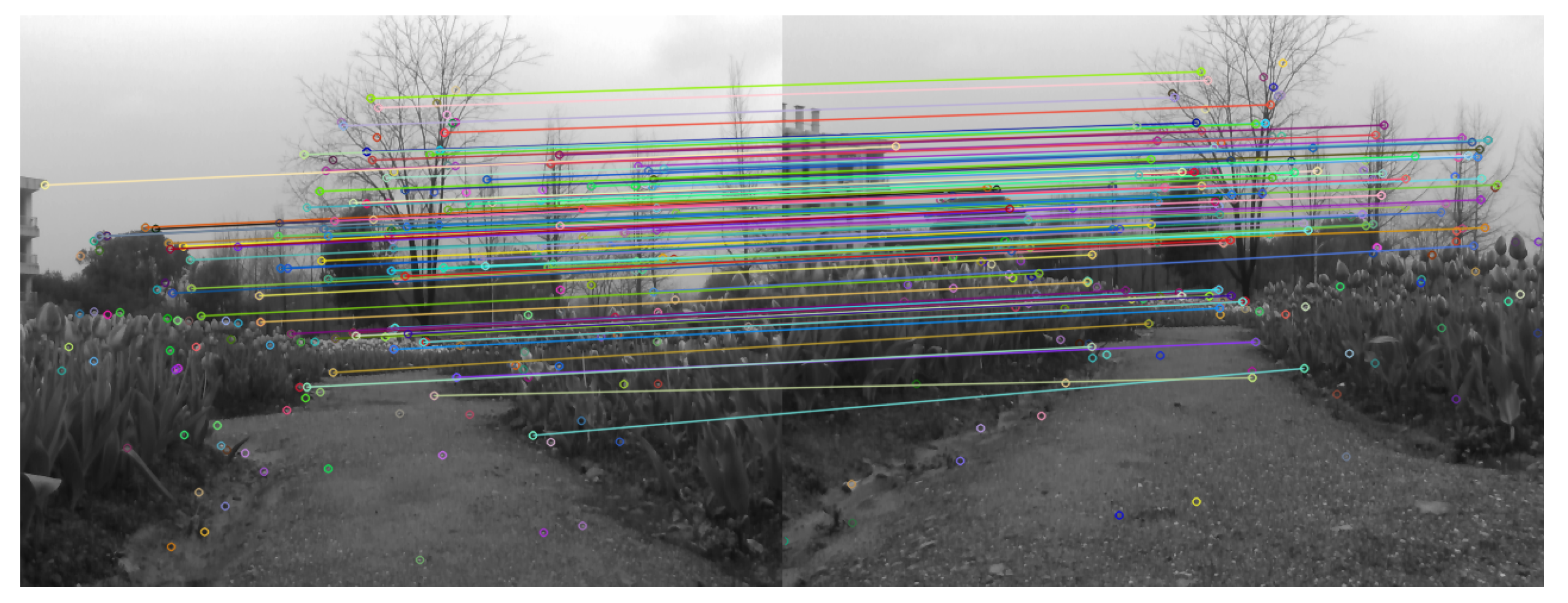
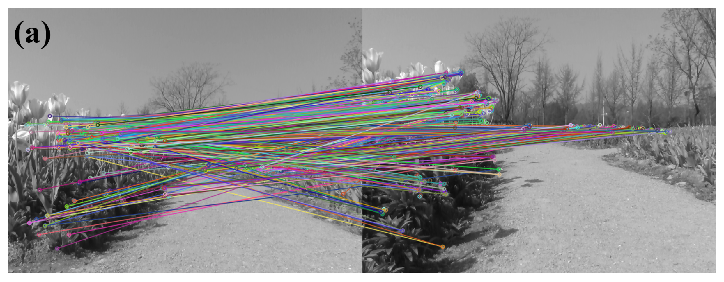
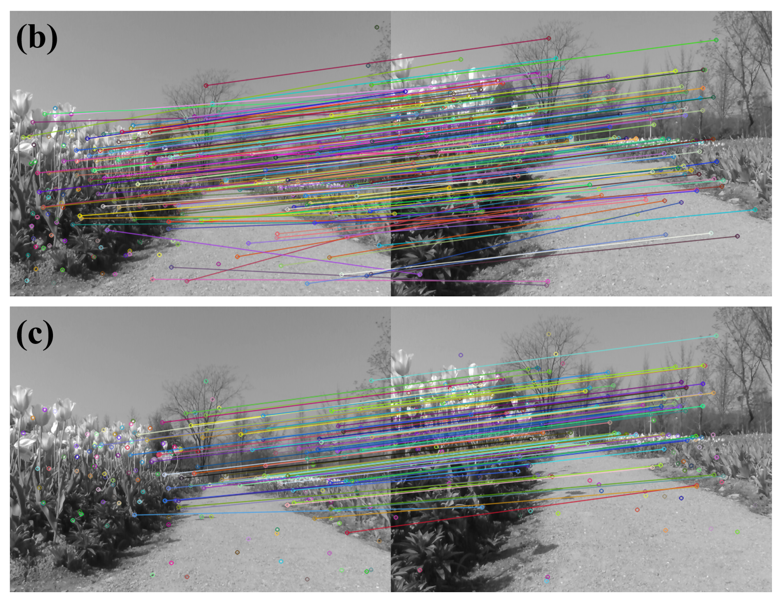
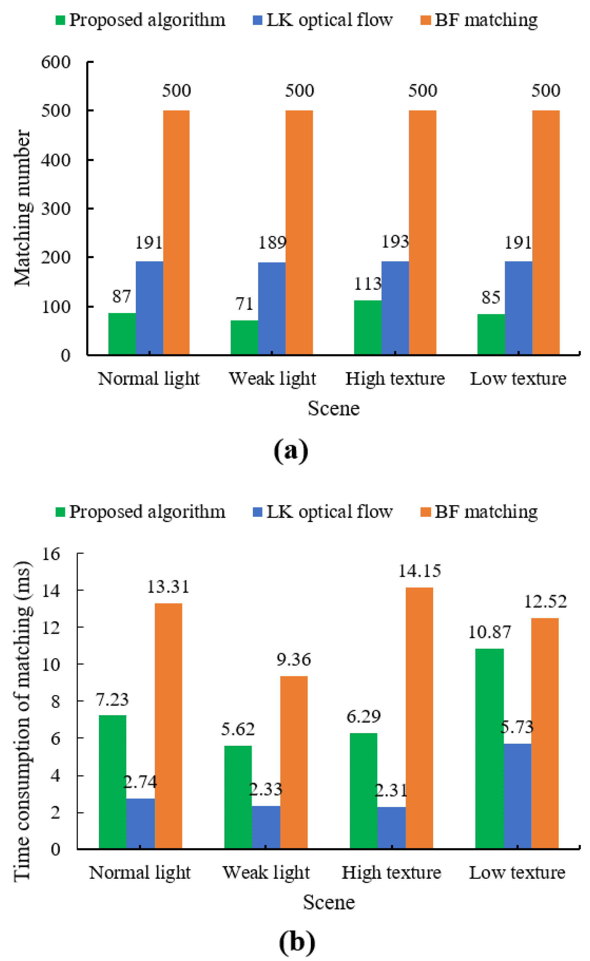
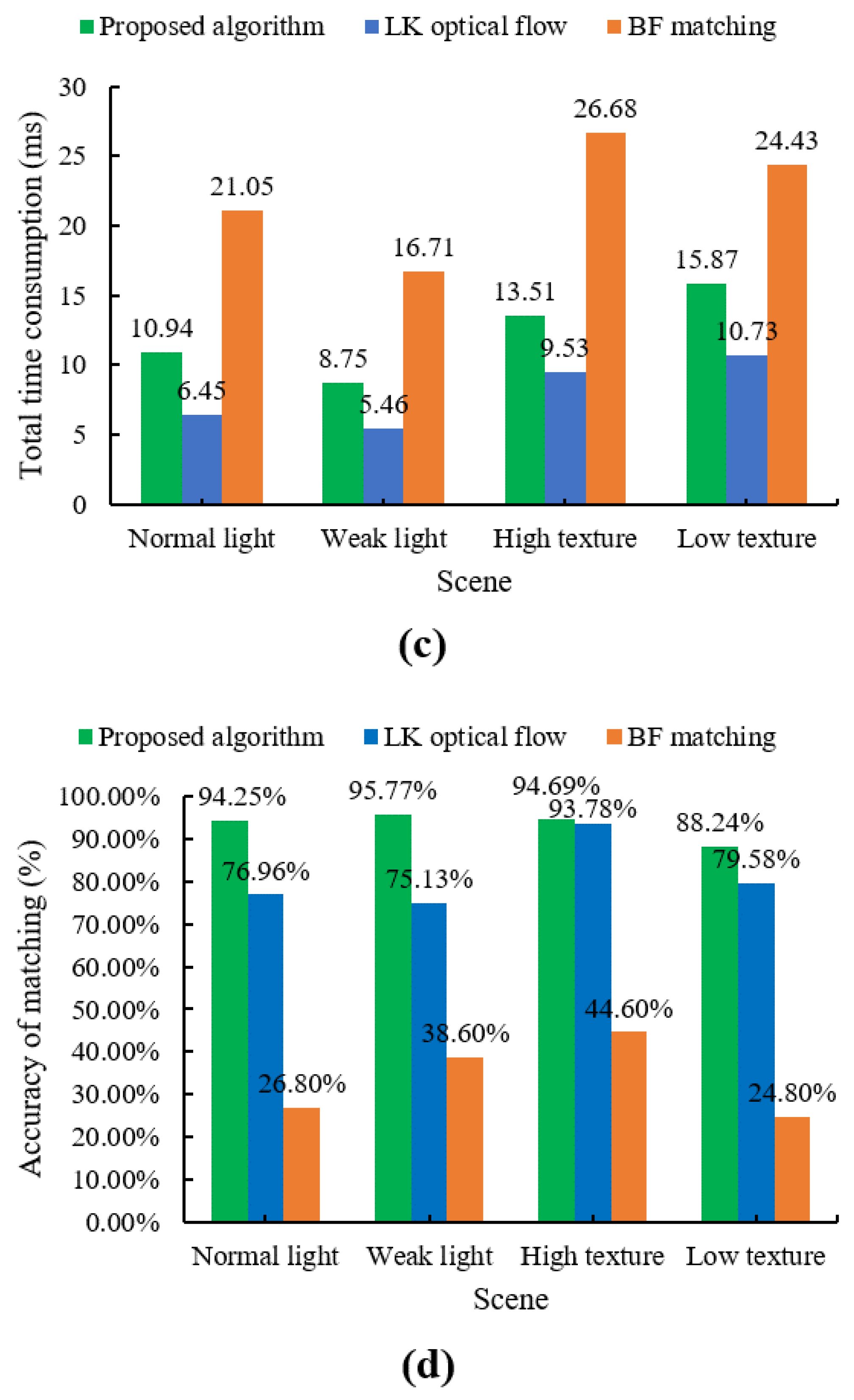
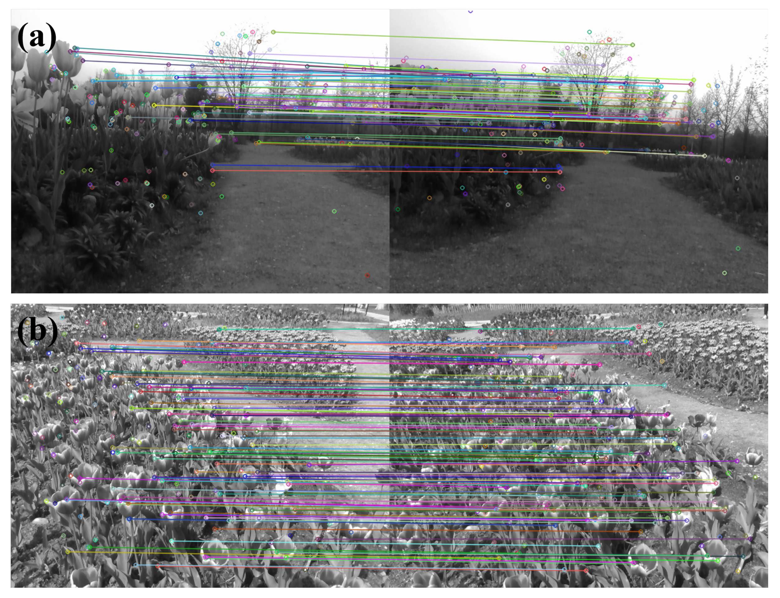
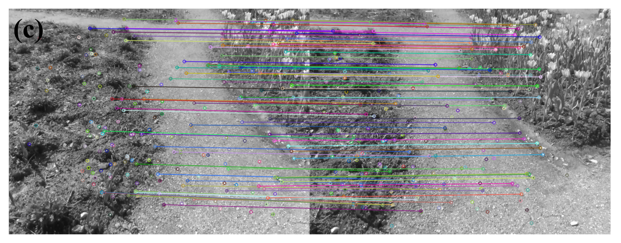
3.2. Accuracy and Analysis of Feature Matching
3.2.1. Results
3.2.2. Discussion
4. Conclusions
Author Contributions
Funding
Data Availability Statement
Acknowledgments
Conflicts of Interest
References
- Mur-Artal, R.; Montiel, J.; Tardos, J. ORBSLAM: A Versatile and Accurate Monocular SLAM System. IEEE Trans. Robot. 2015, 31, 1147–1163. [Google Scholar] [CrossRef]
- Chen, M.; Tang, Y.; Zou, X.; Huang, K.; Huang, Z.; Zhou, H.; Wang, C.; Lian, G. 3D global mapping of large-scale unstructured orchard integrating eye-in-hand stereo vision and SLAM. Comput. Electron. Agric. 2021, 187, 106237. [Google Scholar] [CrossRef]
- Li, P.; Garratt, M.; Lambert, A. A monocular odometer for a quadrotor using a homography model and inertial cues. In Proceedings of the IEEE International Conference on Robotics and Bio-mimetics, Zhuhai, China, 6–9 December 2015; pp. 570–575. [Google Scholar]
- He, Z.; Shen, C.; Wang, Q.; Zhao, X.; Jiang, H. Mismatching Removal for Feature-Point Matching Based on Triangular Topology Probability Sampling Consensus. Remote Sens. 2022, 14, 706. [Google Scholar] [CrossRef]
- Rublee, E.; Rabaud, V.; Konolige, K.; Bradski, G. ORB: An efficient alternative to SIFT or SURF. In Proceedings of the IEEE International Conference on Computer Vision, Colorado Springs, CO, USA, 20–25 June 2011; pp. 2564–2571. [Google Scholar]
- Qin, Y.; Xu, H.; Chen, H. Image feature points matching via improved ORB. In Proceedings of the IEEE International Conference on Progress in Informatics and Computing, Shanghai, China, 16–18 May 2014; pp. 204–208. [Google Scholar]
- Huang, C.; Zhou, W. A real-time image matching algorithm for integrated navigation system. Optik 2014, 125, 4434–4436. [Google Scholar] [CrossRef]
- Xu, Z.; Liu, Y.; Du, S.; Wu, P.; Li, J. DFOB: Detecting and describing features by octagon filter bank for fast image matching. Signal Process. Image Commun. 2016, 41, 61–71. [Google Scholar] [CrossRef]
- Cai, L.; Ye, Y.; Gao, X.; Li, Z.; Zhang, C. An improved visual SLAM based on affine transformation for ORB feature extraction. Optik 2021, 227, 165421. [Google Scholar] [CrossRef]
- Luo, H.; Liu, K.; Jiang, S.; Li, Q.; Wang, L.; Jiang, W. CAISOV: Collinear Affine Invariance and Scale-Orientation Voting for Reliable Feature Matching. Remote Sens. 2022, 14, 3175. [Google Scholar] [CrossRef]
- Zhang, Y.; Zhou, P.; Ren, Y.; Zou, Z. GPU-accelerated large-size VHR images registration via coarse-to-fine matching. Comput. Geosci. 2014, 66, 54–65. [Google Scholar] [CrossRef]
- Shi, J.; Wang, X. A local feature with multiple line descriptors and its speeded-up matching algorithm. Comput. Vis. Image Underst. 2017, 162, 57–70. [Google Scholar] [CrossRef]
- Chen, S.; Shi, Y.; Zhang, Y.; Zhao, J.; Zhang, C.; Pei, T. Local multi-feature hashing based fast matching for aerial images. Inf. Sci. 2018, 442–443, 173–185. [Google Scholar] [CrossRef]
- Pang, S.; Du, A.; Mehmet, A.; Chen, H. Weakly supervised learning for image keypoint matching using graph convolutional networks. Knowl.-Based Syst. 2020, 197, 105871. [Google Scholar] [CrossRef]
- Saleem, S.; Bais, A.; Sablatnig, R. Towards feature points based image matching between satellite imagery and aerial photographs of agriculture land. Comput. Electron. Agric. 2016, 126, 12–20. [Google Scholar] [CrossRef]
- Fischler, M.; Bolles, R. Random Sample Consensus: A Paradigm for Model Fitting with Applications to Image Analysis and Automated Cartography. Commun. ACM 1981, 24, 381–395. [Google Scholar] [CrossRef]
- Xu, H.; Huang, T.; Liu, J. Image restoration with the SOR-like method. In Proceedings of the Sixth International Conference of Matrices and Operators, Prague, Czech Republic, 6–10 June 2011; Volume 2, pp. 412–415. [Google Scholar]
- Chung, K.-L.; Tseng, Y.-C.; Chen, H.-Y. A Novel and Effective Cooperative RANSAC Image Matching Method Using Geometry Histogram-Based Constructed Reduced Correspondence Set. Remote Sens. 2022, 14, 3256. [Google Scholar] [CrossRef]
- Furkan, K.; Baris, A.; Hasan, S. VISOR: A fast image processing pipeline with scaling and translation invariance for test oracle automation of visual output system. J. Syst. Softw. 2018, 136, 266–277. [Google Scholar]
- Bruno, N.; Martani, M.; Corsini, C.; Oleari, C. The effect of the color red on consuming food does not depend on achromatic (Michelson) contrast and extends to rubbing cream on the skin. Appetite 2013, 71, 307–313. [Google Scholar] [CrossRef]
- Furgale, P.; Rehder, J.; Siegwart, R. Unified temporal and spatial calibration for multi-sensor systems. In Proceedings of the IEEE/RSJ International Conference on Intelligent Robots and Systems, Tokyo, Japan, 3–7 November 2013; pp. 1280–1286. [Google Scholar]
- Tafti, A.; Baghaie, A.; Kirkpatrick, A. A comparative study on the application of SIFT, SURF, BRIEF and ORB for 3D surface reconstruction of electron microscopy images. Comput. Methods Biomech. Biomed. Eng. Imaging Vis. 2018, 6, 17–30. [Google Scholar] [CrossRef]
- Bayh, H.; Tuytelaars, T.; Gool, L. SURF: Speeded up robust features. Comput. Vis. Image Underst. 2006, 110, 404–417. [Google Scholar]
- Guan, Q.; Wei, G.; Wang, Y.; Liu, Y. A dual-mode automatic switching feature points matching algorithm fusing IMU data. Measurement 2021, 185, 110043. [Google Scholar] [CrossRef]
- Himanshu, R.; Anamika, Y. Iris recognition using combined support vector machine and Hamming distance approach. Expert Syst. Appl. 2014, 41, 588–593. [Google Scholar]
- Lucas, B.; Kanade, T. An Iterative Image Registration Technique with an Application to Stereo Vision. In Proceedings of the 7th International Joint Conference on Artificial Intelligence (IJCAI), Vancouver, BC, Canada, 24–28 August 1981; pp. 674–679. [Google Scholar]
- Rosin, P. Measuring Corner Properties. Comput. Vis. Image Underst. 1999, 73, 291–307. [Google Scholar] [CrossRef] [Green Version]
- Calonder, M.; Lepetit, V.; Strecha, C. Brief: Binary robust independent elementary features. In Proceedings of the European Conference on Computer Vision, Heraklion, Greece, 5–11 September 2010; pp. 778–792. [Google Scholar]


| Feature Point Set | Aggregation Rate c (%) | Uniformity |
|---|---|---|
| Nonuniformed | 60.42 | 0.08 |
| Uniformed | 21.42 | 0.44 |
| Scene | Traditional ORB Algorithm | Proposed Algorithm | ||||||
|---|---|---|---|---|---|---|---|---|
| t/ms | c/% | t/ms | c/% | |||||
| Normal light | 500 | 7.74 | 0.15 | 74.80 | 251 | 3.72 | 0.40 | 23.36 |
| Weak light | 500 | 7.34 | 0.16 | 69.43 | 250 | 3.13 | 0.40 | 12.02 |
| High texture | 500 | 12.53 | 0.29 | 61.46 | 249 | 7.22 | 0.47 | 14.28 |
| low texture | 500 | 11.92 | 0.31 | 57.39 | 250 | 5.03 | 0.51 | 11.56 |
Publisher’s Note: MDPI stays neutral with regard to jurisdictional claims in published maps and institutional affiliations. |
© 2022 by the authors. Licensee MDPI, Basel, Switzerland. This article is an open access article distributed under the terms and conditions of the Creative Commons Attribution (CC BY) license (https://creativecommons.org/licenses/by/4.0/).
Share and Cite
Chen, Q.; Yao, L.; Xu, L.; Yang, Y.; Xu, T.; Yang, Y.; Liu, Y. Horticultural Image Feature Matching Algorithm Based on Improved ORB and LK Optical Flow. Remote Sens. 2022, 14, 4465. https://doi.org/10.3390/rs14184465
Chen Q, Yao L, Xu L, Yang Y, Xu T, Yang Y, Liu Y. Horticultural Image Feature Matching Algorithm Based on Improved ORB and LK Optical Flow. Remote Sensing. 2022; 14(18):4465. https://doi.org/10.3390/rs14184465
Chicago/Turabian StyleChen, Qinhan, Lijian Yao, Lijun Xu, Yankun Yang, Taotao Xu, Yuncong Yang, and Yu Liu. 2022. "Horticultural Image Feature Matching Algorithm Based on Improved ORB and LK Optical Flow" Remote Sensing 14, no. 18: 4465. https://doi.org/10.3390/rs14184465