Assessment and Prediction of Impact of Flight Configuration Factors on UAS-Based Photogrammetric Survey Accuracy

Abstract

Recent advances in computer vision and camera-equipped unmanned aerial systems (UAS) for 3D modeling enable UAS-based photogrammetry surveys with high spatial-temporal resolutions. To generate consistent and high-quality 3D models using UASs, understanding how influence factors (i.e., flight height, image overlap, etc.) affect the 3D modeling accuracy and their levels of significance are important. However, there is little to no quantitative analysis that studies how these influence factors interact with and affect the accuracy when changing the values of the influence factors. Moreover, there is little to no research that assesses more than three influence factors. Therefore, to fill this gap, this paper aims to evaluate and predict the accuracy generated by different flight combinations. This paper presents a study that (1) assessed the significance levels of five influence factors (flight height, average image quality, image overlap, ground control point (GCP) quantity, and camera focal lengths), (2) investigated how they interact and impact 3D modeling accuracy using the multiple regression (MR) method, and (3) used the developed MR models for predicting horizontal and vertical accuracies. To build the MR model, 160 datasets were created from 40 flight missions collected at a site with a facility and open terrain. For validating the prediction model, five testing datasets were collected and used at a larger site with a complex building and open terrain. The results show that the findings of this study can be applied to surveyors’ better design flight configurations that result in the highest accuracies, given different site conditions and constraints. The results also provide a reasonable prediction of accuracy given different flight configurations.

1. Introduction

Small unmanned aerial systems (UAS) in conjunction with photogrammetric techniques have been widely used as they offer affordable operable costs and efficient and safe aerial data acquisition [1]. The technological development in advanced software and hardware has led to automatic data collection using UAS with different sensors based on user requirements [2]. These sensors include RGB digital cameras, thermal infrared cameras [3,4], multispectral camera [5,6], and Light Detection and Ranging (LiDAR) [7,8]. Nex et al. [9] reviewed the most prominent developments on UAVs for remote sensing and mapping applications using onboard sensors mentioned above. The best practices to follow using the existing technologies and their limitations have been reported.

UAS-based photogrammetric surveying and mapping applications are broadly applied in various fields to provide an accurate 3D point cloud model with a high spatial resolution. Studies on UAS range from forest and biomass [10,11], construction industry [12,13], crop and agriculture [14,15], coastline and riverbank [16,17], archaeologic [18,19], facility and road [20,21], inspection [22,23], to emergency mapping [24].

The accuracy of UAS-based photogrammetric surveying largely depends on the accuracy of structure-from-motion (SfM) techniques that reconstruct 3D scenes and estimate camera poses (location and orientations) from 2D images [25]. Förstner and Wrobel [26] provides a statistical treatment and algorithms of the geometry of multiple view analysis useful for camera calibration, orientation, and geometric scene reconstruction.

Previous research has shown that the accuracy is influenced by numerous factors, such as flight heights [27], UAS-equipped camera sensors and settings [27,28,29,30], image overlaps [11,31], ground control points (GCP) quantities and distributions [30,32], georeferencing methods [14,33], and processing SfM software utilization [30,34]. To generate consistently high-quality 3D models from UAS-based photogrammetric surveying and mapping, understanding how these influence factors affect the model accuracy and their levels of significance is important. Moreover, since the site conditions change, understanding what accuracy can be achieved and designing optimal flight paths based on site constraints or limitations is an essential procedure to produce high-quality 3D models.

However, most previous research only focuses on the influence of no more than three important factors [12,35]. No research uses a quantitative method to analyze more than three influence factors, discuss which factors have a higher or lower impact on accuracy, and predict the level of accuracy based on the site conditions and flight configuration influence factors. Moreover, some surveyors do not know what accuracy to expect and largely make guesses based on their prior knowledge. Those without experience cannot even guess what accuracy to expect other than good accuracies that software providers use in marketing which often do not translate to reality [36].

Thus, to fill this research gap, the main objective of this paper is to (1) assess five major influence factors, (2) identify their levels of significance on horizontal and vertical accuracies, and (3) predict the horizontal and vertical accuracies of different combinations of influence factors using the multiple regression (MR) method. The influence factors include:

(1)

flight height,

(2)

flight overlap,

(3)

the quantity of GCPs,

(4)

the focal length of the camera lens, and

(5)

the average image quality of each image dataset.

To assess the influence factors and build the MR model, UAS-based surveying images using different sets of flight configurations were collected at a facility with an open field in Raleigh, NC. To validate the MR model, another set of images was collected at a test site that has a larger facility and open terrain in Butner, NC. The horizontal and vertical accuracies are evaluated through the positional comparison of checkpoints (CPs) by following the industry standards [37]. The main contributions of this paper are as follows:

(1)

Evaluation of five main influence factors of UAS-based photogrammetric surveying and their significance level using the MR method.

(2)

MR modeling for prediction of the UAS-based photogrammetric accuracy with different flight configurations.

With these contributions, this study can help surveyors better deal with different site constraints that affect the influence factors, design optimal flight configurations, and estimate the accuracy.

2. Background

This section presents the related studies on the impact of influence factors on UAS-based photogrammetric surveying accuracy.

Table 1. Overview of the Related Research.

Number of Influence Factors	Factors	Authors	Research Description	Highest MAE/RMSE Horizontal	Highest MAE/RMSE Vertical
Single Influence Factors	Flight Height	[27]	Evaluate the influence of flight height and area coverage orientations on the DSM and orthophoto accuracies for flood damage assessment.	N/A (consistently lower than 0.05 m, i.e., not more than 1–2 pixels)	N/A
		[30]	Provide a solution of data collection and processing of UAS application in complex forest environment	N/A	N/A
	GCP Quantity and Distribution	[10]	Assess the influence of numbers of GCPs on DSM accuracy.	N/A	0.057 m
		[19]	Propose an algorithm to calculate the sparse point cloud roughness using associated angular interval.	N/A	N/A
		[28]	Evaluate the impact of GCP quantities on UAS-based photogrammetry DSM and orthoimage accuracies.	0.053 m	0.049 m
		[35]	Assess the influence of different grades of tree covers and GCP quantities and distributions on UAS-based point cloud in forest areas.	0.031 m	0.058 m
		[2]	Evaluate the influence of additional GCPs on spatial accuracy when AAT is applied for georeferencing.	N/A	N/A
		[38]	Identify the GCP quantities and distributions to generate a high accuracy for a corridor-shaped site.	0.027 m	0.055 m
		[39]	Evaluate the effect of the location and quantity of GCPs on UAS-based DSMs in Glaciers.	N/A	N/A
		[40]	Evaluate the impact of GCP quantities and distributions on UAS-based photogrammetry DSM and orthoimage accuracies.	0.035 m	0.048 m
		[41]	Provide a solution about the optimal GCP quantity to generate high precision 3D models.	N/A	N/A
		[42]	Provide information of the optimal GCP deployment for dam structures and high-rise structures.	0.057 m	0.012 m
		[43]	Analyze the influence of the quantities and numbers of GCPs on 3D model accuracy.	N/A	N/A
		[44]	Analyze the influence of GCP quantities on UAS photogrammetric mapping accuracy using RTK-GNSS system.	N/A	0.003 m
		[45]	Analyze 3D model and DSM accuracies to determine the optimal GCP quantities in various terrain types.	0.044 m	0.036 m
	Camera Setting	[32]	Analyze the influence of photogrammetric process elements on the quality of UAS-based photogrammetric accuracy to identify artificial lighting at night	N/A	N/A
		[34]	Evaluate the influence of camera sensor types and configurations and SfM processing tools on UAS mapping accuracy.	N/A	N/A
		[46]	Analyze the influence of the ground control quality and quantity on DEM accuracy using a Monte Carlo Method.	N/A	N/A
		[47]	Generate a larger virtual image from five head cameras	2.13 pixels	N/A
		[48]	Investigate three issues of corridor aerial image block, including: focal length error, a gradually varied focal length, and rolling shutter effects.	0.007 m	0.008 m
	Image Acquisition	[29]	Evaluate the impact of image parameters on the close-range UAS-based photogrammetric inspection accuracy.	N/A	N/A
		[49]	Evaluate the impact of image formats and levels of JPEG compression in UAS-based photogrammetric accuracy.	N/A	N/A
		[50]	Evaluate the influence of low-height UAS photogrammetry systems on stable images, data processing and accuracy.	N/A	0.059 m
	Georeferencing Methods	[1]	Introduces a custom-built multi-sensor system for direct georeferencing.	0.012 m	0.020 m
		[14]	Evaluate the impact of GNSS receivers of techniques features and working modes on positioning accuracy.	N/A	N/A
		[15]	Evaluate the geometric accuracy of using four different georeferencing techniques	0.023 m	0.03 m
		[33]	Evaluate the quality of photogrammetric models and DTMs using PPK and RTK modes in coastline areas.	N/A	0.016 m
		[51]	Analyze the impact of UAS blocks and georeferencing methods on accuracy and repeatability.	0.016 m	0.014 m
		[52]	Evaluate the influence of image block orientation methods on the accuracy of estimated forest attributes, especially the plot mean tree height.	N/A	N/A
		[53]	Analyze the influence of different UAS platforms on positional and within-model accuracies without GCPs.	N/A	N/A
		[54]	Provide operational guidelines and best practices of direct georeferencing methods on positional accuracy.	N/A	0.019 m
		[55]	Assess the influence of GNSS with PPK on the UAS-based accuracy in building surveying applications.	N/A	0.01 m
		[56]	Assess the influence of RTK/PPK on geospatial accuracies of photogrammetric products in forest areas.	0.003 m	0.006 m
	Flight Height and Image Acquisition	[11]	Provide scientific evidence of the impact of flight height, image overlap, and image resolution on forest area reconstruction.	N/A	N/A
Multiple Influence Factors	GCP Quantity and Distribution and Georeferencing Methods	[12]	Evaluate the impact of cross flight patterns, GCP distributions, and RTK-GNSS on camera self-calibration and bundle block adjustment quality.	N/A	N/A
	Camera Setting and Image Acquisition	[31]	Evaluate the impact of image resolution, camera type, and side overlap on predicted biomass model accuracy.	N/A	N/A
	Flight Height and GCP Quantity and Distribution and Image Acquisition	[57]	Evaluate the impact of flight heights, terrain types, and GCP quantities on DSM and orthoimage accuracy in UAS-based photogrammetry	0.000169 m	0.047 m
		[58]	Evaluate the impact of flight height, image overlap, GCPs quantities and distribution, and time of survey on snow depth measurement.	N/A	N/A
		[59]	Analyze the impact of flight heights and quantities and distribution of GCPs on survey error.	N/A	N/A
	GCP Quantity and Distribution and Camera Setting	[60]	Evaluate the influence of camera calibration methods as well as quantities and distributions of GCPs on UAS photogrammetry accuracy.	1.3 mm	5.1 mm
	Flight Height and GCP Quantity and Distribution and Camera Setting	[61]	Assess the impact of flight height, image overlap, GCP quantities, and construction site conditions on measurement accuracy.	N/A	0.085 m

summarizes the area of the work and influence factors for accuracy checking. 41 articles from major journals in the related field are summarized. Additionally, the highest accuracy achieved for each article is also summarized in Table 1. The highest accuracy values were reported using mean absolute error (MAE) or root mean square error (RMSE). N/A presents there is no highest value reported in the article. The following subsections are broken down by these influence factors that impact UAS-based photogrammetric surveying accuracy.

2.1. Flight Heights

Studies indicate that flight heights can impact the accuracy of the UAS-based photogrammetry. Research conducted by [27] assessed the accuracy of UAS image data using different flight heights (126–235 m) in a semi-arid and medium-relief area with flood damage. The assessment was with respect to the MAE of the vertical and horizontal accuracies of the generated digital surface model (DSM). The results indicated that the MAE in the vertical direction was increased with the increase in flight heights, while the MAE in the horizontal direction was maintained stable (consistently lower than 0.05 m, i.e., not more than 1–2 pixels).

2.2. Image Overlap

Previous research showed that varying image overlaps could influence the accuracy of UAS-based photogrammetry. The influence of image overlap on the accuracy of UAV-photogrammetry-based snow depth distribution maps was studied by [48]. This research applied three different image overlaps were applied in this research, including 90% front overlap by 81% side overlap, 80% front overlap by 72% side overlap, and 70% front overlap by 63% side overlap. The results demonstrated that accuracy would be improved when increasing the image overlap.

2.3. GCP Quantities and Distribution

The reports show that less than ¼ ground sample distance (GSD) accuracy can be achieved when the pre-calibrated camera-equipped UAS is flying over 100 m above ground level (AGL), even if using the minimum GCP quantities. Due to the low stability of the optical system, a large number of GCPs were required for the UAS using the direct orientation method. A pre-calibrated camera is a type of camera calibration method which is performed prior to the bundle adjustment in the SfM workflow. When pre-calibration is performed, all camera settings should be fixed. The camera can be calibrated using a chessboard to observe it from different angles [62].

Previous research showed consistent results regarding the influence of the number and location of GCPs used to assess accuracy. Increasing the number of GCPs would improve accuracy in both horizontal and vertical directions. Additionally, well-distributed GCPs could generate more accurate results than using randomly distributed GCPs. Research conducted by [10,19] determined that using GCPs would yield better accuracy than without using GCPs. The research conducted by [19] used 39 GCPs in a 0.22 ha size. The study conducted by [10] compared the results of using zero, five, and ten GCPs in an 80 ha study area. The results showed that the RMSE of using zero, five, and ten GCPs were 2.255, 0.072, and 0.057 m. The study conducted by [54] used 3465 different combinations of GCPs in bundle adjustment to answer the question about the best displacement of GCPs to achieve the desired accuracy. 102 targets were evenly distributed throughout a highland and mining area with 1225 ha. Among all the targets, the numbers of GCPs used in this research were from three to 101. Results demonstrated that the accuracy achieved by using evenly distributed GCPs could be twice as good as that of poorly distributed GCPs. Additionally, utilizing the medium to high numbers of GCPs (i.e., 3 GCPs per 100 photos), could obtain the desired accuracy. The research conducted by [38] investigated the impact of various numbers of GCPs on DSM and orthoimages. This research was conducted on a sloping site with a size of 18 ha. The numbers 4, 5, 6, 7, 8, 9, 10, 15, and 20 GCPs were used. The optimal accuracy was derived using 15 GCPs. Optimal results for RMSE_X, RMSE_Y and RMSE_XY mean ± standard deviation values were reached for 15 GCPs: 3.3 ± 0.346, 3.2 ± 0.441, 4.6 ± 0.340 and 4.5 ± 0.169 cm, respectively. Similar conclusions were derived for vertical accuracy: lower RMSE_Z mean ± standard deviation values were reached for 15 and 20 GCPs: 5.8 ± 1.21 cm and 4.7 ± 0.860 cm, respectively. The generated accuracies from 15 GCPs had no noticeable difference.

2.4. Georeferencing Methods

In addition to the aforementioned influence factors, some research investigated how georeferencing methods affect UAS-based photogrammetric surveying accuracy. The study studied by [14] compared the positional accuracy using various global navigation satellite systems (GNSS) receivers for mapping in agriculture. Their study demonstrated that the GNSS receivers with an external antenna could yield better positioning accuracy. The accuracy and repeatability of UAV block orientation by GNSS-supported orientation were researched by [40]. The impact on the checkpoint errors of the precision given to the projection centers had been studied. The results showed that with at least one GCP, the geocoding accuracy of GNSS-supported orientation was almost as good as that of a traditional GCP orientation in the horizontal direction and only slightly worse in the vertical direction. The highest accuracy in horizontal and vertical directions were 0.016 and 0.014 m. The research studied by [46] compares three image orientation methods on the accuracy of forest inventory attributes. The three image orientation methods were the Indirect Sensor Orientation (ISO) with five irregularly distributed GCPs, GNSS -supported Sensor Orientation (GNSS-SO) using non-Post Processed Kinematic (PPK) single-frequency carrier-phase GNSS data (GNSS-SO₁), and GNSS-supported Sensor Orientation (GNSS-SO) using PPK dual-frequency carrier-phase GNSS data (GNSS-SO₂). The results GNSS-SO₂ produced the highest accuracy while the ISO method generated the lowest accuracy. A custom-built multi-sensor system for direct georeferencing was proposed by [1] enabled georeferencing to be performed without access to the mapping area. This system combined GNSS receiver with Real-Time Kinematic (RTK) and inertial navigation system (INS) to achieve high accuracy. This system was tested using 30 test points and reported using RMSE. The results showed that this system with micro or light UASs could ensure centimeter-level object accuracy. The highest accuracies in horizontal and vertical directions were 0.012 and 0.020 m using six well-distributed GCPs and the indirect georeferencing method.

2.5. Multiple Factors

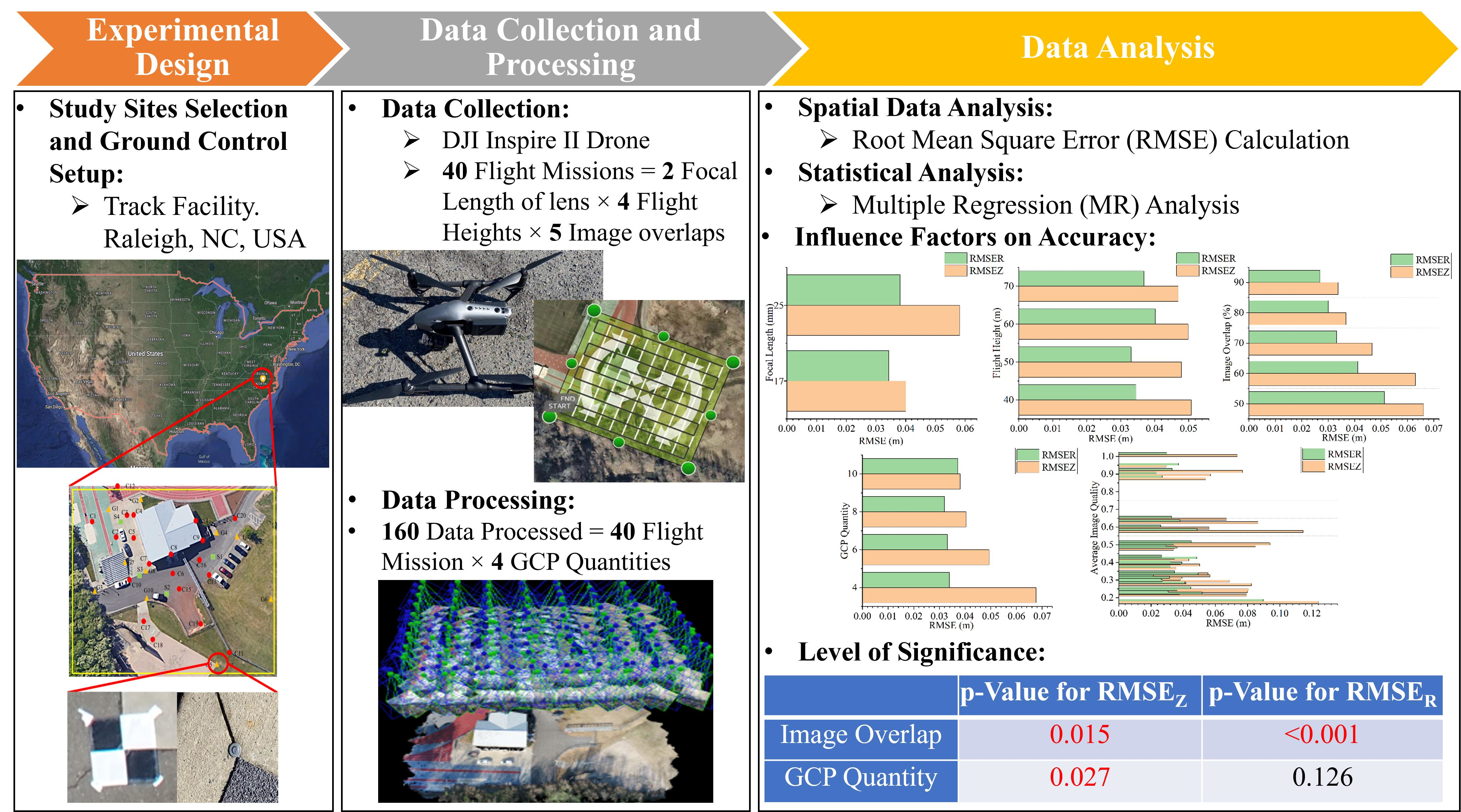
Out of those 40 papers, eight analyzed the influence of multiple influence factors on UAS-based photogrammetric surveying accuracy. None of them studied relative influences among these factors. The impact of image resolution, camera type, and side overlap on the prediction accuracy of biomass terrain types using multiple linear regression models was evaluated by [31]. Two different image resolutions (10 and 15 cm ground sampling distance), two camera types (NIR and RGB), and two different side overlap levels (70 and 80%) were assessed in their research. The results indicated that using the NIR camera could generate higher prediction errors than the RGB camera. A fine resolution improved the prediction accuracy regardless of the camera types. Additionally, increasing the side overlap decreased the prediction accuracy. However, there is no significant difference in image resolution, camera type, and side overlap on the accuracy of the 95% confidence level.

The research was conducted by [57] assessed the accuracy of the positional errors under various flight parameters, consisting of four flight heights (18 m (30 ft), 27 m (60 ft), 37 m (90 ft), and 46 m (150 ft)), two overlaps (70% and 90%), six different quantities of GCPs (zero, one, four, eight, twelve, and sixteen), and varying construction materials (sand, clay, fine grade gravel, and coarse grade gravel). In their research, multiple comprehensive comparisons and multiple regression analyses were used to observe the significance of the influence factors. The results showed that increasing the numbers of GCPs and image overlap would improve the accuracy. When the image overlap was low, increasing flight height could reduce the errors. Moreover, this research indicated that the quantity of GCPs had the most significant influence on the accuracy of the 95% confidential level. The highest accuracy of DSM (0.085 m) was achieved using low flight height (18 or 27 m) with high image overlap (90–60%) using more than twelve GCPs.

The study conducted by [11] researched the influence of image overlap, flight height, and camera sensor resolution on accuracy using a multivariate generalized additive model to set flight parameters for UAS-based surveying in forest areas optimally. Five different flight heights ranging from 25 m to 100 m (25 m, 40 m, 50 m, 75 m, and 100 m), four different image-side overlaps (67%, 55%, 45%, and 35%), and five various image resolutions (3840 × 2160 (100%), 2880 × 1620 (75%), 1920 × 1080 (50%), 960 × 540 (25%), and 768 × 432 (20%)) were utilized in this research. The results showed that low flight heights and high image overlaps could generate high accuracy with great reconstruction details and precision.

A case study carried by [28] evaluated the influence of flight heights, terrain morphologies, and the number of GCPs on DSM and orthoimage accuracies. Five terrain morphologies, four flight heights (50 m, 80 m, 100 m, and 120 m), and three different numbers of GCPs (3, 5, 10) were considered in this research. The results of this research presented that the quantity of the GCP was the most important factor affecting both horizontal and vertical accuracies. Increasing the number of GCPs would improve both horizontal and vertical accuracies. However, the result of terrain morphology was the opposite. The terrain morphology did not influence either horizontal or vertical accuracies. Although flight height did not influence horizontal accuracy, it impacted vertical accuracy. Vertical accuracy decreased as flight altitude increased. Moreover, this research found the most accurate combination of flight altitude and number of GCPs was 50 m and 10 GCPs, respectively, which yielded RMSE_X, RMSE_Y, RMSE_XY, and RMSE_Z values equal to 0.038, 0.035, 0.053, and 0.049 m, respectively

The research conducted by [61] used three different flight heights (67 m, 91 m, and 116 m), six different quantities of GCPs (5, 7, 9, 11, 13, and 15), and nine different types of GCP distributions on DSM accuracy in a complex and developed coastline. The results indicated that both horizontal and vertical accuracies increased as flight heights or the number of GCPs increased. For the GCP distributions, the accuracy was highest when GCPs were located in the corner, both high and low elevations of the study site.

Moreover, the research performed by [44] was about the accuracy assessment of the quantities of GCPs and the camera calibration methods. Similar to other research, their results also showed that accuracy would be improved with increasing GCP quantities. Moreover, the results presented that when capturing nadir images, there was no noticeable difference between using pre-calibration and self-calibration. However, when processing oblique images, adopting self-calibration could yield higher horizontal accuracy than pre-calibration.

A method proposed by [63] predicted the mapping quality from the information that was available prior to the flight, such as the flight plan, expected flight time, approximate digital terrain model, prevailing surface texture, and embedded sensor characteristics. They compared the quality prediction with the actual mapping accuracy in various geometrical configurations and the quality of the airborne GNSS positioning in the mountain environment. The results showed a satisfactory agreement.

According to the above literature, most previous research focused on flight height, GCP quantities, and image overlap but not image quality and focal length of the camera lenses. Additionally, most previous research simply assessed the accuracy through results comparisons using different influence factors values.

3. Methodology

Figure 1 shows the workflow of the methodology. An experiment was designed by selecting a site for a case study and planning data collection strategies. A case study was conducted at a facility site with open terrain. The indirect georeferencing method with GCPs and CPs was used. UAS flight missions were designed before data collection. A terrestrial laser scanning (TLS) was used for generating the coordinates of CPs for spatial accuracy evaluation. Pix4DMapper (one of the most widely used 3D reconstruction software by the company Pix4D founded in Swiss in 2011) was used to process the image data that was collected by a camera-equipped UAS. Next, the RMSE at the CPs was used to calculate spatial accuracy in horizontal and vertical directions. An MR model was developed to statistically analyze the factors’ significance and influence and predict the UAS-based photogrammetry accuracy based on the information of influence factors. Finally, the results of the MR model were validated using another test site. The following subsections here steps in detail.

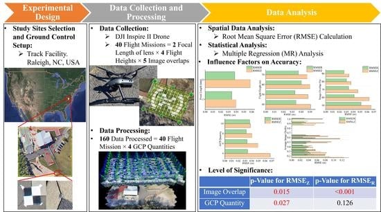
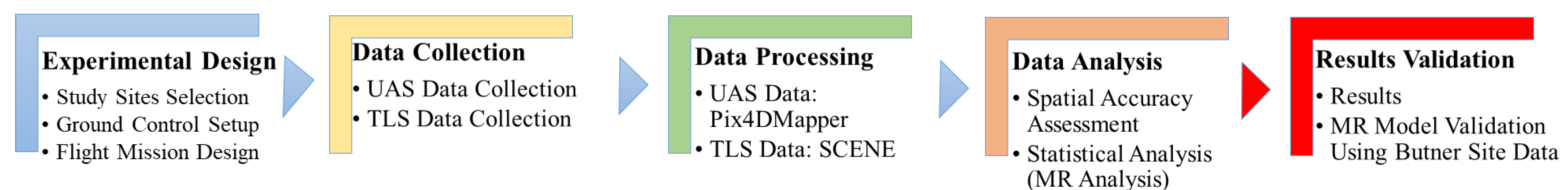
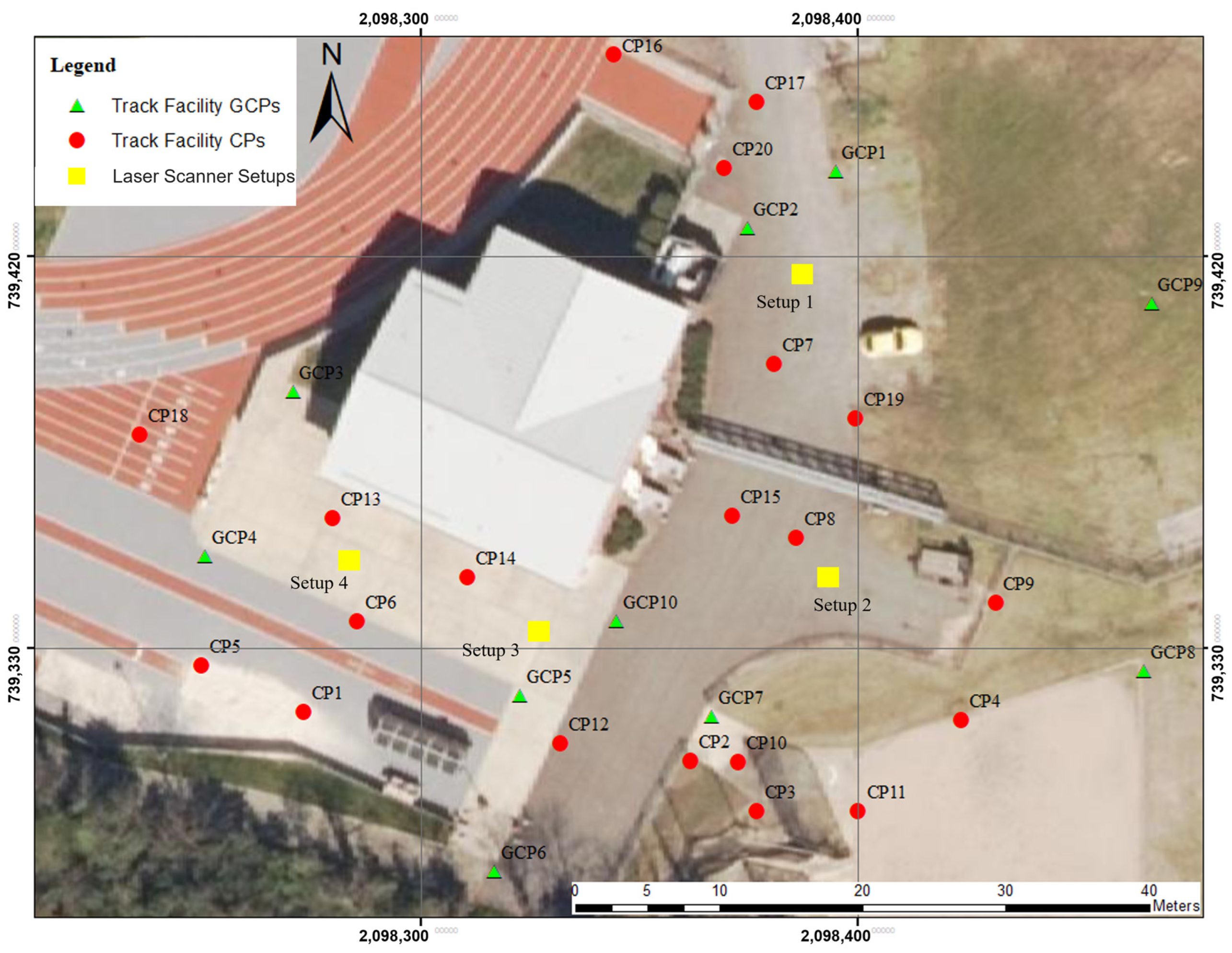
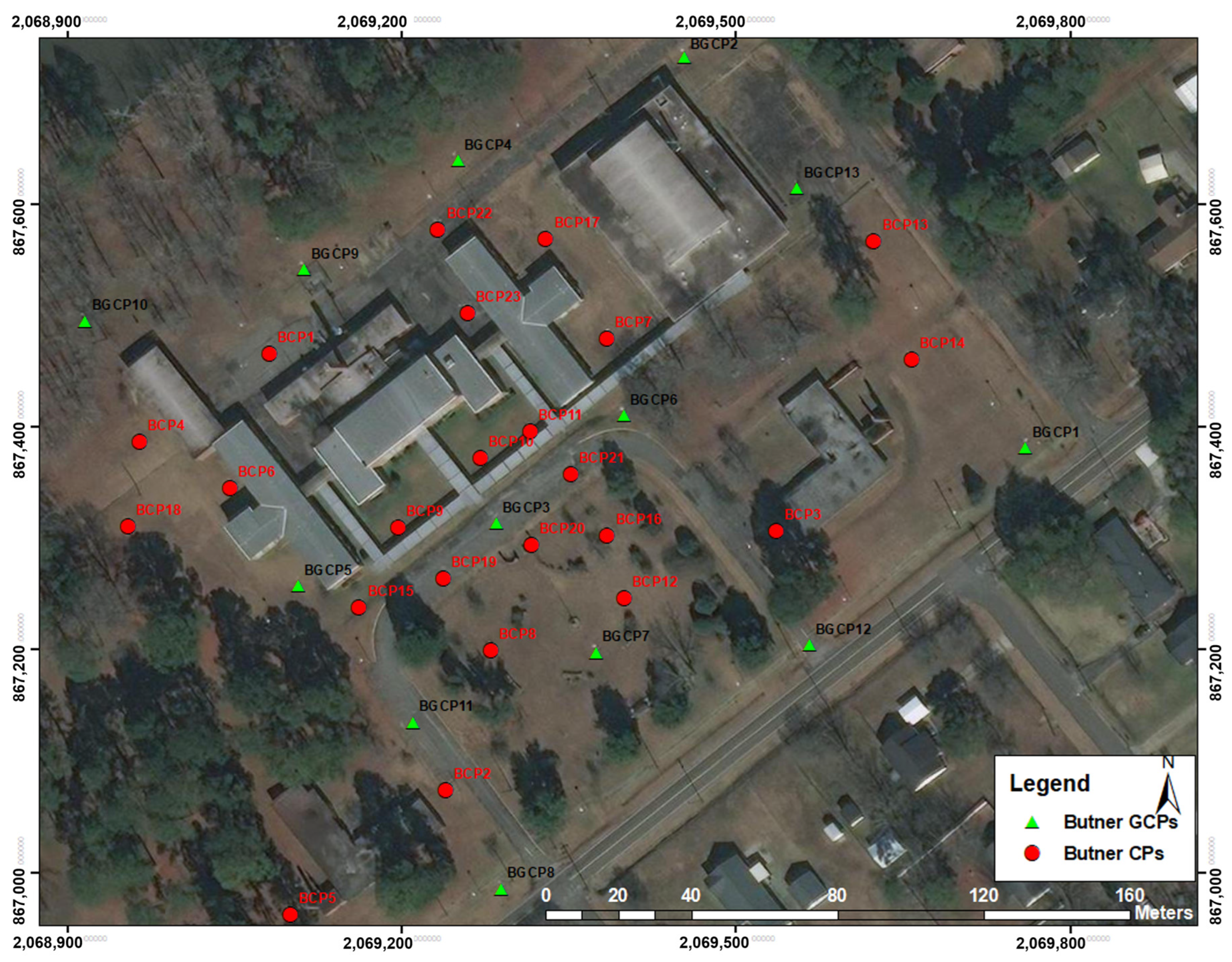
3.1. Experimental Design

A track facility site on the North Carolina State University (NCSU) campus in Raleigh, North Carolina, was selected to assess the influence factors. The size of this site is 0.49 ha. Figure 2 shows the site condition. This site contains a building facility, open space, and vegetation. The study area is shown in the yellow rectangle.

According to [37], no fewer than 20 CPs should be used in all accuracy observations since it might cause inaccurate results. Thus, 20 CPs are adopted to assess the RMSE errors in horizontal and vertical directions. Figure 3 shows the layout of the GCPs and CPs on the study site. As shown in the figure, 10 GCPs and 20 CPs were distributed around the site using PK nails and checkerboards (see Figure 4). The size of the checkboard marker is 24″ × 24″. There are four corner anchor points included to affix to the ground.

The coordinate system for the horizontal direction was the North American Datum (1983) (NAD83) (National Adjustment of 2011), State Plane Coordinate System, North Carolina Zone. The North American Vertical Datum (NAVD) of 1988 was used for the vertical coordinate system.

To assess influence factors, multiple flight configurations with different values of influence factors were designed. For instance, the flight heights were determined to be between 40 m and 70 m, and the GCP quantities between 4 and 10, which is reasonable as the size of the track facility site at NCSU was only 0.49 ha. Moreover, image overlap was decided to be from 50% to 90%. A short (25 mm) and a long (17 mm) focal length of camera lenses were needed to investigate the influence and significance. Thus, four different flight heights, five different image overlaps, four various quantities of GCPs, two different focal lengths of camera lenses were chosen. The average image quality was calculated based on all the images in each dataset. The quality of each image was calculated based on the comparison of the contrast gradients in the most peculiar areas between the original image and the Gaussian blur filter applied image through the Agisoft Photoscan Estimate Image Quality tool.

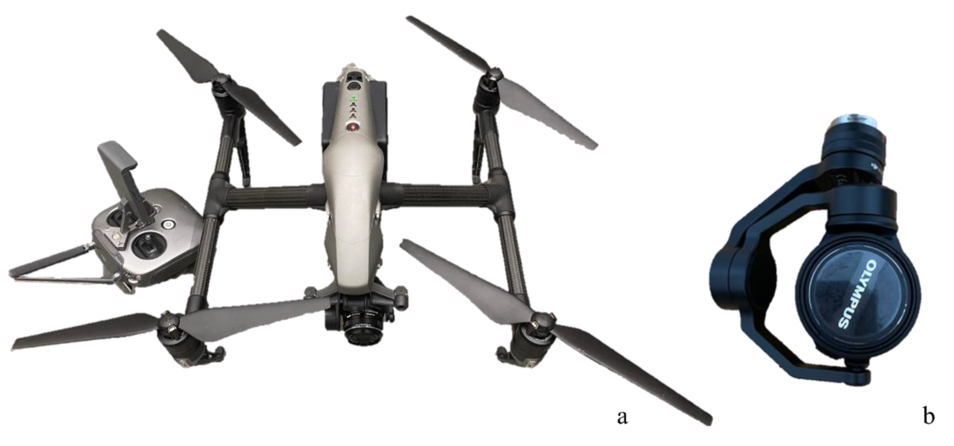
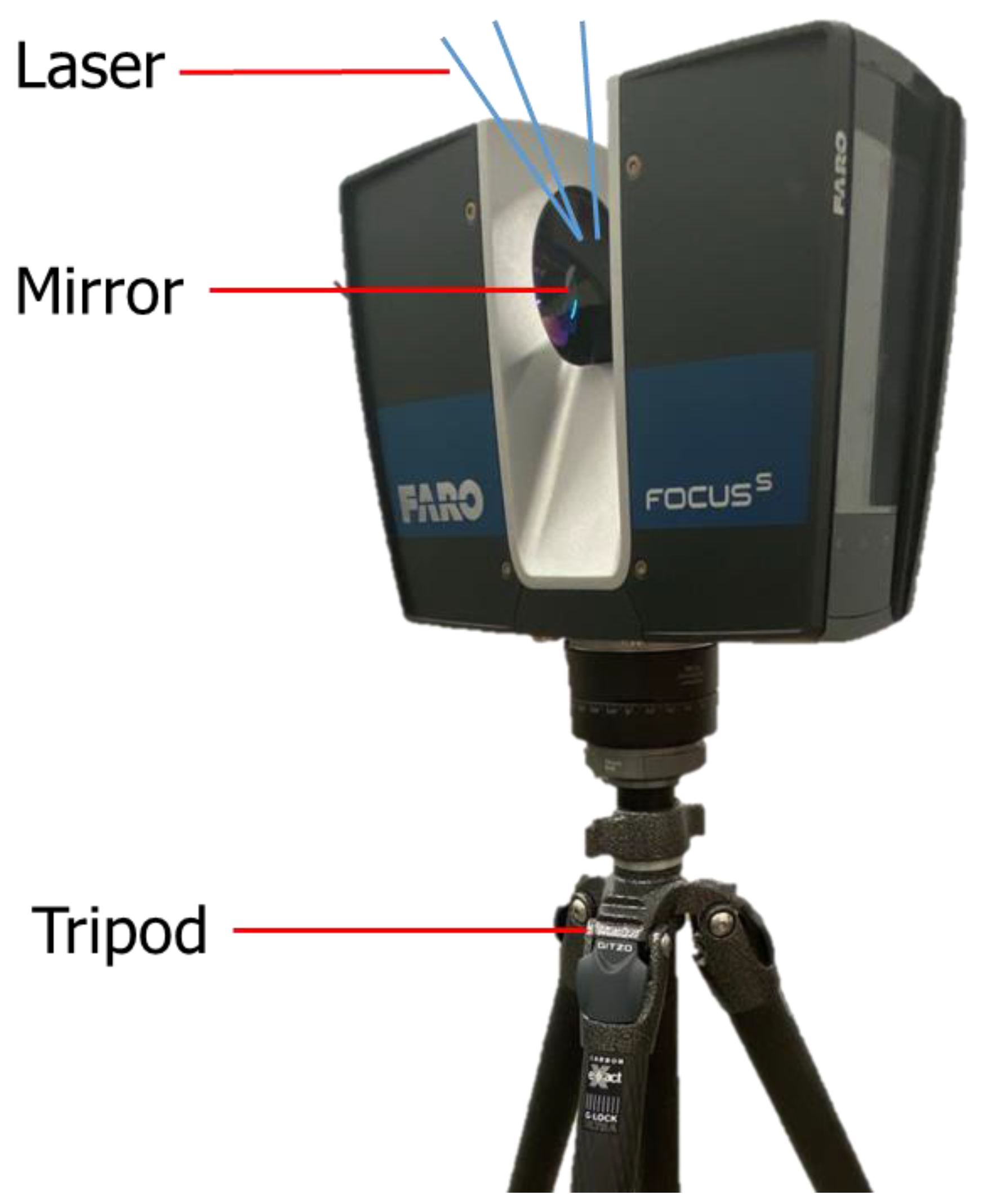
3.2. Data Collection

The UAS data and laser scan data collection at the NCSU track facility site took place from 19 January 2021, to 24 January 2021, from 10 a.m. to 3 p.m. to obtain optimal light conditions. The temperature ranged from 5 °C (41 °F) to 17 °C (57 °F). The wind speed was between 0.56 m/s (1.2 mph) and 3.61 m/s (8.0 mph) with a westerly wind direction. The information was obtained from Finding the Past weather through the National Weather Service website. The UAS image data was collected using a DJI (Da-Jiang Innovations, a Chinese technology company) Inspire II drone with a DJI Zenmuse X5S camera and an Olympus M.Zuiko (a Japanese manufacturer of optics and reprography products) 25 mm and 17 mm focal length lenses (Figure 5).

The flight missions were conducted by Pix4DCapture (a mobile app used to collect data) using autopilot mode. A double grid path was used as the flight path. The angle of the camera was 80° (oblique images). The autopilot mode allows an unmanned aerial vehicle, such as a drone, to perform entire missions autonomously without the need for manual remote control [64]. The UAS speed was Normal plus mode to save flight time. The white balance of the image was sunny. The following are the detailed flight configurations used to collect the data at the track facility site.

• Flight Heights: 40 m (131 ft), 50 m (164 ft), 60 m (197 ft), and 70 m (229 ft)
• Image Overlap: 50%, 60%, 70%, 80%, and 90%
• Focal Length: 17 mm and 25 mm

40 flight missions were conducted using different flight heights, image overlaps, and focal lengths of lenses. A total of 4425 images were collected for all flight missions. The number of collect images for every flight mission was 20 to 539. The average image quality of every image data set was between 0.18 and 1.01.

Table 2. Detailed Flight Mission Information.

Flight No.	Focal Length (mm)	Flight Height (m)	Overlap (%)	Average Image Quality	No. of Image
1	25	40	90	0.88	539
2	25	40	80	0.23	161
3	25	40	70	0.30	94
4	25	40	60	0.22	57
5	25	40	50	0.96	48
6	25	50	90	0.29	473
7	25	50	80	0.90	156
8	25	50	70	0.24	64
9	25	50	60	0.63	48
10	25	50	50	0.25	39
11	25	60	90	0.60	391
12	25	60	80	0.34	86
13	25	60	70	0.95	47
14	25	60	60	0.28	30
15	25	60	50	0.18	22
16	25	70	90	0.32	171
17	25	70	80	0.40	98
18	25	70	70	0.31	39
19	25	70	60	0.33	30
20	25	70	50	0.58	20
21	17	40	90	0.49	345
22	17	40	80	1.01	148
23	17	40	70	0.48	55
24	17	40	60	1.01	46
25	17	40	50	0.63	35
26	17	50	90	0.92	321
27	17	50	80	0.37	77
28	17	50	70	0.37	48
29	17	50	60	0.63	31
30	17	50	50	0.63	21
31	17	60	90	0.43	226
32	17	60	80	0.63	85
33	17	60	70	0.65	48
34	17	60	60	0.92	28
35	17	60	50	0.51	23
36	17	70	90	0.49	120
37	17	70	80	0.40	75
38	17	70	70	0.50	30
39	17	70	60	0.39	30
40	17	70	50	0.42	20

lists those 40 flight missions with detailed information.

FARO Focus S70 3D scanner (shown in Figure 6) was used to collect laser scans to produce the coordinates of CPs since the accuracy of laser scan registration was 2 mm, which was much less than the UAS photogrammetric surveying accuracy [65]. The field of views (FOV) in vertical and horizontal directions were 300° and 360°. FARO Focus S75 3D scanner was fit to a 1/5 resolution and 4× quality for scanning. Four setups (yellow squares S1–S4 in Figure 3) were adopted to cover the study area.

3.3. Data Processing

When processing the images for 3D reconstruction, 4, 6, 8, and 10 GCPs were used, leading to 160 combinations of datasets (40 flight configurations × 4 sets of GCPs). The data were processed based on the flight missions with different GCP quantities. UAS photogrammetric data were processed by Pix4DMapper version 4.4.6. Optimal settings were used in Pix4DMapper to achieve a high quality of accuracy.

Laser scans were processed in FARO SCENE (software to process and register all the laser scans) [66]. The laser scans were manually registered and georeferenced using the same coordinate system (North American Datum (1983) (NAD83) (National Adjustment of 2011), State Plane Coordinate System, North Carolina Zone).

The first step was to import the surveyed points into the workspace level in FARO SCENE as a reference. The surveyed points were the same set of ground control points used in UAS data processing. Those coordinates of surveyed points were collected using a GNSS receiver from the North Carolina Department of Transportation (NCDOT). Then, a three-point alignment method was used to match the coordinate system of the laser scans with the reference data (the imported surveyed points). A surveyed point was chosen as the new origin, and the X, Y, and Z values were entered for this point. After that, the coordinates of a second surveyed point were selected and entered to define the direction of the first axis. Next, the coordinates of another surveyed point were selected and entered to define the direction of the second axis. Finally, after applying all the changes, the coordinate system of the registered scans was automatically changed.

The registration error of the laser scans was 5.06 mm. The following

Table 3. Pix4DMapper Setting Parameters.

Processing Step	Parameters	Value
Alignment	Key points Image Scale	Full
	Image Scale for Alignment	Original Size
	Matching Image Pairs	Aerial Grid or Corridor
Calibration	Targeted Number of Key points	Automatic
	Calibration Method	Standard
Camera Optimization	Internal Parameters Optimization	All
	External Parameters Optimization	All
Dense Point Cloud Generation	Image Scale for Point Cloud Densification	Original Size with Multiscale
	Point Density	High
	Minimum Number of Match	3

and

Table 4. SCENE Setting Parameters.

Processing Step	Parameters	Value
Processing Setting	Colorization	Colorize Scans
	Find Targets	Find Checkerboards
Registration	Automatic Registration	Target Based
	Optimization and Verify	Cloud to Cloud

show the detailed settings of Pix4DMapper and SCENE.

3.4. Data Analysis

Data analysis includes two steps: spatial data analysis to assess the accuracy results of each dataset produced from Pix4DMapper, and statistical analysis to evaluate the level of significance and impact of influence factors and build the MR models to predict the accuracy.

3.4.1. Spatial Data Analysis

The [37] provides spatial accuracy metrics for reporting horizontal and vertical accuracy. The spatial accuracy was evaluated in easting (X), northing (Y), horizontal (R), and height (Z). Thus, the RMSE at CPs generated from Pix4DMapper showed the easting RMSE (RMSE_X), northing RMSE (RMSE_Y), horizontal RMSE (RMSE_R), and vertical RMSE (RMSE_Z). These values were computed as follows:

$${\mathrm{RMSE}}_{\mathrm{X}}=\sqrt{\frac{1}{n}{\displaystyle \sum }_{i=1}^n{\left({\mathrm{X}}_{i\left(ortho\right)}-{\mathrm{X}}_{i\left(survey\right)}\right)}^2}$$

(1)

$${\mathrm{RMSE}}_{\mathrm{Y}}=\sqrt{\frac{1}{n}{\displaystyle \sum }_{i=1}^n{\left({\mathrm{Y}}_{i\left(ortho\right)}-{\mathrm{Y}}_{i\left(survey\right)}\right)}^2}$$

(2)

$${\mathrm{RMSE}}_{\mathrm{R}}=\sqrt{{\mathrm{RMSE}}_{\mathrm{X}}{}^2+{\mathrm{RMSE}}_{\mathrm{Y}}{}^2}$$

(3)

$${\mathrm{RMSE}}_{\mathrm{Z}}=\sqrt{\frac{1}{n}{\displaystyle \sum }_{i=1}^n{\left({\mathrm{Z}}_{i\left(DEM\right)}-{\mathrm{Z}}_{i\left(survey\right)}\right)}^2}$$

(4)

where n is the number of CPs; i = integer ranging from 1 to n; X_i(ortho), and Y_i(ortho) are the X (easting) and Y (northing) coordinates, respectively for the ith CPs as measured in the orthophoto; Z_i(DEM) is the Z (height) coordinate for the ith checkpoint as measured in the Digital Elevation Model (DEM); and X_i(ortho), Y_i(ortho), and Z_i(DEM) are the X, Y, and Z coordinates for the ith checkpoint as surveyed in the field.

3.4.2. Statistical Analysis

In this paper, RMSE_R, RMSEz, and pixels in ground units (GSD) were used to evaluate the model accuracy in statistical analysis. The MR analysis was used to quantitatively analyze the relationships among all the influence factors and outcomes to further identify the level of significance of influence factors on horizontal and vertical accuracies. Moreover, a prediction model was constructed to predict the RMSE in horizontal and vertical directions. The reason for choosing the MR method was that all the input and outcome variables were quantitative variables, and there were multiple input variables.

The level of significance of influence factors was assessed using the significance value, also known as the p-value, at a 95% confidence level. If the p-value of an impact factor is less than 0.05, that means this impact factor is statistically significant. Otherwise, the impact factor has no significance in statistics.

When developing the MR prediction model, the relationships between influence factors and the distribution and skewness of the dependent variables (RMSE_R and RMSEz) were checked and considered. The reason to check the relationship between influence factors was to observe if there was an interaction existing. Interaction presents a particular type of non-linear relationship, which means the influence of an independent variable on the dependent variable varies at different values of another independent variable in the model. The reason to check the distribution of the dependent variables was to identify if the dependent variables followed a normal distribution. Although it was not required that the distribution be a normal distribution, it could eliminate the harmful effects and develop more accurate MR prediction models using a transformation when the distribution was very skewed.

Two MR prediction models were built based on the value of influence factors to predict the RMSE_R and RMSEz. IBM SPSS Statistics (a statistical software suite developed by IBM for data management, advanced analytics, multivariate analysis, business intelligence, and criminal investigation. Long produced by SPSS Inc) and R-Studio (an integrated development environment for R, a programming language for statistical computing and graphics) were used to conduct the statistical analysis. The MR models were computed using the following regression equation for RMSE_R and RMSEz, separately, for each flight configuration:

$$y={\beta }_0+({\displaystyle \sum }_1^m{\beta }_m\times x_{m }+\epsilon )$$

(5)

where $y$ is the dependent variable, which is the values of RMSE_R and RMSEz, or the value of transformed RMSE_R and RMSEz, respectively, in this case. m represents the independent variables, which are influence factors in this paper, and m ranges from 1 to 5 since we have five influence factors. $x_m$ is the input variable of independent variables. ${\beta }_0$ is the intercept of $y$ (a constant). ${\beta }_m$ is the regression coefficient. ϵ means the model’s error term, also known as the residuals, which is negligible.

The slope coefficients ${\beta }_m$ represents the slope of the line between the independent variable and the dependent variable. It indicates how much the dependent variable varies with an independent variable when all other independent variables are held constant (${\beta }_0$). Following is the Equation (6):

$${\beta }_m=\frac{\sum \left(x_{im}-\overline{x_m}\right)\times \left(y_i-\overline{y}\right)}{\sum {\left(x_{im}-\overline{x_m}\right)}^2}$$

(6)

where i is dataset configurations, which is from 1 to 160 in this case. $\overline{x_m}$ is the average value of independent variables. $\overline{y}$ represents the average value of the dependent variables.

For the collected data with 160 flight configurations for training, the total of 320 ‘y’s for RMSE_R and RMSEz of 160 flight configurations and $x_m$ are known values. With them, ${\beta }_m$ can be computed followed by ${\beta }_0$. With these two coefficients, ‘y’s for RMSE_R and RMSEz that are expected accuracies can be computed for newly collected datasets and are presented in the next section.

3.5. Validation

The last step is to validate the results of the MR models using the data collected at another study site with similar terrains.

Data Collection

The validation site was a North Carolina Department of Transportation (NCDOT) UAS Test Site in Butner, North Carolina (see Figure 7). The size of this site was 5.31 ha. Similar to the track facility site, the Butner site also contained a building facility, open space, and vegetation. The study area was shown in the yellow rectangle. The slope in this site is 0.05, which means this site is flat.

13 GCPs and 20 CPs with the same coordinate systems were evenly distributed (see Figure 8). The data collection took place on 25 February 2021, from 10 a.m. to 3 p.m. to obtain optimal light conditions. The temperature ranged from 3 °C (38 °F) to 13 °C (55 °F). The wind speed was between 2.5 m/s (5.5 mph) and 3.4 m/s (7.5 mph) from west to east. The same UAS collected the UAS image data with the same camera and lenses. Two flight missions with two different flight heights and two different overlaps were conducted by Pix4DCapture using an autopilot mode with the same setting.

A total of 964 images were collected from the two flight missions. The numbers of collected images for two flight missions were 684 and 280. The average image qualities of both image datasets were 0.85 and 0.48. Ten, twelve, and thirteen GCPs were used for data processing.

Table 5. Detailed Flight Configurations for Data Validation.

Flight Mission	Flight Height (m)	Overlap (%)	Focal Length (mm)	GCP Quantities	Average Image Quality	No. of Images	GSD (cm)
1	116	90	25	13	0.85	684	1.6
2	86	80	17	12	0.48	280	1.65
3	116	90	25	10	0.85	684	1.6
4	86	70	17	12	0.48	280	1.65
5	86	70	17	10	0.48	140	1.65

lists all the flight configurations used for the validation.

4. Results and Discussion

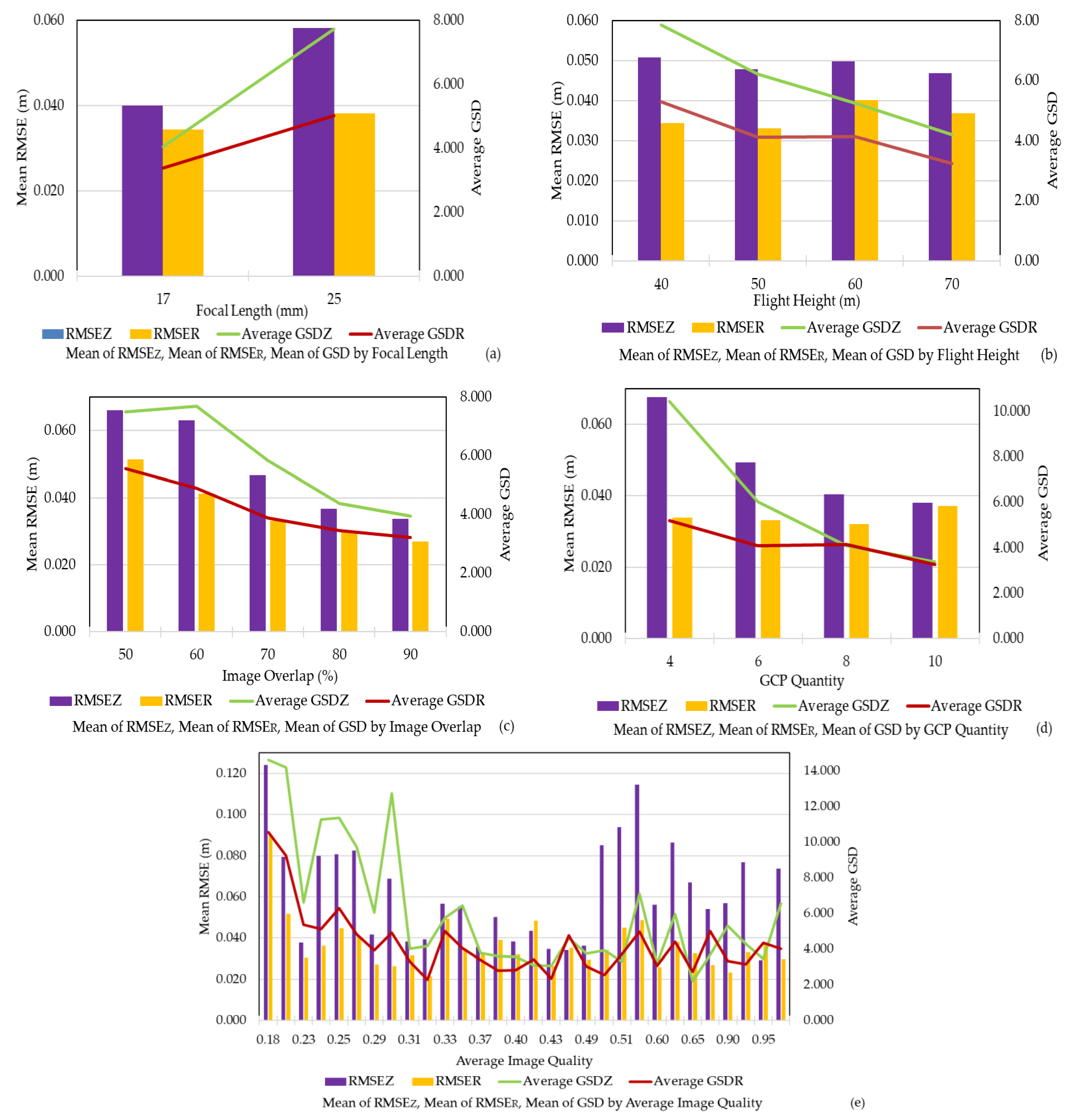
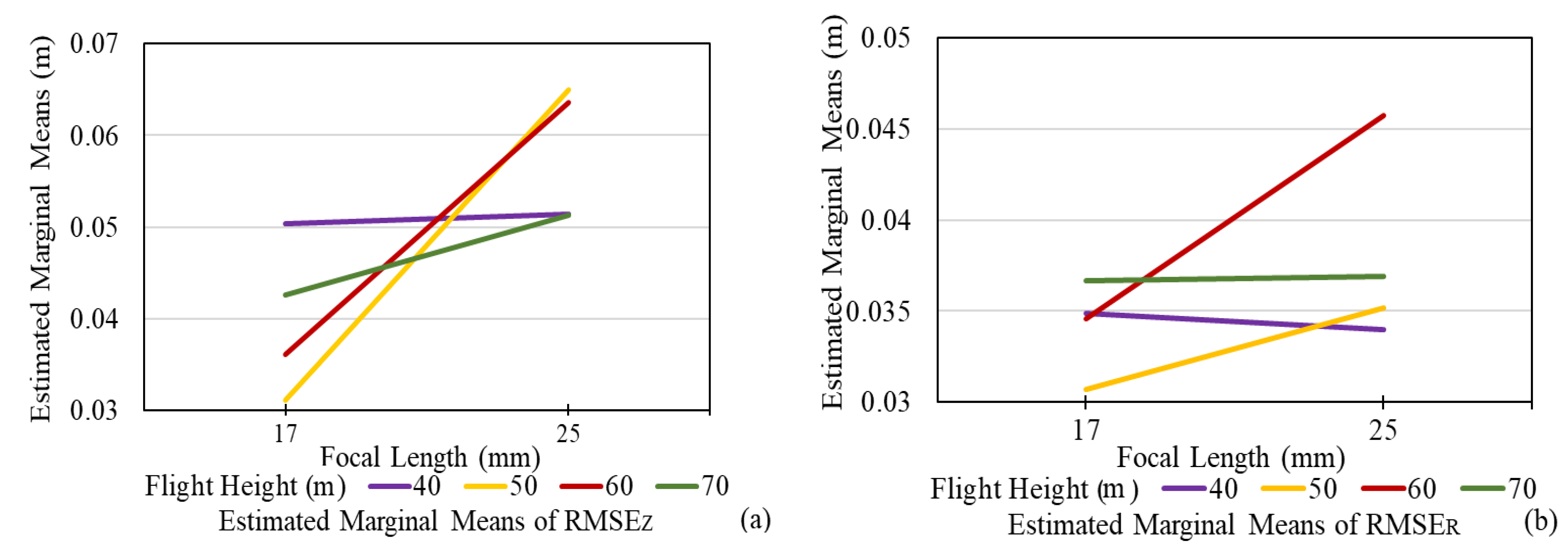
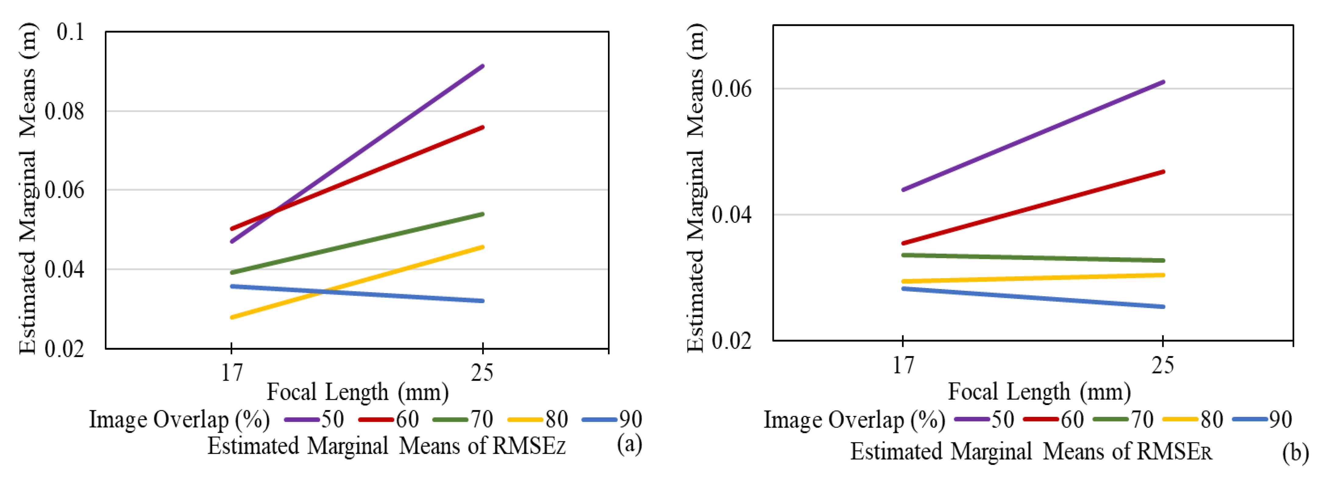
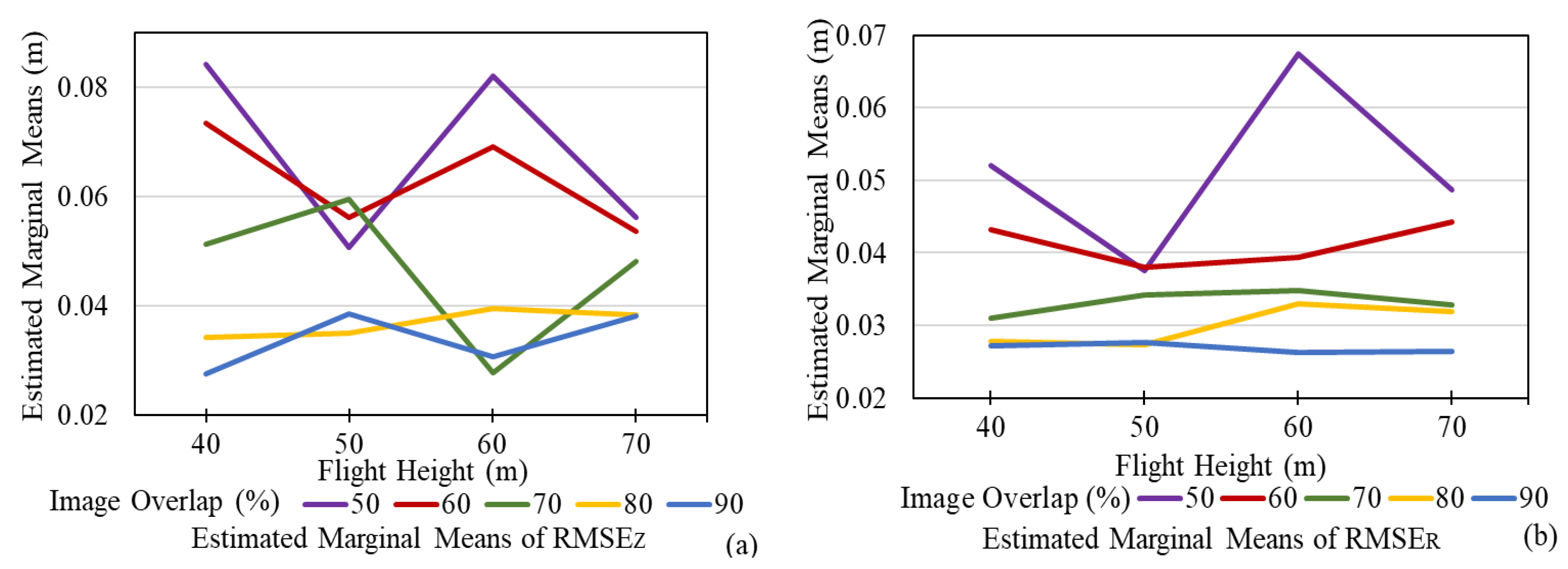
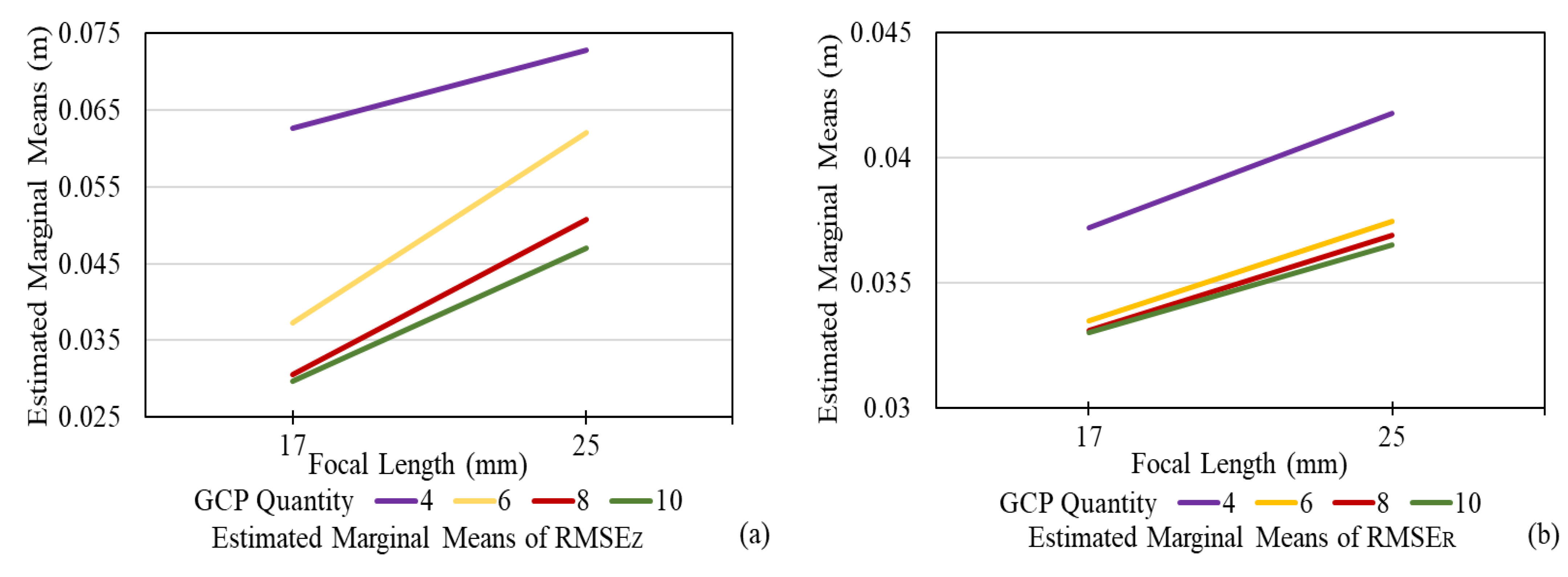
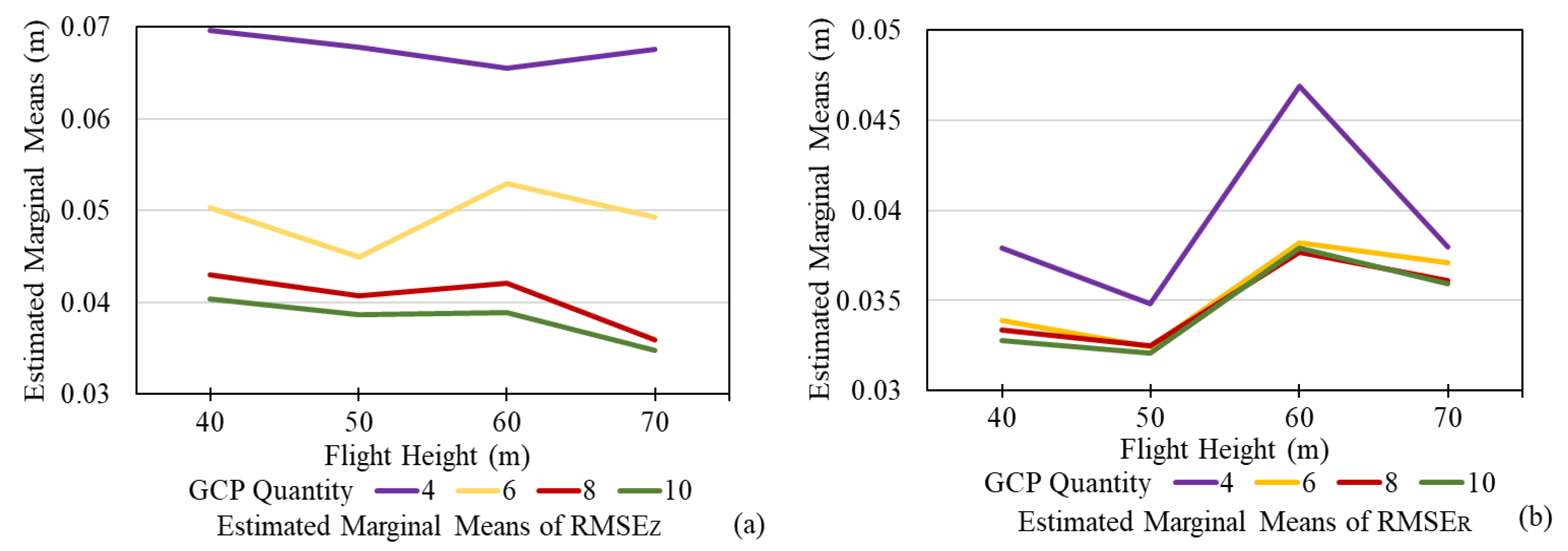
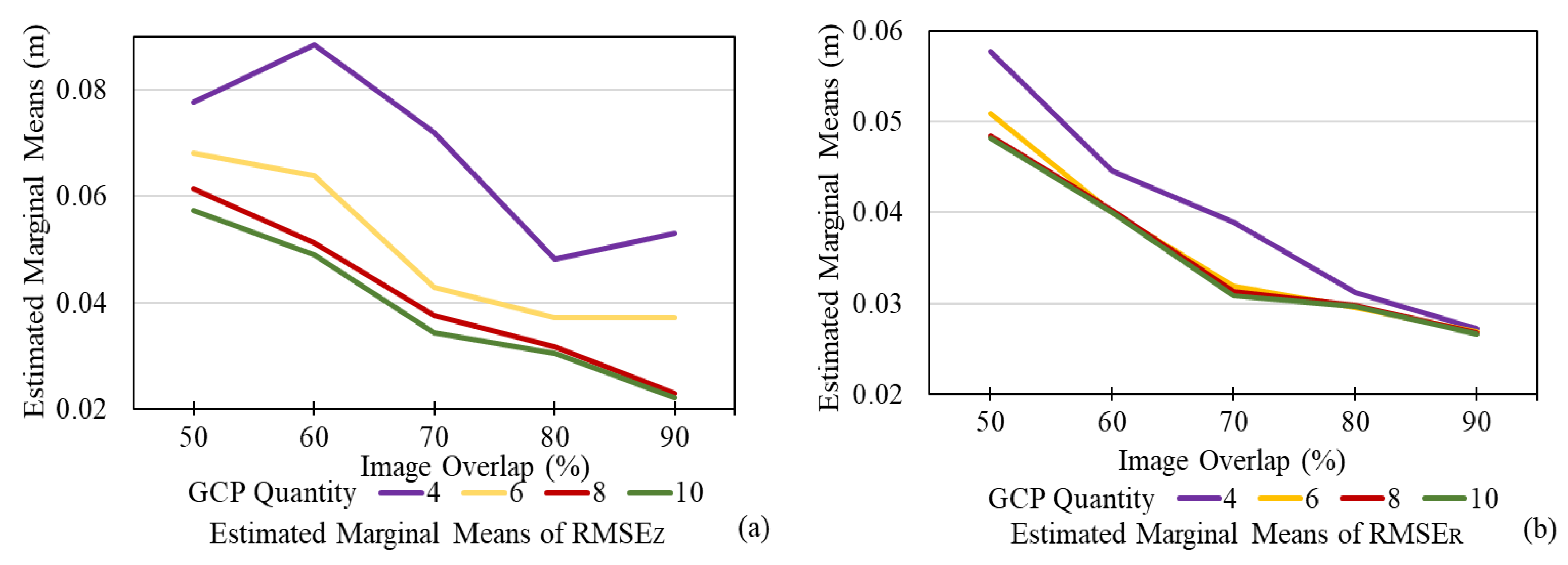
4.1. Influence and Significance of Five Influence Factors

This section summarizes the results of the aforementioned analysis and analyzes the impact of influence factors and their level of significance. Figure 9 shows the mean of RMSE_Z, RMSE_R, average errors in pixels in the horizontal direction (average GSDR), and average errors in pixels in the vertical direction (average GSDZ) for the five influence factors. Average GSD was calculated through divided the mean RSME in (m) by average GSD. As can be seen in the subfigures for all influence factors, the mean of RMSE_Z and average GSDZ are more sensitive to changes in influence factors than the mean of RMSE_R and average GSDR. In other words, the influence factors have a stronger influence on vertical accuracy than horizontal accuracy.

As shown in Figure 9a, the change in the focal length of the camera lens from 17 mm to 25 mm had a greater impact on the mean of RMSE_Z and average GSDZ than that of RMSE_R and average GSDR. Using a shorter focal length of the camera lens produced higher accuracies in both horizontal and vertical directions. Figure 9b shows that the mean of RMSE_R is more susceptible to the change in flight height than RMSE_Z. A lower flight height yielded a higher accuracy in the horizontal direction. However, a higher flight height yielded a high vertical accuracy.

As shown in Figure 9c,d, increasing the image overlap and the number of GCPs improved horizontal and vertical accuracies. However, there is no noticeable difference in RMSE_R using more than eight GCPs. Additionally, Figure 9e shows that the datasets with higher image qualities tend to yield higher accuracies in both directions, although there are some variations.

Table 6. Level of Significance of Influence Factors.

	p-Value for RMSEZ	p-Value for RMSER
Constant ${\beta }_0$	0.009	<0.001
Focal Length	0.773	0.057
Flight Height	0.438	0.367
Image Overlap	0.015	<0.001
GCP Quantity	0.027	0.126
Average Image Quality	0.427	0.103

below lists the p-values of the flight height, the focal length of lenses, image overlap, average image quality, and GCPs quantity for RMSE_Z and RMSE_R. The overlap and the GCP quantity have significant impacts with a 95% confidence level on RMSE_Z since the p-values are smaller than 0.05. Compared to other factors, the image overlap has a substantial impact with the 95% confidence level on RMSE_R since the p-values are smaller than 0.05. The focal length, flight height, and average image quality have a low significant influence on both RMSE_Z and RMSE_R. Both p-values of constant ${\beta }_0$ for RMSE_Z and RMSE_R are smaller than 0.05, which means it is essential to be included in the MR model to guarantee that the mean of residuals can be zero.

The following figures (Figure 10, Figure 11, Figure 12, Figure 13, Figure 14 and Figure 15) show the relationships between two influence factors with respect to RMSE_Z and RMSE_R. The X-axis shows the values of an influence factor. The Y-axis shows the values of estimated marginal means of the other influence factor. The estimated marginal mean represents the average response (RMSE values) of the influence factor on the Y-axis for each level of the influence factor on the X-axis.

As seen in the figures, there are interactions between influence factors since the estimated marginal means of RMSE_Z and RMSE_R for influence factors are not parallel. That means the impact of one influence factor on RMSE_Z and RMSE_R is affected by varying the other influence factor.

Figure 10 shows the interactions between the focal length and the flight height. It shows the influence of flight heights on accuracy when varying focal lengths. As seen in the figure, the accuracy of middle heights (50 m and 60 m flight heights) has the highest slope and, therefore, are more likely to be affected by changes in focal length.

Figure 11 shows the interactions between focal length and image overlap in horizontal and vertical directions. Compared to the high image overlap, such as 90% (lowest slope), the accuracy of the low image overlaps is more sensitive to change in focal length, especially for the 50% (highest slope) image overlap.

Figure 12 describes the interactions between flight height and image overlap. Similar to the results from Figure 11, the results show that low image overlap accuracy is more easily impacted by varying flight heights, especially for 50% image overlap. When the image overlap was high (i.e., 80% and 90%), the influence was relatively small, which indicates that successful feature detection and matching due to high image overlap ensures good quality 3D reconstruction and is less affected by flight heights.

Figure 13 shows the interactions between focal length and GCP quantity. Generally, a short focal length can produce high horizontal and vertical accuracy. As can be seen from the figures, the slopes except for four GCPs for RMSE_z are very similar, which indicates that the influence of change in focal length on different quantities of GCPs is not notably different.

Figure 14 shows the interactions between flight height and GCP. As can be seen in Figure 14a, the influence is more significant when six GCPs were used. Figure 14b shows that the influence is more significant with four GCPs. In both cases, with eight and ten GCPs, there was a relatively lower influence.

Figure 15 shows the interactions between image overlap and GCP quantity. The accuracy of using a low quantity of GCPs (e.g., 4 GCPs) is more susceptible to change in image overlap. Additionally, increasing both GCP quantity and image overlap decreases the vertical and horizontal errors.

According to the above results, higher accuracy can be expected when using a high image overlap (e.g., 80% or 90%) and a high number of GCPs (e.g., more than eight). The GCP quantity and image overlap had higher level of significances than other influence factors. However, even with a low GCP quantity and image overlap are used due to undesired data collection circumstances (i.e., limited time or battery), good values of other influence factors can significantly help improve accuracy.

In addition to identifying the relationship between dependent and independent variables and independent variables, MR models can be used to estimate dependent variables based on independent variables. Moreover, this MR model can be extended to predict the accuracy that can be achieved given a set of influence factors and site constraints. Thus, the following section introduces the development and validation of the MR prediction model.

4.2. MR Prediction Model Development and Validation

This section focuses on an MR model development using the five influence factors for the prediction of accuracies and validation.

4.2.1. MR Model Development

The distributions of RMSE_Z and RMSE_R of the 160 flight combinations are right-skewed (the values of skewness of RMSE_Z and RMSE_R are 0.918 and 2.801, respectively). To improve the MR prediction model fitness, the distributions of RMSE_Z and RMSE_R need to be transformed to normal distributions, which can be performed by applying a logarithmic transformation. The following equations show the logarithmic transformation:

$${\mathrm{lgRMSE}}_{\mathrm{z}}=\lg \left({\mathrm{RMSE}}_{\mathrm{Z}}\right)$$

(7)

$${\mathrm{lgRMSE}}_{\mathrm{R}}=\lg \left({\mathrm{RMSE}}_{\mathrm{R}}\right)$$

(8)

After transformation, the skewness of the distribution of the value of lgRMSE_Z and lgRMSE_R are −0.024 and 1.098, separately, which means the new distributions are closer to a normal distribution. Thus, the MR prediction models are established using the values of lgRMSE_Z, lgRMSE_R, influence factors, and the interactions between the influence factors. By plugging these values into Equations (5) and (6), the following MR prediction models are developed for vertical and horizontal directions ($y_z$ and $y_r$):

$$\begin{array}{l}{y}_z=-4.234+0.161\times x_{i1}+0.017\times x_{i2}+0.022\times x_{i3}+0.025\times x_{i4}+2.399\times x_{i5}\\ \hspace{1em}\hspace{1em}\hspace{1em}\hspace{1em}\hspace{1em}\hspace{1em}\hspace{1em}-0.001\times x_{i1}\times x_{i2}-0.001\times x_{i1}\times x_{i3}-0.049\times x_{i1}\times x_{i5}\\ \hspace{1em}\hspace{1em}\hspace{1em}\hspace{1em}\hspace{1em}\hspace{1em}\hspace{1em}+6.609\times {10}^{-5}\times x_{i2}\times x_{i3}-0.014\times x_{i2}\times x_{i5}-0.001\times x_{i3}\times x_{i4}\\ \hspace{1em}\hspace{1em}\hspace{1em}\hspace{1em}\hspace{1em}\hspace{1em}\hspace{1em}-0.011\times x_{i3}\times x_{i5}+0.003\times x_{i4}\times x_{i5}\end{array}$$

(9)

$$\begin{array}{l}{y}_z=-1.353+0.027\times x_{i1}-0.003\times x_{i3}-0.021\times x_{i4}-0.387\times x_{i5}\\ \hspace{1em}\hspace{1em}\hspace{1em}\hspace{1em}\hspace{1em}\hspace{1em}\hspace{1em}-4.066\times {10}^{-5}\times x_{i1}\times x_{i2}-0.001\times x_{i1}\times x_{i5}\\ \hspace{1em}\hspace{1em}\hspace{1em}\hspace{1em}\hspace{1em}\hspace{1em}\hspace{1em}-4.549\times {10}^{-5}\times x_{i2}\times x_{i3}+5.933\times {10}^{-5}\times x_{i2}\times x_{i4}\\ \hspace{1em}\hspace{1em}\hspace{1em}\hspace{1em}\hspace{1em}\hspace{1em}\hspace{1em}+0.005\times x_{i3}\times x_{i5}-0.011\times x_{i4}\times x_{i5}\end{array}$$

(10)

where $y_Z$ is the estimated value of lgRMSE_Z, $y_{ZR}$ is the estimated value of lgRMSE_R. $x_{i1}$ is the value of focal length; $x_{i2}$ is the value of flight height; $x_{i3}$ is the value of image overlap; $x_{i4}$ is the value of the GCP quantity; and $x_{i5}$ is the value of average image quality. –4.234 and –1.353 are the constant (${\beta }_0$ of the MR prediction models). The rest of the constants are the parameters (${\beta }_m$) of influence factors.

4.2.2. MR Prediction Models Applied to Test Site

The values of influence factors from the test site are imported into the MR prediction models (Equations (9) and (10)) to produce the predicted lgRMSE_Z and lgRMZE_R for flight missions 1 and 2. The predicted lgRMSE_Z and lgRMZE_R for flight mission 1 are −2.753 and −1.577, respectively. The predicted lgRMSE_Z and lgRMZE_R for flight mission 2 are −1.534 and −1.643, respectively. Then, an exponential function with the base of 10 is used to convert the values of predicted lgRMSE_Z and lgRMZE_R to the values of predicted RMSE_Z and predicted RMSE_R. The following are the exponential function for predicted RMSE_Z and predicted RMSE_R.

$${\mathrm{RMSE}}_{\mathrm{z}}={10}^{{\mathrm{lgRMSE}}_{Z }}$$

(11)

$${\mathrm{RMSE}}_{\mathrm{R}}={10}^{{\mathrm{lgRMSE}}_{R }}$$

(12)

Table 7. Results of Butner UAS Test Site from Pix4DMapper and MR Models.

Flight Mission	RMSEZ from Pix4D (cm)	Z Direction Pixel Error from Pix4D	RMSER from Pix4D (cm)	R Direction Pixel Error from Pix4D	Predicted RMSEZ from MR Model (cm)	Predicted Z Direction Pixel Error from MR Model	Predicted RMSER from MR Model (cm)	Predicted R Direction Pixel Error from MR Model
1	2.1	1.27 GSD	2.4	1.50 GSD	1.8	1.13 GSD	2.6	1.63 GSD
2	2.1	1.27 GSD	2.5	1.52 GSD	2.9	1.76 GSD	2.3	1.39 GSD
3	2.7	1.69 GSD	2.9	1.81 GSD	2.6	1.63 GSD	3.1	1.94 GSD
4	3.2	1.94 GSD	3.1	1.88 GSD	3.4	2.06 GSD	2.6	1.58 GSD
5	3.5	2.12 GSD	3.3	2.00 GSD	3.0	1.82 GSD	2.8	1.70 GSD

shows the validation results using these two MR prediction models with the data collected from the Butner UAS Test site. The differences between RMSE_Z from Pix4DMapper and the predicted RMSE_Z from the MR model for all flight missions are 0.3 cm and 0.7 cm, respectively. The differences between RMSE_R from Pix4DMapper and predicted RMSE_R from the MR model for all flight missions are from 0.2 cm to 0.5 cm. The differences between pixel error in the Z direction from Pix4DMapper and predicted MR model for all flight missions are 0.06 GSD and 0.49 GSD, respectively. The differences between pixel error in the R direction from Pix4DMapper and the predicted MR model for all flights are from 0.13 GSD to 0.3 GSD.

Table 8. Prediction Error Rate and Accuracy of Butner UAS Test Site from Pix4D and MR Models.

RMSEZ Error Rate	RMSER Error Rate	Prediction Accuracy	Prediction Accuracy
16.67	7.69	83.33	92.31
27.59	8.70	72.41	91.30
3.70	6.90	96.3	93.1
6.25	16.13	93.75	83.87
14.29	15.15	85.71	84.85

shows the Prediction Error Rate and Accuracy of the Butner UAS Test Site from Pix4DMapper and MR Models. The error rates of the RMSE_Z are 16.67% and 27.59%, which leads to the prediction accuracies of the MR prediction model being 72.41% and 83.33%, respectively. The MR prediction model has a lower error rate when estimating horizontal accuracy. The error rates of the RMSE_Z are 7.69% and 8.7%, and the prediction accuracies of the MR prediction model are 92.31% and 91.30%, respectively. The following equations show the error rate and prediction accuracy.

$$Error Rate=\frac{\left|\mathrm{Predicted} \mathrm{Values}-\mathrm{Actual} \mathrm{Values}\right|}{\mathrm{Actual} \mathrm{Values}}\times 100$$

(13)

$$\mathrm{Prediction\; Accuracy}=100\%-\mathrm{Error}\mathrm{Rate}$$

(14)

Thus, there are at least 72% and 83% prediction accuracy to predict the vertical and horizontal accuracies using five influence factors. Since the actual results from Pix4D can be influenced by other influence factors, such as wind speed and lighting environment, the current MR prediction models are sufficient to estimate the vertical and horizontal accuracies.

4.3. Practical Implications

Applying the findings of this research in practice can help surveyors better design flight missions based on the site constraints and conditions. For example, the typical flight time for most high-quality UAS is about 20 min. However, using a low flight height (for example, 40 m) on a large site for surveying will significantly increase the surveying time (for example, an hour) and, therefore, increase the number of batteries (for example, 5 or more sets of batteries) to be used. In this case, a high flight height (for example, 100 m) with a high image overlap (for example, 80 or 90%) can be applied to reduce the flight mission time (for example, 40 min). If higher accuracy is desired, the drone speed can be increased as long as the camera can capture good quality images while maintaining the high image overlap. Surveyors can use the MR prediction model to predict what combination of the influence factors given these alternative situations to optimize their workflow while achieving the desired accuracy.

Additionally, the MR prediction model can be applied to repeated similar scenarios, such as construction progress monitoring. For agencies such as the state Department of Transportation (DOTs), surveyors can build their own model with very similar scenarios with the same set of hardware and software used over and over. However, the MR model cannot be generalized for all the scenarios, such as the scenarios that required categorical data as input variables. It can be generalized to a certain degree if the users include all variations of scenarios for their use cases. In this case, surveyors can build their own MR model for their own use cases using a set of equipment on certain terrain types of interest.

4.4. Limitations and Future Work

There are a few limitations of this research. First, the MR model in this paper is developed using one terrain type—a facility with an open field. Therefore, MR models for different types of terrains (i.e., vertical surfaces, excavation sites, etc.) and more scenarios should be either included in the training or separately trained and separately used for prediction, which will be the authors’ future work.

Moreover, regarding the selection of the validation site, the site is relatively flat, which means the CPs appear at the same height as the GCPs. It may cause a high correlation and yield inaccurate results. Thus, more sites with elevation differences should be selected in future work to reduce the correlation.

Additionally, although five influence factors are used in this research, more influence factors (e.g., camera calibration and weather conditions) can be identified and used to create a more accurate MR prediction model, which can be used in general cases. Any practitioners who want to implement the presented method, will have to build their own model using the set of influence factors that are specific to the set of hardware they own.

Additionally, since MR analysis is based on hypothesis testing, there is some prerequisite before applying the MR, including linear relationship, multivariate normality, no or little multicollinearity, no auto-correlation, and homoscedasticity. This method may not fit other data with complex terrains and different devices. Thus, the users could consider another statistical method that is the most suitable for their cases, such as using an alternative method that contains flight planning with simulations.

Lastly, in this research, a multirotor drone is used. Multirotor drones rely on the spinning of their rotors to stay stable in the air, making them vulnerable to high wind. Thus, the image with low quality may be captured during windy weather. In addition, there are restrictions on the altitude most standard multirotor drones can fly at since the drone needs air to stay airborne by spinning the rotors and generating enough lift. Thus, it is necessary to consider the drone according to the flight height and wind speed.

5. Conclusions

A combination of computer vision, photogrammetry, and remote sensing techniques provide the camera-equipped UAS yielding a highly accurate point cloud model on UAS-based photogrammetric surveying. However, the accuracy of this point cloud model can be influenced by many factors. Although there have been many studies on various factors that affect the accuracy of such data, most previous studies focus on the influence on accuracy caused by image overlaps, GCP quantity, and GNSS types. Little research studies the effect of other influence factors on the accuracy using quantitative methods to identify the relationships between flight configuration influence factors and point cloud accuracy. This paper evaluated the levels of significance of five influence factors on accuracy using an MR method. The influence factors include flight height, average image quality, image overlap, GCP quantity, and focal lengths of cameras. 40 flight missions were conducted using different flight configurations at the track facility site. 160 datasets were processed using all conducted flight missions with four different numbers of GCPs.

The results show that image overlap is highly significant to the vertical and horizontal accuracies of all the influence factors. The quantity of GCPs has high significance on vertical accuracy. The rest of the influence factors have low levels of significance on both horizontal and vertical accuracies. In addition, this research shows that there are interactions between two influence factors. The impact of one influence factor on accuracy can be affected by changing the values of another influence factor. Thus, a lower accuracy can be generated using a smaller number of GCPs and a lower image overlap.

Additionally, two MR prediction models were developed to estimate the value of RMSE_Z and RMSE_R based on site conditions on a facility site. Moreover, the developed MR prediction models were validated using other datasets collected from the Butner site with s similar terrain type. The validation result shows the difference in the accuracy between MR prediction models and Pix4DMapper is less than 0.007 m, which proves the MR prediction models can be used to estimate the horizontal and vertical accuracies based on flight configurations and site conditions at a facility site with open space at a 72% prediction accuracy. The findings of this study can help surveyors better design flight configurations given different site conditions and constraints. Furthermore, the findings of this research can provide a basic understanding of what levels of accuracy could be achieved using different flight configurations. Moreover, agencies such as state DOTs can generate their prediction models based on their data and sets of equipment used on the interesting sites using our proposed method, especially on some repeated similar scenarios, such as construction progress monitoring.

Since the MR models in this paper were developed using a single type of terrain with five influence factors, in future work, more types of terrains and influence factors will be included to generalize the findings in different scenarios.

References

1. Gabrlik, P.; la Cour-Harbo, A.; Kalvodova, P.; Zalud, L.; Janata, P. Calibration and Accuracy Assessment in a Direct Georeferencing System for UAS Photogrammetry. Int. J. Remote Sens. 2018, 39, 4931–4959. [Google Scholar] [CrossRef] [Green Version]
2. Benjamin, A.R.; O’Brien, D.; Barnes, G.; Wilkinson, B.E.; Volkmann, W. Improving Data Acquisition Efficiency: Systematic Accuracy Evaluation of GNSS-Assisted Aerial Triangulation in UAS Operations. J. Surv. Eng. 2020, 146, 05019006. [Google Scholar] [CrossRef]
3. Raeva, P.L.; Šedina, J.; Dlesk, A. Monitoring of Crop Fields Using Multispectral and Thermal Imagery from UAV. Eur. J. Remote Sens. 2019, 52, 192–201. [Google Scholar] [CrossRef] [Green Version]
4. Hoffmann, H.; Nieto, H.; Jensen, R.; Guzinski, R.; Zarco-Tejada, P.; Friborg, T. Estimating Evaporation with Thermal UAV Data and Two-source Energy Balance Models. Hydrol. Earth Syst. Sci. 2016, 20, 697–713. [Google Scholar] [CrossRef] [Green Version]
5. Guo, Y.; Senthilnath, J.; Wu, W.; Zhang, X.; Zeng, Z.; Huang, H. Radiometric Calibration for Multispectral Camera of Different Imaging Conditions Mounted on a UAV Platform. Sustainability 2019, 11, 978. [Google Scholar] [CrossRef] [Green Version]
6. Navia, J.; Mondragon, I.; Patino, D.; Colorado, J. Multispectral Mapping in Agriculture: Terrain Mosaic Using an Autonomous Quadcopter UAV. In Proceedings of the 2016 International Conference on Unmanned Aircraft Systems, Arlington, VA, USA, 7–10 June 2016; pp. 1351–1358. [Google Scholar] [CrossRef]
7. Lin, Y.C.; Cheng, Y.T.; Zhou, T.; Ravi, R.; Hasheminasab, S.; Flatt, J.; Troy, C.; Habib, A. Evaluation of UAV LiDAR for Mapping Coastal Environments. Remote Sens. 2019, 11, 2893. [Google Scholar] [CrossRef] [Green Version]
8. Elaksher, A.F.; Bhandari, S.; Carreon-Limones, C.A.; Lauf, R. Potential of UAV lidar systems for geospatial mapping. In Proceedings of the Lidar Remote Sensing for Environmental Monitoring, San Diego, CA, USA, 8–9 August 2017; Volume 10406, pp. 121–133. [Google Scholar] [CrossRef]
9. Nex, F.; Armenakis, C.; Cramer, M.; Cucci, D.A.; Gerke, M.; Honkavaara, E.; Kukko, A.; Persello, C.; Skaloudh, J. UAV in the Advent of the Twenties: Where We Stand and What is Next. ISPRS J. Photogramm. Remote Sens. 2022, 184, 215–242. [Google Scholar] [CrossRef]
10. Ruzgiene, B.; Berteška, T.; Gečyte, S.; Jakubauskiene, E.; Aksamitauskas, V.Č. The Surface Modelling based on UAV Photogrammetry and Qualitative Estimation. Meas. J. Int. Meas. Confed. 2015, 73, 619–627. [Google Scholar] [CrossRef]
11. Seifert, E.; Seifert, S.; Vogt, H.; Drew, D.; Van Aardt, J.; Kunneke, A.; Seifert, T. Influence of Drone Altitude, Image Overlap, and Optical Sensor Resolution on Multi-view Reconstruction of Forest Images. Remote Sens. 2019, 11, 1252. [Google Scholar] [CrossRef] [Green Version]
12. Gerke, M.; Przybilla, H.J. Accuracy Analysis of Photogrammetric UAV Image Blocks: Influence of Onboard RTK-GNSS and Cross Flight Patterns. Photogramm. Fernerkund. Geoinf. 2016, 2016, 17–30. [Google Scholar] [CrossRef] [Green Version]
13. Ajayi, O.G.; Palmer, M.; Salubi, A.A. Modelling Farmland Topography for Suitable Site Selection of Dam Construction Using Unmanned Aerial Vehicle (UAV) Photogrammetry. Remote Sens. Appl. Soc. Environ. 2018, 11, 220–230. [Google Scholar] [CrossRef]
14. Catania, P.; Comparetti, A.; Febo, P.; Morello, G.; Orlando, S.; Roma, E.; Vallone, M. Positioning Accuracy Comparison of GNSS Receivers Used for Mapping and Guidance of Agricultural Machines. Agronomy 2020, 10, 924. [Google Scholar] [CrossRef]
15. Padró, J.C.; Muñoz, F.J.; Planas, J.; Pons, X. Comparison of Four UAV Georeferencing Methods for Environmental Monitoring Purposes Focusing on the Combined Use with Airborne and Satellite Remote Sensing Platforms. Int. J. Appl. Earth Obs. Geoinf. 2019, 75, 130–140. [Google Scholar] [CrossRef]
16. Shenbagaraj, N.; kumar, K.S.; Rasheed, A.M.; Leostalin, J.; Kumar, M.N. Mapping and Electronic Publishing of Shoreline Changes using UAV Remote Sensing and GIS. J. Indian Soc. Remote Sens. 2021, 49, 1769–1777. [Google Scholar] [CrossRef]
17. Hemmelder, S.; Marra, W.; Markies, H.; de Jong, S.M. Monitoring River Morphology & Bank Erosion Using UAV Imagery—A Case study of the River Buëch, Hautes-Alpes, France. Int. J. Appl. Earth Obs. Geoinf. 2018, 73, 428–437. [Google Scholar] [CrossRef]
18. Koucká, L.; Kopačková, V.; Fárová, K.; Gojda, M. UAV Mapping of an Archaeological Site Using RGB and NIR High-Resolution Data. Proceedings 2018, 2, 351. [Google Scholar] [CrossRef] [Green Version]
19. arba, S.; Barbarella, M.; di Benedetto, A.; Fiani, M.; Gujski, L.; Limongiello, M. Accuracy Assessment of 3D Photogrammetric Models from an Unmanned Aerial Vehicle. Drones 2019, 3, 79. [Google Scholar] [CrossRef] [Green Version]
20. Karachaliou, E.; Georgiou, E.; Psaltis, D.; Stylianidis, E. UAV for Mapping Historic Buildings: From 3D Modling to BIM. ISPRS Ann. Photogramm. Remote Sens. Spat. Inf. Sci. 2019, 42, 397–402. [Google Scholar] [CrossRef] [Green Version]
21. Zulkipli, M.A.; Tahar, K.N. Multirotor UAV-Based Photogrammetric Mapping for Road Design. Int. J. Opt. 2018, 2018, 1871058. [Google Scholar] [CrossRef]
22. Hubbard, B.; Hubbard, S. Unmanned Aircraft Systems (UAS) for Bridge Inspection Safety. Drones 2020, 4, 40. [Google Scholar] [CrossRef]
23. Chen, S.; Laefer, D.F.; Mangina, E.; Zolanvari, S.M.I.; Byrne, J. UAV Bridge Inspection through Evaluated 3D Reconstructions. J. Bridge Eng. 2019, 24, 05019001. [Google Scholar] [CrossRef] [Green Version]
24. Stampa, M.; Sutorma, A.; Jahn, U.; Willich, F.; Pratzler-Wanczura, S.; Thiem, J.; Röhrig, C.; Wolff, C. A Scenario for a Multi-UAV Mapping and Surveillance System in Emergency Response Applications. In Proceedings of the IDAACS-SWS 2020—5th IEEE International Symposium on Smart and Wireless Systems within the International Conferences on Intelligent Data Acquisition and Advanced Computing Systems, Dortmund, Germany, 17–18 September 2020. [Google Scholar] [CrossRef]
25. Snavely, N.; Seitz, M.; Szeliski, R. Modeling the World from Internet Photo Collections. Int. J. Comput. Vis. 2007, 80, 189–210. [Google Scholar] [CrossRef] [Green Version]
26. Förstner, W.; Wrobel, B.P. Photogrammetric Computer Vision Statistics, Geometry, Orientation and Reconstruction; Springer International Publishing: Cham, Switzerland, 2016; Volume 11. [Google Scholar] [CrossRef] [Green Version]
27. Anders, N.; Smith, M.; Suomalainen, J.; Cammeraat, E.; Valente, J.; Keesstra, S. Impact of Flight Altitude and Cover Orientation on Digital Surface Model (DSM) Accuracy for Flood Damage Assessment in Murcia (Spain) Using a Fixed-Wing UAV. Earth Sci. Inform. 2020, 13, 391–404. [Google Scholar] [CrossRef] [Green Version]
28. Agüera-Vega, F.; Carvajal-Ramírez, F.; Martínez-Carricondo, P. Accuracy of Digital Surface Models and Orthophotos Derived from Unmanned Aerial Vehicle Photogrammetry. J. Surv. Eng. 2017, 143, 04016025. [Google Scholar] [CrossRef]
29. Zhang, D.; Watson, R.; Dobie, G.; MacLeod, C.; Khan, A.; Pierce, G. Quantifying Impacts on Remote Photogrammetric Inspection Using Unmanned Aerial Vehicles. Eng. Struct. 2020, 209, 109940. [Google Scholar] [CrossRef]
30. Fraser, B.T.; Congalton, R.G. Issues in Unmanned Aerial Systems (UAS) Data Collection of Complex Forest Environments. Remote Sens. 2018, 10, 908. [Google Scholar] [CrossRef] [Green Version]
31. Domingo, D.; Ørka, H.O.; Næsset, E.; Kachamba, D.; Gobakken, T. Effects of UAV Image Resolution, Camera Type, and Image Overlap on Accuracy of Biomass Predictions in a Tropical Woodland. Remote Sens. 2019, 11, 948. [Google Scholar] [CrossRef] [Green Version]
32. Burdziakowski, P.; Bobkowska, K. UAV Photogrammetry under Poor Lighting Conditions—Accuracy Considerations. Sensors 2021, 21, 3531. [Google Scholar] [CrossRef]
33. Taddia, Y.; Stecchi, F.; Pellegrinelli, A. Coastal Mapping Using DJI Phantom 4 RTK in Post-Processing Kinematic Mode. Drones 2020, 4, 9. [Google Scholar] [CrossRef] [Green Version]
34. Toth, C.; Jozkow, G.; Grejner-Brzezinska, D. Mapping with Small UAS: A Point Cloud Accuracy Assessment. J. Appl. Geod. 2015, 9, 213–226. [Google Scholar] [CrossRef]
35. Tomaštík, J.; Mokroš, M.; Saloš, S.; Chudỳ, F.; Tunák, D. Accuracy of Photogrammetric UAV-based Point Clouds under Conditions of Partially-Open Forest Canopy. Forests 2017, 8, 151. [Google Scholar] [CrossRef] [Green Version]
36. Han, K.; Rasdorf, W.; Liu, Y. Applying Small UAS to Produce Survey Grade Geospatial Products for DOT Preconstruction & Construction. 2021. Available online: https://connect.ncdot.gov/projects/research/Pages/ProjDetails.aspx?ProjectID=2020-18 (accessed on 1 March 2022).
37. American Society for Photogrammetry and Remote Sensing (ASPRS). ASPRS Positional Accuracy Standards for Digital Geospatial Data. Photogramm. Eng. Remote Sens. 2015, 81, A1–A26. [Google Scholar] [CrossRef]
38. Ferrer-González, E.; Agüera-Vega, F.; Carvajal-Ramírez, F.; Martínez-Carricondo, P. UAV Photogrammetry Accuracy Assessment for Corridor Mping based on the Number and Distribution of Ground Control Points. Remote Sens. 2020, 12, 2447. [Google Scholar] [CrossRef]
39. Gindraux, S.; Boesch, R.; Farinotti, D. Accuracy Assessment of Digital Surface Models from Unmanned Aerial Vehicles’ Imagery on Glaciers. Remote Sens. 2017, 9, 186. [Google Scholar] [CrossRef] [Green Version]
40. Martínez-Carricondo, P.; Agüera-Vega, F.; Carvajal-Ramírez, F.; Mesas-Carrascosa, F.J.; García-Ferrer, A.; Pérez-Porras, F.J. Assessment of UAV-Photogrammetric Mapping Accuracy based on Variation of Ground Gontrol Points. Int. J. Appl. Earth Obs. Geoinf. 2018, 72, 1–10. [Google Scholar] [CrossRef]
41. Oniga, E.’; Breaban, A.; Statescu, F. Determining the Optimum Number of Ground Control Points for Obtaining High Precision Results based on UAS Images. Multidiscip. Digit. Publ. Inst. Proc. 2018, 2, 5165. [Google Scholar] [CrossRef] [Green Version]
42. Ridolfi, E.; Buffi, G.; Venturi, S.; Manciola, P. Accuracy Analysis of a Dam Model from Drone Surveys. Sensors 2017, 17, 1777. [Google Scholar] [CrossRef] [Green Version]
43. Sanz-Ablanedo, E.; Chandler, J.H.; Rodríguez-Pérez, J.R.; Ordóñez, C. Accuracy of Unmanned Aerial Vehicle (UAV) and SfM Photogrammetry Survey as a Function of the Number and Location of Ground Control Points Used. Remote Sens. 2018, 10, 1606. [Google Scholar] [CrossRef] [Green Version]
44. Stott, E.; Williams, R.D.; Hoey, T.B. Ground Control Point Distribution for Accurate Kilometre-scale Topographic Mapping using an RTK-GNSS Unmanned Aerial Vehicle and SfM Photogrammetry. Drones 2020, 4, 55. [Google Scholar] [CrossRef]
45. Yu, J.J.; Kim, W.E.; Lee, J.; Son, S.W. Determining the Optimal Number of Ground Control Points for Varying Study Sites through Accuracy Evaluation of Unmanned Aerial System-based 3D Point Clouds and Digital Surface Model. Drones 2020, 4, 49. [Google Scholar] [CrossRef]
46. James, M.R.; Robson, S.; d’Oleire-Oltmanns, S.; Niethammer, U. Optimising UAV Topographic Surveys Processed with Structure-from-Motion: Ground Control Quality, Quantity and Bundle Adjustment. Geomorphology 2017, 280, 51–66. [Google Scholar] [CrossRef] [Green Version]
47. Wierzbicki, D. Multi-camera Imaging System for UAV Photogrammetry. Sensors 2018, 18, 2433. [Google Scholar] [CrossRef] [PubMed] [Green Version]
48. Zhou, Y.; Rupnik, E.; Faure, P.H.; Pierrot-Deseilligny, M. GNSS-assisted Integrated Sensor Orientation with Sensor Pre-calibration for Accurate Corridor Mapping. Sensors 2018, 18, 2783. [Google Scholar] [CrossRef] [PubMed] [Green Version]
49. Alfio, V.S.; Costantino, D.; Pepe, M. Influence of Image TIFF Format and JPEG Compression Level in the Accuracy of the 3D Model and Auality of the Orthophoto in UAV Photogrammetry. J. Imaging 2020, 6, 30. [Google Scholar] [CrossRef]
50. Yang, Y.; Lin, Z.; and Liu, F. Stable Imaging and Accuracy Issues of Low-Altitude Unmanned Aerial Vehicle Photogrammetry Systems. Remote Sens. 2016, 8, 316. [Google Scholar] [CrossRef] [Green Version]
51. Benassi, F.; Dall’Asta, E.; Diotri, F.; Forlani, G.; Cella, U.; Roncella, R.; Santise, M. Testing Accuracy and Repeatability of UAV Blocks Oriented with GNSS-Supported Aerial Triangulation. Remote Sens. 2017, 9, 172. [Google Scholar] [CrossRef] [Green Version]
52. Jurjević, L.; Gašparović, M.; Milas, A.S.; Balenović, I. Impact of UAS Image Orientation on Accuracy of Forest Inventory Attributes. Remote Sens. 2020, 12, 404. [Google Scholar] [CrossRef] [Green Version]
53. Kalacska, M.; Lucanus, O.; Arroyo-Mora, J.P.; Laliberté, E.; Elmer, K.; Leblanc, G.; Groves, A. Accuracy of 3D Landscape Reconstruction without Ground Control Points Using Different UAS Platforms. Drones 2020, 4, 13. [Google Scholar] [CrossRef] [Green Version]
54. Losè, L.T.; Chiabrando, F.; Tonolo, F.G. Boosting the Timeliness of UAV Large Scale Mapping. Direct Georeferencing Approaches: Operational Strategies and Best Practices. ISPRS Int. J. Geo-Inf. 2020, 9, 578. [Google Scholar] [CrossRef]
55. Martinez, J.G.; Albeaino, G.; Gheisari, M.; Volkmann, W.; Alarcón, L.F. UAS Point Cloud Accuracy Assessment Using Structure from Motion–Based Photogrammetry and PPK Georeferencing Technique for Building Surveying Applications. J. Comput. Civ. Eng. 2020, 35, 05020004. [Google Scholar] [CrossRef]
56. Tomaštík, J.; Mokroš, M.; Surový, P.; Grznárová, A.; Merganič, J. UAV RTK/PPK Method-An Optimal Solution for Mapping Inaccessible Forested Areas? Remote Sens. 2019, 11, 721. [Google Scholar] [CrossRef] [Green Version]
57. Agüera-Vega, F.; Carvajal-Ramírez, F.; Martínez-Carricondo, P. Assessment of Photogrammetric Mapping Accuracy based on Variation Ground Control Points Number Using Unmanned Aerial Vehicle. Meas. J. Int. Meas. Confed. 2017, 98, 221–227. [Google Scholar] [CrossRef]
58. Lee, S.; Park, J.; Choi, E.; Kim, D. Factors Influencing the Accuracy of Shallow Snow Depth Measured Using UAV-based Photogrammetry. Remote Sens. 2021, 13, 828. [Google Scholar] [CrossRef]
59. Zimmerman, T.; Jansen, K.; Miller, J. Analysis of UAS Flight Altitude and Ground Control Point Parameters on DEM Accuracy along a Complex, Developed Coastline. Remote Sens. 2020, 12, 2305. [Google Scholar] [CrossRef]
60. Harwin, S.; Lucieer, A.; Osborn, J. The Impact of the Calibration Method on the Accuracy of Point Clouds Derived Using Unmanned Aerial Vehicle multi-view stereopsis. Remote Sens. 2015, 7, 11933–11953. [Google Scholar] [CrossRef] [Green Version]
61. Wang, X.; Chen, J.C.; Dadi, G.B. Factors Influencing Measurement Accuracy of Unmanned Aerial Systems (UAS) and Photogrammetry in Construction Earthwork. In Computing in Civil Engineering 2019: Data, Sensing, and Analytics; American Society of Civil Engineers: Reston, VA, USA, 2019; pp. 408–414. [Google Scholar] [CrossRef]
62. Griffiths, D.; Burningham, H. Comparison of Pre- and Self-Calibrated Camera Calibration Models for UAS-Derived Nadir Imagery for a SfM Application. Prog. Phys. Geog. 2019, 43, 215–235. [Google Scholar] [CrossRef] [Green Version]
63. Cledat, E.; Jospin, L.V.; Cucci, D.A.; Skaloud, J. Mapping Quality Prediction for RTK/PPK-equipped Micro-drones Operating in Complex Natural Environment. ISPRS J. Photogramm. Remote Sens. 2020, 167, 24–38. [Google Scholar] [CrossRef]
64. Unmanned Systems Technology. 2022. Available online: https://www.unmannedsystemstechnology.com/expo/uav-autopilot-systems/#:~:text=What%20is%20an%20UAV%20Autopilot%20Unit%3F (accessed on 14 August 2022).
65. Scan Accuracy Checks for the Focus—FARO® Knowledge Base. Available online: https://knowledge.faro.com/Hardware/3D_Scanners/Focus/Scan_Accuracy_Checks_for_the_Focus (accessed on 19 August 2021).
66. FARO® SCENE 3D Point Cloud Software | FARO. Available online: https://www.faro.com/en/Products/Software/SCENE-Software (accessed on 14 August 2022).
Figure 1. Workflow of Research Process: Methodology and Results Validation.
Remotesensing 14 04119 g001
Figure 2. Study Site Conditions.
Remotesensing 14 04119 g002
Figure 3. Layout of GCPs and CPs in NCSU track facility site.
Remotesensing 14 04119 g003
Figure 4. Checkerboard.
Remotesensing 14 04119 g004
Figure 5. DJI Inspire II UAS: (a) DJI Inspire II drone, (b) DJI Zenmuse X5S camera and an Olympus M.Zuiko lens.
Remotesensing 14 04119 g005
Figure 6. FARO Focus S 3D scanner.
Remotesensing 14 04119 g006
Figure 7. Butner Site Conditions (Flat surface with buildings, open spaces, and vegetation).
Remotesensing 14 04119 g007
Figure 8. Layout of GCPs and CPs in NCDOT UAS test site.
Remotesensing 14 04119 g008
Figure 9. Mean of RMSEZ, RMSER, and average GSD for Five Influence Factors: (a) Focal Length; (b) Flight Heights; (c) Image Overlaps; (d) GCP Quantities; and (e) Average Image Quality.
Remotesensing 14 04119 g009
Figure 10. Interaction between Focal Length and Flight Height; (a) RMSEZ; (b) RMSER.
Remotesensing 14 04119 g010
Figure 11. Interaction between Focal Length and Image Overlap; (a) RMSEZ; (b) RMSER.
Remotesensing 14 04119 g011
Figure 12. Interaction between Flight Height and Image Overlap; (a) RMSEZ; (b) RMSER.
Remotesensing 14 04119 g012
Figure 13. Interaction between Focal Length and GCP Quantity; (a) RMSEZ; (b) RMSER.
Remotesensing 14 04119 g013
Figure 14. Interaction between Flight Height and GCP Quantity; (a) RMSEZ; (b) RMSER.
Remotesensing 14 04119 g014
Figure 15. Interaction between Image Overlap and GCP Quantity; (a) RMSEZ; (b) RMSER.
Remotesensing 14 04119 g015