1. Introduction
According to the State of World Fisheries and Aquaculture report [
1], aquatic product output is expected to increase from 179 million tons in 2018 to 204 million tons in 2030. With the increase in population, the demand for seafood and damage to the ocean are increasing, which leads to the continuous decline of marine fishery resources. An effective way to alleviate this problem is to raise the proportion of marine pastures in the supply of aquatic products [
2], which can ensure the steady and sustainable growth of aquatic resources. Therefore, it is necessary to manage marine pastures scientifically and effectively. In recent years, the rapid development of submarine cable online observation systems has provided a way to systematically manage marine pastures. The quantity and behavior of marine organisms can be monitored and tracked using cameras and sensors in an observation system, promoting scientific fishery management and sustainable fish production [
3,
4,
5]. For example, we can obtain species diversity and richness through video detection and tracking, which can be applied to disease identification, hypoxia stress identification, etc. In addition, we can analyze the coupling relationship between environmental factors and marine organism populations [
6].
Fish detection and behavior analyses have been conducted in ocean observation, aquaculture, and biological research. Compared with the traditional method, fish-tracking methods based on computer vision are real-time and automatic, and the expected behaviors of fish are unaffected [
7]. However, underwater observation equipment is usually expensive, and difficult to deploy and maintain. Moreover, it is challenging to continuously access underwater videos in real time in the ocean. Research on underwater fish school detection and tracking is primarily performed in following three ways.
(1) Most studies are conducted using laboratory video observations [
8,
9,
10,
11,
12], and tanks are used to breed fish. They artificially change environmental variables to study underwater fish tracking algorithms and behaviors. Observing and researching a fish school in a flume is convenient. Still, it cannot simulate a complex natural marine or lake environment, such as with underwater color distortion and wave slamming. So, it is challenging to transfer laboratory algorithms to a natural underwater environment.
(2) Some studies use online open datasets, such as ImageNet [
13] and Fish4-Knowledge [
14]. These collections consist of discontinuous images extracted from different underwater videos, and limited fish species, behaviors, and environmental water conditions are included. Thus, these online open datasets are usually insufficient for a specific underwater fish-school detection and tracking study.
(3) Some studies use the underwater videos of cameras equipped on an underwater observation platform, such as cabled seafloor observatory systems [
15]. Underwater observation videos can be continuously transmitted to a land observation center in real time by using a submarine cable. Many data are available, and online detection and tracking algorithms can be applied to them. The videos used in this study are from an underwater observation platform.
A fish resource statistical technology usually consists of two key steps: first, the accurate underwater detection of fish, and then associating the detected fish in every frame with the tracklets. Current research on technical solutions can be generally grouped into three categories [
16].
The first approach uses traditional computer graphics algorithms, such as a background subtraction algorithm [
17] or a Gaussian mixture model [
18]. Each fish in the frames is matched in the video to obtain the trajectories. Matching methods are usually prediction models, such as the Kalman filter [
19] and particle filter [
20]. Recently, FlowTrack [
21], which is used for small-scale tracking, introduced an optical flow method by calculating the motion vectors of each pixel between frames that can apply to fish targets [
22]. However, it is complex and time-consuming, and its tracking performance relies heavily on the detection results. It showed poor performance in a turbid water environment due to noise such as water plants and rocks.
The second approach is a one-stage deep learning scheme that combines detection and tracking models into a unified framework, and can avoid the overall loss caused by submodel errors. The joint detection and embedding (JDE) model [
23] is the first algorithm based on this idea; later on, its successors, FairMOT [
24] and RMCF [
25], were also developed. However, these algorithms treat object identity as a classification task. In particular, all object instances of the same identity in a training set are treated as one class. The number of objects grows over time; thus, an increasing number of categories need to be classified, which deteriorates the algorithm’s performance. Moreover, it is difficult to associate the trajectories of those objects re-entering the camera view.
The third approach is the two-stage deep learning algorithm following the tracking-by-detection paradigm. It generally detects objects by first using a neural network and then associating objects using a filtering method or a reidentification algorithm. Detection algorithms include YOLOx [
26], Faster-RCNN [
27], and DETR [
28], while filtering algorithms are similar to those of the first approach [
19,
20]. The reidentification algorithm uses a neural network to extract the representation features of objects to further calculate the similarity between objects. The technology based on deep learning can deal with massive data, and is widely applied in detecting and tracking scenes. It was also used in underwater fish detection and tracking, and studies showed that detection accuracy was significantly improved [
29,
30,
31]. This study also uses this approach.
We propose a robust underwater fish-school tracking algorithm (FSTA) in this study. The main contributions and innovations of the FSTA are as follows:
We propose an amendment detection module. Prior tracking knowledge is introduced to amend the detection model. The image quality of underwater videos suffers from color distortions, deformations, low resolution, and contrast, and the fish features vary over time. It also leads to inconsistent detection results because of the sudden low confidence scores during detection. Therefore, in this study, tracklets are used as prior knowledge to amend the detection results to improve the performance of the underwater detection model.
We propose a new data association algorithm scheme by recombining representation and location information. In this algorithm, the weight parameters of the position and apparent information are dynamic. The loss value can be adjusted according to the lost situation to improve the matching performance. We recovered objects from the low-score detection box while filtering out the background.
The centroid triplet loss function was introduced to train the feature extraction network of Restnet50-IBN. This significantly improved the performance of the tracking algorithm. Its MOTA is 86.7, which achieved SOTA performance. We also released the labeled underwater datasets, including detection and tracking datasets.
The structure of this article is as follows.
Section 2 reviews the existing methods of fish detection and tracking. The method proposed in this paper is described in
Section 3.
Section 4 reports and discusses our experimental results. The conclusions and discussion are given in
Section 5.
2. Related Work
Several tracking methods have been applied to underwater fish-school tracking in the past decade [
30,
31,
32,
33,
34,
35,
36]. Chung et al. [
32] proposed an automatic fish segmentation algorithm. They first used the object segmentation algorithm to obtain a fish mask, and then combined four cues, namely, vicinity, area, motion direction, and histogram distance, to match the object. In addition, the algorithm modified the Viterbi data association algorithm from a single-target tracking to a multiple-target tracking algorithm. It could effectively divide the fish boundary and overcome poor motion continuity in LFR scenarios. However, this algorithm is time-consuming, and the mismatching phenomenon is serious when an occlusion exists. Palconit et al. [
33] used a time-series prediction algorithm to predict the trajectory. They first used the subtraction of two images to obtain the binary image, and then the long short-erm memory (LSTM) or genetic algorithm to predict the fish’s position in the next frame. However, most of the images processed by this algorithm were single targets, and the features of the fish were visible. It lacked experimental verification in a complex environment. Liu et al. [
25] performed one-stage detection and produced a tracking algorithm. The dataset was collected from a natural marine pasture. They built a parallel two-branch structure in which the detection branch output fish species and position coordinates, and the tracking branch output the number statistics. The algorithm improved the running time and could be deployed in a marine pasture. However, the approach treats object identity embedding as a classification task. As tracking time increases, the number of objects increases, and the algorithm’s performance gradually deteriorates, so it is unsuitable for long-term tracking. Sun et al. [
34] proposed consistent fish tracking with multiple underwater cameras, introducing a target-background confidence map to build appearance, and using maximal posterior estimation to obtain fish locations. Lastly, centroid coordinate homographic mapping and the speeded-up robust features (SURF) technique [
35] were used to capture and match the same fish from the perspectives of multiple cameras with a set of strategies. However, this algorithm could track the same fish from different cameras and cannot process multiple targets. Xu et al. [
9] analyzed fish behavior trajectories on the basis of deep learning in an ammonia environment. That research improved the faster R-CNN algorithm [
27] to identify fish in a tank, and mapped the behavior trajectory of the fish. After that, they constantly changed the ammonia concentration in the tank and observed behavioral changes in the fish, which would become inactive and gradually die with the increase in ammonia concentration. This approach was used in the laboratory environment, and it is not easily applied in a complex natural marine environment. Wang et al. [
15] used the determinant of the Hessian blob detector to extract the head region of each fish, which was the input of the CNN network. So, it obtained the position coordinates from the CNN network. Lastly, an SVN classifier was used to relink the trajectory across the frames. However, when an occlusion occurs, the fish are easily lost.
In brief, the early tracking algorithm was given priority to computer graphics algorithms, such as the filter algorithm, the optical flow method, and the background modeling algorithm. With the substantial rise of deep learning in recent years, researchers have gradually used computer-vision algorithms to solve tracking problems, and powerful data-fitting capabilities to accelerate computational speed. Therefore, we focus on the accuracy of tracking. Balancing speed and accuracy by improving accuracy without reducing speed is the core idea of the FSTA algorithm proposed in this study.
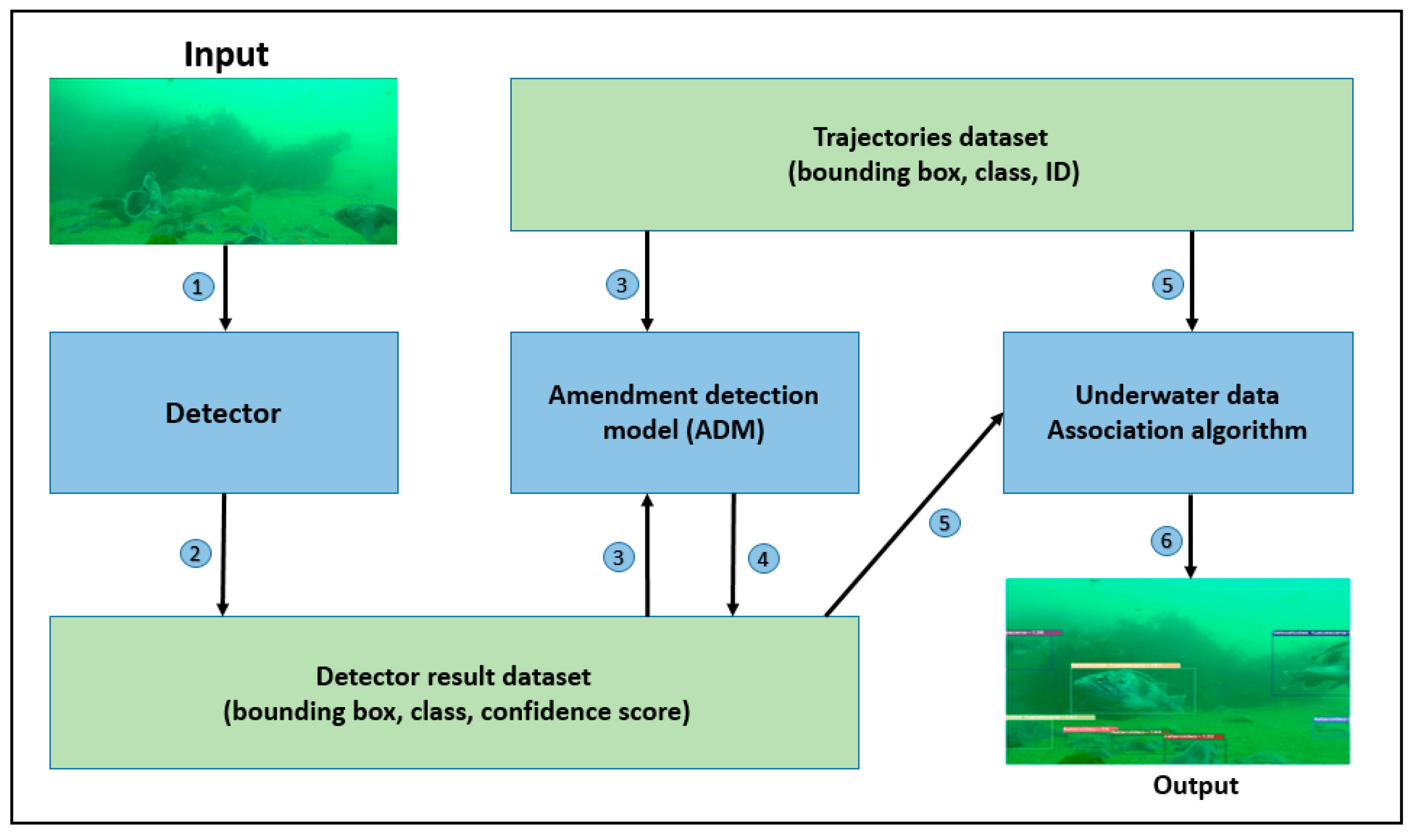
3. Method
The FSTA algorithm consists of an object detection module, an amendment detection model (ADM), and a data association module. The structure is shown in
Figure 1. The detector, such as the YoloX algorithm [
26], is used in the object detection module to obtain the objects’ classes, bounding boxes, and confidence scores from each frame. Then, the amendment detection model is used to improve underwater detection performance. Lastly, the detection results and current tracklets are inputted into the data association module to obtain trajectories.
3.1. Amendment Detection Model
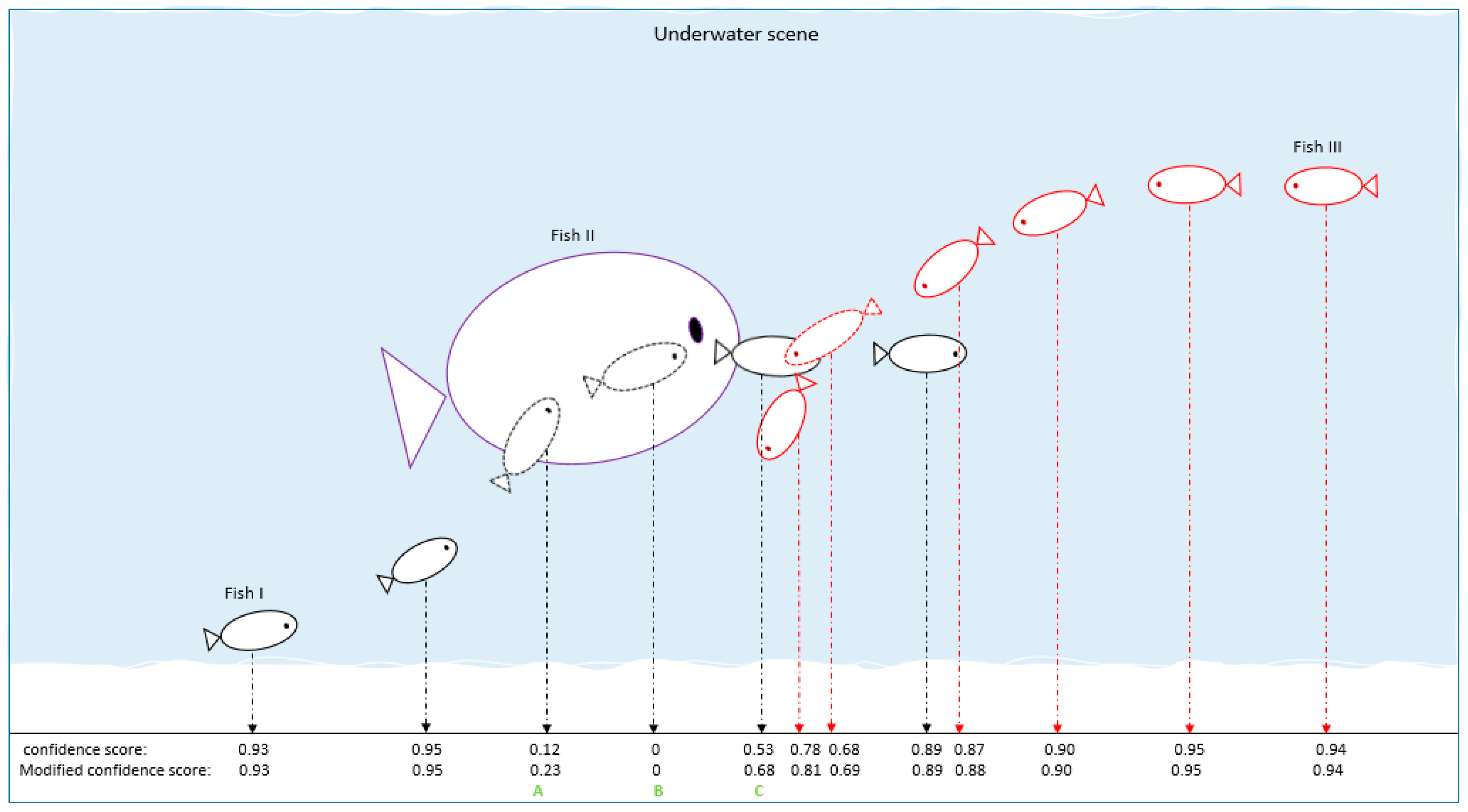
Underwater videos have problems of color distortion and blur, and fish features change over time. This can lead to inconsistent detection results. Therefore, we used tracklets to amend the detection results and improve the performance of the underwater detection model. The detection result seriously affects the result of the tracking algorithm on the basis of the tracking-by-detection paradigm. Here is an underwater scenario to illustrate the necessity of this module. In
Figure 2, black is Fish I, purple is Fish II, and red is Fish III. The first row at the bottom is the confidence score output by the detector model, and the second row is the modified confidence score. Fish II occluded Fish I at Point A, so Fish I was lost at Point A. When Fish I reappeared at Point C, it was partially occluded by Fish III, resulting in low confidence. Then, Fish I was not matched with the existing trajectory in the data-associated algorithm at Point C. Although the confidence score of the fish was low, we can infer that the reappeared fish was Fish I by observing the trajectory at Point C. The idea of this module is to use the current trajectories as prior knowledge. The fish’s confidence improves after the correction at Point C. The object can participate in the subsequent data association algorithm to improve the tracking performance.
The pseudocode of the ADM algorithm is shown below.
The input of ADM is a detection set
along with tracklet set
and Kalman Filter
. We also set a parameter
, which is an adjustable parameter related to the current image size and blur level. The output of ADM is the detection set
of the current frame containing the bounding box and class of the object. Tracklet set
is empty in the first frame. We merge tracked set
and currently lost set
into one set,
. Then, we use Kalman filter
to predict the new locations of each tracking bounding box. After that, we calculate the distances between each tracking box and each detection box usingIoU distance. (Lines 1 to 8 in Algorithm 1).
| Algorithm 1: Pseudocode of ADM |
| Input: detection set , tracklet set , adjustment parameter , Kalman filter . |
| Output: detection set |
| 1. Initialization: |
| 2. |
| 3. for in do |
| 4. |
| 5. end |
| 6. for in do |
| 7. |
| 8. end |
| 9. for in do |
| 10. |
| 11. /*(i.score means the confidence score of detected object i)*/ |
| 12. end |
| 13. Return |
Lastly, the softmax function normalized the distance between object i and all detection boxes. Then, we modify the object’s confidence score with IoU distance, and is an adjustable parameter related to the current image size and blur level. The output of ADM is the detection set of the current frame containing the bounding box and class of the object (Lines 9 to 13 in Algorithm 1).
3.2. Data Association Algorithm
We introduced the BYTE data association [
31] algorithm and improved the algorithm using the re-ID feature extractor network. Since fish are non-rigid organisms, and the motion model was complex, the Kalman filter was mainly modeled with a uniform motion model, so it was not reliable to predict the coordinate position of fish by only using position information. This tracks a false object when occlusion occurs in the video. Therefore, we combined the representation feature of the object and its location information. The tracking loss of the current data association algorithm was high, and we designed a new data association algorithm. The occlusion of the object changed over time; thus, the weights of the representation and location features were adjusted automatically to improve the performance.
The input of the data association algorithm is a video sequence along with an object detector and Kalman filter . We also set five thresholds: , , , , and . and are the detection score thresholds, is the tracking score threshold, is the match score threshold, and is the max lost frame number. The output of the data association algorithm is tracks of video sequence .
Each frame obtains the bounding boxes, confidence scores, and coordinates using the detector. All the detection boxes are divided into two parts,
and
, according to their detection score. The boxes whose scores are higher than
are classified as
, and the boxes whose scores are between
and
are classified as
(Lines 3 to 13 in Algorithm 2).
| Algorithm 2: Pseudocode of data association algorithm |
- Input:
video sequence , object detector, re-ID feature extractor , Kalman filter , detection score threshold , tracking score threshold , match score threshold , lost buffer frame number . - Output:
Tracks of the video.
|
| 1. Initialization: |
| 2. for frame in do |
| 3. |
| 4. |
| 5. |
| 6. for d in do |
| 7. if then |
| 8. |
| 9. end |
| 10. else if and then |
| 11. |
| 12. end |
| 13. end |
| 14. |
| 15. for in do |
| 16. |
| 17. end |
| 18. /*high score association*/ |
| 19. |
| 20. |
| 21. |
| 22. for m in do |
| 23. if then |
| 24. |
| 25. /*low score association*/ |
| 26. |
| 27. |
| 28. |
| 29. means the lost frame number of the object in the remaining track set)*/ |
| 30. Associate and |
| 31. |
| 32. /* delete unmatched tracks*/ |
| 33. |
| 34. for in |
| 35. if then |
| 36. |
| 37. end |
| 38. end |
| 39. end |
| 40. Return |
Tracked set and lost set are merged into one set, . Then, a Kalman filter () is used to predict the new coordinates of each track, as performed in ADM. We also use a re-ID network to obtain the representation feature of each object in track set (Lines 14 to 17 in Algorithm 2).
Next, we match detection bounding boxes
with the objects in track set
. The IoU is used to compute the similarity of all possible pairs, and we use a binary graph maximal matching algorithm, such as the Hungarian algorithm [
36], to accomplish their matching. Then, all the matched pairs are filtered by the Euclidean distance of their appearance feature, whose distance over
remains. Unlike tracking methods, only using predicted position information is easily affected by the distance of the boxes. This situation affects lost-target tracking and the matching false detection box on the track. The proposed method adds the apparent feature scores to discriminate between the different objects. At the end of this stage, only the unmatched detection objects in
and the unmatched track set objects in
remain (Lines 17 to 24 in Algorithm 2).
In the second stage of association, unmatched first-stage high-score detection set is added to low-score detection set . We associate objects between low detection set and remaining track set . We calculate the cost between and by the IoU distance and the re-ID feature distance. This cost change over lost time. The Hungarian algorithm is used to finish the matching on the basis of the cost (Lines 25 to 31 in Algorithm 2).
All remaining unmatched tracklets
after the second stage of the association are removed from tracked tracklets
if they are in
, and added into lost tracklets
. For simplicity, the procedure of tracking rebirth [
21,
30,
37] is not shown in Algorithm 2. Only if the target is not tracked for over 30 frames, i.e., the tracklet is added into
for over 30 frames, it is deleted from lost tracklet
, which means that the target left the camera forever (Lines 32 to 33 in Algorithm 2).
Lastly, the detection boxes that satisfy the following conditions are used to initialize new tracklets (Lines 33 to 39 in Algorithm 1). (1) They are from , which remains in the first association stage and is still not matched in the second association stage. (2) The detection scores are higher than , where . (3) The boxes are detected over two consecutive frames.
3.3. Re-ID Network
The performance of the re-ID network affects the results of the subsequent data-matching algorithm in multiple-target tracking experiments. So, it is necessary to obtain accurate feature extraction results from the re-ID network. The fish swim in all directions in the extraction process, and their characteristics vary a lot. In view of these facts, we adopte the heuristic dynamic feature fusion strategy and integrate the fish features extracted from multiple viewing angles to improve the feature representation ability of the network. A re-identification neural network is used to obtain the representation feature of the object. Thus, reducing the feature distances of the same object while enlarging the feature distances of different objects is a re-identification task. When occlusion and high turbidity occur, a common re-identification neural network has a poor effect and cannot enlarge the feature distance of different objects. Most research uses triplet loss to obtain more stable features. Furthermore, the triplet loss function is improved to achieve better performance. We improve the loss function by replacing instance-based loss with object-based loss. The feature of the object is gradually robust with the increase in the number of successfully matched frames, so the object could be rematched according to the local feature when occlusion occurrs.
Instead of using the triple loss function, the centroid triplet loss function is performed to train the re-identification network. The centroid triplet loss function is formulated in Equation (1), where [
z]+ =
max(
z, 0),
f denotes the re-identification network, and A is an anchor instance. Centroid triplet loss (CTL) computes the distance among an anchor instance, a positive class centroid
and a negative class centroid
.
The centroid is calculated as the mean feature of the same object in the video frames, as shown in
Figure 3. Thus, each object is represented by a single embedding along its lifetime, reducing retrieval time and storage requirements. The backbone of the re-ID network is Resnet50-IBN. Most CNNs use instance normalization (IN) or batch normalization alone. High-level visual tasks such as recognition use BN as a critical component to improve learning ability, while low-level visual tasks such as image style transformation use IN to remove the changing parts of pictures. IN eliminates the difference in individual appearance, but simultaneously reduces useful information. Resnet50-IBN reasonably combines IN and BN, which improves learning and generalization abilities.
4. Experiments and Results
To demonstrate the perfromance of the proposed fish tracking algorithm, we first elaborate on the dataset and implementation details in
Section 4.1. We compare the FSTA with other related methods and evaluate different settings to justify our design choices in
Section 4.2. Then, we show that our correlation tracker outperformed the state-of-the-art methods on five MOT benchmarks in
Section 4.3. Lastly, we visualize the tracking trajectories in
Section 4.4.
4.1. Dataset and Implementation Details
Dataset. Our neural network consist of the detection and re-identification networks. We used 5300 images as the training dataset of the detection network. The images were all extracted from the observation video of a marine pasture over one year. LabelImage software labelled the image according to the VOC format [
38]. Second, 6318 images were used as the training dataset of the re-identification network; the format of the dataset was similar to that of DeepFashion [
39]. The dataset is available at
https://drive.google.com/file/d/15BDaciElZRaAIZgDRFjl1iq_sVseDRqP/view?usp=sharing (accessed on 18 August 2022).
Implementation details. The training and reference of the algorithm were carried out on a server configured with Intel(R) Xeon(R) Gold 6342 CPU × two and NVIDIA A100 40 GB × 4 in this experiment. We used PyTorch to build the backbone network and ran it on the Ubuntu 18.04 LTS operating system.
We adopted YoloX as the detector and trained it on the input with a resolution of . We used random flip, random scaling (between 0.5 to 0.9), cropping, and data mosaic as data augmentation, and Adam to optimize the overall objective. The learning rate was initialized as and then decayed to in the last 20 epochs. We trained with a batch size of 32 (on 4 GPUS) for 120 epochs. When using the Adam optimizer, some networks may fall off a cliff and then fix at a value from which they are no longer able to recover. By reducing the learning rate to some threshold, such as 0.0001, unstable cases can be solved; the step size is then reduced to 0.000001 to ensure that the model gradually converges.
The backbone network of the re-identification network is Resnet50-IBN; the implementation and hyperparameters mostly follow Pan et al. and Wieczorek et al. [
40,
41]. The backbone network was pretrained on ImageNet, and then we fine-tuned the network in our dataset. We used
for the last convolutional layer and modified it to a 512-dimensional embedding size. The loss functions were similar to those in He et al. and Wieczorek et al. [
42,
43], and we used triplet loss, center loss, and classification loss. The center loss was weighted by a factor of
, and all other losses were assigned a weight of 1. The learning rate was initialized as
and then decayed to
in the last 25 epochs. The models were trained for 150 epochs because the loss function curve converged at the 150th epoch on the basis of our dataset. Note that, this value is related to the size of the dataset. Different datasets have different convergence speed levels. Usually, the larger the dataset is, the fewer the training epochs are needed.
In the data association algorithm, detection score threshold was set to 0.7, and was set to 0.2. The tracking score threshold was set to 0.6. The matching score threshold was set to 0.5. The maximal lost frame was set to 50.
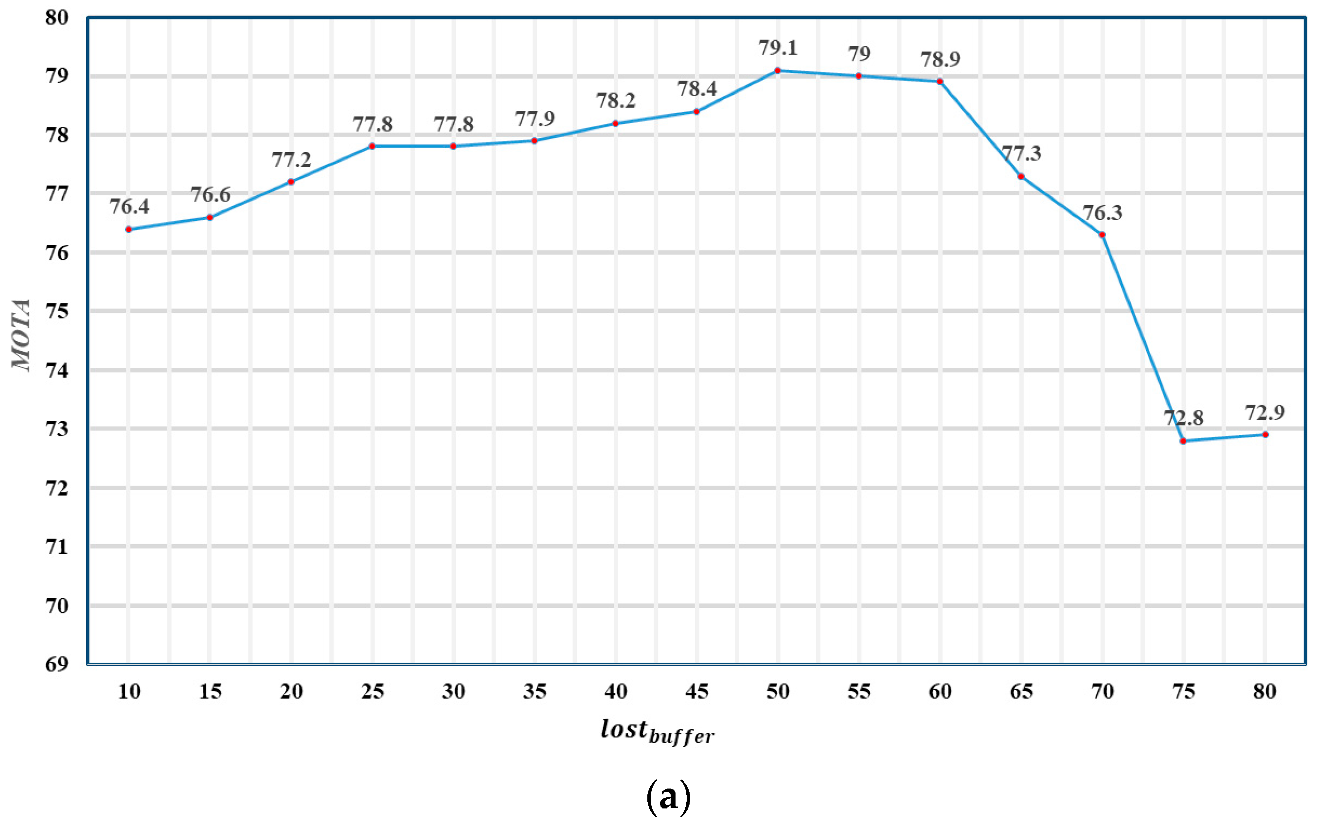
4.2. Hyperparameter Setting and Network Experimentaion
We first tested the hyperparameter setting. As
Figure 4a shows, when
< 50, MOTA does not decrease with the increase in
. When
= 50, the maximal MOTA reaches 79.1. Thus,
was set to 50 in this study. This value is related to the video’s frame rate and the fish’s swimming speed. The frame rate of the video that we tested is 30. If the frame rate of the video is not 30, additional adjustment of this hyperparameter would be needed. With a fixed
, we searched for the proper value of
. This value was used to control the matching accuracy; we only used the position prediction algorithm in the first association. When this value was too large, most successful matches were not filtered, so many wrong matches were considered to be correct, and the MOTA was significantly reduced.
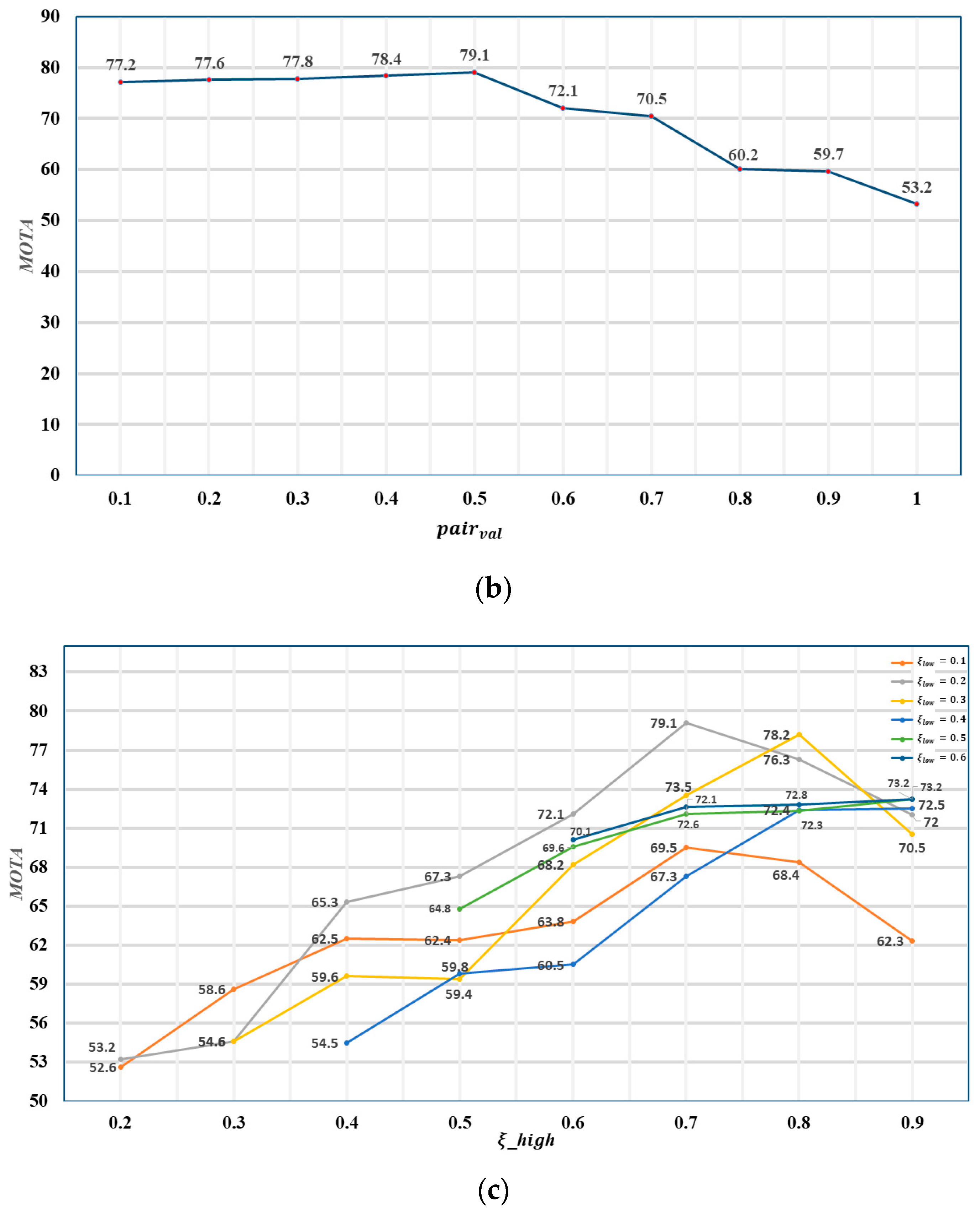
Figure 4b shows that, when
is 0.5, the result is the best.
and
controll the confidence score range of the two-stage data association algorithm and, to some extent, determine the reliability of the Kalman filter. In
Figure 4c, we present the tracking performance under different
and
. The result is better when the difference between the two values is around 0.5, among which
= 0.7 and
= 0.2 have the best result. When
, it becomes a one-stage data association algorithm using only position prediction.
Table 1 presents the achieved performance using different backbone models of reidentification networks. The top MOTA and the highest IDF1 are obtained with ResNet50-IBN. ResNet50-IBN means that we added IBN-Net into ResNet50. IBN-Net carefully integrated instance normalization (IN) and batch normalization (BN) as building blocks, and could be wrapped into ResNet50 networks to improve its performance without increasing computational cost. IN learns invariant features to appearance changes, such as colors, styles, and virtuality or reality, by delving into IN and BN. At the same time, BN is essential for preserving content-related information. This backbone is considered to run all the following experiments.
Table 2 shows the obtained performance by considering different input image resolutions. Better performance could be achieved with high image resolutions, but at a higher computational cost.
4.3. Ablation Study
We tested the effect of the above modules on the results, as shown in
Table 3. The baseline model was ResNet50 with a Kalman filter algorithm. Re-ID indicates that we add the representation feature into the data association algorithm in the baseline model. Then, the amendment detection model (ADM) is added into the baseline model. Centroid loss indicates the formula that is used as triplet loss. The baseline performs similarly to SORT, which has the best FPS, but we significantly improve the multiple-object tracking accuracy (MOTA), and the introduced representation features substantially reduce the ID switches.
4.4. State-of-the-Art Comparisons
We compared FSTA with other popular association methods: SORT [
29], DeepSORT [
30], JDE [
23] and ByteDance [
31]. The results are shown in
Table 4.
SORT can be considered as our baseline method because all methods only use a Kalman filter to predict the object’s motion. The FSTA improved the MOTA metric of SORT from 71.6% to 79.1% and IDF1 from 75.4% to 82.3%, and decreased the IDs from 342 to 160. This highlights the importance of the representation features, and proves the ability of FSTA to recover object boxes from a low-score one.
DeepSORT uses additional re-ID models to enhance long-range association. We surprisingly observed that the FSTA also had more significant gains than those of DeepSORT, which suggests that the cascade association is not the best algorithm, which could be improved by optimizing the data association structure and re-ID network.
JDE proposed a MOT system that allows for a shared model to learn target detection and appearance embedding. Specifically, it incorporates the appearance embedding model into a single-shot detector, such that the model could simultaneously output detections and the corresponding embeddings. The FSTA improves the MOTA metric of JDE from 76.1% to 79.1% and IDF1 from 72.2% to 82.3%, and decreases IDs from 453 to 160. It uses the idea of classification to fit the target ID, which causes the ID switch to be too large.
ByteDance suggests that a simple Kalman Filter can perform long-range association, and achieve better IDF1 and IDs when the detection boxes are accurate. However, it is difficult for the motion model to refine a lost object in severe occlusion cases. Therefore, representation features behave more reliably.
4.5. Visualization
The specific algorithm effect is shown in
Figure 5, in which frames of 10, 15, 40, 70, 100, and 130 s were intercepted from test video data. The mark in the figure is the scientific name and count of each category, respectively. This algorithm can be used as a long-term recognition algorithm for an underwater observation platform, and it not only meets the real-time requirements, but also has a high accuracy rate.
5. Discussion
By adding the robust Re-ID algorithm proposed in this study, the centroid-based matching algorithm improves its accuracy over time because more complete organism characteristics could be learned. We provide a visual comparison between our algorithm and another algorithm that only uses the location information in
Figure 6. There were three fish swimming in overlapping occlusion over time. We use a triangle to represent each fish, and the solid purple lines successfully represente the matched object. The dotted line is the unsuccessful match. Algorithm 1 is ours, and Algorithm 2 only uses the Kalman filter to predict the position of the coordinate to match the object. The fish swimming cover problem occurred in the 67th frame, and the algorithm lost the original target, but when Fish III reappeared in the 101st frame, Algorithm 1 could track the target. Algorithm 2 lost the target and gave it a new ID, which added tracking error.
This technology has its shortcomings. The motion model of Kalman filtering is a uniform motion model. When there is a large wave or fish mutation, the model affects the tracking result because fish are nonrigid. The problem can be solved through an improved motion model of the Kalman filter. Still, it is also difficult to build the fish motion model. We also tested the nonlinear particle filter with stronger overfitting ability, but its performance was not stable because it could only obtain local optimal solutions. If the global optimal solution could be obtained, the tracking performance could be effectively improved, and this could be a future breakthrough point.
Through experimental tests, the recognition accuracy rate dropped by 1.5% to 2.3% in other sea areas. This was due to different sea areas’ color cast and contrast differences. So, when the FSTA is applied to different sea areas, the network weight coefficients need to be retrained accordingly. By adding different white balance methods to process the video first, since the parameters of white balance need to be manually adjusted, the most appropriate method should introduce a color complement neural network before image classification. This would be another future breakthrough point.
This study is expected to have good prospects. First, our model was stably tested in marine ranches, and could achieve long-term and highly accurate underwater biological tracking. Second, our algorithm could be applied not only to underwater loading equipment, but also to underwater robots, underwater AUVs, and other equipment. The algorithm in this paper has the potential to realize automatic statistics in marine environments, and it can be a useful complement to traditional manual statistical methods. In addition, the algorithm provides a means to analyze underwater biological environments. By tracking the trajectory of fish, fish behavior can be analyzed; current water-quality and environmental changes can be further analyzed to provide an additional verification of observer data. The technology only needs to rely on high-definition underwater cameras without special requirements for the cameras, but there are certain restrictions on the observation and tracking time. For example, the time during which we could track was mainly during the day. Accuracy dropped at night and in particularly murky water, so there are specific light requirements.
6. Conclusions
Tracking methods based on deep learning rarely involve underwater-object tracking. Compared with processing in non-underwater photos or videos, underwater fish tracking is challenging due to varying marine environments and poor-quality underwater imaging. In this paper, we proposed a robust tracker FSTA, and its accuracy achieves 79.1% of MOTA and 82.3% of IDF1 on the basis of our underwater dataset.
The FSTA, as a new paradigm for underwater fish tracking, has the potential to be widely applied to aquatic observation systems. First, the image quality of underwater videos suffers from color distortions, deformations, low resolution, and contrast, and fish features vary over time. This also leads to inconsistent detection results because of the sudden low confidence scores during detection. Therefore, in this study, trajectories have been used as prior knowledge to amend the detection results to improve the performance of the underwater detection model. Second, a new data association algorithm is proposed by recombining representation and location information. In this algorithm, the weight parameters of the position and apparent information are dynamic. The loss value could be adjusted according to the lost situation to improve matching performance. We recovered objects from the low-score detection box while filtering out the background. The algorithm is robust to occlusion due to dynamic association, which improves retracing lost targets. Lastly, we introduce the centroid triplet loss function to train the RestNet50-IBN feature extraction network. This greatly enhances the performance of the tracking algorithm.
The different hyperparameters affect our algorithm’s performance. The effects of the three components of the algorithm in this paper have been tested with ablation experiments. The experimental results show that each element improved the model’s performance in a different aspect, and among them, the Re-ID network showed superior performance. Also, the results of our model were compared with the performance of state-of-the-art algorithms, and our algorithm has indices in the leading position for the underwater dataset. In addition, the shortcomings of the model has also been discussed in this paper, and further improvement could be achieved by focusing on the unresolved complex fish aliasing phenomena.


