Article

Quantifying Spatiotemporal Heterogeneities in PM2.5-Related Health and Associated Determinants Using Geospatial Big Data: A Case Study in Beijing

1
College of Applied Arts and Sciences, Beijing Union University, Beijing 100191, China
2
Laboratory of Urban Cultural Sensing & Computing, Beijing Union University, Beijing 100191, China
3
International Research Center of Big Data for Sustainable Development Goals, Beijing 100094, China
4
Key Laboratory of Digital Earth Science, Aerospace Information Research Institute, Chinese Academy of Sciences, Beijing 100094, China
5
State Key Laboratory of Remote Sensing Science, Aerospace Information Research Institute, Chinese Academy of Sciences, Beijing 100094, China
6
College of Resource Environment and Tourism, Capital Normal University, Beijing 100048, China
*
Author to whom correspondence should be addressed.
Remote Sens. 2022, 14(16), 4012; https://doi.org/10.3390/rs14164012
Submission received: 27 July 2022 / Revised: 13 August 2022 / Accepted: 16 August 2022 / Published: 18 August 2022

Abstract

:
Air pollution has brought about serious challenges to public health. With the limitations of available data, previous studies overlooked spatiotemporal heterogeneities in PM2.5-related health (PM2.5-RH) and multiple associated factors at the subdistrict scale. In this research, social media Weibo data was employed to extract PM2.5-RH based on the Bidirectional Encoder Representations from Transformers (BERT) model, in Beijing, China. Then, the relationship between PM2.5-RH and eight associated factors was qualified based on multi-source geospatial big data using Geographically Weighted Regression (GWR) models. The results indicate that the PM2.5-RH in the study area showed a spatial pattern of agglomeration to the city center and seasonal variation in the spatially non-stationary effects. The impacts of varied factors on PM2.5-RH were also spatiotemporally heterogeneous. Specifically, nighttime light (NTL), population density (PD) and the normalized difference built-up index (NDBI) had outstanding effects on PM2.5-RH in the four seasons, but with spatial disparities. The impact of the normalized difference vegetation index (NDVI) on PM2.5-RH was significant in summer, especially in the central urban areas, while in winter, the contribution of the air quality index (AQI) was increased. This research further demonstrates the feasibility of using social media data to indicate the effect of air pollution on public health and provides new insights into the seasonal impacts of associated driving factors on the health effects of air pollution.

Graphical Abstract

1. Introduction

Air pollution is a major global public health issue [1], which is ranked as the fifth greatest risk factor for global mortality in the Global Burden of Disease (GBD) [2]. Exposure to air pollution can cause diseases such as stroke, lung cancer, and mental disorders, which can lead to death in extreme cases [3,4,5]. China has faced serious air pollution problems due to rapid urbanization [6]. Although China has conducted a series of clean air initiatives, the health costs and risks caused by air pollution remain high [7]. In 2020, there were 997,955 premature deaths related to particulate matter 2.5 (PM2.5) in China [8]. The health cost of air pollution in Beijing in 2020 was approximately RMB 6505.84 million, accounting for 0.17% of its GDP [9]. Therefore, the issues of PM2.5-related health (PM2.5-RH) should continuously concern scholars and government decision makers.
In recent years, research on the spatiotemporal heterogeneities in air pollution-related health has been carried out extensively at varying spatial scales. On the regional macro-scale, Chen et al. explored the spatial-temporal variation of exposure to PM2.5 in Chinese around the world [10]. Ji et al. explored the spatial heterogeneity of the sensitivities to air pollution in 70 Chinese cities [11]. In addition, regional and seasonal variations in exposure to PM2.5 were systematically analyzed [12,13]. A growing number of studies have concentrated on Chinese urban agglomerations in recent years, especially in those regions with serious environmental problems, such as the Beijing–Tianjin–Hebei region [14], the Yangtze River Delta [15], and Central China [16]. These studies have strongly demonstrated the spatiotemporal heterogeneities of the impact of air pollution on health at the regional scale. On the other hand, the spatiotemporal variations in air pollution-related health were associated with extensive and complex factors due to the differences in economic activities and the natural environments [17]. It has been documented that nighttime light (NTL) [18] and GDP [19] were negatively correlated with exposure to air pollution. Chen et al. put forward that high population density worsens the local air quality [20]. There were also obvious differences in the impact of the natural environment [21]. For instance, exposure to air pollution along with high temperatures was likely to increase the odds of respiratory mortality [22]. As one indicator of vegetation density, the normalized difference vegetation index (NDVI) was obviously correlated with air quality, as well as improved health, due to the functions of vegetation as absorbers and barriers to air pollutants [23,24]. There were also reports documented that the public perception of air pollution might be inconsistent with objective air quality, which was evaluated using scientific indices such as the air quality index (AQI) [25]. Although there were regional differences in the intensity and direction, the influences of the built environment on PM2.5-RH, such as parks, greenways, and urban form, have been widely studied [26,27,28,29,30]. For instance, buildings create obstacles and disturbances to the wind, which thus affect the air quality in urban areas [31]. Road density, defined as the ratio of road surface area to city territory size, was negatively correlated with particulate matter 10 (PM10) [32], the same as the result of the land use mix [33]. Furthermore, additional improvements in air quality should take seasonality into account, because factors may play different roles in different seasons [34,35]. These studies showed that PM2.5-RH was impacted by multiple factors. However, with the limitation of the currently available data, previous studies were mostly focused on either a single factor or on large-scale regions. There were research gaps by ignoring combining multiple factors or spatial heterogeneities at the fine scale. Further research is necessary to make clear spatiotemporal heterogeneities of multifactorial effects of PM2.5-RH at the fine scale within inner cities, which is conducive to providing targeted advice in urban planning [36].
Moreover, from the perspective of the data used in previous studies, statistical or survey data were commonly employed, such as outpatient number, number of cases, mortality, and health care costs [37,38]. However, it was difficult to access to above data, and there were also limitations with the timeliness [39]. Furthermore, the health of susceptible and sensitive individuals can be impacted even on low air pollution days [40]. Most of the above indicators were targeted at already manifested diseases at the top of the health impact pyramid [41], which may lead to ignoring those people who were in a sub-healthy state or felt uncomfortable due to air pollution. Therefore, such statistical or survey data cannot comprehensively reflect PM2.5-RH [11]. With the advantage of being easy to access, timely, and rich in semantic information, social media data have powerful potential for perceiving the health status of residents [42]. Twitter data have been used to aid in public health efforts concerned with surveillance, event detection, pharmacovigilance, forecasting, disease tracking, and geographic identification, demonstrating positive results [43]. It was also found that health status reflected by social media data was highly correlated with the actual number of cases [44]. As the most widely used social media platform in China, Weibo has been widely applied to measure well-being, sensitivity, and health effects related to heat waves, air pollution, and epidemics [11,45,46,47]. Moreover, the Weibo platform supports users to share geolocation information anytime and anywhere. Although the spatial positioning of Weibo is uncertain [48], relevant studies have demonstrated its ability to portray intra-city differentiation patterns when combined with traditional spatial data [49]. It was widely used in population spatiotemporal behavior and natural disaster management [49,50]. Thus, it provided an effective data source to explore the PM2.5-related health within the city [51].
Therefore, our research intended to explore the spatiotemporal heterogeneities in PM2.5-RH at the subdistrict scale and quantify the impact of the multiple associated factors based on Weibo data and other multisource geospatial big data, taking Beijing, China, as the study area. Specifically, this research had the following two objectives: (1) to mine the real-time expressed health information related to PM2.5 in Beijing based on Weibo data; (2) to explore spatiotemporal heterogeneities of factors associated with PM2.5-RH using GWR models. The paper is organized as follows. Section 2 introduces the study area, the materials, and the methods. Then, the results and comprehensive descriptions are presented in Section 3. Section 4 discusses the findings of this paper in detail. Finally, Section 5 concludes the research by summarizing the findings.

2. Materials and Methods
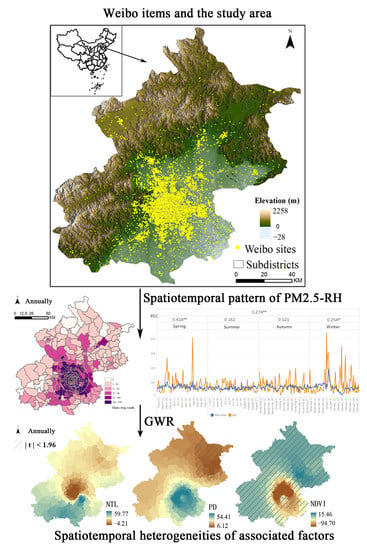
2.1. Study Area

Beijing is the center of politics in China, with a long history of civilization and cultural integration. It covers an area of 16,410.54 km2, with plains accounting for 38.6% and mountains for 61.4% [52]. The total population of Beijing was 21,886,000 at the end of 2021. With rapid economic development, air pollution has become an increasingly serious problem in Beijing. It was estimated that the average concentration of Beijing’s PM2.5 in 2017 (116 μg/m3) was much higher than the WHO-recommended standard (10 μg/m3) [53]. The poor air quality had serious effects on residents’ health. This research highlighted the spatial variations in PM2.5-related health at the subdistrict scale. According to the National Earth System Science Data Center (http://www.geodata.cn, accessed on 20 November 2021), there are 328 subdistricts in Beijing, which are shown in Figure 1.

2.2. Dataset and Methods

2.2.1. Extracting PM2.5-RH Based on Weibo Data

As one of the largest and most influential blogging sites in China [54], the Sina Weibo platform has a predominantly young, educated, and engaged public audience [55]. Up to 30 September 2017, the number of monthly active users on Weibo increased to 376 million (https://socialone.com.cn/weibo-user-trends-report-2017/, accessed on 4 April 2022). Although these digital reflections of reality could be biased and partial due to the differences in user age, occupation, and geographic location [56], Weibo data continues to be one of the most useful data sources in public health [51]. In this research, 11.79 million Weibo items in Beijing in 2017 were obtained from the Weibo social media platform using web crawler technology. Each Weibo item includes the ID, textual content, time, latitude, and longitude. The PM2.5-RH was extracted based on the Weibo data following the procedures listed below.
Firstly, those Weibo items about PM2.5-related health (PM2.5-RH) were extracted based on the textual content in the Weibo data using the Bidirectional Encoder Representations from Transformers (BERT) model [57]. As an unsupervised Transformer learning method proposed by Google, BERT is a model trained with a large number of unlabeled texts that can learn grammatical structures and analyze contextual relationships. For this purpose, all the Weibo items were firstly filtered by such key words as ‘haze’, ‘cough’, ‘headache’, and ‘breathing’. Then, a sample set of 10,000 items was selected randomly. Each item was marked manually as 1 if the text content is related to PM2.5-RH, otherwise 0. For example, people commented on the Sina Weibo platform about feeling discomfort due to air pollution, with examples such as ‘The smog is killing my throat’ and ‘The heavy pollution outside makes my lungs ache’. The labeled sample sets were divided into a training set (80%) and a verification set (20%), which were input into the BERT model for training and accuracy verification. A classifier with high accuracy was selected to input all Weibo items into the training model for classification. By adjusting the learning rate and the number of iterations, the overall accuracy of the BERT classifier was over 86%. A total of 21,372 Weibo items were finally extracted by the BERT model.
Secondly, the numbers of above-derived Weibo items for each subdistrict were calculated to indicate the PM2.5-related health at the subdistrict scale. Here, the Weibo sites were geocoded by the latitude and longitude in the Weibo data. Then, it was overlaid with the subdistricts to conduct the regional statistics. Moreover, as the sample of Weibo user groups was biased according to the Weibo User Trends Report in 2017 (https://data.weibo.com/report/, accessed on 4 April 2022), the population proportion (15–59 years old) was used to correct the number of extracted Weibo items. Based on the cellular signaling data provided by Smartsteps (www.smartsteps.com, accessed on 15 November 2021), the proportion of people aged 15–59 was calculated respectively in each subdistrict. Then, the PM2.5-RH was indicated by correcting the extracted Weibo items based on the following formula.
y i = x i / r i
where i is the name of subdistrict in Beijing; y represents PM2.5-related health; x indicates the number of Weibo items about PM2.5-RH; r denotes the proportion of the population aged 15–59 in each subdistrict.
Finally, to explore temporal variations, this research divided the year into spring (March–May), summer (June–August), autumn (September–November), and winter (December–February), according to meteorology. All the PM2.5-RHs based on the Weibo items were grouped into four categories by season based on the time in the Weibo data.

2.2.2. Deriving Associated Factors Based on Multi-Source Data

As mentioned above, multiple factors comprehensively affected the variations in PM2.5-RH. By reviewing previous research [18,19,20,21,22,23,24,25,26,27,28,29,30,31,32,33], we selected eight associated factors to explore the spatiotemporally heterogeneous in the determinate factors, including road network density, land use mix, the Normalized Difference Built-up Index (NDBI), the Air Quality Index (AQI), temperature, the Normalized Difference Built-up Index (NDVI), nighttime light (NTL), and population density. All the original data were processed and overlayed with the subdistricts in Beijing to obtain the variable values of each subdistrict in different seasons. The detailed information of the data used in this research is summarized in Table 1. The specific processing procedures are explained as follows.
NDBI, NDVI, temperature, and NTL were obtained from the satellite remote sensing data. They were extracted through Google Earth Engine (https://earthengine.google.com/, accessed on 10 November 2021), a platform powered by Google Cloud Computing that provides global-scale geospatial information data-processing services [58]. It allows for fast and parallel processing of large amounts of data resources, regardless of time and geographical constraints. We calculated different factors by three products of MODIS data and VIIRS_DNB data, which were extracted from GEE. Nighttime light data were provided by the Earth Observation Group (https://eogdata.mines.edu/products/vnl/, accessed on 10 November 2021), which were monthly nighttime day/night band composite products at a spatial resolution of 500 m. The other three MODIS products were provided by NASA LP DAAC at the USGS EROS Center (https://lpdaac.usgs.gov/products/, accessed on 10 November 2021). Specifically, NDVI data were obtained from the MOD13Q1 products. It had a spatial resolution of 250 m and a temporal resolution of a 16-day interval. NDBI data were calculated based on the MOD09A1 products at a spatial resolution of 500 m and a temporal resolution of an 8-day interval. The product contained matched-band 1-to-7 data acquired by the MODIS sensor, using reflectance values from band 2 (0.841 μm to 0.876 μm) and band 6 (1.628 μm to 1.652 μm) to calculate NDBI. Daily land surface temperature products (MYD11A1) had a spatial resolution of 1 km. After all remote sensing data were preprocessed (re-project, clip, and reclassify) using ArcGIS 10.6, all the variables were seasonally averaged and overlaid with the administrative boundary of each subdistrict variable. Finally, the quarterly values of four associated factors (temperature, NDVI, NDBI, and nighttime light) for each subdistrict were obtained.
It has been demonstrated that point of interest (POI) accurately reflects the current land use characteristics at a fine-grained level [59]. Based on the open API interface of Amap, a total of 1,369,572 POI data in Beijing in 2017 were crawled. The data included 23 categories, including: food and beverage services, scenic beauty, public facilities, business housing, and shopping services. In this research, the Gini Simpson Concentration Index (q = 2) of the Hill Numbers Biodiversity Index [60] was selected to measure the mixed distribution of land in Beijing [61].
D = 1 / ( i = 1 n P i 2 )
where D represents diversity, n represents the number of POI species, and P indicates the relative diversity, which can be area ratio or quantity ratio, etc. Parameter 2 was a rank, which reflected the sensitivity of the diversity index to the species.
The air quality index (AQI) presented six pollutants (PM10, PM2.5, SO2, NO2, CO, O3) on a single rating scale that described the degree to which the air was clean or polluted [62]. The data were obtained from the online platform monitoring and analyzing air quality. As the distribution of air quality-monitoring stations was scattered, the AQI was discontinuous in the study area. Therefore, following the method of calculating air pollution products on Geospatial Data Cloud (http://www.gscloud.cn, accessed on 2 November 2021), we selected the Kriging interpolation method to produce the continuous data [63]. After calculating the quarterly AQI of 12 air pollutant-monitoring stations, the spatial distribution of AQI in Beijing was simulated by ordinary kriging interpolation. Finally, the quarterly AQI of each subdistrict was obtained.
The road network data were obtained from OpenStreetMap (https://www.openstreetmap.org/, accessed on 20 November 2021), with corresponding data cleaning and deduplication. The method was to calculate the ratio of road length to the subdistrict area by superimposing road network data and Beijing subdistricts. The population density data in 2017 in Beijing were derived from the World Population Dataset (https://www.worldpop.org/, accessed on 20 November 2021). Each grid (30 arc seconds, approximately 1 km) represented the total number of people (unit: person/km2) within the area. It was obtained after processing, such as a merger, transformation, and clipping.
In addition, all the administrative boundaries on the scale of 1:4,000,000 maps were obtained from the National Earth System Science Data Center (http://www.geodata.cn/, accessed on 2 November 2021). These boundaries were used to separate subdistricts for the study area.

2.2.3. Geographically Weighted Regression Model

In this research, the spatial non-stationary relationship between PM2.5-RH and associated factors were quantified using the Geographically Weighted Regression (GWR) model. The GWR model was proposed by Fotheringham et al., which extended the traditional regression model (e.g., OLS) by adding regional parameters [64]. It obtained local parameters rather than global ones, the former being functions of position and therefore varying with space. The GWR model can be expressed as:
y i = β 0 ( μ i , v i ) + k = 1 p β k ( μ i , v i ) x i k + ε i
where ( μ i , v i ) represents the coordinate location of the ith point, and k expresses the independent variable number. y i , x i k , ε i , respectively, denote the dependent variable, the independent variables, and the random error term at location i. β 0 ( μ i , v i ) is the intercept for location i, and β k ( μ i , v i ) is the slope coefficient for x k at location i. The parameters were estimated from:
β ( μ i , v i ) = ( X T W ( μ i , v i ) X ) 1 X T W ( μ i , v i ) Y
where β ( μ i , v i ) represents the unbiased estimate of the regression coefficient. W ( μ i , v i ) is the weighting matrix which acts to ensure that observation near to the specific point have a bigger weight value, and X and Y are matrices for independent and dependent variables. The weighting function, called the kernel function, can be stated using the exponential distance decay from:
ω i j = exp ( d i j 2 b 2 )
where ω i j represents the weight of observation j for location i, dij expresses the Euclidean distance between points i and j, and b is the kernel bandwidth. If observation j coincides with i, the weight value is one. If the distance is greater than the kernel bandwidth, the weight is set to zero.
When conducting GWR models in this research, the covariance method was used to test the collinearities between variables. The F-test was used to determine the existence of spatial non-stationarity in the variables’ association with PM2.5-RH. The adjusted R-square was used to indicate the goodness of fit of the models. In addition, the t-test was used to judge the significance of local regression coefficients. Figure 2 shows the research framework in this research.

3. Results

3.1. Spatiotemporal Variations in PM2.5-RH

Figure 3 shows the comparison between the observed AQI (yellow curve) and the numbers of Weibo items about PM2.5-RH based on the BERT model (blue curve) in Beijing. The study lasted from 1 January to 31 December, 2017, and was also divided into the four seasons. AQI and PM2.5-RH shared the Y-axis. The Pearson correlation coefficients (PCC) between PM2.5-RH and AQI were analyzed for each season and annually. It was used to explore the relationship between the observed AQI and our extracted Weibo items about PM2.5-RH, and further corroborated the reasonableness of our methodologies. It can be seen that the correlation coefficient between annual AQI and PM2.5-RH was 0.274, which is statistically significant at the 0.01 level. According to the correlation coefficients in the four seasons, PM2.5-RH and AQI were significantly positively correlated in spring and winter, with a small correlation in summer and autumn. The highest correlation coefficient was found in spring, with a PCC value of 0.418. In general, the extracted PM2.5-RH based on the Weibo data using the BERT model could be used to indicate PM2.5-related health.
Figure 4 shows the spatial variations in PM2.5-RH in the four seasons and annually. It can be seen that the number of Weibo items about PM2.5-RH in Beijing varied greatly across different seasons and subdistricts. The global Moran’s I of PM2.5-RH in spring, summer, autumn, and winter were 0.52, 0.58, 0.48, and 0.50 (p-value < 0.001), respectively, and that for the annual was 0.54 (p-value < 0.001), which indicates the significant spatial autocorrelations in the spatial pattern of for PM2.5-RH. Namely, there were significant agglomeration characters. The number of Weibo items about PM2.5-RH in urban areas was more serious than that in suburban areas. Here, we used the average value as the measuring index to select those subdistricts with more Weibo items about PM2.5-RH. Taking the annual result as an example (Figure 4 and Figure 5), the number of Weibo items about PM2.5-RH was above 72 (the average value in the study area) in 35% of subdistricts, with the highest PM2.5-RH (>100) accounted for in 26.9% of all the subdistricts. They were mainly distributed within the Sixth Ring Road, especially on College Road in Haidian District, which was as high as 470. Those subdistricts with the lowest level (<5) were primarily located in the outer suburbs of Beijing, such as Huairou, Pinggu, Miyun, and Yanqing Districts, along with a few subdistricts in Fangshan District. The results reveal that there were significant spatial disparities in PM2.5-RH between various subdistricts in Beijing.
The seasonal variations of PM2.5-RH can be compared in Figure 4a–d. In general, the number of Weibo items about PM2.5-RH decreased in summer. The distribution of PM2.5-RH in spring and autumn was similar. Specifically, the highest PM2.5-RH in spring, summer, and autumn all occurred on College Road, with a high of 145 in spring and a low of 93 in summer. Within the Sixth Ring Road, PM2.5-RH in southern subdistricts increased in winter, while it was higher in northern subdistricts in spring and autumn. The highest PM2.5-RH in winter was 115, which occurred on DongHuaMen Road. In winter, PM2.5-RH was lower in subdistricts in outer suburban areas such as Huairou District and inner suburban areas such as Mentougou District.

3.2. Performances of the GWR Models

In this research, the GWR models were employed to explore the relationship between the associated factors and PM2.5-RH, which were completed in GWmodelS. We constructed five models with the dependent variable (PM2.5-RH) and eight independent variables in the four seasons and annually, respectively, namely: road network density, land use mix, NDBI, AQI, temperature, NDVI, NTL, and population density. Figure 5 shows the spatial distribution of eight associated factors annually at the subdistrict level (only annual values were shown due to the limitation of space).
To eliminate the influence of different units when conducting the models, all the variables were standardized. In addition, collinearity tests for the eight explanatory variables were completed using SPSS 19.0. The VIF values of the eight explanatory variables were all less than 10 in the four seasons and annually, indicating that there was no collinearity between variables. We used the AIC criterion method to determine the optimal bandwidth and construct the spatial weights as a Gaussian function. The results show that all five models passed the F-test at a significance level of 0.01, indicating that the models as a whole were spatially non-stationary. The adjusted R-square for all five models exceeded 0.5 (Table 2), with a good overall fit.

3.3. Spatiotemporal Heterogeneities in the Associated Determinates

The five statistical values of minimum, maximum, median, mean, and standard deviation of the regression coefficients for each factor were calculated and are summarized in Table 3. It can be seen that the regression coefficients of the eight correlated factors vary considerably, which intuitively reveals that they have distinct impacts on PM2.5-RH in different seasons. For example, in spring, the temperature had a positive effect on the global PM2.5-RH (mean 2.53), while NDVI showed an overall inhibitory effect (mean −7.27), and the effect was relatively greater. Specifically, the four associated factors of land use mix, NTL, population density, and road network density showed positive effects in the study area, while other factors showed different seasonal disparities.
The regression coefficients and the t-test value of each indicator for each subdistrict were visualized to explore the spatiotemporal variations, which are shown in Figure 6. The unlined regions in Figure 6 represent those regions where the t-values were between −1.96 and 1.96, indicating a statistical insignificance. With the limitation of space, we have selected the top three factors with large impact coefficients for each season to show the spatial distributions. For example, the inhibitory effects of NDVI on PM2.5-RH increased significantly in summer, especially in the central urban areas. In winter, AQI increased the effects on PM2.5-RH. NTL, population density, and NDBI had greater effects on PM2.5-RH in all four seasons, but with spatial disparities. The spatiotemporal heterogeneities of each factor on PM2.5-RH were analyzed separately in the following.
The two most significant factors contributing to PM2.5-RH were population density and NTL, with t-tests of their regression coefficients both passing at over 70%. The spatial patterns were also similar, with a high south and low north, with the central city larger than the suburbs. Seasonally, the peak area of population density influence gradually moved southward from urban areas. In addition, the effects of population density on PM2.5-RH differed seasonally, being stronger in autumn and slightly weaker in summer. The impacts of NTL on PM2.5-RH in Fangshan and Daxing districts were stronger in spring and summer but increased in Chaoyang district in autumn and winter. Overall, the impacts were much higher in winter (11.92) than in other seasons. NDVI showed a very significant negative effect on PM2.5-RH in subdistricts close to urban areas, while there was a positive trend in suburban Beijing. Among them, a significant negative correlation trend mainly existed in the subdistricts of Chaoyang and Haidian Districts. From a temporal perspective, the suppressive effect of NDVI on PM2.5-RH was more pronounced in summer (−13.72) and weaker in winter (−0.59). The negative correlation effects of NDBI on PM2.5-RH were similar to the spatial pattern of NDVI. Seasonally, there were significant suppressive effects on PM2.5-RH in central and south-western Beijing, especially in spring. AQI had both positive and negative location-specific spatiotemporal effects on PM2.5-RH in Beijing. Among them, a positive correlation trend mainly existed in the northern part of Beijing, such as Miyun, Huairou and Yanqing Districts. However, there was a significant negative correlation trend between AQI and PM2.5-RH variation in the south-western districts of Changping, Mentougou, and Fangshan. In the central areas, the correlations were negative in spring and winter, but the opposite in summer and autumn. The higher the temperature, the more serious PM2.5-RH in most parts of Beijing. In addition, in urban areas, especially Haidian District and Chaoyang District, there were obvious positive effects. Road network density significantly promoted PM2.5-RH in northwest Beijing. In terms of season, autumn had the greatest influence (4.32), which was distributed in Haidian District. Land use mix significantly promoted PM2.5-RH in the southern part of Beijing, especially in Daxing District, but had weak effects in the northern part.

4. Discussion

4.1. Analysis on PM2.5-RH Based on Weibo Data

With an increasing number of people posting publicly to express their experiences and attitudes toward air pollution, social media data can be a valuable resource to support ambient air pollution monitoring [65]. Not only can its textual content be used to extract information related to public health, but location can also support the extraction of intra-city-scale data. They were also time-sensitive and broad. Although many efforts had been made to extract the public health based on Weibo data [45,46,47,51], most of them overlooked that social media data suffers from sampling bias [66]. In this research, we tried to correct the errors by the proportion of the young population in the subdistricts and then explore the spatiotemporal variations in PM2.5-RH at the subdistrict scale.
PM2.5-RH showed an obvious spatial pattern of agglomeration to the city center. The high values were mainly distributed in subdistricts within the Sixth Ring Road and less so in the outer suburbs of Beijing. The urban area of Beijing was more densely populated, with 78% of the population located within the Sixth Ring Road. This indicated that urban residents were more sensitive to air pollution and more adversely affected [67]. It was also due to the concentrated distribution of the population, which would lead to more people posting microblogs in urban areas. In addition, PM2.5-RH showed different seasonal variation patterns. The distribution of PM2.5-RH was more correlated with the actual AQI in spring, and the fluctuation range of PM2.5-RH was larger in winter. The general fluctuation of PM2.5-RH was much less in the summer, with the seasonal PM2.5-RH minimums occurring in summer for most subdistricts. This indicated that residents were less sensitive to air pollution in summer, especially in central urban areas. In summer, the air was more mobile and pollutants are harder to collect [68], so the total weibo items about PM2.5-RH were lower. In a previous study, air quality tended to be more severe in winter because of coal burning [14]. The results of our research show that the total amount of PM2.5-RH was less in winter than in spring. This may be due to frequent dust storms in northern China that occur mostly in spring, when PM frequently reached peak levels [34]. Moreover, it indicated that there was a difference between the actual air pollutant concentration and residents’ perception of air pollution. According to the 2017 Beijing Municipal Environmental Status Bulletin, Beijing experienced continuous heavy pollution from March to April. Especially in late April, the air pollution alert level has been escalating. Continuous exposure to air pollution increased residents’ negative responses to air pollution on the Sina Weibo platform.

4.2. Relative Importance of the Associated Factors

Based on the GWR models, it was possible to compare the effects of various factors across different subdistricts and in different seasons. The effects of the eight related factors on PM2.5-RH in this study were spatially different at the subdistrict scale, as well as heterogeneous in the seasons.
Those subdistricts that are densely populated and have high NTL were much affected by air pollution. This was closely related to regional economic development. The finding is in line with previous observations that higher population density worsens local air quality due to human activities [20,69]. In this research, NTL had a high t-test pass rate, indicating that its impact cannot be ignored. However, it was insignificant in most central urban areas, which means that the relationships between PM2.5-RH and economic development are rather complex. More in-depth subsequent research is deserved in the future. We can still conclude that PM2.5-RH was higher in subdistricts with higher NTL. Our results show that low PM2.5-RH was found in subdistricts with high NDBI in all four seasons. the building density tended to have an adverse effect on air quality because of windless zones that are not beneficial for pollutant dispersion [70]. However, building density and building height have relatively limited and inconsistent effects in most cities [29]. It was documented that building density was negatively associated with PM2.5-RH [30]. This may be due to the limitations of the complicated mechanisms of pollutant dispersion and ventilation in realistic 3D urban environments.
NDVI had obvious temporal heterogeneity in relation to PM2.5-RH, with the effect stronger in summer. The influence was more significant within the Sixth Ring Road. As vegetation has the potential to mitigate air pollution [23,24], higher vegetation coverage could reduce residents’ discomfort with air pollution. In central urban areas, green space has a more significant positive impact on improving public health [71]. In the densely forested western region, due to low population density, the influence was relatively small. It is worth noting that the influence of AQI increased significantly in winter, while the influence of NDVI decreased significantly compared with other seasons. In addition to the reduction in vegetation during winter, the AQI impact rose due to a large amount of coal burned as a result of heating. Heating causes AQI to increase 1.4 times compared to the seasonal average [72]. Interestingly, there was significant spatial heterogeneity in the influence of AQI, with a positive effect in the northeast of Beijing and an opposite effect in the south. This may be due to the spatial distribution of air pollution showing a high southern and low northern profile [73].
In addition, the results for temperature, road network density, and land use mix were relatively less influential. The higher the temperature, the more serious PM2.5-RH in most subdistricts of Beijing. This is consistent with the findings of prior studies, which showed that temperature is positively associated with PM2.5-RH. On social media platforms, higher temperatures also led to more negative health ratings from residents. Land use mix was shown to contribute to the PM2.5-RH overall in different seasons. A high percentage of mixed land uses could also indicate a relatively high density of restaurants, shops, and manufacturing facilities that may act as local pollution hotspots [30].

5. Conclusions

Based on the social media Weibo data, the spatiotemporal variations in PM2.5-RH in Beijing was mapped in this research. The GWR models were then employed to explore the relationship between associated factors and PM2.5-RH in Beijing. This study further demonstrated the feasibility of using social media data to study PM2.5-RH. In addition, this research provided important insights into the seasonal impact of associated determinate factors on PM2.5-RH. Importantly, eight associated factors discussed in this research showed he seasonal variation in the spatially non-stationary effects.
Specifically, there were obvious spatiotemporal variations in PM2.5-RH in Beijing. PM2.5-RH showed a spatial pattern of being greater in the Sixth Ring Road than in the suburbs. There were also seasonal disparities in PM2.5-RH in different subdistricts. In terms of the associated determinants, there were obvious spatiotemporal heterogeneities in the impacts of factors on the PM2.5-RH. Factors such as road network, nighttime light, land use mix, and population density showed positive impacts generally. There were negative correlations between NDBI and PM2.5-RH in most subdistricts. The rest of the factors (NDVI, temperature, AQI) varied in different seasons. In summer and spring, the influence of NDVI on PM2.5-RH was stronger, with more significant negative correlations, especially for subdistricts within the central urban areas. Population density and nighttime light were significantly negatively correlated with PM2.5-RH. In high-density megacities with strong economic activity, air pollution always had a higher adverse impact on public health. Compared with other seasons, the impact of AQI on PM2.5-RH increased significantly in winter. It was also interesting to find that the discomfort felt by residents in relation to air pollution did not always correspond to the air quality. This may be an issue that needs further study in the future.
Although this research quantitatively clarified the influence mechanism of multiple factors on PM2.5-RH, there were still some limitations due to the complexity of the environments and limited access to data sources. In addition to integrating other drivers for a comprehensive analysis, different regulating strategies should also be proposed according to the influence mechanism of effect in different subdistricts.

Author Contributions

Conceptualization, Y.Z., J.W. and B.M.; Data curation, Y.Z., H.J., G.Z., J.W., J.L. and C.S.; Writing—original draft preparation, Y.Z.; Writing—original draft modification, J.W. and S.W.; Project administration, B.M. and J.W. All authors have read and agreed to the published version of the manuscript.

Funding

Supported by the Hundred Talents Program Youth Project (Category B) of the Chinese Academy of Sciences (E2Z10501), the R&D Program of Beijing Municipal Education Commission (KM202211417015), the Funding Project for Academic Human Resources Development in Institutions of Higher Learning under the Jurisdiction of Beijing Municipality (CIT&TCD201904070), and the Academic Research Projects of Beijing Union University (Grant Nos. ZK40202001, RB202101).

Acknowledgments

The authors would like to thank the editor and anonymous reviewers for their comments on the manuscript.

Conflicts of Interest

The authors declare no conflict of interest.

References

  1. Lelieveld, J.; Evans, J.S.; Fnais, M.; Giannadaki, D.; Pozzer, A. The contribution of outdoor air pollution sources to premature mortality on a global scale. Nature 2015, 525, 367–371. [Google Scholar] [CrossRef] [PubMed]
  2. Burnett, R.; Chen, H.; Szyszkowicz, M.; Fann, N.; Hubbell, B.; Pope, C.A.; Apte, J.S.; Brauer, M.; Cohen, A.; Weichenthal, S. Global estimates of mortality associated with long-term exposure to outdoor fine particulate matter. Proc. Natl. Acad. Sci. USA 2018, 115, 9592–9597. [Google Scholar] [CrossRef] [PubMed]
  3. Li, H.; Zhang, S.; Qian, Z.M.; Xie, X.-H.; Luo, Y.; Han, R.; Hou, J.; Wang, C.; McMillin, S.E.; Wu, S. Short-term effects of air pollution on cause-specific mental disorders in three subtropical Chinese cities. Environ. Res. 2020, 191, 110214. [Google Scholar] [CrossRef] [PubMed]
  4. Yin, P.; Brauer, M.; Cohen, A.J.; Wang, H.; Li, J.; Burnett, R.T.; Stanaway, J.D.; Causey, K.; Larson, S.; Godwin, W.; et al. The effect of air pollution on deaths, disease burden, and life expectancy across China and its provinces, 1990–2017: An analysis for the Global Burden of Disease Study 2017. Lancet Planet. Health 2020, 4, e386–e398. [Google Scholar] [CrossRef]
  5. Bowe, B.; Xie, Y.; Yan, Y.; Al-Aly, Z. Burden of Cause-Specific Mortality Associated With PM2.5 Air Pollution in the United States. JAMA Netw. Open 2019, 2, e1915834. [Google Scholar] [CrossRef]
  6. Guo, Y.; Zeng, H.; Zheng, R.; Li, S.; Pereira, G.; Liu, Q.; Chen, W.; Huxley, R. The burden of lung cancer mortality attributable to fine particles in China. Sci. Total Environ. 2017, 579, 1460–1466. [Google Scholar] [CrossRef]
  7. Liu, J.; Yin, H.; Tang, X.; Zhu, T.; Zhang, Q.; Liu, Z.; Tang, X.; Yi, H. Transition in air pollution, disease burden and health cost in China: A comparative study of long-term and short-term exposure. Environ. Pollut. 2021, 277, 116770. [Google Scholar] [CrossRef]
  8. Shi, W.; Bi, J.; Liu, R.; Liu, M.; Ma, Z. Decrease in the chronic health effects from PM2.5 during the 13th Five-Year Plan in China: Impacts of air pollution control policies. J. Clean. Prod. 2021, 317, 128433. [Google Scholar] [CrossRef]
  9. Du, P.; Wang, J.; Niu, T.; Yang, W. PM2.5 prediction and related health effects and economic cost assessments in 2020 and 2021: Case studies in Jing-Jin-Ji, China. Knowl.-Based Syst. 2021, 233, 107487. [Google Scholar] [CrossRef]
  10. Chen, B.; Song, Y.; Kwan, M.-P.; Huang, B.; Xu, B. How do people in different places experience different levels of air pollution? Using worldwide Chinese as a lens. Environ. Pollut. 2018, 238, 874–883. [Google Scholar] [CrossRef]
  11. Ji, H.; Wang, J.; Meng, B.; Cao, Z.; Yang, T.; Zhi, G.; Chen, S.; Wang, S.; Zhang, J. Research on adaption to air pollution in Chinese cities: Evidence from social media-based health sensing. Environ. Res. 2022, 210, 112762. [Google Scholar] [CrossRef]
  12. Kuerban, M.; Waili, Y.; Fan, F.; Liu, Y.; Qin, W.; Dore, A.J.; Peng, J.; Xu, W.; Zhang, F. Spatio-temporal patterns of air pollution in China from 2015 to 2018 and implications for health risks. Environ. Pollut. 2020, 258, 113659. [Google Scholar] [CrossRef] [PubMed]
  13. Chan, K.H.; Xia, X.; Ho, K.-F.; Guo, Y.; Kurmi, O.P.; Du, H.; Bennett, D.A.; Bian, Z.; Kan, H.; McDonnell, J.; et al. Regional and seasonal variations in household and personal exposures to air pollution in one urban and two rural Chinese communities: A pilot study to collect time-resolved data using static and wearable devices. Environ. Int. 2021, 146, 106217. [Google Scholar] [CrossRef] [PubMed]
  14. Jiang, L.; He, S.; Zhou, H. Spatio-temporal characteristics and convergence trends of PM2.5 pollution: A case study of cities of air pollution transmission channel in Beijing-Tianjin-Hebei region, China. J. Clean. Prod. 2020, 256, 120631. [Google Scholar] [CrossRef]
  15. Wang, H.; Li, J.; Gao, M.; Chan, T.-C.; Gao, Z.; Zhang, M.; Li, Y.; Gu, Y.; Chen, A.; Yang, Y.; et al. Spatiotemporal variability in long-term population exposure to PM2.5 and lung cancer mortality attributable to PM2.5 across the Yangtze River Delta (YRD) region over 2010–2016: A multistage approach. Chemosphere 2020, 257, 127153. [Google Scholar] [CrossRef]
  16. Li, R.; Mei, X.; Chen, L.; Wang, L.; Wang, Z.; Jing, Y. Long-Term (2005–2017) View of Atmospheric Pollutants in Central China Using Multiple Satellite Observations. Remote Sens. 2020, 12, 1041. [Google Scholar] [CrossRef]
  17. Zhou, C.; Chen, J.; Wang, S. Examining the effects of socioeconomic development on fine particulate matter (PM2.5) in China’s cities using spatial regression and the geographical detector technique. Sci. Total Environ. 2018, 619–620, 436–445. [Google Scholar] [CrossRef]
  18. Jimenez Celsi, R.B.; Fabian, M.P.; Lane, K.J. Spatiotemporal Trends in Air Pollution and the Built Environment in Urban Areas in Chile 2002–2015. In Proceedings of the ISEE Conference Abstracts, Ottawa, ON, Canada, 26–30 August 2018; ISEE: Herndon, VA, USA, 2018. [Google Scholar]
  19. Xu, W.; Sun, J.; Liu, Y.; Xiao, Y.; Tian, Y.; Zhao, B.; Zhang, X. Spatiotemporal variation and socioeconomic drivers of air pollution in China during 2005–2016. J. Environ. Manag. 2019, 245, 66–75. [Google Scholar] [CrossRef]
  20. Borck, R.; Schrauth, P. Population density and urban air quality. Reg. Sci. Urban Econ. 2021, 86, 103596. [Google Scholar] [CrossRef]
  21. Ma, T.; Duan, F.; He, K.; Qin, Y.; Tong, D.; Geng, G.; Liu, X.; Li, H.; Yang, S.; Ye, S. Air pollution characteristics and their relationship with emissions and meteorology in the Yangtze River Delta region during 2014–2016. J. Environ. Sci. 2019, 83, 8–20. [Google Scholar] [CrossRef]
  22. Areal, A.T.; Zhao, Q.; Wigmann, C.; Schneider, A.; Schikowski, T. The effect of air pollution when modified by temperature on respiratory health outcomes: A systematic review and meta-analysis. Sci. Total Environ. 2022, 811, 152336. [Google Scholar] [CrossRef] [PubMed]
  23. Sun, Z.; Zhan, D.; Jin, F. Spatio-temporal Characteristics and Geographical Determinants of Air Quality in Cities at the Prefecture Level and Above in China. Chin. Geogr. Sci. 2019, 29, 316–324. [Google Scholar] [CrossRef]
  24. Grzędzicka, E. Is the existing urban greenery enough to cope with current concentrations of PM2.5, PM10 and CO2? Atmos. Pollut. Res. 2019, 10, 219–233. [Google Scholar] [CrossRef]
  25. Dong, D.; Xu, X.; Xu, W.; Xie, J. The Relationship Between the Actual Level of Air Pollution and Residents’ Concern about Air Pollution: Evidence from Shanghai, China. Int. J. Environ. Res. Public Health 2019, 16, 4784. [Google Scholar] [CrossRef] [PubMed]
  26. Sider, T.; Alam, A.; Zukari, M.; Dugum, H.; Goldstein, N.; Eluru, N.; Hatzopoulou, M. Land-use and socio-economics as determinants of traffic emissions and individual exposure to air pollution. J. Transp. Geogr. 2013, 33, 230–239. [Google Scholar] [CrossRef]
  27. Xing, Y.; Brimblecombe, P. Urban park layout and exposure to traffic-derived air pollutants. Landsc. Urban Plan. 2020, 194, 103682. [Google Scholar] [CrossRef]
  28. Ahn, H.; Lee, J.; Hong, A. Does urban greenway design affect air pollution exposure? A case study of Seoul, South Korea. Sustain. Cities Soc. 2021, 72, 103038. [Google Scholar] [CrossRef]
  29. Zhang, A.; Xia, C.; Li, W. Relationships between 3D urban form and ground-level fine particulate matter at street block level: Evidence from fifteen metropolises in China. Build. Environ. 2022, 211, 108745. [Google Scholar] [CrossRef]
  30. Ahn, H.; Lee, J.; Hong, A. Clustering patterns of urban form factors related to particulate matter concentrations in Seoul, South Korea. Sustain. Cities Soc. 2022, 81, 103859. [Google Scholar] [CrossRef]
  31. Yang, J.; Wang, Y.; Xiao, X.; Jin, C.; Xia, J.; Li, X. Spatial differentiation of urban wind and thermal environment in different grid sizes. Urban Clim. 2019, 28, 100458. [Google Scholar] [CrossRef]
  32. Luo, Z.; Wan, G.; Wang, C.; Zhang, X. Urban pollution and road infrastructure: A case study of China. China Econ. Rev. 2018, 49, 171–183. [Google Scholar] [CrossRef]
  33. Hankey, S.; Lindsey, G.; Marshall, J.D. Population-level exposure to particulate air pollution during active travel: Planning for low-exposure, health-promoting cities. Environ. Health Perspect. 2017, 125, 527–534. [Google Scholar] [CrossRef] [PubMed]
  34. Tian, Y.; Jiang, Y.; Liu, Q.; Xu, D.; Zhao, S.; He, L.; Liu, H.; Xu, H. Temporal and spatial trends in air quality in Beijing. Landsc. Urban Plan. 2019, 185, 35–43. [Google Scholar] [CrossRef]
  35. Cheng, N.; Li, Y.; Cheng, B.; Wang, X.; Meng, F.; Wang, Q.; Qiu, Q. Comparisons of two serious air pollution episodes in winter and summer in Beijing. J. Environ. Sci. 2018, 69, 141–154. [Google Scholar] [CrossRef] [PubMed]
  36. EEA. Air Quality in Europe—2019 Report; Technical Report; EEA: Copenhagen, Denmark, 2019. [Google Scholar]
  37. Lu, P.; Zhang, Y.; Lin, J.; Xia, G.; Zhang, W.; Knibbs, L.D.; Morgan, G.G.; Jalaludin, B.; Marks, G.; Abramson, M.; et al. Multi-city study on air pollution and hospital outpatient visits for asthma in China. Environ. Pollut. 2020, 257, 113638. [Google Scholar] [CrossRef] [PubMed]
  38. Deryugina, T.; Heutel, G.; Miller, N.H.; Molitor, D.; Reif, J. The mortality and medical costs of air pollution: Evidence from changes in wind direction. Am. Econ. Rev. 2019, 109, 4178–4219. [Google Scholar] [CrossRef]
  39. Bansal, S.; Chowell, G.; Simonsen, L.; Vespignani, A.; Viboud, C. Big Data for Infectious Disease Surveillance and Modeling. J. Infect. Dis. 2016, 214, S375–S379. [Google Scholar] [CrossRef]
  40. Manisalidis, I.; Stavropoulou, E.; Stavropoulos, A.; Bezirtzoglou, E. Environmental and health impacts of air pollution: A review. Front. Public Health 2020, 8, 14. [Google Scholar] [CrossRef]
  41. Royé, D.; Tobías, A.; Figueiras, A.; Gestal, S.; Taracido, M.; Santurtun, A.; Iñiguez, C. Temperature-related effects on respiratory medical prescriptions in Spain. Environ. Res. 2021, 202, 111695. [Google Scholar] [CrossRef]
  42. Khoury Muin, J.; Ioannidis John, P.A. Big data meets public health. Science 2014, 346, 1054–1055. [Google Scholar] [CrossRef]
  43. Edo-Osagie, O.; De La Iglesia, B.; Lake, I.; Edeghere, O. A scoping review of the use of Twitter for public health research. Comput. Biol. Med. 2020, 122, 103770. [Google Scholar] [CrossRef] [PubMed]
  44. Achrekar, H.; Gandhe, A.; Lazarus, R.; Yu, S.-H.; Liu, B. Predicting flu trends using twitter data. In Proceedings of the 2011 IEEE Conference on Computer Communications Workshops (INFOCOM WKSHPS), Shanghai, China, 10–15 April 2011; IEEE: Piscataway, NJ, USA, 2011; pp. 702–707. [Google Scholar]
  45. Chen, J.; Chen, H.; Wu, Z.; Hu, D.; Pan, J.Z. Forecasting smog-related health hazard based on social media and physical sensor. Inf. Syst. 2017, 64, 281–291. [Google Scholar] [CrossRef] [PubMed]
  46. Wang, J.; Meng, B.; Pei, T.; Du, Y.; Zhang, J.; Chen, S.; Tian, B.; Zhi, G. Mapping the exposure and sensitivity to heat wave events in China’s megacities. Sci. Total Environ. 2021, 755, 142734. [Google Scholar] [CrossRef]
  47. Zheng, S.; Wang, J.; Sun, C.; Zhang, X.; Kahn, M.E. Air pollution lowers Chinese urbanites’ expressed happiness on social media. Nat. Hum. Behav. 2019, 3, 237–243. [Google Scholar] [CrossRef] [PubMed]
  48. Sun, L.; Chen, Y.; Jie, X.; Luo, A.; Wang, Y. Evaluation of the credibility of multi-source address elements: A case study of road feature. Bull. Surv. Mapp. 2021, 10, 108. (In Chinese) [Google Scholar]
  49. Liu, Y.; Zhan, Z.; Zhu, D.; Chai, Y.; Ma, X.; Wu, L. Incorporating Multi-source Big Geo-data to Sense Spatial Heterogeneity Patterns in an Urban Space. Geomat. Inf. Sci. Wuhan Univ. 2018, 43, 327–335. (In Chinese) [Google Scholar] [CrossRef]
  50. Wu, K.; Wu, J.; Ye, M. A review on the application of social media data in natural disaster emergency management. Prog. Geogr. 2020, 39, 1412–1422. (In Chinese) [Google Scholar] [CrossRef]
  51. Yang, F.; Wendorf Muhamad, J.; Yang, Q. Exploring Environmental Health on Weibo: A Textual Analysis of Framing Haze-Related Stories on Chinese Social Media. Int. J. Environ. Res. Public Health 2019, 16, 2374. [Google Scholar] [CrossRef]
  52. Xie, S.; Liu, L.; Zhang, X.; Yang, J. Mapping the annual dynamics of land cover in Beijing from 2001 to 2020 using Landsat dense time series stack. ISPRS J. Photogramm. Remote Sens. 2022, 185, 201–218. [Google Scholar] [CrossRef]
  53. Maji, K.J.; Ye, W.-F.; Arora, M.; Nagendra, S.S. PM2. 5-related health and economic loss assessment for 338 Chinese cities. Environ. Int. 2018, 121, 392–403. [Google Scholar] [CrossRef]
  54. Huang, H.; Long, R.; Chen, H.; Sun, K.; Li, Q. Exploring public attention about green consumption on Sina Weibo: Using text mining and deep learning. Sustain. Prod. Consum. 2022, 30, 674–685. [Google Scholar] [CrossRef]
  55. Kay, S.; Zhao, B.; Sui, D. Can social media clear the air? A case study of the air pollution problem in Chinese cities. Prof. Geogr. 2015, 67, 351–363. [Google Scholar] [CrossRef]
  56. Rabari, C.; Storper, M. The digital skin of cities: Urban theory and research in the age of the sensored and metered city, ubiquitous computing and big data. Camb. J. Reg. Econ. Soc. 2015, 8, 27–42. [Google Scholar] [CrossRef]
  57. Devlin, J.; Chang, M.-W.; Lee, K.; Toutanova, K. Bert: Pre-training of deep bidirectional transformers for language understanding. arXiv 2018, arXiv:1810.04805. [Google Scholar]
  58. Gorelick, N.; Hancher, M.; Dixon, M.; Ilyushchenko, S.; Thau, D.; Moore, R. Google Earth Engine: Planetary-scale geospatial analysis for everyone. Remote Sens. Environ. 2017, 202, 18–27. [Google Scholar] [CrossRef]
  59. Frank, L.D.; Pivo, G. Impacts of mixed use and density on utilization of three modes of travel: Single-occupant vehicle, transit, and walking. Transp. Res. Rec. 1994, 1466, 44–52. [Google Scholar]
  60. Rimoldi, B.; Urbanke, R. Information theory. In The Communications Handbook; CRC Press: Boca Raton, FL, USA, 2002. [Google Scholar]
  61. Zheng, Q.; Zhao, X.; Jin, M.; Liu, X. A Study on Diversity of Physical Activities in Urban Parks Based on POI Mixed-use: A Case Study of Futian District, Shenzhen. Planners 2020, 36, 78–86. (In Chinese) [Google Scholar]
  62. Environmental Protection Agency. Guideline for Reporting of Daily Air Quality—Air Quality Index (AQI); Environmental Protection Agency, Office of Air Quality Planning and Standards: Washington, DC, USA, 1999.
  63. Miao, L.; Liu, C.; Yang, X.; Kwan, M.-P.; Zhang, K. Spatiotemporal heterogeneity analysis of air quality in the Yangtze River Delta, China. Sustain. Cities Soc. 2022, 78, 103603. [Google Scholar] [CrossRef]
  64. Fotheringham, A.S.; Brunsdon, C.; Charlton, M. Geographically Weighted Regression: The Analysis of Spatially Varying Relationships; John Wiley & Sons: Hoboken, NJ, USA, 2003. [Google Scholar]
  65. Hswen, Y.; Qin, Q.; Brownstein, J.S.; Hawkins, J.B. Feasibility of using social media to monitor outdoor air pollution in London, England. Prev. Med. 2019, 121, 86–93. [Google Scholar] [CrossRef]
  66. Hargittai, E. Potential Biases in Big Data: Omitted Voices on Social Media. Soc. Sci. Comput. Rev. 2018, 38, 10–24. [Google Scholar] [CrossRef]
  67. Gu, H.; Cao, Y.; Elahi, E.; Jha, S.K. Human health damages related to air pollution in China. Environ. Sci. Pollut. Res. 2019, 26, 13115–13125. [Google Scholar] [CrossRef]
  68. Cichowicz, R.; Wielgosiński, G.; Fetter, W. Dispersion of atmospheric air pollution in summer and winter season. Environ. Monit. Assess. 2017, 189, 605. [Google Scholar] [CrossRef]
  69. Liang, D.; Wang, Y.-Q.; Wang, Y.-J.; Ma, C. National air pollution distribution in China and related geographic, gaseous pollutant, and socio-economic factors. Environ. Pollut. 2019, 250, 998–1009. [Google Scholar] [CrossRef]
  70. Yang, J.; Shi, B.; Shi, Y.; Marvin, S.; Zheng, Y.; Xia, G. Air pollution dispersal in high density urban areas: Research on the triadic relation of wind, air pollution, and urban form. Sustain. Cities Soc. 2020, 54, 101941. [Google Scholar] [CrossRef]
  71. Amano, T.; Butt, I.; Peh, K.S.H. The importance of green spaces to public health: A multi-continental analysis. Ecol. Appl. 2018, 28, 1473–1480. [Google Scholar] [CrossRef]
  72. Lin, B.; Ling, C. Heating price control and air pollution in China: Evidence from heating daily data in autumn and winter. Energy Build. 2021, 250, 111262. [Google Scholar] [CrossRef]
  73. Zhang, X.; Hu, H. Risk Assessment of Exposure to PM2.5 in Beijing Using Multi-Source Data. Acta Sci. Nat. Univ. Pekin. 2018, 54, 1103–1113. (In Chinese) [Google Scholar] [CrossRef]
Figure 1. Study area in this research.
Remotesensing 14 04012 g001
Figure 2. The research framework.
Remotesensing 14 04012 g002
Figure 3. The number of Weibo items about PM2.5-RH and the observed AQI in Beijing, from 1 January to 31 December, 2017. Note: Pearson correlation coefficients (PCC). **: significant at the 0.01 level, *: significant at the 0.05 level.
Remotesensing 14 04012 g003
Figure 4. Spatiotemporal variations of PM2.5-RH in (a) Spring (b) Summer (c) Autumn (d) Winter, and (e) Annually. Note: PM2.5-related health (PM2.5-RH).
Remotesensing 14 04012 g004
Figure 5. Spatial distribution of eight annual associated factors.
Remotesensing 14 04012 g005
Figure 6. Spatial distribution maps of regression coefficients and significances for each factor in (a) Annually, (b) Spring, (c) Summer, (d) Autumn, and (e) Winter. Note: population density (PD), nighttime light (NTL), normalized difference vegetation index (NDVI), normalized difference built-up index (NDBI), air quality index (AQI).
Remotesensing 14 04012 g006
Table 1. Data used in this research.
Data ResolutionTimeUsage
The Weibo data Vector2017 (Daily)Extracting PM2.5-related health (PM2.5-RH)
Remote sensing dataMOD13Q1250 m2017 (16-Day)Extracting Normalized Difference Vegetation Index (NDVI)
MOD09A1500 m2017 (8-Day)Extracting Normalized Difference Built-up Index (NDBI)
MYD11A11000 m2017 (Daily)Extracting Temperature (T)
VIIRS/NPP500 m2017 (Monthly)Extracting Nighttime Light (NTL)
OpenStreetMap Vector2017 (Annually)Calculating road network density
Point of interest Vector2017 (Annually)Calculating land use mix
World population dataset 1000 m2017 (Annually)Calculating Population Density (PD)
Air quality monitoring station data Vector2017 (Hourly)Calculating Air Quality Index (AQI)
Other basic geographic data Vector2017Mapping, drawing boundaries
Table 2. The fitting tests and the performance of the GWR models.
SpringSummerAutumnWinterAnnually
Bandwidth4026284028
AICc27782628274826953588
R20.570.660.600.610.64
Adjusted R20.510.590.530.550.57
F30.42 **39.72 **29.14 **33.76 **36.14 **
**: significant at the 0.01 level (i.e., there was spatial non-stationarity).
Table 3. Descriptive statistics of the regression coefficients in the GWR models.
SeasonTempNDVIRoad
Network
NTLNDBILand
Use Mix
AQIPopulation
Density
MeanSpring2.53 −7.27 1.57 6.29 −9.36 2.36 −0.54 8.47
Summer3.88 −13.72 1.82 8.88 −11.66 1.74 1.86 5.86
Autumn1.93 −5.00 4.32 5.76 −5.83 2.82 0.49 9.04
Winter−0.20 0.59 2.38 11.93 −1.56 2.39 −3.17 6.72
Annual7.86 −20.95 8.09 34.01 −18.65 9.36 −12.69 29.12
MedianSpring2.16 −5.38 2.71 6.82 −8.29 2.37 −0.76 8.01
Summer3.24 −11.91 2.49 9.52 −9.94 1.71 0.46 5.72
Autumn1.16 −3.66 4.93 7.45 −5.52 2.46 0.04 8.55
Winter−0.55 0.56 2.75 11.37 −1.27 2.31 −3.53 6.83
Annual4.93 −10.94 11.93 35.49 −15.33 8.54 −13.07 29.14
MinSpring−0.04 −23.46 −4.75 −2.39 −20.51 0.22 −5.09 2.77
Summer−0.42 −36.49 −4.86 0.80 −32.69 −3.30 −2.85 0.92
Autumn−3.34 −21.65 −2.97 −6.62 −16.51 −0.10 −4.46 1.44
Winter−2.04 −4.97 −4.08 8.43 −8.24 −0.99 −11.20 2.69
Annual−4.60 −94.70 −24.72 −4.21 −52.48 −3.86 −48.42 6.12
MaxSpring8.08 2.36 5.54 11.76 −2.41 5.03 5.59 14.53
Summer9.98 −0.30 8.50 13.90 −2.06 5.03 10.96 11.90
Autumn8.87 3.45 10.68 11.83 −0.21 6.14 9.80 20.08
Winter3.59 4.64 7.74 19.27 5.80 4.88 4.86 11.34
Annual33.72 15.46 31.77 59.77 −3.71 23.70 14.79 54.41
Standard
Deviation
Spring2.10 7.05 2.99 3.13 4.96 1.32 2.81 3.60
Summer2.73 9.83 3.48 2.96 6.83 1.56 3.65 2.89
Autumn2.83 6.56 3.29 4.42 4.16 1.48 3.04 4.64
Winter1.15 2.09 3.12 2.50 2.56 1.22 4.33 2.01
Annual9.63 28.15 14.27 13.62 11.41 6.31 14.90 12.51
Publisher’s Note: MDPI stays neutral with regard to jurisdictional claims in published maps and institutional affiliations.

