Review

Self-Supervised Learning for Scene Classification in Remote Sensing: Current State of the Art and Perspectives

Institut de Recherche en Informatique et Systèmes Aléatoires (IRISA), Université Bretagne Sud, UMR 6074, F-56000 Vannes, France
*
Author to whom correspondence should be addressed.
Remote Sens. 2022, 14(16), 3995; https://doi.org/10.3390/rs14163995
Submission received: 22 July 2022 / Revised: 11 August 2022 / Accepted: 12 August 2022 / Published: 17 August 2022
(This article belongs to the Special Issue State-of-the-Art Remote Sensing Image Scene Classification)

Abstract

:
Deep learning methods have become an integral part of computer vision and machine learning research by providing significant improvement performed in many tasks such as classification, regression, and detection. These gains have been also observed in the field of remote sensing for Earth observation where most of the state-of-the-art results are now achieved by deep neural networks. However, one downside of these methods is the need for large amounts of annotated data, requiring lots of labor-intensive and expensive human efforts, in particular for specific domains that require expert knowledge such as medical imaging or remote sensing. In order to limit the requirement on data annotations, several self-supervised representation learning methods have been proposed to learn unsupervised image representations that can consequently serve for downstream tasks such as image classification, object detection or semantic segmentation. As a result, self-supervised learning approaches have been considerably adopted in the remote sensing domain within the last few years. In this article, we review the underlying principles developed by various self-supervised methods with a focus on scene classification task. We highlight the main contributions and analyze the experiments, as well as summarize the key conclusions, from each study. We then conduct extensive experiments on two public scene classification datasets to benchmark and evaluate different self-supervised models. Based on comparative results, we investigate the impact of individual augmentations when applied to remote sensing data as well as the use of self-supervised pre-training to boost the classification performance with limited number of labeled samples. We finally underline the current trends and challenges, as well as perspectives of self-supervised scene classification.

1. Introduction

The supervised deep-learning-based state-of-the-art methods in computer vision often rely on large amounts of annotated images in order to learn relevant image features. However, big datasets are very time-consuming and labor-intensive to annotate. One of the biggest annotated image recognition datasets is ImageNet [1], with more than 14 million training images, and it has taken several human years to annotate. As a practical approach in many vision-based applied fields, exploiting supervised models pre-trained on ImageNet is a common way to boost the performance of deep neural networks when performing transfer learning or fine-tuning on smaller domain-specific image data. Regarding the concept of transfer learning, using pre-trained ImageNet weights can improve performance over randomly initializing the network weights (i.e., training from scratch) [2]. The pre-trained weights exhibit better representation capability than random parameters, in particular in the first layers of the network. However, deeper layers should be trained on the domain-specific data in a process called fine-tuning so that the network is able to extract features relevant to the new task.
Earth observation using aerial and satellite remote sensing imagery produces terabytes of data in all forms everyday, thus making it nearly impossible to carefully annotate every image produced. If annotated, these data could be exploited to train supervised models for scene classification and serve as backbone models for other downstream tasks by leveraging neuronal activations from coarse to deeper layers as image-level or patch-level representations. One way to train generalized image representations without heavily relying on annotated data is to perform self-supervised learning (SSL). In a nutshell, SSL basically learns deep feature representations that are invariant to sensible transformations, also called augmentations, of the input data. Such SSL models rely only on unlabeled data to create their own training objective (i.e., pretext task) without the need for time-consuming annotations. The features created by SSL methods should exhibit certain properties in order to later improve the performance in downstream tasks. The representations should be discriminative with regard to the future downstream tasks while being generalized enough to be applied to new tasks without having to train the model again. Considering the recent improvements in SSL for image representation, we investigate how these emergent developments can contribute to the field of remote sensing, with a focus on scene classification task. The objective of this paper is therefore to review SSL methods which have been developed to tackle scene classification within the last few years in order to provide a guidance to researchers interested in this potential research topic in remote sensing.
This paper is organized as follows. In the next section, we briefly present the main approaches in remote sensing scene classification from classical feature engineering to modern deep learning approaches. Then, we provide the main concepts of the most significant self-supervised methods that have been developed in computer vision and have inspired the remote sensing community. In Section 3, we provide a detailed survey of the SSL approaches that have been developed to tackle scene classification task. Section 4 is dedicated to our experimental study where we conduct several experiments to benchmark and compare current state-of-the-art SSL frameworks on two public scene classification datasets. In Section 5, we discuss the the role of image augmentation strategies as well as the transfer learning ability of SSL pre-trained models based on some ablation analysis and additional experiments. Finally, a conclusion is given in Section 6. Source codes and pre-trained weights are available at https://github.com/Pangoraw/GeoSSL (accessed on 17 July 2022) for reproducibility.

2. Background

2.1. Scene Classification

Scene classification in remote sensing is the task of predicting a label given an image from a dataset with different land-cover semantic categories. As scenes often share low-level visual similarities and objects, methods modeling only the pixel or object level alone have not been sufficient to perform well on the scene classification task. Indeed, it requires higher levels of understanding and characterization of the relation among objects and regions within each type of scenes [3]. As an example, both residential and industrial scenes might contain manmade structures, roads, and trees. Thus, scene classification approaches should be able to characterize coarse-to-fine features from the image, as well as take into consideration the spatial appearance and relation among these semantic elements. In general, scene classification task is processed in two steps. First, the image is encoded in a feature representation. Then, a classifier is trained on top of these representations to discriminate between the different semantic classes. Depending on the representations, the classification can be performed via simple linear classification or more complex classifiers such as random forests [4] or support vector machines (SVMs) [5]. In this section, we briefly review the different methods existing in remote sensing scene classification. We refer readers to more detailed surveys of scene classification approaches in [3,6].
Early methods rely on feature engineering to represent and characterize image scenes. The representations are carefully handcrafted to perform best on the underlying task. The histogram of oriented gradients (HOG) [7] uses the gradient of the image pixels binned in adjacent patches to produce local features. Originally created for the detection of pedestrians, the HOG features are not invariant to rotation. Scale-invariant feature transform (SIFT) [8] creates local features by computing gradients around selected keypoints. The created features are translation- and rotation-invariant. To aggregate these features at the image level, these local features can be combined using the bag-of-visual-words (BOVW) [9] or Fisher vector (FV) representation [10]. The common goal for these methods is to create intermediate representations that are invariant to a specific number of transformations depending on the task.
Within the last decade, deep learning models have shown powerful representative capabilities which allow us to achieve outstanding performance on several tasks in different domains, including remote sensing. As a result, many (or even most) of the state-of-the-art methods for scene classification are now based on deep neural networks [6]. Similar to many vision-based applied domains, such as industrial and medical imaging that work on image data structures, deep-learning-based remote sensing scene classifications have been mostly based on convolutional neural networks (CNNs) [11]. CNNs extract features from the local neighborhood in the image using a set of shared weights for each convolutional kernel. The first layers of a CNN have been shown to extract low-level features while deeper layers create object level features when trained on image classification. To obtain an image-level representation, the spatial features are then aggregated (i.e., pooled) to be processed by a fully connected layer, which produces a score for each semantic class present in the training dataset. Recently, using transformers to model images as a sequence of visual tokens [12] has led to promising improvements in image classification.
A practical strategy for scene classification is to use pre-trained weights from a model trained on big datasets for initialization rather than training from scratch (i.e., with random initialization). Indeed, the authors in [2] proved that using pre-trained weights from networks trained on ImageNet [1] already improves the classification performance even though the target dataset does not share the same visual features as ImageNet. This source of pre-training is referred to as the transfer learning approach. For scene classification, it is reasonable that transfer learning would be even more beneficial if the pre-training stage is performed on a large remote sensing dataset rather than on ImageNet since it helps to provide more meaningful features. This remark is confirmed by [13]. Indeed, samples from the ImageNet dataset have very different properties than remote sensing images. Objects to classify are often centered on the image, whereas class-specific features in remote sensing datasets are often present in the entire image (see Figure 1).
In order to evaluate and compare the performance of scene classification methods, the remote sensing community has made efforts to create and gather a large variety of datasets for benchmarking. These involve diverse datasets ranging from simple three-channel RGB images to multi-spectral, hyperspectral, or time series datasets. We now briefly present some of the most common datasets that were used to benchmark scene classification methods in the literature, with a focus on optical images. One of the earliest and most well-known ones in the literature is the UC-Merced dataset [14] which contains 21 classes, each with 100 images of size 256 × 256 pixels and of resolution of 0.3 m. Due to the need for higher number of images and classes for training, many bigger datasets, such as NWPU-RESISC45 [3], the Aerial Image Dataset (AID) [15], and the RSI-CB [16], were created by collecting and extracting from Google Earth. Among them, NWPU-RESISC45 (namely, Resisc-45 in the rest of the paper) is one of the most exploited, which contains more than 31,500 images with high resolution (from 30 m to 0.2 m) and covers 45 different scene categories. For lower-resolution images collected from open-access data sources, EuroSAT [17] and BigEarthNet [18] represent the most famous ones for benchmarking. They are both extracted from images acquired by the Sentinel-2 [19] sensor. EuroSAT is composed of 27,000 small images of size 64 × 64 with a spatial resolution varying from 10 m to 30 m per pixel, and covers 10 scene categories. Being much bigger, BigEarthNet is one of the largest remote sensing scene classification datasets available, with more than 590,000 samples of size 120 × 120 extracted from Sentinel-2 data. It is composed of 44 classes. For more details about these datasets and others, we refer readers to deeper description and analysis of scene classification benchmarks in the recent review paper in [6].
While deep learning methods have become the de facto standard to solve remote sensing scene classification problems, the need for more domain-specific labeled data is becoming a limit to scale the performance of scene classification methods. Indeed, it has been shown that the performance of deep learning models can scale with the amount of labeled data and network size [20]. Since labeling data can be costly, time-consuming, and biased depending on the annotator, the need for less label-hungry methods has pushed the computer vision community to develop unsupervised representation learning methods. Recent methods which use the data to develop their own training objective are referred to as self-supervised learning (SSL) methods, of which we provide a synthetic review in the next section.

2.2. Self-Supervised Methods

Since gathering a large annotated dataset for a specific task can require a lot of work, algorithms have been proposed to learn effective image representations without any supervision, namely, unsupervised learning techniques [21,22]. When the training objective is created from the data itself, the methods are referred to as self-supervised learning methods. In principle, a feature representation is encoded from an image using a deep neural network trained on a pretext task for which labels are automatically generated without human annotation. The representations which are learned to solve pretext tasks could be later used as a starting point in supervised downstream tasks. In this section, we briefly review the most significant state-of-the-art self-supervised methods, mostly proposed within the machine learning and computer vision communities. Without loss of generality, we divide these methods into four categories: generative, predictive, contrastive, and non-contrastive SSL. We note that in the literature, contrastive and non-contrastive approaches can be regrouped into a single joint-embedding approach. In our work, our choice is to distinguish these two without any loss of generality. The objective is to highlight their chronological evolution and provide sufficient background for our main survey in Section 3. For more insightful surveys of self-supervised approaches, readers are invited to read dedicated review papers [23,24,25].

2.2.1. Generative

A common pretext task is to reconstruct the input image after compression by using an autoencoder. To minimize the reconstruction loss, the model has to learn to compress all significant information from the image into a latent space with a lower dimension, using the first network’s component, called encoder. Then, a second network’s component, named decoder, tries to reconstruct the image from the latent space. Denoising autoencoders [26] have also been proved to provide robust image representations by learning to remove artificial noise from images. The added noise prevents the network from learning the identity function. Variational autoencoders (VAE) [27] improve over the autoencoder framework by encoding the parameters of the latent space distribution. They are trained to minimize both the reconstruction error and an additional term, minimizing the Kull–Leibler divergence between a known latent distribution often picked as the unit-centered Gaussian distribution and the one produced by the encoder. This regularization over the latent space allows sampling from the generated distribution. More recently, the use of vision transformers [12] has enabled the development of large masked autoencoders [28] working at a patch level instead of pixel-wise to reconstruct entire patches with only 25% of visible patches. This reconstruction task produces robust image representations by appending a class token to the sequence of patches or simply by using a global average pooling on all the patch tokens.
Last, another primordial unsupervised generative learning model that has been significantly explored in the literature is the generative adversarial network (GAN) [29]. This architecture and many of its extensions attempt to generate new data from a random noise with the aim to mimic the real data. GANs are trained in an adversarial minimax two-player game where one network, called the generator G ( · ) , learns to transform the random noise z N ( 0 , 1 ) to synthetic data x ^ which tries to follows the original data distribution. In an adversary approach, a second network, called the discriminator D ( · ) , learns to classify between images from the generator and real one from the original dataset (see Figure 2). The output score of the discriminator is 1 when it is confident that the input image is coming from the real data distribution and 0 for images created by the generator. This adversarial objective can be written as
min G max D 1 N i = 1 N log ( 1 D ( G ( z i ) ) ) + 1 M i = 1 M log ( D ( x i ) ) ,
where z N ( 0 , 1 ) is a set of N random noise vectors and x p d a t a ( x ) is a set of M real images. With such training, the discriminator learns to identify details in the real images in order to discriminate between real and fake images. To this end, a common way to produce image-level representations from GAN-based models is to use a pre-trained discriminator as a feature extractor, as proposed in [30].

2.2.2. Predictive

The second category of SSL methods involves models which are trained to predict the effect of an artificial transformation of the input image. Such an approach is motivated by the intuition that predicting the transformation requires learning relevant characteristics of semantic objects and regions within the image. By pre-training a model to predict the relative position of two image patches, ref. [31] managed to boost the performance of a model against a random initialization and to move closer to the performance of the initialization with ImageNet pre-trained weights in iconic computer vision datasets. Other possible predictive pretext tasks have been proposed to learn representations. One of them is the image colorization proposed in [32]. In such an approach, the input image is first converted to its grayscale version. Then, an autoencoder is trained to colorize the grayscale version back to the color one by minimizing the mean squared error between the reconstruction and the original image. The feature representations provided by the encoder are considered for later downstream tasks. Another well-known predictive SSL method is the RotNet [33], which proposes to train a model to predict the rotation that was randomly applied to the input image (see Figure 3 for an illustration). Solving this rotation prediction task requires the model to extract meaningful features that help to understand the semantic content of the image. Similarly, another SSL model is developed to solve a jigsaw puzzle in [34] to predict relative positions of image partitions that were previously shuffled. Additionally, by considering several types of augmentations, the Exemplar CNN [35] is trained to predict the augmentations applied to images. In Exemplar CNN, the authors proposed several augmentation classes, including cropping, rotation, color jittering, and contrast modification.
By fulfilling one of these aforementioned pretext tasks, an SSL model is able to learn in-depth representations of image content. However, depending on the pretext task and on the dataset, the network will not necessarily be able to perform well on all downstream tasks. As an example, predicting random rotations of an image would not perform particularly well on a remote sensing dataset, since the orientation of objects is not as strictly important as in object-centric datasets (see Figure 1).

2.2.3. Contrastive

Another way to yield effective image representations is to force the features of multiple views of an image to be similar. The final representations are then invariant to the augmentations used to create the different image views. However, without proper care, the network can converge to a constant representation that is independent of the input image and that satisfies the invariance constraint (i.e., the collapsing problem [36]).
A common solution to learn diverse representations with the above objective while preventing collapsing issue is to use a contrastive loss. Such a loss function attempts to force the model to discriminate representations between views from the same image (i.e., positives) and those from different images (i.e., negatives). In other words, it aims to obtain similar feature representations for positive pairs while pushing away representations for negative pairs. Within this family of methods, the simplest objective is the triplet loss [37], from which a model is trained to provide a smaller distance between representations of an anchor and its positive than the distance between that anchor and a random negative (see Figure 4 for an illustration). The triplet loss function can be formulated as follows:
L triplet = max ( f ( x ) f ( x + ) f ( x ) f ( x ) + m , 0 ) ,
where x + and x are the positive and negative of the anchor x, respectively; f ( . ) is an embedding function, and m represents a margin parameter. This idea is then motivated by the authors in [38], who propose to train an image classifier with as many labels as training samples, which creates well-performed representations in downstream tasks.
SimCLR [39], one of the most popular SSL approaches, proposes a form of contrastive representation learning. For each image in the training batch, two different views are created by sampling random augmentations. These augmented images are then fed into the representation model, followed by a predictor network whose goal is to project the representation onto a D-dimensional hypersphere. The whole model is trained to maximize the cosine similarity between a representation z and its positive counterpart z + (coming from the same original image) and to minimize the similarity between z and all the other representations in the batch z , resulting in the following term:
l ( z , z + , z ) = log exp ( z , z + / τ ) z z { z + } exp ( z , z / τ ) ,
where x , y is the dot product between x and y, and τ is a temperature parameter scaling the sharpness of the similarity distribution. The complete loss, called normalized temperature cross-entropy (NT-Xent), is computed as follows:
L NT - Xent = 1 2 N z , z + , z l ( z , z + , z ) .
where N is the number of images in the batch.
Since the representations are normalized before the NT-Xent loss is computed, the loss acts only on the direction of the features within the D-dimensional hypersphere, as illustrated in Figure 5, and not on their norm. This loss acts as a proxy to maximize the mutual information between the two views, leading to representations that are both independent ofstyle and informative only about the content of the image.
In parallel to SimCLR, the momentum contrast [40] (MoCo) method is proposed to allow for smaller batches with the same effective number of negative samples when computing the contrastive loss. It uses a sample queue to provide more negative samples per batch (cf. Figure 6) as well as a momentum encoder whose weights are updated using an exponentially moving average (EMA) of the main encoder’s weights. For each batch, the oldest samples in the queue are discarded and replaced with the new positives. Other methods, such as SwAV (swapping assignments between views) [41], cluster representations to a common set of prototypes and learn to match views to consistent clusters between positive pairs. To ensurethat not all representations are clustered to the same clusters (i.e., collapsing), the entropy-regularized optimal transport plan [42] between the representations and the clusters is used. Finally, the loss minimizes the cross-entropy between the optimal assignments of one branch with the predicted distribution for the other branch. In practice, contrastive methods often require a large batch size to provide enough negative samples to the loss and to prevent collapsing representations.
The above joint-embedding methods tend to create more general representations than the predictive methods presented in Section 2.2.2. However, depending on the choice of augmentations, they may not perform well on all downstream tasks. For example, if a model produces the same representations for two different crops of the same image, it has then removed any spatial information about the image and is likely going to perform worse in a task which requires this spatial information, such as semantic segmentation or object detection. To prevent this effect, dense contrastive learning [43] (DenseCL) was proposed. It applies the contrastive loss on patch-level representations instead of at the image level. This allows the contrastive model to learn less spatially-invariant representations.

2.2.4. Non-Contrastive

As part of joint-embedding learning approaches, other methods manage to train self-supervised models without using contrastive components in their loss. We categorize them as non-contrastive methods. Bootstrap Your Own Latent (BYOL) [44] uses a teacher–student network configuration. In a teacher–student configuration, the student network is trained to match the output (or the features) of the teacher network. Such an approach is often used in knowledge distillation [45] where the teacher and student models have different architectures (e.g., the size of the the student model is much smaller than that of the teacher). In BYOL, the teacher network’s weights are defined as an EMA of the student network’s weights. The encoders f A and f B are followed by two projector networks, g A and g B , whose output is used to compute the training loss. Only the student encoder f A is then kept to extract image-level representations. A predictor network is also added on top of the student projector to prevent collapsing representations (see Figure 7) by adding further asymmetry between the two branches. SimSiam [46] uses two identical networks and also adds a predictor network on one of its branches. Since the two branches share the same weights, a stop gradient is used asymmetrically in the loss, which maximizes the pairwise alignments between positive pairs. DINO (self-DIstillation with NO labels) [47] uses a student–teacher transformer architecture, referred to as self-distillation, where the teacher is defined as an EMA of the student network’s weights. The student is then trained to extract the same predictions as the centered and sharpened output of the teacher network for a given positive pair.
Without requiring separate weights for each branch of the teacher–student pipeline, as in BYOL or SimSiam, another non-contrastive learning framework, named Barlow Twins [48], is proposed based on the information bottleneck theory [49]. Such a method maximizes the mutual information between two views by increasing the cross-correlation of their corresponding features provided by two identical networks while removing redundant information in these representations. The loss function of Barlow Twins is the following:
L Barlow - Twins = i = 1 N ( 1 C i i 2 ) + λ i = 1 N j i C i j 2 ,
where C represents the cross-correlation matrix, which is computed as follows:
C i j = b z b i A z b j B b ( z b i A ) 2 b ( z b j B ) 2 .
where z A and z B are the outputs of two identical networks fed with the two views of an image.
Recently, a method using variance, invariance, covariance regularization (VICReg) [50] was proposed to improve this framework. Unlike Barlow Twins, the loss terms are independent for each branches except for the invariance, which explicitly maximizes alignment between positive pairs. This enables non-contrastive multimodal pre-training between text and image pairs by relying on a different regularization for each pathway.
For a large majority of these methods, the performance benchmark of choice is to train a linear classifier on top of the representations. The pre-training and linear probing are often made on object-centric image datasets such as ImageNet [1] or CIFAR [51]. As a result, these methods may not transfer directly to remote sensing scene classification. In the next section, we review the current methods for self-supervised remote sensing scene classification.

3. Self-Supervised Remote Sensing Scene Classification

Remote sensing scene classification data have different characteristics from natural images in computer vision. Indeed, remote sensing images usually contain heterogeneous backgrounds with a lot of textures and structural information. In contrast to vision images, where main objects are usually focused (i.e., object-centric), images acquired by aerial and satellite platforms may contain different and distinct object classes with various sizes, shapes, and orientations, depending on the sensor’s spectral and spatial resolution [6]. Therefore, despite the considerable inheritance of deep learning models developed in the machine learning and computer vision communities, most learning methods have been adapted when applied to scene classification to create more relevant feature representations that could efficiently serve for downstream remote sensing tasks. In this section, we review the existing self-supervised remote sensing scene classification methods and their specifications with regards to general methods that are developed in computer vision. We follow the above category regrouping that divides SSL methods into four main approaches. For papers that involve several approaches, we place them into the most focused ones.

3.1. Generative

One of the first generative SSL methods applied to scene classification is the MARTA GANs (multiple-layer feature-matching generative adversarial networks) proposed in [52]. Similar to the general idea of GAN-based generative SSL, the authors propose to train a GAN to generate artificial scene images as a pretext task to create image representations. As described in Section 2.2, GAN is trained following the min–max game between the generator G and a discriminator D, which is then exploited as feature extractor. Here, the core concept of MARTA GANs is to extract multi-level features from different network layers and aggregate them together by concatenation. The generator is also trained to maximize the similarity of activations between fake and real images at every layer of the discriminator. The authors thus define the multilevel feature matching loss as follows:
feature _ match = min g k = 1 K 1 N i = 1 N D k ( x i ) 1 M i = 1 M D k ( G ( z i ) ) 2 2 ,
where D k ( · ) returns the activations for the k-th layer of D (with a total of K layers); N and M are defined as in Equation (1). The complete MARTA GANs objective for optimization is then adopted by adding a second term of perceptual loss, as follows:
L MARTA = feature _ match + i = 1 M [ log ( 1 D ( G ( z i ) ] .
The MARTA GANs method is tested on two datasets: the UC-Merced dataset [14] (cf. Section 2.1) and the Brazilian coffee scene dataset [53], which contains 64 × 64 pixels images taken in the green, red, and near-infrared bands and labeled as containing coffee plantations or not. The results on these two datasets show that MARTA GANs could provide high-quality fake samples from the generator while also provide promising classification performance with respect to a low number of parameters in a semi-supervised approach.
Another early use of generative models in SSL applied to remote sensing is proposed by [54], where the authors evaluate the use of a split-brain autoencoder for self-supervised image representation. During the process of learning to reconstruct the input image, autoencoders discover relevant information about the data distribution. However, this can sometimes lead to a solution where the network learns the identity mapping and does not extract relevant information from the underlying data. Split-brain autoencoders are proposed as a solution to this problem by splitting the input data in two different non-overlapping subsets of data channels (or spectral bands, in the context of remote sensing) and learning to reconstruct the other subset from a given subset (see Figure 8). The two subsets are reconstructed by two different autoencoders that are simultaneously optimized during the learning process. In this way, the network has to induce an image representation by learning the relationship between data channels. The overall training loss is as follows:
L Split - Brain = Loss ( f A ( x A ) , x B ) + Loss ( f B ( x B ) , x A ) ,
where Loss ( x , y ) is the mean of a pixel-wise distance metric between image x and y. The final image representation is obtained by concatenating the output of both encoders in a single discriminative embedding vector, which can be used for downstream tasks. One limitation of this architecture compared to other asymmetric Siamese methods is the need to use two different encoders, even during inference, since each one is trained on different data channels than the other. Based on their experiments on the Resisc-45 and AID datasets using the RGB and LAB color spaces, the authors show that the method could yield competitive results even with few unlabeled training images [54]. They expect a high potential of split-brain AEs on multi-spectral remote sensing images in perspective works.

3.2. Predictive

To perform a comparative study of the different SSL methods applied to remote sensing scene classification with limited samples, the authors in [56] conduct experiments using several pretext tasks, including image inpainting, relative position prediction, and instance discrimination (i.e., instance-wise contrastive approach). Their experiments are performed on three remote sensing benchmark datasets: Resisc-45, AID, and EuroSAT. By using linear classification as downstream task, they show that the instance discrimination (IDSSL) model provides better performance than the two predictive approaches while being less sensitive to the amount of labeled data. Furthermore, when the number of labeled samples is limited (less than 20 per class in this study), the use of IDSSL pre-trained weights could help to boost the classification performance by around 20 % to 25 % compared to training from scratch or using the MARTA GAN, and around 5 % to 10 % compared to ImageNet pre-trained weights (by using the Resnet50 backbone). In this study, the authors also compare the performance of SSL trained and tested on different data domains (i.e., transfer learning). Results show a significant performance drop in the case of transfer learning with highly different domains, such as training on low-resolution EuroSAT images and tested on high-resolution AID images. We will confirm these observations in our experimental study in Section 4.
In [57], the authors propose to improve the scene classification performance by using a multitask learning model with a mixup loss function that combines self-supervised and supervised training strategies. To do so, the self-supervised loss adopted by rotation predictive framework [33] (Figure 3) is combined with the cross-entropy loss for label prediction. This joint training allows the model to learn both features dependent on both classification and rotation. This is reasonable since understanding the image orientation could help to characterize its semantic content. During inference, image features are built from the mean of the representations with rotations of [ 0 , 90 , 180 , 270 ] degrees, respectively, applied to the image. To combine the two loss terms, a trade-off parameter λ is sampled from the beta distribution β ( α , α ) such that the loss is a mixup function of its supervised and self-supervised components as follows:
L mixup = λ × L supervised + ( 1 λ ) × L self - supervised .
This method limits the number of hyperparameters to be selected, since adjusting different loss terms can be difficult and resource intensive. Moreover, it exhibits low sensitivity to the choice of the α parameter compared to using an explicit trade-off λ . By performing extensive experiments on several datasets, including UC-Merced, Resisc-45, AID, and WHU-RS19 [58], the authors conclude that by introducing image rotation, the network could learn more discriminative feature representations from a limited amount of data, thus providing competitive classification results compared to state-of-the-art performance. This work indeed raises a potential of combining and investigating different self-supervised objectives, such as auxiliary loss, in a fully-supervised framework to improve classification performance.
An alternate predictive method is to mask parts of a sample and to train a single encoder–decoder to reconstruct the entire original sample. In [59], the authors exploit the natural language pre-training method of masking part of a sentence named BERT (Bidirectional Encoder Representations from Transformers) [60] in the context of remote sensing. They consider satellite image time series (SITS) as a sequence of values for prediction. Given a sequence of tokens, where some have been replaced with a special learned value, the proposed SITS-BERT based on transformer network [61] returns the initial sequence but with a value prediction instead of the mask token. Unlike in masked autoencoders [28], the masking processing in this work is performed through the temporal dimension of the time series for each data channel, which means that the model requires a time series dataset to learn the representations.
L SITS - BERT = 1 N i = 1 N f ( Mask ( x i ) ) x i 2 ,
where f ( · ) is a sequence-to-sequence transformer. Once the model has learned to reconstruct time series data, a sequence level representation is computed by using either a global pooling operation on each time token or by introducing a learned class token. This helps the SITS-BERT model to learn the final spectral–temporal representations related to land over contents from images.

3.3. Contrastive

With the development of many contrastive joint-embedding methods in recent years, the remote sensing community has also built on top of these methods to develop and propose new algorithms tailored for remote sensing scene classification. One of the first methods proposed is Tile2Vec [62], which makes use of the triplet loss function (Equation (2) and Figure 4) for learning compressed representations from unlabeled remote sensing data. To obtain the set of positive and negative samples for each image patch (i.e., tile) during the learning process, the geographical distance between patches is exploited. With this objective, image tiles that are geographically close would tend to have similar representations in the feature space, while tiles from distant locations should have different representations. Applying this method requires either having the coordinate location of each image from the dataset or having very-high-resolution images that can be divided into smaller patches. These requirements seem to be hardly satisfied in most of the public remote sensing benchmark datasets. However, they could be fulfilled in some specific applied remote sensing contexts where images are provided with their geo-information to investigate land-cover and land-use applications. In the paper, the method is tested on two specific datasets composed of images from the National Agriculture Imagery Program (NAIP) as well as the Cropland Data Layer (CDL) raster [63]. They are multi-spectral images with four bands of red, green, blue, and infrared with a spatial resolution of 0.6 m and 30 m, respectively. The authors show that Tile2Vec outperforms other unsupervised feature extraction methods such as autoencoder, Kmeans, or PCA. Surprisingly, it even provides superior performance to supervised CNNs, thanks to the exploitation of geo-information. Tile2Vec hence becomes promising when prior knowledge of geographic information of image tiles is available, and it is considered as a baseline for benchmarking other contrastive SSL approaches in scene classification.
Another method leveraging the triplet loss is proposed by Jung and Jeon [64], who modify the original triplet loss to better fit remote sensing images. Based on the former work of Tile2Vec described above, their main contribution is to reformulate the triplet objective not as a metric learning problem but rather as a binary classification problem. The authors use fully-connected layers with a sigmoid activation function to produce a 1D output score. In this way, the score should be 1 for the product (of the representations) of an anchor and its positives, and 0 in the case of negatives. Given an encoder f ( · ) and a predictor network g ( · ) , their classification loss is formulated as follows:
L ( x , x + , x ) = log ( 1 g ( f ( x ) f ( x + ) ) ) + log ( g ( f ( x ) f ( x ) ) ,
where x, x + , and x are the anchor, positive, and negative, respectively, and ⊗ is the element-wise product. Another significant contribution of this work is that the weights of the predictor network g ( · ) are not updated using the gradient of the loss; rather, they are sampled from the centered Gaussian distribution at each epoch. These randomized layers improve the quality of representations provided by the encoder compared to the use of trained parameters or the regular triplet loss. To compare with Tile2Vec, the authors evaluate their proposed method on both NAIP and CDL datasets [63]. An improvement of around 3 % with the random forest classifier on the top of feature representations is achieved compared against Tile2Vec when the number of randomized layers is set to three. The authors also claim that, unlike Tile2Vec, the proposed approach with two or three randomized layers is more stable when the training epoch reaches the maximum number of epochs.
Similar to the above triplet-loss-based approaches, joint-embedding methods based on contrastive loss require the creation of multiple views of the same instance in order to build instance-level discriminative representations. Thanks to some particularities of remote sensing data, several methods have been proposed to create such positive pairs using either the geospatial metadata associated with each image tile or the different multi-spectral bands sometimes available. As one of the representative studies using such an approach, the contrastive multiview coding [65] leverages the information contained in multi-spectral images in the self-supervised setting to produce consistent representations across multiple image channels (i.e., spectral bands). Considering an original image, it is split into two views, v ( 1 ) and v ( 2 ) , based on its channels. These two views are then fed into two different encoder networks z ( 1 ) = f ( 1 ) ( v ( 1 ) ) and z ( 2 ) = f ( 2 ) ( v ( 2 ) ) followed by a projector network h ( 1 ) = P ( z ( 1 ) ) and h ( 2 ) = P ( z 2 ) . Using this data-splitting scheme helps the network to learn meaningful relationships between channels such as the generative split-brain autoencoder (Figure 8). The normalized temperature-scaled cross-entropy loss (NT-Xent) is then used to bring positive pairs closer and push away negative pairs, as follows:
L v ( 1 ) , v ( 2 ) = i = 1 N log exp ( s ( h i ( 1 ) , h i ( 2 ) ) / τ ) j = 1 k exp ( s ( h i ( 1 ) , h j ( 2 ) ) / τ ) ,
where N is the batch size; k is the number of negatives that are sampled from the opposite view; s ( x , y ) = x , y x y is the cosine similarity between x and y; and τ , called the temperature, is used to sharpen the resulting softmax distribution. This loss is computed with both views as anchors, resulting in the final multiview coding contrastive loss:
L = L v ( 1 ) , v ( 2 ) + L v ( 2 ) , v ( 1 ) ,
where both v ( 1 ) and v ( 2 ) are, respectively, used as anchor in the loss defined in the previous Equation (13), which can be considered as a variant of the contrastive NT-Xent loss defined in Equation (4) (Section 2.2.3). By conducting extensive experiments using several large-scale remote sensing data benchmarks with both RGB and multi-spectral images, the authors first confirm that using SSL pre-training on remote sensing images provides better results than pre-training on natural images. Secondly, by performing a deep analysis on the influence of number of trained images as well as the domain variability between pre-training and downstream tasks, they conclude that proper self-supervised pre-training on multi-spectral data (using multiview coding) is necessary when downstream tasks are based on multi-spectral images.
Another study that leverages both predictive and contrastive methods is developed by Ayush et al. in [66], namely, a geography-aware SSL method. Similar to the idea proposed in Tile2Vec, the authors propose to make use of the time and location (i.e., spatiotemporal) metadata sometimes available in certain remote sensing scene classification datasets. In their approach, time and location are used in different ways. First, as in remote sensing time series, a location can have a sequence of images acquired at different timestamps. Each of them represents a view at the same location and, therefore, their representations should be identical across different timestamps. Since the location is known, it can be used as a label in a training objective added to the main self-supervised objective. In order to learn consistent representations across different timestamps, the momentum contrast (MoCo) [40] method and, more specifically, its updated version MoCo-v2 [67] are adopted. As described previously, MoCo uses a momentum encoder with weights being the momentum averaged weights of the main encoder network and it maintains a sample queue to provide more negative samples in a single batch (see Figure 6). Secondly, the authors also investigate the use of location metadata for a classification pretext task (i.e., geolocation classification). Given an image dataset, a set of K location clusters is built by grouping nearby coordinates in the same cluster. For each image, the geolocation pretext task uses the cross-entropy to maximize the prediction score of the right location cluster. With these two additional terms, the performance of the feature representations used in downstream tasks is increased compared to a direct application of MoCo-v2 method on remote sensing datasets. However, as the conclusion of the paper, the authors claim that the use of geographic cluster classification does not always improve the final performance compared to the use of temporal positives.
Similarly, the authors of [68] build a large-scale dataset of unlabeled remotely sensed images along with their geographical locations extracted from the Sentinel-2 image database. In order to learn relevant features, they propose to use this temporal information to pre-train an encoder using the SimCLR loss [39] in a framework called seasonal contrast (SeCo). Several predictor heads are used on top of the encoder to learn different invariances. One of the predictors projects the learned features into a latent space which is invariant to both temporal and synthetic augmentations, while two other predictors focus on learning invariances only with regard to temporal augmentations. The encoder is shared between all predictor heads and thus is forced to learn robust image-level representations. The proposed SeCo pre-training method provides better classification performance on the BigEarthNet and EuroSAT datasets compared to regular self-supervised pre-training methods such as MoCo-v2 as well as MoCo-v2 with temporal positives. The authors also conduct experiments using the Onera Satellite Change Detection [69] (OSCD) dataset. With 24 satellite images pairs from Sentinel-2 with 10 m resolution, OSCD is a public benchmark to evaluate change detection frameworks. For change detection, the convolutional activations of each image patch are compared between two timestamps, from which patches with high difference in activations are then classified as changed. Since change detection task is out of the scope of this review, we refer interested readers to the paper for further details.
Based on a similar approach, but when the temporal information is unavailable in the studied datasets, ref. [70] proposes to create positives for a given image by sampling multiple images geographically near the anchor image. Using this sampling strategy, a single positive representation called a smoothed representation can be created by averaging the representations of all nearby positives. The contrastive loss (Equation (4)) can then be applied to maximize the distance between the anchor and negatives and to minimize the distance between the anchor and its corresponding smoothed representation computed from the sampled positives. The authors claim to achieve better performance in most test scenarios than three benchmark methods, which are SimCLR, MoCo-v2, and Tile2Vec, tested on four public datasets: Resisc-45, UC-Merced, EuroSAT, and the CDL, while the pretext task is trained on xView data [71]. However, they find that when the amount of training data for downstream task is high (as in the cases of Resisc-45 and EuroSAT), the proposed method is not effective and provides even lower performance than training from scratch. We investigate this observation later in the experimental study in the next section.
Also inspired by the SimCLR and MoCo-v2 contrastive paradigms, the authors in [72] propose to build a general human-like SSL mechanism, namely, TOV (The Original Vision model) which is task-independent and could target several remote sensing downstream tasks such as scene classification, object detection, and semantic segmentation. One important contribution of this work is the creation of two unlabeled large-scale datasets: TOV-NI and TOV-RS (NI and RS stand for natural images and remote sensing, respectively), which serve for self-supervised pre-training. TOV-NI contains 1 million of web-crawled natural images automatically collected using text queries from Wordnet [73]. TOV-RS is a domain-specific remote sensing dataset including 3 million images of 31 scene categories collected from the cloud-based platform Google Earth Engine. In terms of pre-training strategy, the authors first pre-train their model on the TOV-NI dataset to learn low-level visual knowledge from natural images. Then, the model is pre-trained one more time on the TOV-RS dataset to learn specific high-level representations from remote sensing images. By performing this, the authors claim to achieve much better performance in downstream scene classification tasks validated on several public datasets including AID, UC-Merced, EuroSAT, PatternNet [74], etc. The results are compared against SimCLR, MoCo-v2, and the model initialized with ImageNet supervised weights. They also conduct experiments to confirm the effectiveness on object detection and semantic segmentation tasks in remote sensing, but we do not provide details on those experiments, and instead refer readers to the paper for more information. To conclude, this work makes a significant effort to promote the label-free and task-independent research using SSL in the remote sensing community.
In [75], the authors leverage the contrastive self-supervised approach to perform the multimodal optical–SAR (synthetic aperture radar) fusion for land-cover scene classification task. They propose the augmentation-free contrastive SSL framework, namely, Dual-SimCLR, which uses Sentinel-1 and Sentinel-2 image patches at the same location as positive pairs. As carried out in previous works [66,70], the geographic information is employed to match observations between optical and SAR sensors. The proposed Dual-SimCLR approach is evaluated on both single-label and multi-label scene classifications tasks using Sentinel-1/2 images from the SEN12MS [76], the DFC2020 (Data Fusion Contest 2020) [77], and the EuroSAT datasets. It provides better performance than the original SimCLR (only using on optical images) and another self-supervised fusion framework, namely, multimodel alignment [78]. Dual-SimCLR indeed shows the high potential of performing joint-embedding SSL on multimodal optical–SAR data, which is currently one of the main focuses of SSL in remote sensing. To continue this direction, the authors then extend this work to develop a transformer-based SSL model to tackle multimodal scene classification and segmentation tasks in [79]. In this work, they replace the commonly used ResNet backbone with an extended version of the vision transformer (ViT) backbone which is the Swin Transformer [80]. This Swin Transformer leverages a windowed-attention block to scale the resolution of visual attention blocks from ViT. To create views for contrastive loss, a similar strategy to their previous work [75], that exploits the geolocation information, is adopted. The proposed transformer-based SSL model is evaluated and compared against a CNN-based baseline on both scene classification task and semantic segmentation tasks. As a result, the Swin Transformer SSL underperforms its ResNet-50 counterpart in fine-tuning on scene classification using the SEN12MS and DFC2020 datasets. However, in the linear evaluation protocol, the transformer model significantly performs better. When applying to the semantic segmentation task on DFC2020, the proposed transformer-based SwinUNet considerably outperforms the regular CNN-based models (UNet and SwinUNet). In any case, the self-supervised models outperform supervised models with only 10% of the available labels. To this end, this work shows a huge potential of using transformer backbones to replace CNN backbones in self-supervised paradigms for remote sensing applications.
In [81], the authors develop a spatial–temporal-invariant contrastive learning (STICL) method to generate augmented versions of images across the temporal dimension. As the main contribution of this study, they propose to transform the color histogram of an image to that of another. The idea comes from the fact that across the temporal dimension, the color histogram of a remote sensing image usually changes. Thus, representations that are invariant to color histogram changes should perform more robustly in downstream tasks. Given a source image and an anchor image, an augmented view of the anchor can be constructed by setting its color histogram to the source one. This color histogram’s transfer can be performed using optimal transport [82]. Given a source and target distributions, the Wasserstein distance, also referred to as the Earth mover distance [83] (EMD) in the computer vision community, minimizes the amount of probabilistic mass to transport from the source to the target:
W 2 2 ( μ , ν ) = inf γ Γ ( μ , ν ) i , j γ i , j μ i ν j 2 2 ,
where Γ ( μ , ν ) corresponds to the set of doubly stochastic matrices with uniform marginals. The resulting transport plan γ , which represents the mass to transfer from each sample in μ to ν , can be used to project individual samples from the source to the target domain using a barycentric mapping over all N t target samples:
μ ^ i = 1 N t j = 1 N t γ i , j ν j .
This augmentation strategy can be then used in any contrastive self-supervised pipeline, such as SimCLR and MoCo, to pre-train a model invariant to the temporal distribution of the images. In the paper, the authors perform their STICL method using the MoCo paradigm as baseline. They then conduct experiments on several common remote sensing datasets of varying resolutions, including EuroSAT, Resisc-45, AID, and PatternNet, and compare against three benchmark approaches: SimCLR, MoCo-v2, and DenseCL [43]. The experimental results show that randomly applying this transformation around 20% of the time leads to better temporally-invariant representations against only applying traditional augmentations. As a conclusion, the paper claims a great benefit and potential learning spatial–temporal-invariant representations in order to achieve robust performance on unseen data.
Unlike most methods presented in this review that focus on land-cover scene classification using satellite images, ref. [84] explores self-supervised pre-training to tackle the challenging task of wildlife recognition using unmanned aerial vehicle (UAV) imagery. The studied SSL model is built based on the combination of the cross-level discrimination (CLD) [85] and the momentum contrast (MoCo) [40] encoders. With some controlled geometric augmentation, the authors claim that their pre-trained model with few labels could outperform the model fine-tuning ImageNet pre-trained weights with full labels, based on the extensive experiments on the Kuzikus Wildlife Dataset (KWD) [86]. Due to the complexity of the original dataset, the authors first regroup seven existing categories into two main classes, i.e., foreground and background, from which the foreground class involves images containing wildlife. Additionally, during the process of patch extraction from the original large-size UAV images, a double number of random patches are cropped from the images containing animals to increase the chance to have more animals for training. As an important remark to perform self-supervised learning in such aerial images, the augmentations must be carefully chosen since the objects are often quite small compared with the entire image. For example, the authors do not resize crops in the augmentation pipeline in order to prevent losing details in images containing small animals.
Also working on very-high-resolution aerial remote sensing imagery but with a great interest in agricultural applications, ref. [87] investigates the self-supervised contrastive learning based on the SwAV framework [41]. As the context of this study, computer vision tasks such as classification or segmentation in agricultural remote sensing are usually performed using the transfer learning or fine-tuning approaches based on deep models pre-trained on large-scale datasets such as ImageNet. Therefore, the aim of the authors is to investigate the potential of SSL applied to agricultural images. To achieve that, they conduct extensive experiments using both linear and fine-tuning evaluation protocols to compare the SwAV model against usual techniques that initialize network weights using Kaiming initialization [88] as well as ImageNet supervised pre-training. Two agricultural image datasets are considered for experiments: the DeepWeeds [89] and Aerial Farmlands [90] datasets. DeepWeeds is a plant classification dataset composed of more than 17,000 images of weeds captured at a close distance. Aerial Farmlands is a dataset of anomaly detection in agriculture composed of six anomaly classes such as cloud shadows, waterway, or weed cluster. The experiments show a great potential of SwAV learning model for classification task, particularly in semi-supervised settings. The authors claim that the computational cost to generate data-specific SSL pre-trained weights is fairly low, allowing a quick application to new agricultural scenes. However, the performance of SwAV on segmentation downstream task is less effective than the use of ImageNet pre-trained weights. More specific self-supervised segmentation models should be adopted instead of SwAV to perform this task.
To this end, another study that also investigates and compares the performance of the self-supervised SwAV model against other weight initialization strategies is conducted in [91] to tackle more general scene classification in remote sensing. The main motivation is to perform extensive experiments on several high-resolution remote sensing datasets to compare the training from scratch, fine-tuning with ImageNet pre-trained weights (in supervised and self-supervised modes) and fine-tuning with self-supervised weights pre-trained on studied data. Consequently, the authors conclude that the supervised ImageNet pre-training is still a good way to boost the performance of models. Moreover, they find that the ImageNet initialization could be combined with the self-supervised pre-training on the target domain to obtain even better performance. However, the use of supervised and self-supervised pre-training on ImageNet makes no difference in the final performance. Therefore, only a large number of unlabeled images can be used instead of having to train an image classifier on the ImageNet dataset, which can hopefully be replaced by a large database of unlabeled domain-specific remote sensing images.

3.4. Non-Contrastive

Since recent advances in joint-embedding SSL methods have been proposed to not rely much on contrastive dynamics to prevent the collapsing problem, the remote sensing community has also embraced these advances. One of the representative non-contrastive remote sensing methods is introduced by Guo et al. in [92]. The paper proposes the so-called self-supervised gated self-attention GAN with similarity loss. Based on the existing work of self-supervised GANs (SSGANs) [93] that introduce an auxiliary rotation-based loss for image generation and classification, the authors introduce a gated self-attention module and adopt the idea of the non-contrastive BYOL framework [44] to leverage a similarity loss. As a common generative approach, the authors build a pre-trained GAN, then use the discriminator as a feature extractor to tackle downstream tasks. In the proposed method, an online and a momentum discriminator try to align the 2 normalized representations of positive augmented images using the BYOL loss (see Figure 7). It should be noted that in the baseline SSGAN proposed by [93], the discriminator learning is also strengthened by an auxiliary rotation-based loss (i.e., predictive self-supervised). In the current work, the authors replace this loss with the similarity loss from two different augmented views of the same image following the BYOL paradigm. Besides this self-supervised module, the discriminator is also enhanced by using self-attention layers [61], as proposed in self-attention generative adversarial networks [94] (SAGAN). The effectiveness of the proposed method is then confirmed by scene classification experiments conducted on the Resisc-45 and AID datasets. For both datasets, the method improves approximately 3 to 4% compared to the SAGAN, 5% against the SSGAN, and more than 6% compared to the MARTA-GAN [52] (Section 3.1).
In [95], the authors leverage the non-contrastive BYOL method to learn image representations from multi-spectral and SAR images. The proposed approach is named RSDnet, which means BYOL-based distillation network for remote sensing data. The experiments are conducted mainly on Sentinel data including the EuroSAT and the SEN12MS scene classification. To tackle multi-spectral data, the individual image channels are used as different views for a single image, as previously performed by the contrastive multiview coding approach [65]. To deal with the SEN12MS dataset, the optical multi-spectral channels are used in the online encoder while the polarimetric SAR channels are used in the momentum encoder. They pre-train these encoders by randomly selecting a single channel for each branch. The results are then compared with a baseline version using three randomly selected channels with multi-spectral data in the online branch and SAR data in the momentum branch. They also conduct an experiment keeping only RGB on the online branch while using randomly selected data channels in the momentum branch. The channels are also randomly selected in each branch. On top of this scheme, regular augmentations, including random flips, rotations, Gaussian blur, random pixel erasing, and random grayscale, are used. The experiments on the EuroSAT dataset show that using the multi-spectral data allows better performance than when using the RGB data, as already concluded by [65]. With only a single channel to generate views, the use of the pre-trained multi-spectral encoder outperforms the model pre-trained on ImageNet. Moreover, in the case that both optical and SAR images are available (as in the SEN12MS dataset), exploiting optical and SAR as different views for model training could yield better feature representations than using only optical data. This observation is also confirmed by Scheibenreif et al. in [75,79].
Continuing such an approach of joint learning using optical and SAR images, the authors in [96] explore the potential of the non-contrastive method DINO [47] with backbones based on transformer architectures instead of CNNs. As described in Section 2.2.4, DINO is an SSL paradigm that involves a student network trained to extract consistent predictions against a teacher network whose weights are defined as the EMA of the student weights. In this paper, the DINO student and teacher networks are based on ViT backbones built from self-attention modules, sequentially applied on visual tokens originally extracted as patches from the image. For joint SAR-optical learning, a novel data augmentation module named RandomSensorDrop is proposed to provide augmented views that involve only optical, only SAR, or optical–SAR channels as inputs to the self-supervised model. Similar to the idea proposed in [95] to leverage the multi-spectral data, input images are augmented by randomly masking their spectral bands. For experimental study, the proposed DINO-MM (multimodal DINO) is evaluated using the BigEarthNet-MM [97] dataset, which is a multimodal version of the BigEarthNet dataset built by extracting tiles from both Sentinel-1 and Sentinel-2 data. The data are split into different resolution tiles depending on the sensor resolution, being 120 × 120 pixels for 10 m resolution bands, 60 × 60 pixels for 20 m resolution, and 20 × 20 pixels for 60 m resolution bands. Results show a great potential of DINO-MM with ViT backbones since its performance is close to the supervised learning with 100% labels. More importantly, when only using 1% labels, DINO-MM significantly outperforms the supervised approach. This remark again confirms the high benefit of SSL frameworks in the context of limited number of labels.
While the self-supervised models offer better generalization capacity than their supervised counterpart, they can still be subject to adversarial attacks in which an effectively selected minor change in the input may cause a major change in the classification performance or the representation capacity in the case of self-supervised encoders. As an example, one of such attacks, named fast gradient sign method [98] (FGSM), uses the sign of gradient with regard to the classification loss to carefully craft adversarial images which completely change the classification score of the network. A desired property of pre-trained networks is the robustness to such adversarial attacks so that they can reliably be used as initialization in downstream tasks. Self-supervised paradigms with adversarial robustness have been significantly studied in the machine learning community [99,100], but have not been paid attention in remote sensing applications. In [101], the authors investigate this adversarial SSL in the context of scene classification using the non-contrastive BYOL approach. When testing on the Resisc-45 dataset, the adversarially self-supervised model under the linear evaluation protocol outperforms its supervised counterpart under adversarial attacks and also outperforms multiple baseline models trained for adversarial defense. Due to the specific context of adversarial attacks in remote sensing, this is a preliminary study in the community and could attract more researchers in the future.

3.5. Summary

As a summary of this section, we reviewed the existing studies on self-supervised learning approaches applied to scene classification. As a quick remark, most of them are based on the recent advance of contrastive and non-contrastive joint-embedding learning approaches. Contrastive approaches built from popular SSL frameworks such as SimCLR, MoCo, and SwAV are widely studied thanks to their effectiveness in several domains. On the other hand, more recent works tend to work with non-contrastive objectives such as BYOL and DINO to leverage the potential of joint-embedding learning from optical–SAR images. To help give readers a better systematic overview of the presented papers, we recall their approaches, main contributions, and experimental datasets in Table 1.
It should be noted that in this review, we focus on the advances of self-supervised approaches applied to scene classification. With the overwhelming development of self-supervised approaches in the computer vision and machine learning, other remote sensing tasks, such as segmentation, object detection, super-resolution, and change detection, are also in the race to reach state-of-the-art performance. Readers are invited to read a recent survey on self-supervised and semi-supervised approaches applied to remote sensing segmentation task in [102]. For a broader overview of self-supervised approaches in different remote sensing tasks, we refer them to another very recent preprint paper [103].

4. Experimental Study

In this section, we conduct experiments to evaluate and compare various SSL methods on two scene classification datasets. Our objective is to provide benchmarking results that could be easily reproduced by researchers in the community. Hence, we choose to perform standard frameworks without further improvements in order to better analyze and understand the behavior and the performance of their representations when applied to remote sensing data. As per our previous remark about the major use of joint-embedding SSL approaches in the field, we propose to test four popular frameworks: two contrastive methods (SimCLR [39] and MoCo-v2 [67]) and two non-contrastive methods (BYOL [44] and Barlow Twins [48]). As observed in Table 1, SimCLR, MoCo-v2, and BYOL have been considerably exploited in the remote sensing domain. Barlow Twins is chosen since this recently proposed approach has drawn a lot of attention of researchers working with non-contrastive approaches in many vision tasks. Here, we focus on a comparative analysis of the performance of their representations qualitatively, by visualizing the latent spaces, and quantitatively, based on the final classification results. In the next section, we perform an ablation study to investigate the role of individual augmentation strategy as well as the transfer learning capacity. To give readers an overview of all of our experiments, we summarize them in Table 2.

4.1. Datasets

We choose to evaluate the aforementioned self-supervised methods on two popular scene classification datasets: the Resisc-45 [3] (high-resolution scenes) and the EuroSAT [17] (low-resolution Sentinel-2 scenes). They are not the largest datasets in the remote sensing domain but they are the most common ones that have been exploited in the literature for benchmarking, comparing, and reproducing results (cf. Table 1). As briefly described in Section 2.1, Resisc-45 contains 31,500 RGB images extracted from Google Earth with 45 scene classes, each with 700 images. The images are of size 256 × 256 pixels and the spatial resolution varies from 0.3 m to 30 m, depending on the scene class. However, the precise resolution of each image is unknown. Some sample images are shown in Figure 9 for illustrations. In our experiments, we use the public train/validation/test split proposed in [104], which uses 60% (more than 18k) of the images for training, 20% (more than 6k) for validation, and 20% for test. It should be noted that Resisc-45 has very high intraclass and interclass diversity, making it a common benchmark to evaluate and compare scene classification methods.
The EuroSAT dataset was collected from Sentinel-2 images and contains 10 scene categories. We also apply the public train/validation/test split proposed in [104] to perform experiments on this data, from which one could easily reproduce the results. There are 16,200 (60%) training images, 5400 (20%) validation images, and 5400 (20%) test images. The dataset is proposed with the 13 spectral bands captured from the Sentinel-2 sensor. In our experiments, we exploit the three RGB channels. Each image has the size of 64 × 64 pixels and a spatial resolution of 10 m. Some sample images are given in Figure 10 for illustration. The medium size and the interest in publicly-free Sentinel-2 data make EuroSAT a popular low-resolution dataset to conduct scene classification experiments.

4.2. Experimental Setup

To evaluate the performance of the representations yielded by different SSL frameworks, we use two standard protocols in self-supervised representation learning: the linear evaluation and the fine-tuning evaluation. For the first one, a supervised linear classifier is trained on top of the SSL pre-trained backbones, whose weights are frozen. The resulting classification score gives us an idea about whether or not the pre-trained representations are discriminative and acts as a proxy of the model performance in downstream tasks. Next, the fine-tuning evaluation protocol aims to investigate the performance of the self-supervised models fine-tuned with only a small portion of labeled samples for training. In this setting, a linear classifier is also trained on top of the pre-trained backbones whose weights are updated (not frozen) to minimize the classification loss. This protocol is a way to evaluate the representations without measuring only their linear separability and is more representative of a real usage of self-supervised representations when only a few labeled samples are available in downstream tasks. To ease the reading, Figure 11 shows a flowchart of our experimental protocol with pre-training and downstream phases.
For both evaluation protocols, the results are compared with a backbone initialized with random weights (i.e., random initialization) and another backbone initialized with weights pre-trained on ImageNet in a supervised way (i.e., ImageNet supervised). The baseline random weight initialization evaluates how easily the classes in a dataset are linearly separable using a randomly initialized convolutional model. The backbone with ImageNet supervised weights represents the practical strategy usually adopted for transfer learning and fine-tuning in applied domains including remote sensing. We evaluate the top-1 classification performance and Cohen’s kappa coefficient ( κ ) [105], which takes into account the probability of randomly selecting the ground truth value: κ 1 , 1 , with 1 meaning a perfect prediction and −1 meaning a completely different prediction.
All experiments are conducted using the ResNet18 backbone [106] with standard hyperparameter settings that we describe now to ease the reproducibility. During both SSL pre-training and downstream task evaluation stages, all models are optimized using stochastic gradient descent (SGD) with a momentum of 0.9 . For self-supervised pre-training, each model is trained for 1000 epochs using an initial learning rate of 0.2 . The optimizer applies a warmup of 10 epochs followed by a cosine scheduling ending with a learning rate of 0.0002 . Different projection strategies are used depending on the SSL framework. Contrastive methods including SimCLR and MoCo-v2 both use a multilayer perceptron (MLP) with two fully connected layers with an ReLU activation in the first one. BYOL also uses two fully connected layers but with a 1D batch normalization [107] in between, and the same architecture is used for its predictor network (cf. Figure 7). For Barlow Twins, we use the same network as BYOL, with three layers outputting to a feature of 2048 dimensions for Resisc-45 and 1024 dimensions for EuroSAT. The ResNet18 backbone is slightly adapted for the EuroSAT images due to their small size of 64 × 64 pixels compared to the commonly available version of 224 × 224 pixel images. To prevent information loss in the early stage of the network, we remove the first max-pooling and replace the first 7 × 7 convolutional kernel with stride 2 with a smaller 3 × 3 kernel with stride 1. We use as a starting point the augmentations originally presented in the SimCLR [39] framework. We remove the random Gaussian blur as EuroSAT images are already of low resolution. As orientation matters less in remote sensing images than in object-centric images, we add a random vertical flip with a probability of 0.5 combined with the original random horizontal flip. All methods are implemented in Python using the PyTorch library [108] and experiments are run using a Nvidia V100 GPU with 32 GB of memory. All results are reported under three runs.

4.3. Evaluation of the Representations

The results from the linear evaluation protocol can be seen in Table 3. As observed, self-supervised methods perform much better than the randomly initialized model: 82.55–85.37% compared to 45.45% on Resisc-45 and 92.59–95.59.37% compared to 63.48% on EuroSAT. Meanwhile, the supervised ImageNet initialization performs on par with or better than self-supervised pre-training due to the fact that this model was trained on a huge number of images (14 million labeled images) against using only around 16–18k images of each studied dataset. On Resisc-45, it yields an accuracy about 5% higher than the best-performing SSL method (MoCo-v2). Nevertheless, on EuroSAT, the two non-contrastive SSL models (BYOL and Barlow Twins) both perform better than the ImageNet initialization. One explanation could be the fact that the small size of EuroSAT images is not well suited for supervised ImageNet models (initially pre-trained on 224 × 224 pixel images) who tend to drop a lot of channels through the use of pooling layers. In the meantime, the SSL models were adapted to handle the small size of 64 × 64 pixels, as previously described in the experimental setup. We note that similar behaviors were observed by [95] on these two datasets. In terms of comparing the four SSL methods, their behaviors are not the same on two datasets. MoCo-v2 gives the best score on Resisc-45 but its performance is lower than BYOL and Barlows Twins on EuroSAT. Meanwhile, Barlow Twins performs very well on EuroSAT but stands behind MoCo-v2 and BYOL on Resisc-45. To this end, the results from Table 3 show that MoCo-v2 is more effective than SimCLR for a contrastive approach, while BYOL is more stable than Barlow Twins for a non-contrastive approach.
The results from the fine-tuning evaluation experiments can be observed in Table 4. With this setting, we again confirm the improvement from using SSL pre-training compared to random initialization. Indeed, on the EuroSAT dataset with only 1% of labels, self-supervised methods perform better than the randomly initialized model fine-tuned with 10% of labels, while on the Resisc-45, self-supervised models also systematically perform better than randomly initialized models. Again, the ImageNet supervised model outperforms the SSL models, especially on the high-resolution Resisc-45 dataset, when fewer labels are available. Meanwhile, the gap is not as large on the lower-resolution EuroSAT due to the specific small size of the images. We also remark that when the number of labels increases (from 1% to 10%, then 100%), the performance gaps between the random initialization, SSL models, and ImageNet supervised become closer. However, in practice, fine-tuning strategy is usually adopted in the context of limited number of labels. When compared against the model trained from scratch with a random initialization, SSL methods are largely outperforming when the same number of labeled samples are available. Therefore, in the case that ImageNet initialization is not a trivial option due to weights not being available for a particular network architecture, using SSL pre-training is a reliable alternative to improve the training performance without the need for additional labels, as also highlighted in the fine-tuning results from [70]. In our experiments, MoCo-v2 and BYOL exhibit similar performance levels while SimCLR is slightly underperforming. One reason might be the relatively low batch size of 512 used during the pre-training. MoCo-v2 does not suffer as much from this low batch size because the negative queue is still relatively large, with 3072 samples. BYOL, being a non-contrastive method, also suffers less from smaller batch sizes than standard contrastive approaches such as SimCLR. We also find that the performance of the Barlow Twins pre-training seems to be more reliant on hyperparameters (i.e., learning rate value and scheduler) than the other methods, leading to a more variable performance, depending on the dataset and the percentage of labeled samples for training.
In order to provide a qualitative assessment on the quality of representations, we perform t-SNE (t-distributed stochastic neighbor embedding) [109] to visualize the feature space of different methods (after dimensionality reduction to 2D). Figure 12 shows the visualizations of the features extracted for the EuroSAT validation set when we use pre-trained backbones as feature extractors. For a reminder, the four SSL models (Figure 12a–d) do not use training labels during pre-training, while the supervised model (Figure 12e) does. We note that the labels of the validation set are only used for coloring the t-SNE projections. In this view, SSL methods exhibit separated class clusters compared to the random weights. However, their features are not as discriminative as the ones obtained using the supervised loss. An interesting remark is that the relative positions of different class clusters remain quite similar across the methods. For example, industrial (violet) is close to residential (gray). In the four self-supervised t-SNEs, a small portion of the gray cluster is separated by the violet one. Another example is that river (yellow) and sea lake (cyan) are close and well separated from the others thanks to their particular semantic content of water. To this end, it can be observed that these visualizations are coherent to the quantitative classification results shown in Table 3 and Table 4.

5. Discussion

In this section, we first perform an ablation study to analyze and understand the role of augmentation strategies which are the key components of SSL methods. Then, we investigate the generalization capacity of SSL pre-trained models within a transfer learning context, where the test dataset is different from the one used for pre-training.

5.1. The Role of Augmentations

For joint-embedding SSL frameworks, augmentations play a crucial role in the pre-training process. In fact, the goal of these methods is to create representations invariant to the augmentations, which allows the model to extract the core content of an image instead of style-dependent components. Therefore, the choice of augmentations can largely affect the downstream performance if the chosen ones change an important component on the downstream task. For example, since two crops of the same object will be forced to return the similar feature representation, SSL models with cropping augmentation might not necessarily perform well in object localization. The image-level representation is indeed independent of the object localization in the image.
In object-centric datasets, such as ImageNet, a crop that does not contain the object of interest because it is not centered will hamper the self-supervised pre-training. In practice, since most objects are positioned at the center of the image, these false positives are not common. In remote sensing images, a crop of a land plot is more likely to still contain discriminative features related to the class. As the images are acquired from aerial views, scene contents are rotation-invariant. Thus, rotation transform could also be an effective way to create augmented views. To evaluate the impact of different augmentation strategies in the learning pipeline, we conduct a study incrementally enabling each of them and measuring the consecutive improvements. In our experiments, four strategies are investigated: grayscale transform, color jittering, flipping, and cropping. We choose to perform this experiment using one contrastive framework and one non-contrastive framework, i.e., SimCLR and BYOL. The augmentations are symmetric on both pathways of these two approaches. The results obtained using the linear evaluation performance are shown in Table 5.
We now analyze the results given from the table. For SimCLR, the use of color jittering provides a significant improvement on both datasets (14.6% on Resisc-45 and 10.98% EuroSAT). This is reasonable since RGB image content depends drastically on the color information. Color-based augmentation such as jittering thus becomes an important strategy to adopt for the SimCLR method to learn discriminative representations. Comparing the two geometric augmentations (flip and crop), we observe that cropping is much more important, with an improvement of 15.27% on Resisc-45 and even 25.57% on EuroSAT. Indeed, with strong crops, the two augmented views will share only the visual feature of the underlying scene class and not features from the same spatial location (by overlapping between different crops). Therefore, the network will effectively learn to represent samples from the same pseudo-class to similar representations. The crucial role of cropping is highlighted and confirmed in the SimCLR literature [39].
When applying the similar ablation protocol using the BYOL paradigm, the improvement from color jittering is not as high as on SimCLR. Only an improvement of 4.57% on Resisc-45 and 2.67% on EuroSAT is yielded. In the original BYOL paper [44], the augmentations are applied asymmetrically on the two branches, with one side having stronger augmentation than the other side. Therefore, weak augmentations such as color jittering on both sides can hamper the learning of discriminative representations because the model is able to align representations on visual features without the use of negative samples. By adding geometric augmentation such as flipping and then cropping, much higher improvement on final accuracy is obtained. This considerably enhances the classification score, by 8.67% then 31.31% on Resisc-45, and 13.06% then 17.3% on EuroSAT. These spatially deforming augmentations can be considered as stronger augmentations than color-based ones. Therefore, they are key elements to make the alignment task reliable at learning discriminative representations within such non-contrastive methods.
To conclude, spatial and strong augmentations play a crucial role in the performance of self-supervised models even when applied on RS datasets. The key idea of augmentations is to create two augmented views which retain the visual features of the same pseudo-class while still being only partly faithful to the original input image. As shown in Section 3, remote-sensing-specific augmentations using geographical or temporal meta-information [65,66,68,72,75,79,81,95,96] can also be designed carefully to improve the effectiveness of self-supervised pre-training.

5.2. Transfer of Pre-Trained Models to Other Datasets

To explore the generalization capability of self-supervised models, we investigate their performance when the downstream task is performed on a different dataset than the one used for pre-training. The ideal scenario is to use the same dataset for pre-training since the self-supervised representations are also discriminative of the domain, as discussed in [110]. However, where few samples and labels are available for a task, another large-size unlabeled dataset can also be used for self-supervised pre-training to help the model first learn to discriminate features and then boost the performance on downstream task. It can also democratize weight initialization from self-supervised models by pre-training only once using a large remote sensing dataset. A popular example is the supervised pre-trained ImageNet weights which have been adopted in many downstream tasks by transfer learning.
To evaluate the improvements given from SSL pre-training on another dataset, we choose MoCo-v2 (contrastive) and BYOL (non-contrastive) frameworks since they were proven to provide stable performance on the two studied datasets in Table 3 and Table 4. We conduct the fine-tuning protocol by using one dataset for pre-training and another dataset for fine-tuning (and validation). We compare the results with the case that both pre-training and fine-tuning are carried out using the same dataset. Resisc-45 and EuroSAT continue to be exploited in our transfer learning experiments, in both directions. Since the images from these datasets have different sizes ( 256 × 256 and 64 × 64 pixels, respectively), EuroSAT images are upscaled to 256 × 256 pixels to conduct these experiments. One could choose to downscale Resisc-45 images into 64 × 64 pixels but this strategy may cause information loss from the image. We compare the results by varying the amount of labeled samples during fine-tuning with 1%, 10%, and 100% of the available training labels, similar to the fine-tuning evaluation protocol in Section 4.
The comparative results of transfer learning performance are shown in Figure 13 in the case that the target dataset (i.e., the one used for fine-tuning and validation) is EuroSAT (Figure 13a) and Resisc-45 (Figure 13b), respectively. To ease the observation, blue color represents the transfer learning scenario while orange represents the ideal case of pre-training/fine-tuning on the same dataset. The first line shows the results from MoCo-v2 and the second line shows those from BYOL. As the first remark, both SSL frameworks have a similar behavior in this experiment, perhaps with a slight difference in term of accuracy levels, but this is insignificant. Then, it is easily observed that when the number of samples in the downstream task is very low (i.e., the setting of 1% of labels in our experiment), it is much better to have the unlabeled samples from the same dataset for pre-training since the gap between two scenarios is large. Then, when the number of labels increases, the gap between the transfer learning and the ideal scenario is significantly reduced. By having 100% of the labels, we do achieve very close performance on both scenarios. This suggests that although the domains are not identical across pre-training and fine-tuning stages, there is still a benefit in leveraging SSL pre-training on large unlabeled datasets. These results also indicate that SSL pre-training on another dataset can be a feasible initialization strategy when ImageNet weights are not readily available, such as when dealing with multi-spectral data, as shown in [65].
As fine-tuning from supervised models trained on other large datasets with approximately close domain is a popular strategy to improve the downstream performance over training from scratch [13], we also compare self-supervised against supervised pre-training in the transfer learning scenario. The setting is similar to the previous experiment except that we also examine supervised models for the pre-training stage. For a reminder, the supervised setting requires that the pre-training dataset must be labeled, whereas for the SSL pre-training only a large amount of unlabeled images is sufficient. The performance comparison can be observed in Figure 14. The orange, blue, and green colors represent the performance using MoCo-v2, BYOL, and supervised approach for pre-training, respectively. Figure 14a shows the results observed by transfer learning Resisc-45 → EuroSAT, while Figure 14b shows the results from the inverse transfer. Depending on the ratio of available samples in the fine-tuning dataset, the performance gap between the supervised and self-supervised settings behaves differently. With only 1% of the labeled samples, the two self-supervised approaches perform much better on the target dataset than the supervised pre-training. In fact, by training without labels, SSL approaches provide more generalized features which are more relevant in downstream tasks with a domain shift, whereas supervised models usually learn more specific representations. This observation confirms the benefit of SSL pre-training over the supervised model in the case that few labels are available in downstream tasks. As the number of available labeled samples increases, the difference in final performance between the supervised and self-supervised pre-training decreases. Indeed, as more labels become available, the fine-tuning process starts to play a more important role in the final performance than the weight initialization. Thus, supervised pre-training closes the gap with its self-supervised counterparts. This behavior was remarked on in our previous fine-tuning experiments from Figure 13.

6. Conclusions

We conducted a detailed review of the advances on self-supervised learning methods applied to remote sensing scene classification. Our study highlights the benefit of self-supervised pre-training by providing better generalization capacity than the supervised counterpart in downstream tasks, even under a certain domain shift. Our experiments also show that the commonly-used ImageNet initialization is still a reliable approach to initialize a network if the pre-trained weights are readily available. Nevertheless, pre-training using self-supervised approaches on unlabeled data in the same domain can reach similar performance. In the case of unavailability of ImageNet pre-trained models, SSL pre-training becomes a trivial solution to boost the performance on downstream tasks.
The rise in popularity of joint-embedding methods has triggered their development in self-supervised scene classification, since a majority of studies reviewed in the paper adopted contrastive and non-contrastive frameworks with respect to the early generative and predictive approaches. By forcing representations of different views of the same scene to be similar, such frameworks allow researchers to design several augmentation strategies based on geographical or temporal meta-information available in some specific contexts in remote sensing, thus further improving feature representation capacity as well as the performance in scene classification downstream task. While the literature has witnessed a great interest in contrastive frameworks, current efforts in the community are directed towards non-contrastive methods which have been proved to be less reliant on large batch size and therefore more computationally accessible.
The field of self-supervised scene classification methods still has many open challenges. Indeed, due to the requirement of large amount of unlabeled data, as well as large batch size and high number of epochs for pre-training, the computational cost of these methods may hamper their widespread adoption. Therefore, future works should pay attention to the development of models which are more computationally efficient as well as task-independent, so that their pre-trained representations could be transferred to different downstream tasks without pre-training again. Another challenge raised by the remote sensing particularity is the availability of multimodal and multi-temporal images which have a huge domain-shift within representation learning. This requires a design of dedicated network architectures and augmentation techniques to deal with the different characteristics of such multi-spectral, hyperspectral, SAR, or time series data. One promising approach is to build modality-independent self-supervised methods that could perform joint representation learning across several modalities. Another direction is to investigate domain adaptation techniques to close the gap between the domains of those multimodal images. Thus, joint-embedding learning equipped by domain adaption may become a key self-supervised strategy in remote sensing.
In addition to the above perspective works that take into account the underlying challenges, we believe that another trend of self-supervised remote sensing is the use of transformer architectures instead of the classical CNN models, thanks to their emerging development in many vision-based deep learning tasks. However, this might be slowly adopted due to the popular and familiar use of CNNs in the remote sensing community. Then, other future works may be devoted to perform a deeper analysis of specific augmentation techniques as well as to investigate the different cross-domain combinations in order to build effective SSL scene classification models. Moreover, to boost the self-supervised trend in remote sensing, more works should be contributed to create more large-scale datasets which cover different data modalities for benchmarking. To this end, our review focused on scene classification, but we expect further research studies in the remote sensing community to leverage the development and improvement of joint-embedding self-supervised methods for other tasks such as land-cover segmentation, super-resolution, object detection, and change detection.

Author Contributions

Conceptualization, P.B., M.-T.P. and N.C.; methodology, P.B. and M.-T.P.; software, P.B.; validation: P.B. and M.-T.P.; investigation, P.B.; visualization: P.B.; writing—original draft preparation, P.B. and M.-T.P.; writing—review and editing, P.B., M.-T.P. and N.C.; supervision, M.-T.P. and N.C.; project administration, M.-T.P. and N.C.; funding acquisition, N.C. All authors have read and agreed to the published version of the manuscript.

Funding

This work is funded by the ANR AI chair OTTOPIA under reference ANR-20-CHIA-0030. It was granted access to the HPC resources of IDRIS under the allocation 202022-AD011013514 made by GENCI.

Data Availability Statement

Not applicable.

Conflicts of Interest

The authors declare no conflict of interest.

References

  1. Russakovsky, O.; Deng, J.; Su, H.; Krause, J.; Satheesh, S.; Ma, S.; Huang, Z.; Karpathy, A.; Khosla, A.; Bernstein, M.; et al. ImageNet Large Scale Visual Recognition Challenge. Int. J. Comput. Vis. 2015, 115, 211–252. [Google Scholar] [CrossRef]
  2. Huh, M.; Agrawal, P.; Efros, A.A. What makes ImageNet good for transfer learning? arXiv 2016, arXiv:1608.08614. [Google Scholar]
  3. Cheng, G.; Han, J.; Lu, X. Remote Sensing Image Scene Classification: Benchmark and State of the Art. Proc. IEEE 2017, 105, 1865–1883. [Google Scholar] [CrossRef]
  4. Pal, M. Random forest classifier for remote sensing classification. Int. J. Remote Sens. 2005, 26, 217–222. [Google Scholar] [CrossRef]
  5. Mountrakis, G.; Im, J.; Ogole, C. Support vector machines in remote sensing: A review. ISPRS J. Photogramm. Remote Sens. 2011, 66, 247–259. [Google Scholar] [CrossRef]
  6. Cheng, G.; Xie, X.; Han, J.; Guo, L.; Xia, G.S. Remote sensing image scene classification meets deep learning: Challenges, methods, benchmarks, and opportunities. IEEE J. Sel. Top. Appl. Earth Obs. Remote Sens. 2020, 13, 3735–3756. [Google Scholar] [CrossRef]
  7. Dalal, N.; Triggs, B. Histograms of oriented gradients for human detection. In Proceedings of the 2005 IEEE Computer Society Conference on Computer Vision and Pattern Recognition (CVPR’05), San Diego, CA, USA, 20–26 June 2005; Volume 1, pp. 886–893. [Google Scholar] [CrossRef]
  8. Lowe, D. Object recognition from local scale-invariant features. In Proceedings of the Seventh IEEE International Conference on Computer Vision, Corfu, Greece, 20–27 September 1999; Volume 2, pp. 1150–1157. [Google Scholar]
  9. Sivic; Zisserman. Video Google: A text retrieval approach to object matching in videos. In Proceedings of the Ninth IEEE International Conference on Computer Vision, Washington, DC, USA, 13–16 October 2003; Volume 2, pp. 1470–1477. [Google Scholar]
  10. Sánchez, J.; Perronnin, F.; Mensink, T.; Verbeek, J. Image classification with the fisher vector: Theory and practice. Int. J. Comput. Vis. 2013, 105, 222–245. [Google Scholar] [CrossRef]
  11. LeCun, Y.; Bengio, Y.; Hinton, G. Deep learning. Nature 2015, 521, 436–444. [Google Scholar] [CrossRef]
  12. Dosovitskiy, A.; Beyer, L.; Kolesnikov, A.; Weissenborn, D.; Zhai, X.; Unterthiner, T.; Dehghani, M.; Minderer, M.; Heigold, G.; Gelly, S.; et al. An image is worth 16x16 words: Transformers for image recognition at scale. arXiv 2020, arXiv:2010.11929. [Google Scholar]
  13. Neumann, M.; Pinto, A.S.; Zhai, X.; Houlsby, N. Training general representations for remote sensing using in-domain knowledge. In Proceedings of the IGARSS 2020-2020 IEEE International Geoscience and Remote Sensing Symposium, Waikoloa, HI, USA, 26 September–2 October 2020; pp. 6730–6733. [Google Scholar]
  14. Yang, Y.; Newsam, S. Bag-of-visual-words and spatial extensions for land-use classification. In Proceedings of the 18th SIGSPATIAL International Conference on Advances in Geographic Information Systems, San Jose, CA, USA, 2–5 November 2010. [Google Scholar]
  15. Xia, G.S.; Hu, J.; Hu, F.; Shi, B.; Bai, X.; Zhong, Y.; Zhang, L.; Lu, X. AID: A Benchmark Dataset for Performance Evaluation of Aerial Scene Classification. IEEE Trans. Geosci. Remote Sens. 2017, 55, 3965–3981. [Google Scholar] [CrossRef]
  16. Li, H.; Dou, X.; Tao, C.; Wu, Z.; Chen, J.; Peng, J.; Deng, M.; Zhao, L. RSI-CB: A large-scale remote sensing image classification benchmark using crowdsourced data. Sensors 2020, 20, 1594. [Google Scholar] [CrossRef] [PubMed]
  17. Helber, P.; Bischke, B.; Dengel, A.; Borth, D. Eurosat: A novel dataset and deep learning benchmark for land use and land cover classification. IEEE J. Sel. Top. Appl. Earth Obs. Remote Sens. 2019, 12, 2217–2226. [Google Scholar] [CrossRef]
  18. Sumbul, G.; Charfuelan, M.; Demir, B.; Markl, V. Bigearthnet: A large-scale benchmark archive for remote sensing image understanding. In Proceedings of the IGARSS 2019-2019 IEEE International Geoscience and Remote Sensing Symposium, Yokohama, Japan, 28 July–2 August 2019; pp. 5901–5904. [Google Scholar]
  19. Drusch, M.; Del Bello, U.; Carlier, S.; Colin, O.; Fernandez, V.; Gascon, F.; Hoersch, B.; Isola, C.; Laberinti, P.; Martimort, P.; et al. Sentinel-2: ESA’s optical high-resolution mission for GMES operational services. Remote Sens. Environ. 2012, 120, 25–36. [Google Scholar] [CrossRef]
  20. Kaplan, J.; McCandlish, S.; Henighan, T.; Brown, T.B.; Chess, B.; Child, R.; Gray, S.; Radford, A.; Wu, J.; Amodei, D. Scaling laws for neural language models. arXiv 2020, arXiv:2001.08361. [Google Scholar]
  21. Bengio, Y.; Courville, A.; Vincent, P. Representation learning: A review and new perspectives. IEEE Trans. Pattern Anal. Mach. Intell. 2013, 35, 1798–1828. [Google Scholar] [CrossRef] [PubMed]
  22. Qi, G.J.; Luo, J. Small data challenges in big data era: A survey of recent progress on unsupervised and semi-supervised methods. IEEE Trans. Pattern Anal. Mach. Intell. 2020, 44, 2168–2187. [Google Scholar] [CrossRef]
  23. Jing, L.; Tian, Y. Self-supervised visual feature learning with deep neural networks: A survey. IEEE Trans. Pattern Anal. Mach. Intell. 2020, 43, 4037–4058. [Google Scholar] [CrossRef]
  24. Ohri, K.; Kumar, M. Review on self-supervised image recognition using deep neural networks. Knowl. Based Syst. 2021, 224, 107090. [Google Scholar] [CrossRef]
  25. Liu, X.; Zhang, F.; Hou, Z.; Mian, L.; Wang, Z.; Zhang, J.; Tang, J. Self-supervised learning: Generative or contrastive. IEEE Trans. Knowl. Data Eng. 2021. [Google Scholar] [CrossRef]
  26. Vincent, P.; Larochelle, H.; Bengio, Y.; Manzagol, P.A. Extracting and composing robust features with denoising autoencoders. In Proceedings of the 25th International Conference on Machine Learning, Helsinki, Finland, 18–24 July 2008; pp. 1096–1103. [Google Scholar]
  27. Kingma, D.P.; Welling, M. Auto-Encoding Variational Bayes. arXiv 2014, arXiv:1312.6114. [Google Scholar]
  28. He, K.; Chen, X.; Xie, S.; Li, Y.; Dollár, P.; Girshick, R. Masked Autoencoders Are Scalable Vision Learners. arXiv 2021, arXiv:2111.06377. [Google Scholar]
  29. Goodfellow, I.; Pouget-Abadie, J.; Mirza, M.; Xu, B.; Warde-Farley, D.; Ozair, S.; Courville, A.; Bengio, Y. Generative Adversarial Nets. In Advances in Neural Information Processing Systems; Ghahramani, Z., Welling, M., Cortes, C., Lawrence, N., Weinberger, K., Eds.; Curran Associates, Inc.: Montreal, QC, Canada, 2014; Volume 27. [Google Scholar]
  30. Radford, A.; Metz, L.; Chintala, S. Unsupervised Representation Learning with Deep Convolutional Generative Adversarial Networks. arXiv 2015, arXiv:1511.06434. [Google Scholar]
  31. Doersch, C.; Gupta, A.; Efros, A.A. Unsupervised Visual Representation Learning by Context Prediction. In Proceedings of the International Conference on Computer Vision (ICCV), Santiago, Chile, 7–13 December 2015. [Google Scholar]
  32. Zhang, R.; Isola, P.; Efros, A.A. Colorful Image Colorization. In Proceedings of the European Conference on Computer Vision ECCV, Munich, Germany, 8–14 September 2016. [Google Scholar]
  33. Gidaris, S.; Singh, P.; Komodakis, N. Unsupervised representation learning by predicting image rotations. arXiv 2018, arXiv:1803.07728. [Google Scholar]
  34. Noroozi, M.; Favaro, P. Unsupervised Learning of Visual Representations by Solving Jigsaw Puzzles. In Proceedings of the European Conference on Computer Vision ECCV, Munich, Germany, 8–14 September 2016. [Google Scholar]
  35. Dosovitskiy, A.; Springenberg, J.T.; Riedmiller, M.; Brox, T. Discriminative unsupervised feature learning with convolutional neural networks. Adv. Neural Inf. Process. Syst. 2014, 27, 766–774. [Google Scholar] [CrossRef] [PubMed]
  36. Jing, L.; Vincent, P.; LeCun, Y.; Tian, Y. Understanding dimensional collapse in contrastive self-supervised learning. arXiv 2021, arXiv:2110.09348. [Google Scholar]
  37. Dong, X.; Shen, J. Triplet Loss in Siamese Network for Object Tracking. In Proceedings of the European Conference on Computer Vision (ECCV), Munich, Germany, 8–14 September 2018. [Google Scholar]
  38. Wu, Z.; Xiong, Y.; Yu, S.X.; Lin, D. Unsupervised feature learning via non-parametric instance discrimination. In Proceedings of the IEEE Conference on Computer Vision and Pattern Recognition, Salt Lake City, UT, USA, 18–23 June 2018; pp. 3733–3742. [Google Scholar]
  39. Chen, T.; Kornblith, S.; Norouzi, M.; Hinton, G. A simple framework for contrastive learning of visual representations. In Proceedings of the International Conference on Machine Learning PMLR, Virtual, 13–18 July 2020; pp. 1597–1607. [Google Scholar]
  40. He, K.; Fan, H.; Wu, Y.; Xie, S.; Girshick, R. Momentum Contrast for Unsupervised Visual Representation Learning. In Proceedings of the 2020 IEEE/CVF Conference on Computer Vision and Pattern Recognition (CVPR), Virtual, 14–19 June 2020; pp. 9726–9735. [Google Scholar] [CrossRef]
  41. Caron, M.; Misra, I.; Mairal, J.; Goyal, P.; Bojanowski, P.; Joulin, A. Unsupervised learning of visual features by contrasting cluster assignments. Adv. Neural Inf. Process. Syst. 2020, 33, 9912–9924. [Google Scholar]
  42. Peyré, G.; Cuturi, M. Computational optimal transport: With applications to data science. Found. Trends Mach. Learn. 2019, 11, 355–607. [Google Scholar] [CrossRef]
  43. Wang, X.; Zhang, R.; Shen, C.; Kong, T.; Li, L. Dense contrastive learning for self-supervised visual pre-training. In Proceedings of the IEEE/CVF Conference on Computer Vision and Pattern Recognition, Nashville, TN, USA, 20–25 June 2021; pp. 3024–3033. [Google Scholar]
  44. Grill, J.B.; Strub, F.; Altché, F.; Tallec, C.; Richemond, P.; Buchatskaya, E.; Doersch, C.; Avila Pires, B.; Guo, Z.; Gheshlaghi Azar, M.; et al. Bootstrap your own latent-a new approach to self-supervised learning. Adv. Neural Inf. Process. Syst. 2020, 33, 21271–21284. [Google Scholar]
  45. Hinton, G.; Vinyals, O.; Dean, J. Distilling the knowledge in a neural network. arXiv 2015, arXiv:1503.025312. [Google Scholar]
  46. Chen, X.; He, K. Exploring simple siamese representation learning. In Proceedings of the IEEE/CVF Conference on Computer Vision and Pattern Recognition, Nashville, TN, USA, 20–25 June 2021; pp. 15750–15758. [Google Scholar]
  47. Caron, M.; Touvron, H.; Misra, I.; Jégou, H.; Mairal, J.; Bojanowski, P.; Joulin, A. Emerging properties in self-supervised vision transformers. In Proceedings of the IEEE/CVF International Conference on Computer Vision, Virtual, 11–17 October 2021; pp. 9650–9660. [Google Scholar]
  48. Zbontar, J.; Jing, L.; Misra, I.; LeCun, Y.; Deny, S. Barlow twins: Self-supervised learning via redundancy reduction. In Proceedings of the International Conference on Machine Learning, Virtual, 18–24 July 2021; pp. 12310–12320. [Google Scholar]
  49. Saxe, A.M.; Bansal, Y.; Dapello, J.; Advani, M.; Kolchinsky, A.; Tracey, B.D.; Cox, D.D. On the information bottleneck theory of deep learning. J. Stat. Mech. Theory Exp. 2019, 2019, 124020. [Google Scholar] [CrossRef]
  50. Bardes, A.; Ponce, J.; LeCun, Y. VICReg: Variance-Invariance-Covariance Regularization For Self-Supervised Learning. arXiv 2022, arXiv:2105.04906. [Google Scholar]
  51. Krizhevsky, A. Learning Multiple Layers of Features from Tiny Images. 2009. Available online: http://citeseerx.ist.psu.edu/viewdoc/download?doi=10.1.1.222.9220&rep=rep1&type=pdf (accessed on 20 July 2022).
  52. Lin, D.; Fu, K.; Wang, Y.; Xu, G.; Sun, X. MARTA GANs: Unsupervised Representation Learning for Remote Sensing Image Classification. IEEE Geosci. Remote Sens. Lett. 2017, 14, 2092–2096. [Google Scholar] [CrossRef]
  53. Penatti, O.A.; Nogueira, K.; Dos Santos, J.A. Do deep features generalize from everyday objects to remote sensing and aerial scenes domains? In Proceedings of the IEEE Conference on Computer Vision and Pattern Recognition Workshops, Boston, MA, USA, 7–12 June 2015; pp. 44–51. [Google Scholar]
  54. Stojnić, V.; Risojević, V. Evaluation of Split-Brain Autoencoders for High-Resolution Remote Sensing Scene Classification. In Proceedings of the 2018 International Symposium ELMAR, Zadar, Croatia, 16–19 September 2018; pp. 67–70. [Google Scholar] [CrossRef]
  55. Zhang, R.; Isola, P.; Efros, A.A. Split-brain autoencoders: Unsupervised learning by cross-channel prediction. In Proceedings of the IEEE Conference on Computer Vision and Pattern Recognition, Honolulu, HI, USA, 21–26 July 2017; pp. 1058–1067. [Google Scholar]
  56. Tao, C.; Qi, J.; Lu, W.; Wang, H.; Li, H. Remote sensing image scene classification with self-supervised paradigm under limited labeled samples. IEEE Geosci. Remote. Sens. Lett. 2020, 19, 8004005. [Google Scholar] [CrossRef]
  57. Zhao, Z.; Luo, Z.; Li, J.; Chen, C.; Piao, Y. When self-supervised learning meets scene classification: Remote sensing scene classification based on a multitask learning framework. Remote Sens. 2020, 12, 3276. [Google Scholar] [CrossRef]
  58. Xia, G.S.; Yang, W.; Delon, J.; Gousseau, Y.; Sun, H.; Maître, H. Structural high-resolution satellite image indexing. In Proceedings of the ISPRS TC VII Symposium-100 Years ISPRS, Vienna, Austria, 5–7 July 2010; Volume 38, pp. 298–303. [Google Scholar]
  59. Yuan, Y.; Lin, L. Self-Supervised Pretraining of Transformers for Satellite Image Time Series Classification. IEEE J. Sel. Top. Appl. Earth Obs. Remote Sens. 2021, 14, 474–487. [Google Scholar] [CrossRef]
  60. Devlin, J.; Chang, M.W.; Lee, K.; Toutanova, K. BERT: Pre-training of Deep Bidirectional Transformers for Language Understanding. In Proceedings of the 2019 Conference of the North American Chapter of the Association for Computational Linguistics: Human Language Technologies, Minneapolis, MN, USA, 2–7 June 2019; Association for Computational Linguistics: Minneapolis, MN, USA, 2019; Volume 1, pp. 4171–4186. [Google Scholar] [CrossRef]
  61. Vaswani, A.; Shazeer, N.; Parmar, N.; Uszkoreit, J.; Jones, L.; Gomez, A.N.; Kaiser, Ł.; Polosukhin, I. Attention is all you need. Adv. Neural Inf. Process. Syst. 2017, 30, 6000–6010. [Google Scholar]
  62. Jean, N.; Wang, S.; Samar, A.; Azzari, G.; Lobell, D.; Ermon, S. Tile2vec: Unsupervised representation learning for spatially distributed data. In Proceedings of the AAAI Conference on Artificial Intelligence, Honolulu, HI, USA, 27 January–1 February 2019; Volume 33, pp. 3967–3974. [Google Scholar]
  63. Boryan, C.; Yang, Z.; Mueller, R.; Craig, M. Monitoring US agriculture: The US department of agriculture, national agricultural statistics service, cropland data layer program. Geocarto Int. 2011, 26, 341–358. [Google Scholar] [CrossRef]
  64. Jung, H.; Jeon, T. Self-supervised learning with randomised layers for remote sensing. Electron. Lett. 2021, 57, 249–251. [Google Scholar] [CrossRef]
  65. Stojnic, V.; Risojevic, V. Self-Supervised Learning of Remote Sensing Scene Representations Using Contrastive Multiview Coding. In Proceedings of the 2021 IEEE/CVF Conference on Computer Vision and Pattern Recognition Workshops (CVPRW), Nashville, TN, USA, 19–25 June 2021; pp. 1182–1191. [Google Scholar] [CrossRef]
  66. Ayush, K.; Uzkent, B.; Meng, C.; Tanmay, K.; Burke, M.; Lobell, D.; Ermon, S. Geography-aware self-supervised learning. In Proceedings of the IEEE/CVF International Conference on Computer Vision, Virtual, 11–17 October 2021; pp. 10181–10190. [Google Scholar]
  67. Chen, X.; Fan, H.; Girshick, R.; He, K. Improved baselines with momentum contrastive learning. arXiv 2020, arXiv:2003.04297. [Google Scholar]
  68. Mañas, O.; Lacoste, A.; Giró-i Nieto, X.; Vazquez, D.; Rodríguez, P. Seasonal Contrast: Unsupervised Pre-Training from Uncurated Remote Sensing Data. In Proceedings of the 2021 IEEE/CVF International Conference on Computer Vision (ICCV), Montreal, BC, Canada, 10 March 2021; pp. 9394–9403. [Google Scholar] [CrossRef]
  69. Daudt, R.C.; Le Saux, B.; Boulch, A.; Gousseau, Y. Urban change detection for multi-spectral earth observation using convolutional neural networks. In Proceedings of the IGARSS 2018-2018 IEEE International Geoscience and Remote Sensing Symposium, Valencia, Spain, 22–27 July 2018; pp. 2115–2118. [Google Scholar]
  70. Jung, H.; Oh, Y.; Jeong, S.; Lee, C.; Jeon, T. Contrastive Self-Supervised Learning With Smoothed Representation for Remote Sensing. IEEE Geosci. Remote Sens. Lett. 2021, 19, 8010105. [Google Scholar] [CrossRef]
  71. Lam, D.; Kuzma, R.; McGee, K.; Dooley, S.; Laielli, M.; Klaric, M.; Bulatov, Y.; McCord, B. xview: Objects in context in overhead imagery. arXiv 2018, arXiv:1802.07856. [Google Scholar]
  72. Tao, C.; Qia, J.; Zhang, G.; Zhu, Q.; Lu, W.; Li, H. TOV: The Original Vision Model for Optical Remote Sensing Image Understanding via Self-supervised Learning. arXiv 2022, arXiv:2204.04716. [Google Scholar]
  73. Miller, G.A. WordNet: An Electronic Lexical Database; MIT Press: Cambridge, MA, USA, 1998. [Google Scholar]
  74. Zhou, W.; Newsam, S.; Li, C.; Shao, Z. PatternNet: A benchmark dataset for performance evaluation of remote sensing image retrieval. ISPRS J. Photogramm. Remote Sens. 2018, 145, 197–209. [Google Scholar] [CrossRef]
  75. Scheibenreif, L.; Mommert, M.; Borth, D. Contrastive self-supervised data fusion for satellite imagery. ISPRS Ann. Photogramm. Remote Sens. Spat. Inf. Sci. 2022, 3, 705–711. [Google Scholar] [CrossRef]
  76. Ebel, P.; Meraner, A.; Schmitt, M.; Zhu, X.X. Multisensor Data Fusion for Cloud Removal in Global and All-Season Sentinel-2 Imagery. IEEE Trans. Geosci. Remote. Sens. 2020, 59, 5866–5878. [Google Scholar] [CrossRef]
  77. Yokoya, N.; Ghamisi, P.; Hansch, R.; Schmitt, M. Report on the 2020 IEEE GRSS data fusion contest-global land cover mapping with weak supervision [technical committees]. IEEE Geosci. Remote Sens. Mag. 2020, 8, 134–137. [Google Scholar] [CrossRef]
  78. Windsor, R.; Jamaludin, A.; Kadir, T.; Zisserman, A. Self-supervised multi-modal alignment for whole body medical imaging. In Proceedings of the International Conference on Medical Image Computing and Computer-Assisted Intervention, Strasbourg, France, 27 September–1 October 2021; Springer: Berlin, Germany, 2021; pp. 90–101. [Google Scholar]
  79. Scheibenreif, L.; Hanna, J.; Mommert, M.; Borth, D. Self-Supervised Vision Transformers for Land-Cover Segmentation and Classification. In Proceedings of the IEEE/CVF Conference on Computer Vision and Pattern Recognition, New Orleans, LA, USA, 21–24 June 2022; pp. 1422–1431. [Google Scholar]
  80. Liu, Z.; Lin, Y.; Cao, Y.; Hu, H.; Wei, Y.; Zhang, Z.; Lin, S.; Guo, B. Swin transformer: Hierarchical vision transformer using shifted windows. In Proceedings of the IEEE/CVF International Conference on Computer Vision, Virtual, 11–17 October 2021; pp. 10012–10022. [Google Scholar]
  81. Huang, H.; Mou, Z.; Li, Y.; Li, Q.; Chen, J.; Li, H. Spatial-temporal Invariant Contrastive Learning for Remote Sensing Scene Classification. IEEE Geosci. Remote Sens. Lett. 2022, 19, 6509805. [Google Scholar] [CrossRef]
  82. Perrot, M.; Courty, N.; Flamary, R.; Habrard, A. Mapping estimation for discrete optimal transport. Adv. Neural Inf. Process. Syst. 2016, 29, 4204–4212. [Google Scholar]
  83. Rubner, Y.; Tomasi, C.; Guibas, L. A metric for distributions with applications to image databases. In Proceedings of the Sixth International Conference on Computer Vision (IEEE Cat. No.98CH36271), Bombay, India, 7 January 1998; pp. 59–66. [Google Scholar]
  84. Zheng, X.; Kellenberger, B.; Gong, R.; Hajnsek, I.; Tuia, D. Self-Supervised Pretraining and Controlled Augmentation Improve Rare Wildlife Recognition in UAV Images. In Proceedings of the IEEE/CVF International Conference on Computer Vision, Virtual, 11–17 October 2021; pp. 732–741. [Google Scholar]
  85. Wang, X.; Liu, Z.; Yu, S.X. Unsupervised Feature Learning by Cross-Level Instance-Group Discrimination. In Proceedings of the 2021 IEEE/CVF Conference on Computer Vision and Pattern Recognition, Virtual, 20–25 June 2021; pp. 12581–12590. [Google Scholar] [CrossRef]
  86. Kellenberger, B.; Marcos, D.; Tuia, D. Detecting mammals in UAV images: Best practices to address a substantially imbalanced dataset with deep learning. Remote Sens. Environ. 2018, 216, 139–153. [Google Scholar] [CrossRef]
  87. Güldenring, R.; Nalpantidis, L. Self-supervised contrastive learning on agricultural images. Comput. Electron. Agric. 2021, 191, 106510. [Google Scholar] [CrossRef]
  88. He, K.; Zhang, X.; Ren, S.; Sun, J. Delving Deep into Rectifiers: Surpassing Human-Level Performance on ImageNet Classification. In Proceedings of the 2015 IEEE International Conference on Computer Vision (ICCV), Santiago, Chile, 7–13 December 2015; pp. 1026–1034. [Google Scholar] [CrossRef]
  89. Olsen, A.; Konovalov, D.A.; Philippa, B.; Ridd, P.; Wood, J.C.; Johns, J.; Banks, W.; Girgenti, B.; Kenny, O.; Whinney, J.; et al. DeepWeeds: A multiclass weed species image dataset for deep learning. Sci. Rep. 2019, 9, 1–12. [Google Scholar] [CrossRef] [PubMed]
  90. Chiu, M.T.; Xu, X.; Wei, Y.; Huang, Z.; Schwing, A.G.; Brunner, R.; Khachatrian, H.; Karapetyan, H.; Dozier, I.; Rose, G.; et al. Agriculture-vision: A large aerial image database for agricultural pattern analysis. In Proceedings of the IEEE/CVF Conference on Computer Vision and Pattern Recognition, Seattle, WA, USA, 13–19 June 2020; pp. 2828–2838. [Google Scholar]
  91. Risojević, V.; Stojnić, V. The role of pre-training in high-resolution remote sensing scene classification. arXiv 2021, arXiv:2111.03690. [Google Scholar]
  92. Guo, D.; Xia, Y.; Luo, X. Self-supervised GANs with similarity loss for remote sensing image scene classification. IEEE J. Sel. Top. Appl. Earth Obs. Remote Sens. 2021, 14, 2508–2521. [Google Scholar] [CrossRef]
  93. Chen, T.; Zhai, X.; Ritter, M.; Lucic, M.; Houlsby, N. Self-supervised gans via auxiliary rotation loss. In Proceedings of the IEEE/CVF Conference on Computer Vision and Pattern Recognition, Long Beach, CA, USA, 16–17 June 2019; pp. 12154–12163. [Google Scholar]
  94. Zhang, H.; Goodfellow, I.; Metaxas, D.; Odena, A. Self-attention generative adversarial networks. In Proceedings of the International Conference on Machine Learning, PMLR, Long Beach, CA, USA, 9–15 June 2019; pp. 7354–7363. [Google Scholar]
  95. Jain, P.; Schoen-Phelan, B.; Ross, R. Self-Supervised Learning for Invariant Representations from Multi-Spectral and SAR Images. arXiv 2022, arXiv:2205.02049. [Google Scholar]
  96. Wang, Y.; Albrecht, C.M.; Zhu, X.X. Self-supervised Vision Transformers for Joint SAR-optical Representation Learning. arXiv 2022, arXiv:2204.05381. [Google Scholar]
  97. Sumbul, G.; De Wall, A.; Kreuziger, T.; Marcelino, F.; Costa, H.; Benevides, P.; Caetano, M.; Demir, B.; Markl, V. BigEarthNet-MM: A Large-Scale, Multimodal, Multilabel Benchmark Archive for Remote Sensing Image Classification and Retrieval [Software and Datasets]. IEEE Geosci. Remote Sens. Mag. 2021, 9, 174–180. [Google Scholar] [CrossRef]
  98. Goodfellow, I.J.; Shlens, J.; Szegedy, C. Explaining and harnessing adversarial examples. arXiv 2014, arXiv:1412.6572. [Google Scholar]
  99. Jiang, Z.; Chen, T.; Chen, T.; Wang, Z. Robust pre-training by adversarial contrastive learning. Adv. Neural Inf. Process. Syst. 2020, 33, 16199–16210. [Google Scholar]
  100. Kim, M.; Tack, J.; Hwang, S.J. Adversarial self-supervised contrastive learning. Adv. Neural Inf. Process. Syst. 2020, 33, 2983–2994. [Google Scholar]
  101. Xu, Y.; Sun, H.; Chen, J.; Lei, L.; Kuang, G.; Ji, K. Robust remote sensing scene classification by adversarial self-supervised learning. In Proceedings of the 2021 IEEE International Geoscience and Remote Sensing Symposium IGARSS, Brussels, Belgium, 11–16 July 2021; pp. 4936–4939. [Google Scholar]
  102. Patel, C.; Sharma, S.; Gulshan, V. Evaluating Self and Semi-Supervised Methods for Remote Sensing Segmentation Tasks. arXiv 2021, arXiv:2111.10079. [Google Scholar]
  103. Wang, Y.; Albrecht, C.M.; Braham, N.A.A.; Mou, L.; Zhu, X.X. Self-supervised Learning in Remote Sensing: A Review. arXiv 2022, arXiv:2206.13188. [Google Scholar]
  104. Neumann, M.; Pinto, A.S.; Zhai, X.; Houlsby, N. In-domain representation learning for remote sensing. arXiv 2019, arXiv:1911.06721. [Google Scholar]
  105. Cohen, J. A coefficient of agreement for nominal scales. Educ. Psychol. Meas. 1960, 20, 37–46. [Google Scholar] [CrossRef]
  106. He, K.; Zhang, X.; Ren, S.; Sun, J. Deep residual learning for image recognition. In Proceedings of the IEEE Conference on Computer Vision and Pattern Recognition, Las Vegas, Nevada, USA, 27–30 June 2016; pp. 770–778. [Google Scholar]
  107. Ioffe, S.; Szegedy, C. Batch normalization: Accelerating deep network training by reducing internal covariate shift. In Proceedings of the International Conference on Machine Learning, PMLR, Baltimore, MD, USA, 17–23 July 2015; pp. 448–456. [Google Scholar]
  108. Paszke, A.; Gross, S.; Massa, F.; Lerer, A.; Bradbury, J.; Chanan, G.; Killeen, T.; Lin, Z.; Gimelshein, N.; Antiga, L.; et al. Pytorch: An imperative style, high-performance deep learning library. Adv. Neural Inf. Process. Syst. 2019, 32, 8026–8037. [Google Scholar]
  109. Hinton, G.E.; Roweis, S. Stochastic neighbor embedding. Adv. Neural Inf. Process. Syst. 2002, 15, 857–864. [Google Scholar]
  110. Shen, K.; Jones, R.; Kumar, A.; Xie, S.M.; HaoChen, J.Z.; Ma, T.; Liang, P. Connect, Not Collapse: Explaining Contrastive Learning for Unsupervised Domain Adaptation. In Proceedings of the International Conference on Machine Learning, Baltimore, MD, USA, 17–23 July 2022. [Google Scholar] [CrossRef]
Figure 1. Illustration of the difference between object-centric natural images (from the ImageNet [1] dataset) and remote sensing scene images (from the Resisc-45 [3] dataset). (a) Object-centric image samples; (b) Remote sensing image samples.
Remotesensing 14 03995 g001
Figure 2. The GAN architecture [29] for use in generative self-supervised representation learning. The representation used is h, the last discriminator activation before a binary classification in fake/real labels.
Remotesensing 14 03995 g002
Figure 3. In RotNet [33], a random rotation is applied to input images and the model is then tasked to classify which rotation was applied. The model is composed of an encoder f whose output representations h are used by a predictor p to classify the random rotation.
Remotesensing 14 03995 g003
Figure 4. The triplet loss [37] is used to learn discriminative representations by learning an encoder that is able to discriminate between negative and positive samples.
Remotesensing 14 03995 g004
Figure 5. Illustration of contrastive loss on the 2-dimensional unit sphere with two negative ( z 1 and z 2 ) and one positive ( z + ) samples from the EuroSAT [17] dataset.
Remotesensing 14 03995 g005
Figure 6. In momentum contrast [40], a queue of Q samples is built using a momentum encoder (right) whose weights are updated as an exponentially moving average (EMA) of the main encoder’s weights (left). Therefore, at each step, only the main encoder’s weights are updated by back-propagation. The similarity between the queue samples and the encoded batch samples is then used in the contrastive loss (cf. Equation (4)).
Remotesensing 14 03995 g006
Figure 7. The non-contrastive BYOL [44] architecture which uses a student A and a teacher B pathways to encode the images. The teacher’s weights are updated using an EMA of the student’s weights. The online branch is also equipped with an additional network p A called the predictor.
Remotesensing 14 03995 g007
Figure 8. The split-brain autoencoder architecture [55] used in [54] to split the image x in different data channels, where each autoencoder learns to reconstruct the dedicated missing channels. f A and f B are two autoencoders each reconstructing a different subset of input channels given by channel masking functions Mask A and Mask B , respectively.
Remotesensing 14 03995 g008
Figure 9. Sample images from the Resisc-45 [3] dataset with 45 scene classes.
Remotesensing 14 03995 g009
Figure 10. Sample images from the EuroSAT [17] dataset.
Remotesensing 14 03995 g010
Figure 11. Joint-embedding methods pre-training and usage in a downstream task of scene classification. In the pre-training phase, depending on the framework, the encoder and predictor could have similar or different architectures to the two branches. In the downstream phase, encoder weights are frozen within the linear evaluation or can be updated within the fine-tuning evaluation.
Remotesensing 14 03995 g011
Figure 12. The t-SNE [109] visualization of feature representations extracted from the EuroSAT validation set using the different pre-trained backbones of four self-supervised models, the supervised model, and the random weight initialization strategy. (a) SimCLR [39]; (b) MoCo-v2 [67]; (c) Barlow Twins [48]; (d) BYOL [44]; (e) supervised; (f) random weights.
Remotesensing 14 03995 g012
Figure 13. Comparison of fine-tuning performance using MoCo-v2 or BYOL under a limited number of samples with pre-training transfer on the EuroSAT (a) Validation on the EuroSAT dataset. (b) Validation on the Resisc-45 dataset.
Remotesensing 14 03995 g013
Figure 14. Comparison of fine-tuning performance of supervised and self-supervised pre-trained models on another dataset. (a) Pre-training on Resisc-45 and fine-tuning/validation on EuroSAT. (b) Pre-training on EuroSAT and fine-tuning/validation on Resisc-45.
Remotesensing 14 03995 g014
Table 1. Summary of literature studies on self-supervised learning applied to remote sensing scene classification.
PaperCategoryDatasetMain Contributions
Lin et al. 2017 [52]GenerativeUC-Merced, Brazilian Coffee Scenes🟉 Propose the MARTA-GANs to extract multi-level features from the discriminator and aggregate them by concatenation.
🟉 Enhance the quality of fake samples from the generator and improve the classification performance with a low number of parameters in a semi-supervised approach.
Stojnić and Risojević 2018 [54]GenerativeResisc-45, AID🟉 Successfully apply split-brain autoencoders [55] on remote sensing images.
🟉 Split the input data in two different non-overlapping subsets of data channels and learn the relationship between data channels.
Tao et al. 2020 [56]Predictive ContrastiveResisc-45, AID, EuroSAT🟉 Evaluate different predictive pretext tasks on remote sensing datasets including image inpainting and relative position prediction.
🟉 Promote the contrastive instance-level discrimination approach which provides better performance than predictive methods.
Zhao et al. 2020 [57]PredictiveResisc-45, AID, WHU-RS19, UC-Merced🟉 Propose a multitask learning model with a mixup loss to combine rotation predictive approach with supervised training strategy.
🟉 Promote a potential of combining different self-supervised objectives as auxiliary loss in a fully-supervised framework to improve classification performance.
Yuan and Lin 2021 [59]PredictiveSentinel-2 time series🟉 Propose a self-supervised learning method SITS-BERT for image time series based on the natural language pre-training method BERT [60].
🟉 Improve the learning of spectral–temporal representations related to land over contents from time series images.
Jean et al. 2019 [62]ContrastiveNAIP, CDL🟉 Propose the Tile2Vec method based on triplet loss to extract image-level representation.
🟉 Exploit the geographical information to obtain the positive and negative samples within contrastive learning.
Jung and Jeon 2021 [64]ContrastiveNAIP, CDL🟉 Reformulate the triplet loss as a binary cross-entropy instead of a metric learning-based similarity objective
🟉 Propose to use randomized layers (sampled from the centered Gaussian distribution at each epoch) to improve the quality of representations with respect to Tile2Vec.
Stojnić and Risojević 2021 [65]ContrastiveResisc-45, BigEarthNet, NWPU-WHR10🟉 Propose a contrastive multiview coding framework with a data-splitting scheme based on different image channels per branch.
🟉 Leverage the contrastive loss to align positive pairs and produce consistent representations across multiple image channels.
Ayush et al. 2021 [66]Contrastive PredictiveNAIP, fMoW, xView🟉 Generate augmented views by using image captures taken at different timestamps at the same location (geography-aware).
🟉 Propose a novel self-supervised pretext task, namely, geolocation classification, to maximize the prediction score of the right location cluster.
Mañas et al. 2021 [68]ContrastiveBigEarthNet, EuroSAT, OSDC🟉 Leverage the location and temporal metadata present in Sentinel-2 data to create augmented views.
🟉 Create different predictor branches invariant to different augmentations, respectively, geographical location, temporal augmentation, and both.
Jung et al. 2021 [70]ContrastiveResisc-45, UC-Merced, EuroSAT, CDL🟉 Create positive pairs by sampling geographically-near patches and averaging their representations to obtain a smoothed representation.
🟉 Outperform three benchmark methods: SimCLR, MoCo-v2, and Tile2Vec, in most test scenarios.
Tao et al. 2022 [72]ContrastiveAID, PatternNet, UC-Merced, EuroSAT, etc.🟉 Create two large-scale unlabeled datasets (TOV-NI and TOV-RS) used for pre-training label-free and task-independent SSL.
🟉 Pre-train the self-supervised TOV model first on TOV-NI to learn low-level visual features on natural scenes, then on TOV-RS to learn specific high-level representations of remote sensing scene. Outperform SimCLR and MoCo-v2.
Scheibenreif et al. 2022 [75]ContrastiveSen12MS, EuroSAT, DFC2020,🟉 Exploit the contrastive self-supervised approach to perform multimodal SAR–optical fusion for land-cover scene classification.
🟉 Propose the augmentation-free SSL framework, namely, Dual-SimCLR, with positive pairs of SAR/optical patches at the same geolocation.
Scheibenreif et al. 2022 [79]ContrastiveSEN12MS, DFC2020🟉 Develop transformer-based SSL framework to perform multimodal land-cover classification and segmentation.
🟉 Promote the high potential of transformer architectures within SSL paradigms for remote sensing applications.
Huang et al. 2022 [81]ContrastiveResisc-45, AID, EuroSAT, PatternNet🟉 Develop a spatial–temporal-invariant contrastive learning method with the idea that representations invariant to color histogram changes are more robust in downstream tasks.
🟉 Generate augmented views of images across the temporal dimension using optimal transport to transfer the color histograms from one image to another.
Zheng et al. 2021 [84]ContrastiveKWD🟉 Explore self-supervised pre-training to tackle the challenging task of wildlife recognition using UAV imagery.
🟉 Develop a model combining the cross-level discrimination with the momentum contrast encoders, and propose extra geometric augmentations.
Güldenring and Lazaros 2021 [87]ContrastiveDeepWeeds, Aerial Farmland🟉 Investigate the potential of self-supervised learning applied to agricultural images.
🟉 Provide a detailed experimentation on different weight initialization strategies for fine-tuning on agricultural images and confirm the potential of SSL in this applied field.
Risojević and Stojnić 2021 [91]ContrastiveMLRSNet, Resisc-45, PatternNet, AID, UC-Merced🟉 Investigate and compare the performance of self-supervised SwAV model against other weight initialization strategies for remote sensing scene classification.
🟉 Figure out that the ImageNet initialization could be combined with the self-supervised pre-training on the target domain to achieve even better performance.
Guo et al. 2021 [92]Non-contrastive GenerativeResisc-45, AID🟉 Develop a novel self-supervised GAN framework by exploiting the gated self-attention module as well as the non-contrastive BYOL approach.
🟉 Leverage the use of non-contrastive joint-embedding learning with a similarity loss instead of an auxiliary rotation-based loss to strengthen the GAN discriminator.
Jain et al. 2022 [95]Non-contrastiveEuroSAT, Sen12MS🟉 Leverage the non-contrastive BYOL method to learn joint representations from multi-spectral and SAR images.
🟉 Use optical multi-spectral bands in BYOL’s online encoder and the polarimetric SAR channels in its momentum encoder.
Wang et al. 2022 [96]Non-contrastiveBigEarthNet-MM🟉 Explore DINO paradigm with transformer backbones for optical–SAR joint representation learning in remote sensing.
🟉 Propose an augmentation which randomly masks either multi-spectral or polarimetric SAR channels.
Xu et al. 2021 [101]Non-contrastiveResisc-45🟉 Investigate the adversarial SSL in the context of scene classification using the BYOL approach.
🟉 Train an encoder in a self-supervised manner using adversarial attacks to create positive pairs.
Table 2. Summary of our experiments.
Table/FigureMethodDatasetDescription
Table 3SimCLR, MoCo-v2, BYOL, Barlow twinsResisc-45, EuroSATCompare classification performance of different SSL frameworks with the random initialization and the ImageNet supervised approach using the linear classification protocol with frozen pre-trained weights.
Table 4SimCLR, MoCo-v2, BYOL, Barlow twinsResisc-45, EuroSATCompare classification performance of different SSL frameworks with the random initialization and the ImageNet supervised approach using the fine-tuning evaluation protocol with different percentage of training samples.
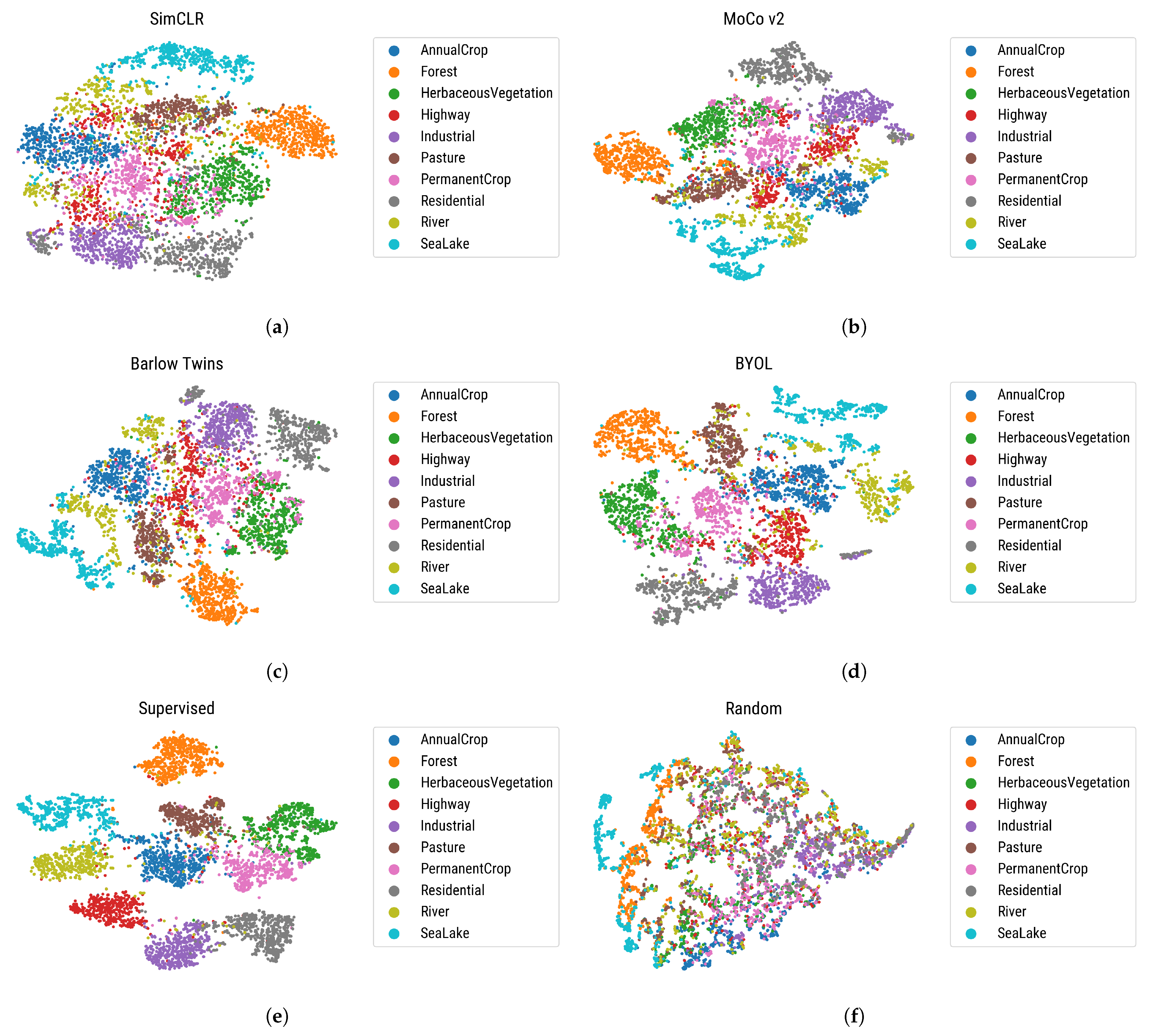
Figure 12SimCLR, MoCo-v2, BYOL, Barlow twinsEuroSATVisualize the pre-trained feature representations of different methods using t-SNE technique.
Table 5SimCLR, BYOLResisc-45, EuroSATEvaluate the individual impact of each commonly-used augmentation strategy in joint-embedding methods.
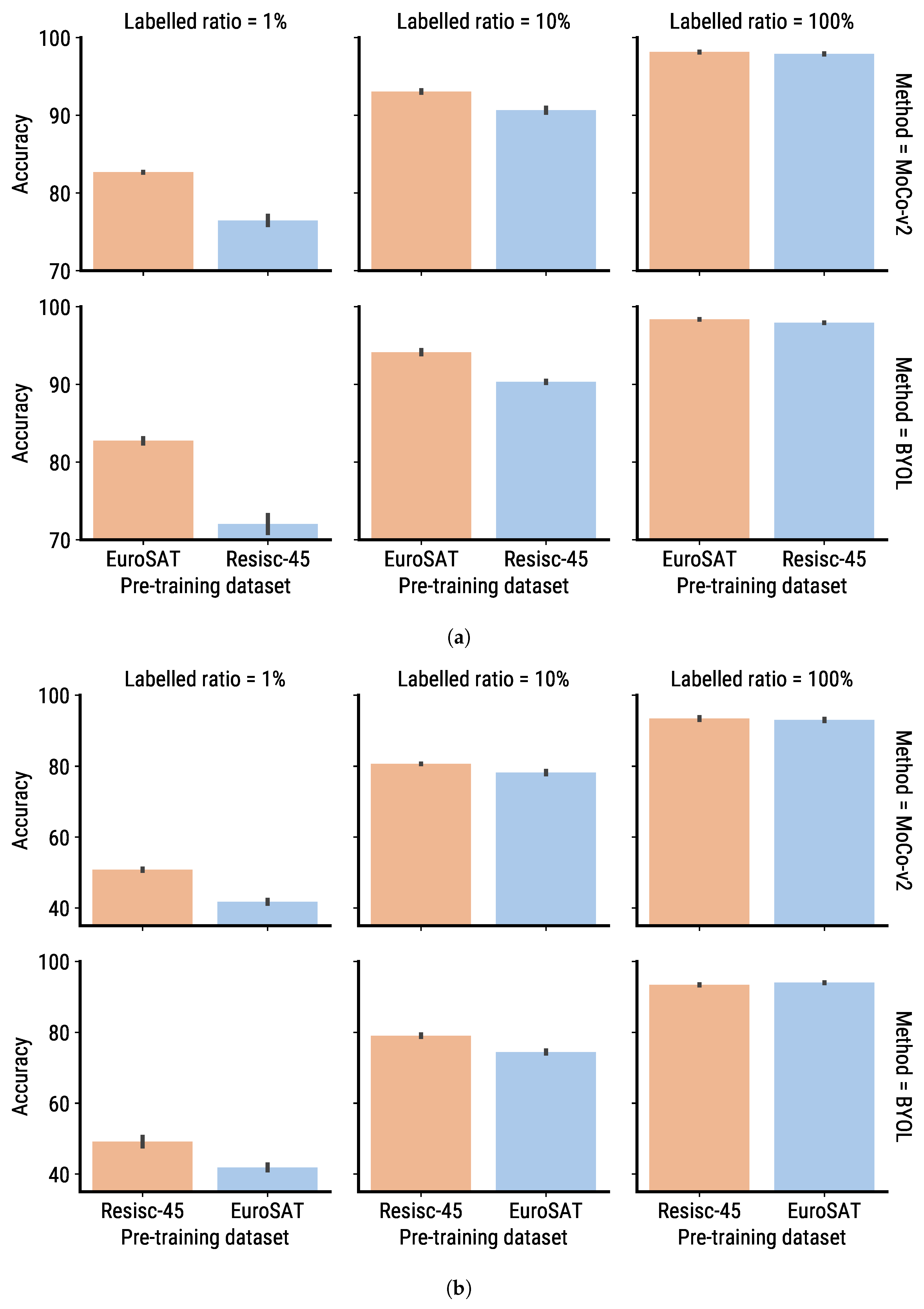
Figure 13MoCo-v2, BYOLResisc-45, EuroSATCompare the fine-tuning performance using pre-trained SSL models in two scenarios where the target dataset is the same as or different to the pre-training dataset.
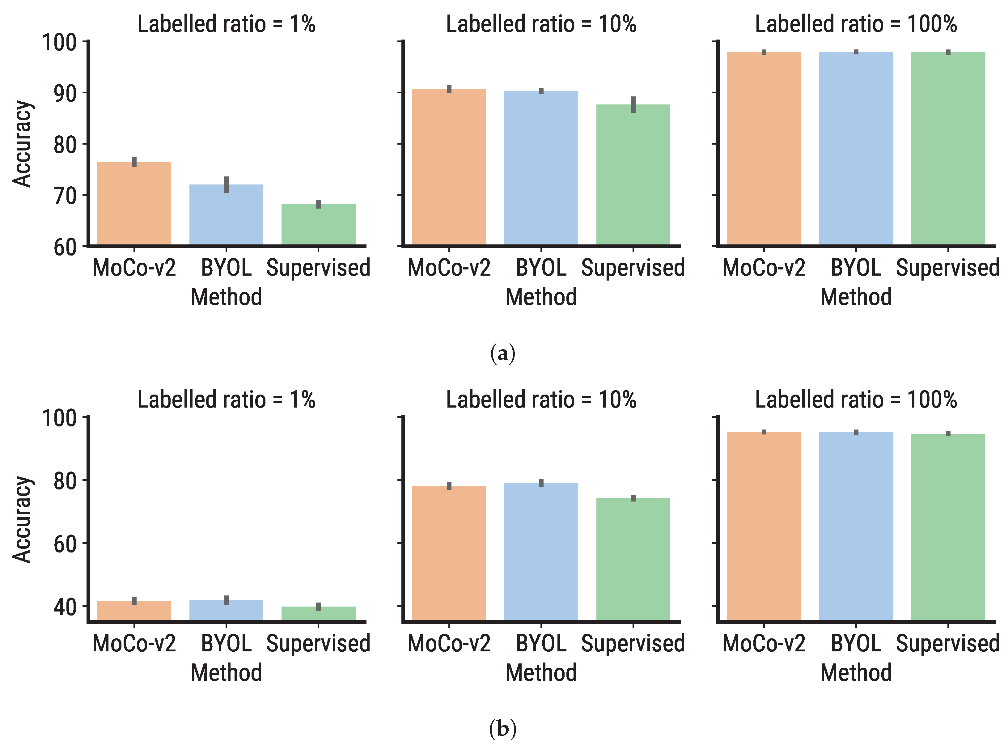
Figure 14MoCo-v2, BYOLResisc-45, EuroSATCompare the fine-tuning performance of supervised and self-supervised pre-trained models in a transfer learning scenario.
Table 3. Classification performance (accuracy and kappa coefficient) on the Resisc-45 and the EuroSAT datasets under the linear evaluation protocol (three runs).
Pre-Training MethodResisc-45EuroSAT
Acc. 100 × κ Acc. 100 × κ
Random initialization45.65 ± 0.8443.43 ± 0.8963.48 ± 0.1659.33 ± 0.19
ImageNet supervised90.32 ± 0.0089.93 ± 0.0094.46 ± 0.0093.84 ± 0.00
SimCLR [39]82.55 ± 0.6881.84 ± 0.7192.59 ± 0.0591.76 ± 0.05
MoCo-v2 [67]85.37 ± 0.1584.78 ± 0.1593.78 ± 0.0793.08 ± 0.08
BYOL [44]85.13 ± 0.0784.52 ± 0.3194.92 ± 0.1294.34 ± 0.13
Barlow Twins [48]83.14 ± 0.3082.44 ± 0.3195.59 ± 0.1795.08 ± 0.19
Table 4. Classification performance on the Resisc-45 and EuroSAT datasets under the fine-tuning evaluation protocol (three runs). Pre-trained models are fine-tuned with a limited number of labeled samples (1%, 10%, and 100%, respectively).
Pre-Training MethodResisc-45EuroSAT
1%10%100%1%10%100%
Random initialization32.39 ± 0.6967.68 ± 0.3991.05 ± 0.3253.64 ± 0.3876.76 ± 0.6796.49 ± 0.03
ImageNet supervised58.79 ± 0.2989.27 ± 0.2896.75 ± 0.0385.62 ± 0.2195.43 ± 0.1198.70 ± 0.02
SimCLR [39]41.14 ± 0.9478.22 ± 0.2593.01 ± 0.3277.46 ± 0.3892.04 ± 0.1597.62 ± 0.05
MoCo-v2 [67]50.83 ± 0.3980.71 ± 0.1693.45 ± 0.3882.67 ± 0.0693.06 ± 0.1898.15 ± 0.07
BYOL [44]49.30 ± 1.6478.92 ± 0.1193.39 ± 0.2082.74 ± 0.4394.15 ± 0.3598.36 ± 0.04
Barlow Twins [48]42.85 ± 1.2573.42 ± 0.9495.03 ± 0.2681.60 ± 0.4193.14 ± 0.1296.52 ± 0.10
Table 5. Ablation study on the augmentations using the linear performance. Experiments are conducted using SimCLR and BYOL.
Pre-Training MethodAugmentationsResisc-45EuroSAT
Gray ScaleColor JitterFlipCropAcc.Impr.Acc.Impr.
SimCLR [39] 46.14-50.52-
60.71+14.6061.50+10.98
67.79+7.0765.94+4.44
83.05+15.2791.52+25.57
BYOL [44] 40.74-61.52-
45.41+4.6764.19+2.67
54.08+8.6777.24+13.06
85.40+31.3194.54+17.30
Publisher’s Note: MDPI stays neutral with regard to jurisdictional claims in published maps and institutional affiliations.

