Article

Marine Gravimetry and Its Improvements to Seafloor Topography Estimation in the Southwestern Coastal Area of the Baltic Sea

1
Department of Surveying Engineering, School of Civil and Transportation, Guangdong University of Technology, Waihuanxilu 100, Guangzhou 510006, China
2
Department of Applied Earth Sciences, Faculty of Geo-Information Science and Earth Observation (ITC), University of Twente, Hengelosestraat 99, 7500 AE Enschede, The Netherlands
3
State Key Laboratory of Geodesy and Earth’s Dynamics, Innovation Academy for Precision Measurement Science and Technology, Chinese Academy of Sciences, Xudong Avenue 340, Wuhan 430077, China
4
School of Geodesy and Geomatics, Wuhan University, Luoyu Avenue 129, Wuhan 430072, China
5
Key Laboratory of Geospace Environment and Geodesy, Ministry of Education, Wuhan University, Luoyu Avenue 129, Wuhan 430079, China
*
Author to whom correspondence should be addressed.
Current address: Dipartimento di Ingegneria Civile ed Ambientale Sezione di Geodesia e Geomatica, Politecnico di Milano, Piazza Leonardo da Vinci 32, 20133 Milano, Italy.
Remote Sens. 2022, 14(16), 3921; https://doi.org/10.3390/rs14163921
Submission received: 9 July 2022 / Revised: 9 August 2022 / Accepted: 10 August 2022 / Published: 12 August 2022
(This article belongs to the Special Issue GRACE for Earth System Mass Change: Monitoring and Measurement)

Abstract

:
Marine gravimetry provides high-quality gravity measurements, particularly in coastal areas. After the update of new sensors in GFZ’s air-marine gravimeter Chekan-AM, gravimetry measurements showed a significant improvement from the first new campaign DENEB2017 with an accuracy of 0.3 / 2 = 0.21 mGal @ 1 km along the tracks, which is at the highest accuracy level of marine gravimetry. Then, these measurements were used to assess gravity data derived from satellite altimetry (about 3 mGal) and a new finding is that a bias of −1.5 mGal exists in the study area. Additionally, ship soundings were used to assess existing seafloor topography models. We found that the accuracy of SRTM model and SIO model is at a level of 2 m, while the accuracy of the regional model EMODnet reaches the lever of sub-meters. Furthermore, a bias of 0.7 m exists and jumps above 5 m in the SRTM model near the coast of Sweden. Finally, new combined gravity anomalies with sounding data are used to reveal the fine structure of ocean topography. Our estimated seafloor topography model is more accurate than existing digital elevation data sets such as EMODnet, SRTM and SIO models and, furthermore, shows some more detailed structure of seafloor topography. The marine gravimetry and sounding measurements as well as the estimated seafloor topography are crucial for future geoid determination, 3D-navigation and resource exploration in the Baltic Sea.

1. Introduction

The Baltic Sea, the largest shallow brackish water basin on the Earth, has a complicated seafloor topography [1,2]. Determining more refined seafloor topography would provide strategic and basic data for understanding the relevant tectonic structure and dynamic problems [3,4]. Currently, there are some problems existing in seafloor topography models and bathymetry data sets in this study area; e.g., the ship-sounding measurements are sparse in the Baltic Sea areas in the widely used global topography model SRTM (SRTM15+ [4]). Additionally, the global topography model (e.g., GEBCO2020 [5]) of the General Bathymetric Chart of the Oceans provides a global terrain model for ocean and land with a spatial resolution of 15 . The grid uses as a “base” Version 2 of the SRTM15+ data set [4]. This data set is a fusion of land topography with measured and estimated seafloor topography. However, it still lacks information about the contributed data sources and depths assigned to grid cells in some areas interpolated from sparse depth data from charts in the Baltic Sea. There are also regional seafloor topography databases, e.g., the Baltic Sea Bathymetry Database (BSBD, the high-resolution data are not available for download) and the digital terrain model of the European Marine Observation and Data Network (EMODnet) [6]. The EMODnet model was based on three types of bathymetric data sources: The first includes bathymetric surveys, such as single and multibeam surveys, echo soundings and even historic leadline soundings. These bathymetric survey data sets are the preferred data sources because of their high resolution. The second includes composite data sets, which include a set of surveys merged and gridded altogether. The third includes gaps with no data coverage that were completed by integrating the worldwide GEBCO Digital Bathymetric grid. The lack of coverage was filled by coarse resolution (up to several kilometers) information extrapolated from altimetry measurements for satellites [4,6]. This problem is rather restricted to the Baltic Sea (deep oceans as well due to data gaps of bathymetric measurements) because of legal restrictions regarding high-resolution bathymetric information, specifically an issue in Sweden and Finland [7]. In the southwestern area of the Baltic Sea, several countries (e.g., Denmark, Germany, Poland and Sweden) have measured seafloor topography. Therefore, several bathymetric data sets exist for the Baltic Sea area, each with its advantages and drawbacks, and none are ideally suited for a wide range of applications, e.g., different accuracy, spatial resolution, vertical data and so on [6,8]. In addition, the common data sets with rather low detail resolution are not sufficient for many tasks as high-quality bathymetry data are missing in many areas, and further mapping activity is needed [8]. Small ship-sounding data gaps remain in these regional databases or models, as shown in the relevant survey tracks in the EMODnet model (tracks can be accessed from the website: https://portal.emodnet-bathymetry.eu/?menu=19, last accessed on 10 January 2022).
Coincidently, high-precision marine (or airborne) gravimetry has been proven to estimate refined seafloor topography, which is the efficient way to obtain Earth gravity field information at short wavelengths, especially in coastal and offshore areas compared to other technical methods, e.g., satellite gravimetry, satellite altimetry and terrestrial gravimetry (e.g., [9,10,11,12,13,14,15,16]). In the Baltic Sea, marine gravity has been measured in different regions with different levels of precision. Denker and Roland [17] compiled and evaluated the marine gravity data set surrounding Europe. The root mean square (RMS) of the gravity differences at crossover points was 15.5 mGal and became 4.70 mGal after adjustments [17] (1 mGal = 10 5 ms 2 ). Hunegnaw et al. [18] analyzed the marine gravity data set in the northern Atlantic Ocean, and the unweighted standard deviation of the cross-over errors was 4.03 mGal and reduced to 1.58 mGal after network adjustment. When data were weighted, the standard deviation reduced from 1.32 to 0.39 mGal. Lequentrec-Lalancette et al. [19] computed a standard deviation value of 3.60 mGal from the differences at crossover points in the Mediterranean. Apart from that, the RMS of cross-over errors in military trials with a type of gravity sensor (commercially available) was only 0.10–0.20 mGal in rough seas [18] while Bell and Watts [20] showed cross-over errors of ±0.38 mGal using a BGM-3 sea gravimeter. However, the precision of marine gravity anomalies did not match this precision at that time for different reasons [18]. Thus, it is of importance to conduct more precise marine gravimetry in the Baltic Sea.
In this circumstance, German Research Centre for Geosciences (GFZ) performed several marine gravimetry missions in the Baltic Sea since 2013 to improve the local geoid in German coastal areas. Marine gravimetry campaigns were also implemented by GFZ to verify and check the quality of the existing gravity data and to fill data gaps to develop a high-quality geoid model in the entire Baltic Sea, which are part of the project “Finalising Surveys for the Baltic Motorways of the Sea” (FAMOS) [16]. In addition, these marine gravimetry measurements could also be used to estimate seafloor topography. Together with the gravimeter, a single-beam sonar system comprising Kongsberg EA400 Vertikallot was also installed onboard the research vessels to obtain ship-sounding measurements directly with high-precision and high-spatial-resolution using commercial software [21,22]. However, these ship-sounding data were only measured in part of the gravimetry campaigns instead of covering each gravimetry track as the original aim was to use these ship-sounding data in some particular cases [16]. In this case, new combined gravity anomalies (satellite altimetry and marine gravimetry) and ship-sounding data have complementary advantages including uniformed coverage and high precision directly measured in specific points, respectively. Therefore, they could be applied together to reveal the fine structure of the seafloor topography by the gravity-geologic method (GGM) in the southwestern coastal area of the Baltic Sea (longitude: 11 15 ; latitude: 54 56 ), including parts of the central European system, the Torne European Suture Zone and the Ringkobing-Fyn High, one of the most attractive areas showing complicated geological structure caused by different tectonic events [2]. The following sections will present a more detailed explanation and analysis of marine gravimetry and seafloor topography estimation.

2. Materials and Methods

2.1. Marine Gravimetry Data Processing

The main equipment used in these marine gravimetry campaigns is a mobile air-marine gravimeter Chekan-AM. It is designed as a double quartz elastic system (two quartz torsion fibers) mounted on a GNSS-supported and gyro-stabilized platform [23,24]. The basic equation to calculate the gravity value from marine gravimetry campaigns based on the gravimeter Chekan-AM’s raw measurements is shown in Equation (1) [15,16]:
g = g Chekan + δ g Etvs δ g HAC δ g drift + δ g link
where g C h e k a n is the raw gravity measurement from the Chekan-AM gravimeter, δ g E t v s is the E o ¨ t v o ¨ s correction, δ g H A C is the horizontal acceleration correction, δ g d r i f t is the instrumental drift correction, and δ g l i n k is the difference between the reference gravity value and the measurement of Chekan-AM at the base station. The exact equation for the Chekan-AM gravimeter value is as follows:
g C h e k a n = b × ( m m 0 ) + a × ( m m 0 ) 2 + T g × ( ( b × ( m m 0 ) + a × ( m m 0 ) 2 ) t )
where a, b, m 0 and T g are constants determined during Chekan-AM’s calibration and m is the sum of the recordings of the two sensors m 1 and m 2 . Here, the new values for the constants (measured after the gravimeter Chekan-AM was updated with new sensors by the manufacturer) are presented in Table 1 with the previous values.
Following the raw gravity measurement in Equation (1), δ g E t v s is the E o ¨ t v o ¨ s correction that is calculated based on the trajectories of the research vessels (or ferries) (e.g., [15,25,26]). To determine kinematic trajectories, the GNSS L1 carrier phase observations from GPS receivers (JAVAD Delta G3T) are used in Differential GPS (DGPS) method because of the low noise. Li et al. [27] and Lu et al. [16] tested that the precision of 1–2 cm in the horizontal and 1–5 cm in the vertical directions can be obtained with DGPS by applying multi-GNSS systems in the WGS 84 reference system. The GNSS observations help determine the positions of the gravimeter Chekan-AM and the sonar system Kongsberg EA400 Vertikallot. In some special cases, such as the squat effect, seiches, the GNSS-derived kinematic vertical acceleration can help reduce such influences in marine gravimetry [16]. In addition, GNSS kinematic vertical positions help reduce such influences in ship sounding when bathymetric depths are uniformed to the same vertical datum, e.g., geoid. δ g H A C is the horizontal acceleration correction as horizontal components also influence vertical accelerations.
In our study, the low-pass filter based on the fast Fourier transform (FFT) was applied to Chekan-AM measurements, E o ¨ t v o ¨ s corrections and horizontal acceleration corrections to filter out noisy components [28]. The main advantage is that the low-pass filter based on FFT—characterized by the cut-off wavelength, the transition region and the shape of the transfer function—can be defined directly in the frequency domain. The main parameter of the low-pass filter is the cut-off wavelength, which corresponds to the resolution of the final gravimetry results. The length of the transition zone is related to the oscillations of the unit impulse response of the low-pass filter [29,30]. The transition zone should not be too short. In other words, the oscillations of the unit impulse response should not be very large. Here, the cutoff period and the length of the cosine type transition zone are 400 s and 120 s (30% length of the cutoff period) based on the practical method [16]. The transfer function of the low-pass filter in the frequency domain can be found in our previous studies [15,16]. A more detailed processing scheme of marine gravimetry with the gravimeter Chekan-AM can be found in the operation manual from the manufacturer and has been shown previously (e.g., [14,15,16,31,32,33,34,35]).

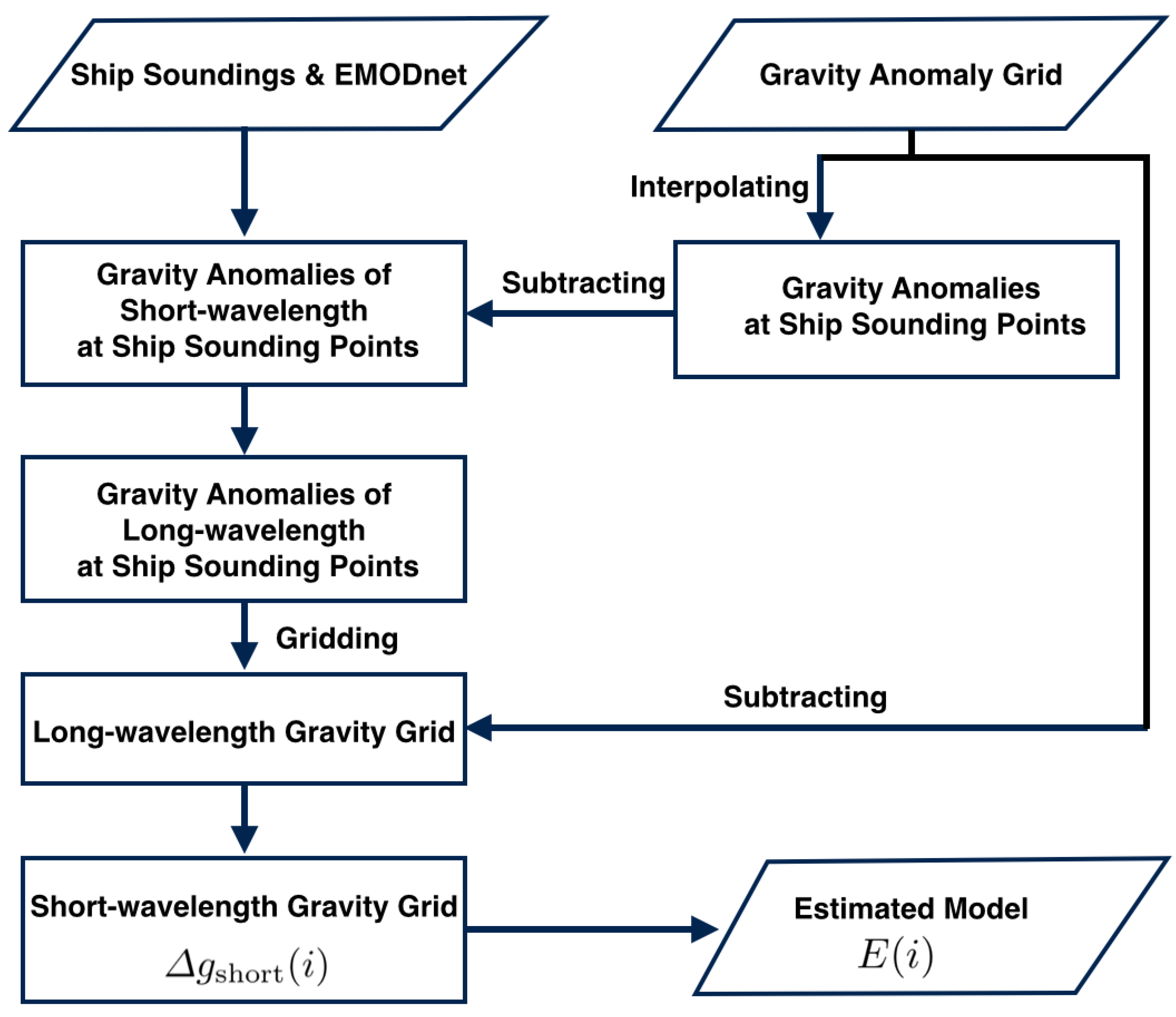
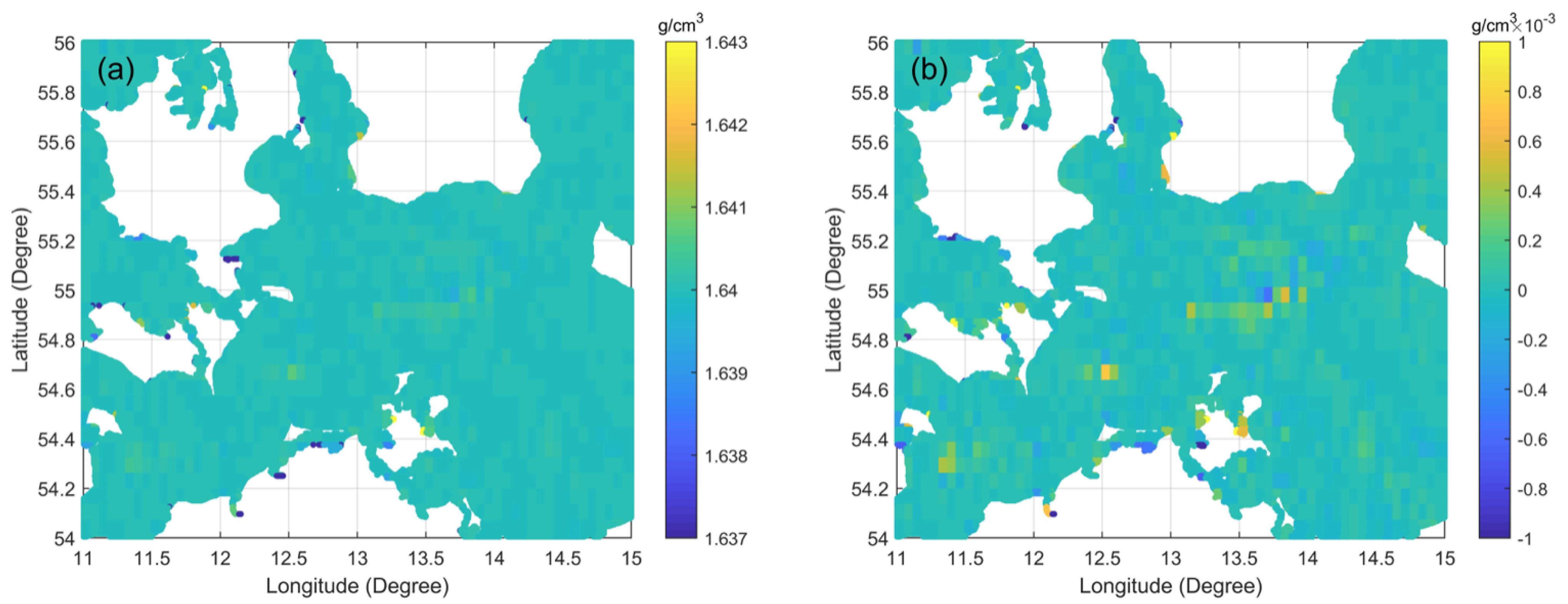
2.2. Seafloor Topography Estimation

The main methods of using gravity anomaly to retrieve seafloor topography include Smith and Sandwell method, gravity-geological method (GGM), admittance method, simulated annealing method and the nonlinear iterative least squares method (e.g., [36,37,38,39,40,41,42]). Among them, the GGM has high inverted precision and is suitable for areas with relatively uniform ship-sounding data as control points. This method has been used in both coastal and offshore areas. Therefore, the GGM was used to determine the seafloor topography of the Baltic Sea from gravity anomalies and ship-sounding data in this paper. This method was first developed by [43] to predict the depth to basement overlain by lower density glacial drift deposits and then used to determine the seafloor’s topography. In the GGM, the graivty anomaly Δ g obs ( i ) on the geoid can be regarded as two parts:
Δ g obs ( i ) = Δ g short ( i ) + Δ g long ( i )
where Δ g short ( i ) is the short-wavelength gravity anomaly, which is caused by seafloor topography; Δ g long ( i ) is the long-wavelength gravity anomaly, caused by deep inhomogeneous materials; i is the location of gravity anomaly grid. The short-wavelength gravity anomaly Δ g short ( j ) at control points (existing ship-sounding data) can be derived from the Bouguer plate formula:
Δ g short ( j ) = 2 π G Δ ρ ( E ( j ) D )
in which G is the gravitational constant, 6.672 × 10 8 cm 3 g 1 s 2 . Δ ρ is the density contrast between seawater and bedrock, assumed as 1.64 g/cm 3 . However, based on many experiments, the real value of Δ ρ is different from 1.64 g/cm 3 , which is usually determined by the iteration method [38]. In this study, Δ ρ is achieved by the iteration of linear relation between short-wavelength gravity anomaly and depths of control points at different gridded regions. When the difference of twice Δ ρ is less than the preset threshold value, the iteration is stopped and the optimal Δ ρ is outputted. j is the location of control point; E ( j ) is the known depth of control points; D is the reference datum elevation, which is generally set as the deepest depth of the control points. According to Equations (3) and (4), the long-wavelength gravity anomaly Δ g long ( j ) at control points can be calculated by the following:
Δ g long ( j ) = Δ g obs ( j ) Δ g short ( j )
where Δ g obs ( j ) is the gravity anomaly of control points, interpolating from Δ g short ( i ) . After gridding Δ g long ( j ) , Δ g long ( i ) will be obtained. Inserting Δ g long ( i ) into Equation (3), Δ g short ( i ) can be determined. Based on Equation (4), the estimated seafloor topography model E ( i ) is derived from the following.
E ( i ) = Δ g short ( i ) 2 π G Δ ρ + D
The flowchart clearly presents the data-processing progress of this methodology in Figure 1. In order to test this methodology, we conducted an experiment to analyze the contribution of marine gravimetry data to the estimation of the seafloor topography, as shown in Appendix A. The results showed that the precision of the seafloor topography is at a level of 2 m estimated from combined gravity anomalies by the GGM. The final step is to take base map E ( i ) in combination with ship-sounding data (control points) using a minimum curvature gridding algorithm as the ship-sounding data containing the high-precision and high spatial-resolution information of the seafloor’s topography [4,37,44]. A more detailed methodology of the GGM is presented by former research (e.g., [3,38,45,46]).

3. Results

3.1. Marine Gravimetry Results

Before 2017, five marine gravimetry campaigns onboard different research vessels were carried out in this project with an precision of 0.50 mGal along tracks without adjustments (the RMS of gravity differences at 380 crossover points was 0.76 mGal) [16]. The sub-mGal is more precise than previous marine gravimetry data sets with the precision of several or even tens of mGal, as mentioned above [17,18,19]. However, a sudden gravimeter drift change of about −7.00 mGal occurred because of a heavy storm during the DENEB2015 campaign (DENEB is the name of the research vessel used in the gravimetry campaign). Moreover, an abnormal gravimeter drift (−2.50 mGal/day) was obtained from the gravity measurements in the harbors in the next DENEB2016 campaign. The gravimeter drift should be a positive value under normal conditions. GFZ implemented two marine gravimetry campaigns within the project FAMOS in 2017. One of the campaigns was onboard the research vessel DENEB (Figure 2a) from 9 July to 20 July near the coast of Germany, Poland and Sweden. The other testing campaign was the first time that the gravimeter was implemented on the ferry URD (Figure 2c) instead of the research vessels from 6th October to 14th October between the harbor Travem u ¨ nde and Liepaja. The primary purpose was to test if it could implement marine gravimetry campaigns on large ferries to measure long repeat tracks and whether it can save expenses simultaneously.
Here, we present the latest marine gravimetry results using the updated gravimeter Chekan-AM in the study area. First, we analyzed the drift of the gravimeter. Then, we compared the gravimetry tracks in different missions. Finally, we presented the overall precision of the marine gravimetry by checking crossover points.

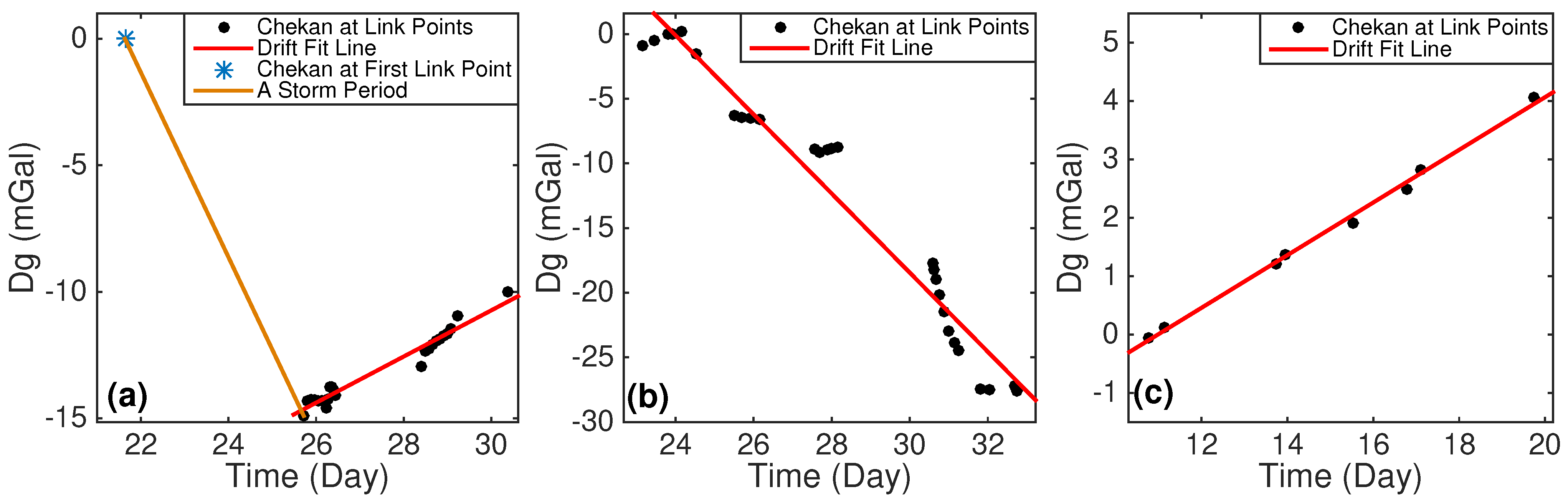
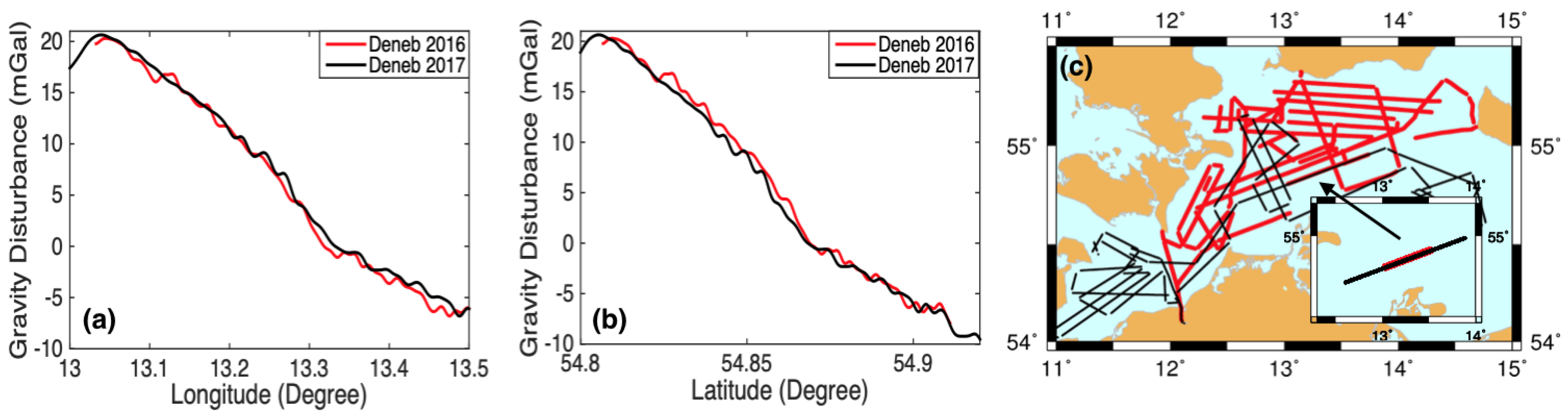
3.1.1. Drift Improvement

As mentioned above, some problems in the drift determination existed according to the Chekan-AM measurements at link points (in harbors) before 2017. Figure 3a shows a negative shift of 15.00 mGal in drift between the first link point and the next one in the campaign DENEB2015 because of a storm during this period. We checked gravity differences at two crossover points between the track during the storm and the track before the storm. The gravity differences at these two crossover points were, respectively, 7.49 and 6.03 mGal. Therefore, something definitely happened to the gravimeter Chekan-AM because of the strong shaking of the ship in the storm. Apart from that, the drift of DENEB2016 was negative and unstable (−2.50 mGal/day), as shown in Figure 3b. With the updated gravimeter Chekan-AM, the drift in the campaign DENEB2017 was very stable with a normal value of 0.50 mGal/day, as shown in Figure 3c. Furthermore, the gravimetry measurements of the campaign URD2017 (also another campaign Finnlady2018) implemented on ferries also had a very stable drift [47,48].

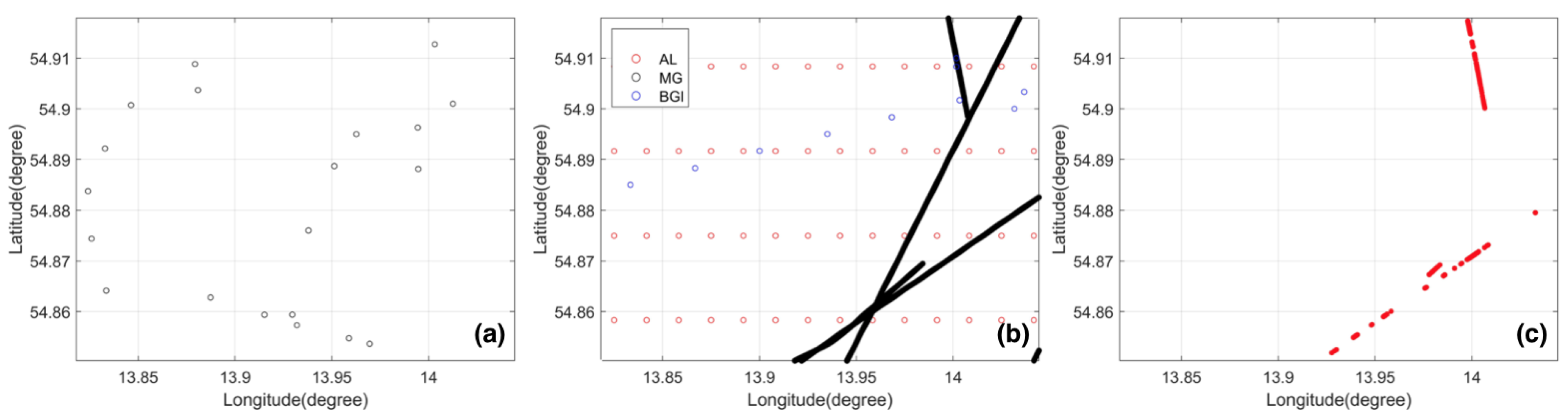
3.1.2. Tracks Checking

Here, the measurements of a typical track from the campaign DENEB2017 are shown in Figure 4. The range of the raw shipborne gravimetry measurements extends to ± 20 Gal (see Figure 4a) because of the other kinematic vertical accelerations (treated as noise). Fortunately, these disturbing signals in Chekan-AM raw measurements are mainly concentrated in high frequency areas, as shown in Figure 4c, and they can be removed by applying the FFT low-pass filter, as mentioned above. The filtered measurements are several tens of mGal (see Figure 4b) as expected of gravity variations in the Baltic Sea, e.g., from the gravity field models.
Furthermore, we checked two repeat tracks between campaigns DENEB2016 and DENEB2017, as shown in Figure 5c. Because the distance between these two tracks is within 50 m and the spatial resolution is approximately 1 km (half-wavelength), these two tracks can be treated as repeat tracks. Figure 5a,b, respectively, show the gravity disturbances of the repeat tracks along with longitude and latitude directions. These two sub-figures show that the gravity disturbances of the track from DENEB2017 are a little smoother than those of the track from DENEB2016.

3.1.3. Crossover Points Checking

To demonstrate the overall precision of these three campaigns, Table 2 presents the gravity differences at the crossover points. The precision of DENEB2016 is the worst with the largest Min (0.84 mGal), MAX (1.73 mGal), Mean (0.11 mGal) and RMS (0.55 mGal) values compared to the other two campaigns. This campaign was influenced by the negative (abnormal) and unstable drift. Compared with this campaign, the precision of DENEB2015 is slightly improved. However, there was a large storm that happened during the campaign. The raw measurements of the gravimeter Chekan-AM had a sudden jump of several mGal and continued with a negative drift for a period of time. We applied a fit drift model f ( t ) = 0.8215 t 3 + 4.697 t 2 11.21 t 3.052 for the storm period according to the gravity differences at crossover points. Here, parameter t in the drift model represents the time of day, and the crossover points are between the normal tracks and the tracks in the storm period. Otherwise, the Max and RMS of gravity differences at crossover points are 19.00 mGal and 10.16 mGal. After the gravimeter Chekan-AM was updated, the first campaign of DENEB2017 showed significant improvements: The absolute values of Min (−0.76 mGal) and Max (0.52 mGal) of gravity differences at crossover points were within 1.00 mGal, and the RMS value reached 0.30 mGal, which is close to the current claimed the highest precision of 0.10–0.20 mGal. In addition, the gravimetry measurements of the campaign URD2017 (also another campaign Finnlady2018) implemented on ferries were at the precision level of 1.00 mGal along the tracks [47,48].

3.2. Seafloor Topography Estimation Results

After obtaining the high-precision and high-resolution marine gravimetry data in the southwestern coastal area of the Baltic Sea, they were applied to estimate the seafloor topography for revealing a more detailed seafloor structure. First, these marine gravimetry data helped in checking the precision of gravity anomalies derived from satellite altimetry, and then they were combined into new gravity anomalies with the weights based on their precision. The reason was that the latter provides a good and uniform gravity data coverage in the ocean but generally lower precision in the coastal areas. Second, the ship-sounding data were used to check the precision of existing digital terrain models and helped find the best initial model as part of the control points for the seafloor topography estimation in the GMM method. Finally, the seafloor topography was estimated to reveal a more detailed seafloor structure based on the data sets mentioned above. These research details can be found in the following subsections.

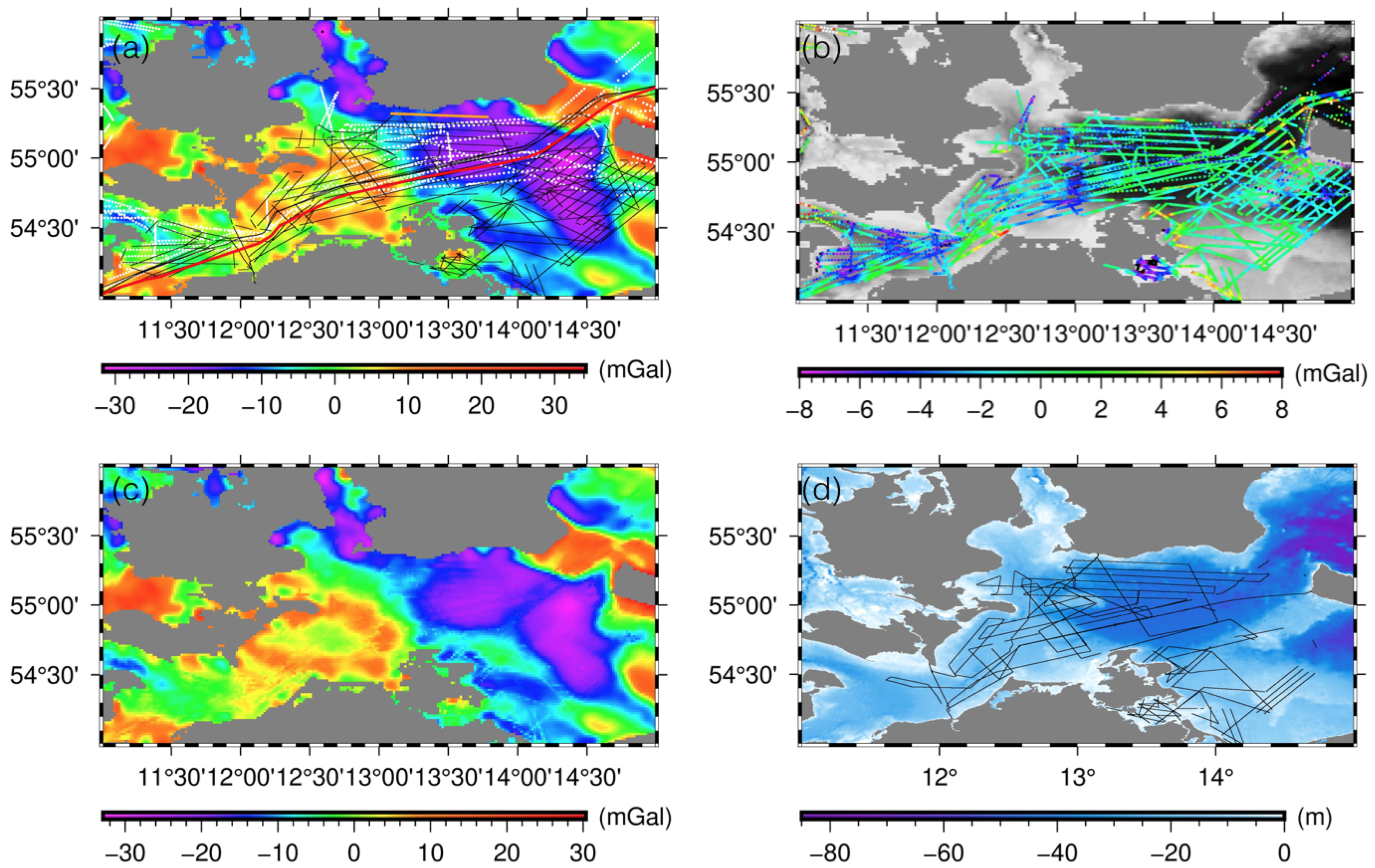
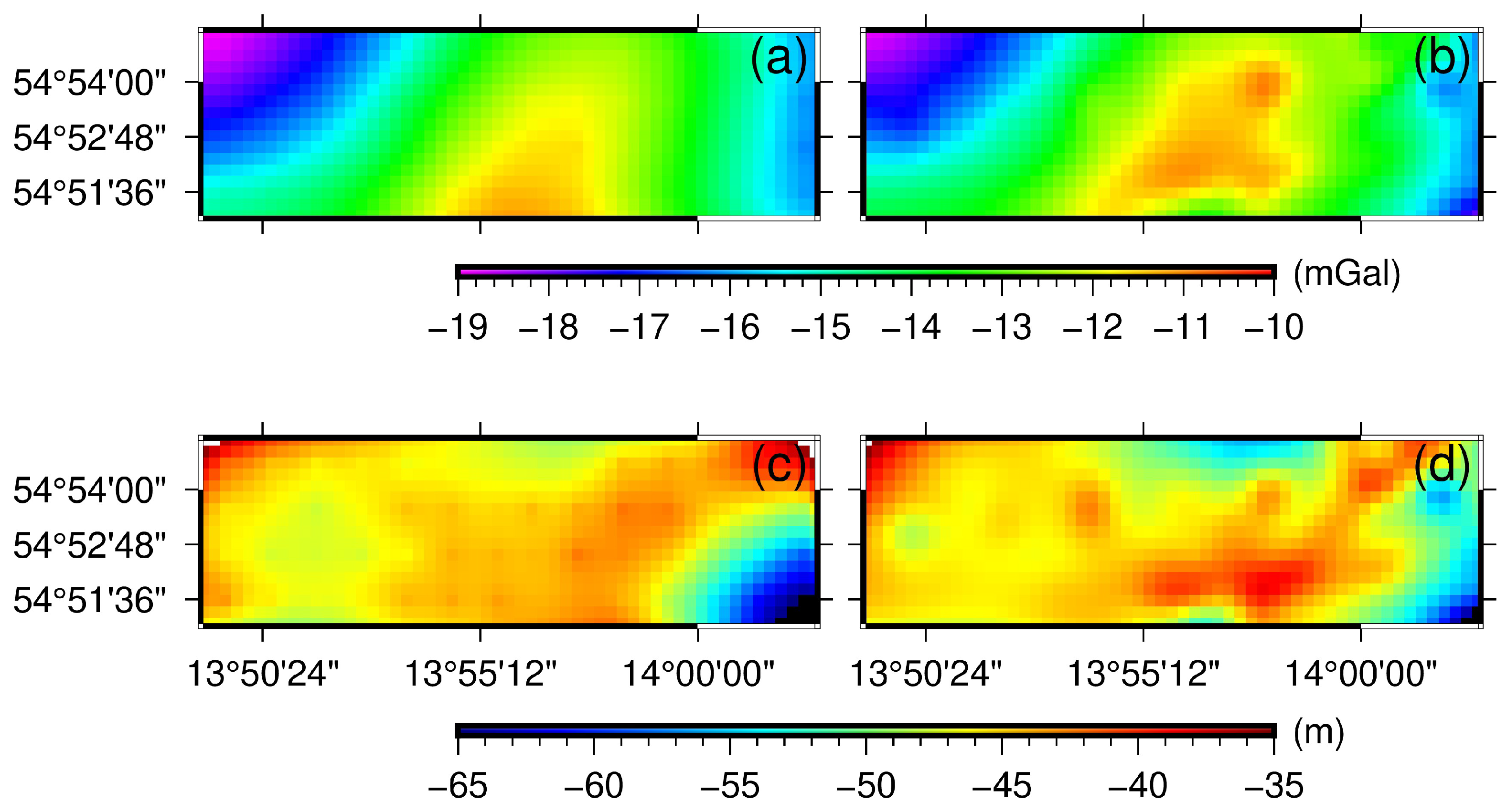
3.2.1. Checking and Combining Different Gravity Anomalies

The gravity anomalies from satellite altimetry (2.00–3.00 mGal @ 1 ) provide a good gravity data set for seafloor topography estimation [49]. This data set (the latest version of V31.1) can be downloaded from the Scripps Institution of Oceanography [50]. These gravity anomalies from this data set are shown in Figure 6a in the southwestern coastal area of the Baltic Sea. However, compared with marine gravimetry, the precision is relatively lower in coastal areas [51]. Furthermore, there are islands in the western part of the Baltic Sea and a few narrow straights, introducing unreliable altimetry results in some areas. On the other side, the gravity anomalies from marine gravimetry have a better spatial resolution and precision (0.20–1.00 mGal @ 15 ) and can be used to assess the quality of the gravity data derived from satellite altimetry. The white points represent the marine gravimetry measurements from the International Gravimetric Bureau (BGI) while the black tracks represent our marine gravimetry tracks.
The gravity differences between satellite altimetry and marine gravimetry were calculated after interpolating the gravity anomalies in the locations of marine gravimetry from the satellite altimetry gravity anomalies using the cubic spline interpolation method, as shown in Figure 6b. The main gravity differences exist near the coastal areas, islands, and narrow straights. From Table 3, the mean and RMS values of the differences between BGI’s marine gravity anomalies and that interpolated from SIO’s altimetry gravity anomalies are −1.95 mGal and 3.71 mGal. In addition, the mean and RMS values of the differences are −1.52 mGal and 2.59 mGal between our marine gravity anomalies and those interpolated from SIO’s altimetry gravity anomalies. Therefore, it can be concluded that the precision of satellite altimetry gravity anomalies is about 3.00 mGal, and a systematic offset of −1.50 mGal exists in this data set within this research area. Therefore, we removed this systematic offset before combining these different gravity anomalies from our marine gravimetry, BGI’s marine gravimetry, and SIO’s altimetry data sets in seafloor topography estimation.
As the next step, these different gravity anomalies were interpolated to create a grid of the observed gravity anomalies in a spatial resolution of 15 by using a minimum curvature gridding algorithm in Figure 6c [44,52]. The weights of our marine gravity anomalies, BGI’s marine gravity anomalies, and SIO’s altimetry gravity anomalies in the interpolation were determined according to these different data sets’ precision (0.50 mGal, 2.60 mGal and 2.60 mGal). Here, the reasons to set the same value of 2.60 mGal for BGI’s marine gravity anomalies and SIO’s altimetry gravity anomalies were as follows: First, there is no information on the precision of the BGI’s marine gravity data, and the precision is relatively low, which was obtained mainly in 1970–1980s of the last century. Second, the RMS of the differences between BGI’s marine gravity anomalies and that interpolated from SIO’s altimetry gravity anomalies is 3.70 mGal. In comparison, it is 2.60 mGal between our total marine gravity anomalies (precision of 0.50 mGal) and interpolated from SIO’s altimetry gravity anomalies. In Figure 6c, the gravity anomalies range from approximately −32.00 mGal to 30.00 mGal. They reflect all anomalous materials, which contain signals from the undulation of seafloor topography. For example, in the ocean center, the distribution pattern of negative gravity anomalies is similar to that of the seafloor’s topography (see Figure 6d). Therefore, our new combined high-precision gravity anomaly was applied to estimate the seafloor topography to reveal a more detailed seafloor structure in this study area.

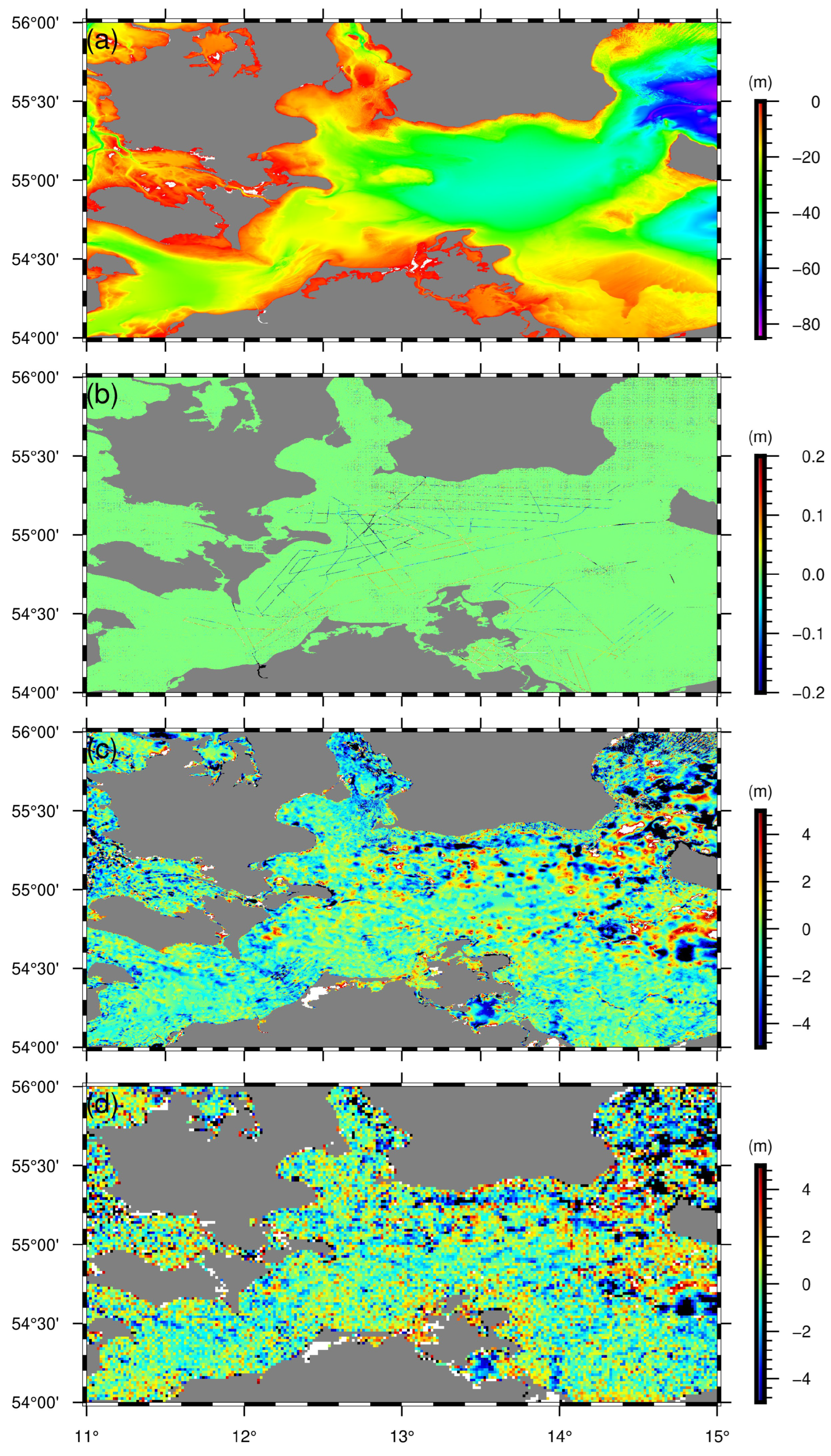
3.2.2. Checking Existing Digital Terrain Models

With marine gravimetry onboard the research vessels in the Baltic Sea, a sonar system (Kongsberg EA400 Vertikallot, at 38/200 kHz) obtained the ship-sounding data with a high-spatial-resolution of several meters. Here, sound velocities were calculated using three parameters: conductivity (C), temperature (T) and depth (D) via pressure. They were measured by a so-called CTD profiling probe. A mean value is then used in EA400 to correct for sound-speed errors in real time. An in-house software development named WinProfile Sharp was used for data acquisition and processing. The precision of the ship-sounding data is 0.15 m based on 412 cross-over points of the black tracks in Figure 6d. It reaches the current precision level of sub-meters in shallow waters. Furthermore, an external verification with respect to the measured ship-sounding data was applied by comparing them to the available ship-sounding data from the EMODnet model (downloaded from the website: https://www.emodnet-bathymetry.eu/search, last accessed on 10 January 2022). The Min, Max, Mean and STD values of the differences from 2640 points were −2.46 m, 1.91 m, −0.20 m and 0.32 m, respectively. The results confirmed that there was no obviously bias in the measured ship-sounding data at a high precision level.
In addition, there are several globally and regionally digital elevation data sets or models with different spatial resolution, e.g., the SRTM model ( 15 spatial resolution, vertical datum based on the geoid derived from the gravity field model EGM96), the SIO model (V20.1, 1 spatial resolution, vertical datum based on the geoid derived from the gravity field model EGM2008, Smith and Sandwell [36]) and the EMODnet model (about 4 spatial resolution and vertical datum based on the lowest astronomical tide) in this research area. Here, EGM2008 is a spherical harmonic model of the Earth’s gravitational potential as a replacement of EGM96 developed by a least squares combination of the ITG-GRACE03S gravitational model and its associated error covariance matrix, with the gravitational information obtained from a global set of area-mean free-air gravity anomalies defined on a 5 arc-minute equiangular grid [53]. The highly accurate long wavelength information provided by GRACE data would be complemented with the short wavelength information contained within the 5 arc-minute gravity anomaly data. ITG-GRACE03S is based on GRACE Satellite-to-Satellite Tracking (SST) data acquired during the 57-month period from September 2002 to April 2007. No other data were used in its development, which followed the short-arc analysis approach. This GRACE-based gravity field model is complete with respect to a spherical harmonic degree and order 180, and it was made available accompanied by its fully occupied error covariance matrix [54,55]. In addition, the SRTM model is combined with ship-sounding data on the base of the SIO model [4,36]. Therefore, we can assess the quality of these different data sets and models based on the measured ship-sounding data in this coastal area. Before performing such assessments, these different data sets and our ship-sounding data were uniformed to the same vertical datum of the SIO model (the geoid derived from the gravity field model EGM2008) [53,56,57,58]. Here, the uniformed vertical datum could also be transformed to the geoid derived from the latest gravity field models, e.g., EIGEN-6C4 or future uniformed local geoid in the Baltic Sea area, which contain the latest satellite gravimetry data from the Gravity Recovery And Climate Experiment (GRACE), Gravity field and steady-state Ocean Circulation Explorer (GOCE), as well as GRACE-FO (e.g., [59,60,61,62,63,64,65]). For example, the RMS of geoid differences between EIGEN-6C4 and EGM2008 is 3 cm in this study area.
The depth differences between ship-sounding data and existing models were calculated after interpolating the depth in the locations of ship-sounding data from these models. The depth differences between the EMODnet model and SRTM model (or the SIO model) were calculated by interpolating to the same spatial resolution of 15 ( 1 for the SIO model). From Table 4, the RMS of the differences between the EMODnet and SRTM models (or the SIO model) is about 3.00 m. According to the assessment of different models by ship-sounding data, the precision of the SRTM model and SIO model is at a level of 2.00 m in these coastal areas, and the regional model EMODnet with a high spatial resolution reaches the precision level of sub-meters. The depth differences between these three models in different spatial resolutions confirm that the precision of global model SRTM (and SIO) is at a level of 2.00–3.00 m in the entire southwestern part of the Baltic Sea. We also found that the mean values of the depth differences were obviously larger between the SRTM model and the other two models (EMODnet and SIO) and the ship-sounding data. Therefore, a mean difference of about 0.70 m may exist in the SRTM model in this area. These data help fill some ship-sounding data gaps in the southwestern coastal areas.

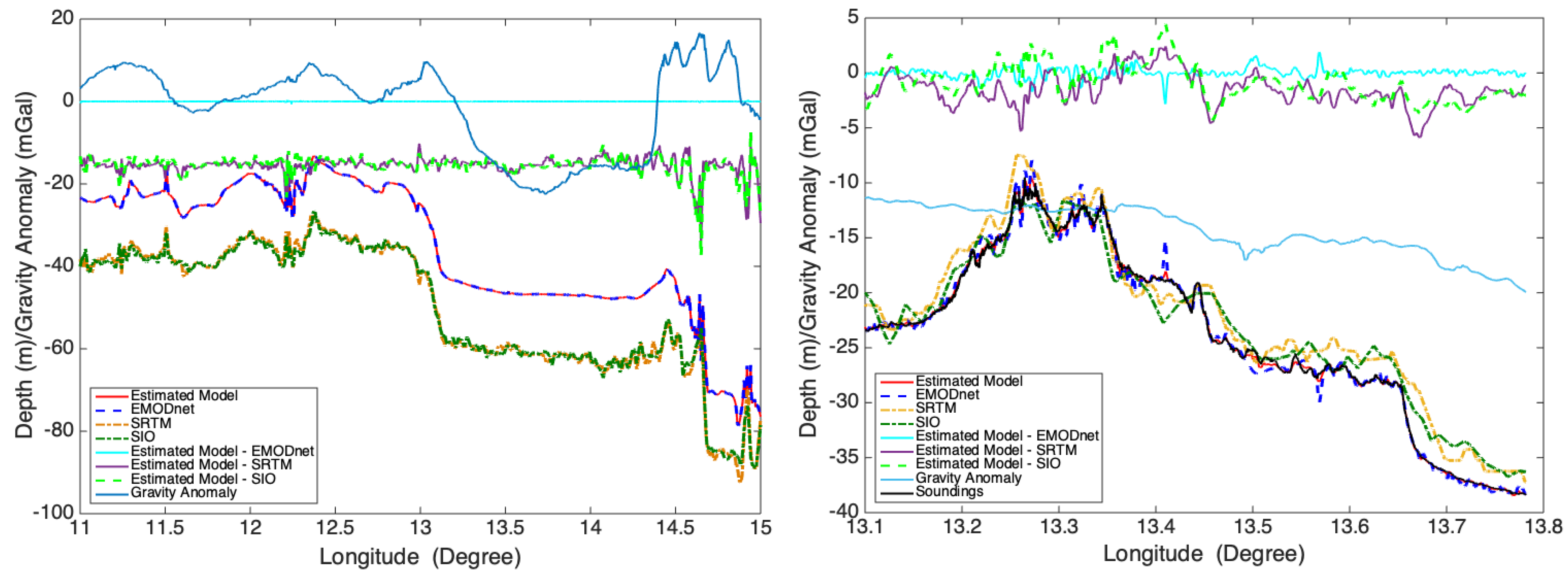
3.2.3. Revealing the Fine Structure of Seafloor Topography

Based on the assessments and findings as mentioned above, the GGM was used to reveal the fine structure of seafloor topography in the southwestern coastal area of the Baltic Sea, as shown in Figure 7a [52], where D was set as −82 m, the threshold value for the iteration of Δ ρ was 1.0 × 10 3 g/cm 3 and the resolution of gridded regions was 15 . Due to dense control points, only after one iteration did the RMSs of the differences between Δ ρ and the initial Δ ρ reach 5.9545 × 10 4 g/cm 3 , which were smaller than the threshold value. Therefore, the final Δ ρ was determined as shown in Figure 8a, and the corresponding error was shown in Figure 8b. The final determined Δ ρ was around 1.64 g/cm 3 , and the errors were at the level of 1.0 × 10 4 g/cm 3 , which were very small. Furthermore, the RMS between inverted seafloor topography and that of control points was calculated, which was 0.76 m. It indicated that the Δ ρ determined in this paper was reasonable. In this article, the topography model EMODnet in a spatial resolution 4 and 80% of the ship-sounding data were used as control points, and 20% of the ship-sounding data were used as checkpoints. We combined the EMODnet model and our ship-sounding data because of the high precision of ship-sounding data and good data coverage of the EMODnet model. These control points were first interpolated in a grid with a spatial resolution of 15 , which is the same as the spatial resolution of the combined gravity anomalies mentioned above. These two data sets were used as the depth’s input signals in seafloor topography estimations. The final step was to interpolate the estimated seafloor topography together with the control points into a final grid with a spatial resolution of 4 .
From Figure 7a, the deepest seafloor exceeds 80 m, which is located northeast of the study area. In the center areas, the depths of the seafloor change gently, and they are primarily concentrated at approximately 40 m. In contrast, the depths of the seafloor at the coastal areas change dramatically from several meters to 20 m. Taken together, the seafloor deepens gradually from west to east. This ocean area is near the coast of Denmark, Germany, Poland and Sweden. Therefore, the depth range here is within 100 m from these four sub-figures. In addition, the bathymetry differences between the estimated model and EMODnet model are shown in Figure 7b, while those between the estimated model and SRTM model and the SIO model are shown in Figure 7c,d. These differences can be found in Table 5. According to the correlated coefficients (CORR) in this table, these four models are similar to each other. However, the estimated model is closer to the EMODnet model instead of the SRTM model or SIO model because of the contribution of the EMODnet model in the estimation of seafloor topography. Here, in Table 5, the RMS values of the differences are 2.65 m, 3.67 m and 0.10 m. The differences, as shown in Figure 7b, are mainly around the gravimetry tracks and near the coast (e.g., coastal areas of Sweden) because of the contribution of gravimetry data and ship-sounding data. Here, the differences in the coastal areas of Sweden may be caused by legal restrictions regarding high-resolution bathymetric information, which is especially an issue existing in Sweden and Finland [7].
Furthermore, 20% of the ship-sounding data (checking data) at the precision level of 0.20 m were used to check the precision of these four models. The seafloor topography differences at the checkpoints are presented in Table 6. Obviously, in this coastal area, the precision of the current existing seafloor topography model such as the SRTM model and the SIO model is about 2.00 m according to the differences at the checking points. Our estimated seafloor topography model determined by altimetry gravity, marine gravity and ship soundings shows an improvement in which the RMS of the differences at the checking points reached 0.64 m. Because of the short-wavelength depth signals in the ship-sounding data and limited spatial resolution of gravity anomalies, the estimated model’s precision is still larger than 0.20 m (precision of the ship-sounding data).
For further verification, particularly in the coastal area of Sweden, the bathymetry information of two tracks from the estimated model, EMODnet model, SRTM model and SIO model is shown in Figure 9. One track is from the ferry campaign without ship-sounding data, while another track is from the research vessel campaign with ship-sounding data. The red line and orange line in Figure 6a present the location of these two tracks: One is across the middle part of the study area, and the other is near the coast of Sweden. In Figure 9, the red solid line, dashed blue line, dash-dot yellow line and dash-dot green line represent the seafloor depth from the estimated model, EMODnet, SRTM model and SIO model, respectively. The cyan solid line, purple solid line and the dashed light green line show the depth differences between the estimated model and the other three models. Apart from that, the light-blue solid line displays the gravity anomalies interpolated from combined gravity anomalies, as shown in Figure 6c. The black solid line illustrates the ship-sounding data. For the track in Figure 9 (left panel), the track’s depths from different seafloor topography models are similar to each other except for the final part between the longitude 14 . 50 , 15 . 00 . The RMSs of the differences between the estimated model and existing models (EMODnet, SRTM and SIO) are, respectively, 0.02 m, 2.34 m and 2.44 m. Our estimated model is much closer to the EMODnet model because of the main contribution of EMODnet that is used together with ship-sounding data to produce gravity anomalies of short wavelength at ship-sounding points. Another reason is that the final step in the seafloor topography estimation is to interpolate the estimated seafloor topography together with the control points into a final grid. Therefore, the main contribution of the final grid model is from the EMODnet model in which it lacks ship-sounding data. To compare the gravity anomalies and ocean depths, it can be found that they are highly correlated (CORR: 0.82) without the final part (ocean area between Sweden and Bornholm Island). It indicates that the anomalies mainly come from the seafloor’s topography. However, some mass anomalies below the submarine area between Sweden and Bornholm Island need further geophysical research in the future. For the track in Figure 9 (right panel), the RMSs of the differences between ship-sounding data and existing models (our estimated model, EMODnet, SRTM and SIO model) are 0.27 m, 0.69 m, 2.09 m and 1.91 m, respectively. It indicates that the estimated model has significant improvements at the locations that contain ship-sounding data. Specifically, there are several jumps within 5.00 m in the EMODnet model, e.g., around the longitude 13 . 40 , 13 . 57 . Furthermore, there is a jump larger than 5.00 m in the SRTM model between longitude 13 . 20 to 13 . 30 , while no such change exists in the estimated model, EMODnet model and SIO model as well as the ship-sounding data. This may be caused by lacking ship-sounding data and the precision limitation of altimetry gravity data in the SRTM model. In addition, there are also several jumps larger than 5.00 m in the SRTM model and SIO model. In this coastal area, the correlation between gravity anomalies and ocean depths is still high (CORR: 0.868). In this area, the gravity anomaly signals are reduced by removing the gravity anomalies of short-wavelength at control points (ship-sounding points together with EMODnet model) in the GGM, even between Sweden and Bornholm Island, which contain more long-wavelength deep-earth structure signals.

4. Discussions

The gravimetry measurements were significantly improved in campaign DENEB2017 with GFZ’s updated gravimeter Chekan-AM compared to previous campaigns within the FAMOS project and some other marine gravimetry data sets. The precision of the gravimetry measurements in this campaign was 0.21 mGal along tracks, which reached the current highest precision level of 0.10–0.20 mGal in marine gravimetry. The marine gravimetry precision in the campaigns on ferries such as URD2017 is worse than that in campaign DENEN2017. There are different reasons for this: First, some small direction turns existed in the long tracks; second, ship shaking occurred because of stormy weather in some periods of time; third, it was much easier to be influenced by the ship’s shaking because of the high placement of the gravimeter onboard the ferry URD (Figure 2c). However, the precision of the sub-mGal still reached the goal of sub-mGal within the FAMOS project. To improve marine gravimetry precision, particularly onboard ferries, further research is still needed in the future.
Together with the gravimeter Chekan-AM, the sonar system onboard the research vessels provided the ship-sounding data at the high precision level of 0.21 / 2 = 0.15 m with a spatial resolution of several meters along tracks. These data were used to assess the quality of the existing digital terrain models. The precision of the SRTM model and SIO model is at a level of 2.00 m, and that of the regional model EMODnet reaches the level of sub-meter in these coastal areas. We also found that the mean values of the depth differences are obviously larger for the SRTM model than the other two models. There is a mean difference of about 0.70 m in the SRTM model in this area. In addition, these ship-sounding data are also instrumental in determining seafloor topography, especially in the complicated coastal areas.
In addition, we found that the gravity anomalies are highly correlated to ocean depths in the coastal area and the middle part of the research area (except the ocean area between Sweden and Bornholm Island). The junction of the Sorgenfrei–Tornquist Zone and Teisseyre–Tornquist Zone branches of the Tornquist Zone and the Rønne Graben are located there. There may be some large mass anomalies and complicated geological structures that need further study based on the new combined gravity anomalies in the future.

5. Conclusions

After obtaining these marine gravimetry data, gravity anomalies derived from satellite altimetry were assessed in complicated coastal areas. We found that the precision of satellite altimetry gravity anomalies was about 3.00 mGal and a systematic offset of −1.50 mGal existed in this data set by comparing it to BGI’s and our marine gravimetry data sets in this research area. This deviation should be removed before using the gravity anomalies derived from satellite altimetry in geodetic and geophysical research.
Furthermore, the fine structure of seafloor topography was revealed by the gravity-geologic method using marine gravity data, altimetry gravity data and ship-sounding data in the southwestern coastal area of the Baltic Sea. The estimated model is more precise than existing models (EMODnet model, SRTM model and SIO model); e.g., the RMS of the differences at the checking points improved to 0.64 m (the estimated model) from 0.73 m of the EMODnet model (2.06 m of SRTM model and 1.90 m of SIO model). On the other hand, the estimated model is close to the EMODnet model compared to the SRTM model or SIO model because of the contribution of the EMODnet model in the estimation of seafloor topography. Here, the ship-sounding data were the main contribution of the improved seafloor topography. However, the combined gravity data have the advantage of uniform spatial coverage and provide seafloor topography information in the data gaps or low precise area of ship-sounding.
Finally, the gravity data from satellite altimetry is less precise in the coastal areas and altimetrically derived depths have higher RMS uncertainties between coastlines and the continental rise [4]. For example, we find jumps above 5.00 m in the SRTM model near Sweden’s coastline, while no such changes in the estimated model, EMODnet model and SIO model, as well as the ship-sounding data, were observed. Therefore, air-marine gravimetry is necessary and effective for obtaining high-precision and high-spatial-resolution gravity data in coastal areas. With ship-sounding data, the estimated model by using the gravity-geologic method shows improvements; e.g., the RMS of the differences compared with the ship-sounding data along the coastal track is 0.27 m while they are 0.69 m, 2.09 m and 1.91 m for the EMODnet model, SRTM model and SIO model, respectively. Our improved results and findings presented in this paper provide significant contributions for relevant geodetic and geophysical research in this study area.

Author Contributions

B.L., C.X. and B.Z. conceptualized the study and contributed to methodology; B.L., C.X. and J.L. contributed to uniforming the vertical data of different data sets; B.L. contributed to original-draft preparations; C.X., B.Z. and M.v.d.M. contributed to review and editing; M.v.d.M., C.X. and B.Z. acquired funding. All authors have read and agreed to the published version of the manuscript.

Funding

This research is supported by the Dutch Research Council (Grant No. ALWGO.2017.030). This research is also supported by the National Natural Science Foundation of China (Grant No. 41974014, 41974015, 42061134007), the Open Research Fund Program of the State Key Laboratory of Geodesy and Earth’s Dynamics (Grant No.SKLGED2021-1-2) and the Natural Science Foundation of Guangdong Province, China (Grant No. 2022A1515010396).

Data Availability Statement

The combined gravity anomalies and estimated seafloor topography model can be downloaded from Data Archiving and Networked Services (DNAS) [52]. The position is in the WGS84 reference frame and the reference geoid is calculated from EGM2008. Other data sets on which this article is based are available in Smith and Sandwell [36], Sandwell et al. [50], Tozer et al. [4] and Míguez et al. [6] and their relevant websites.

Acknowledgments

Thanks to GFZ German Research Centre for Geosciences and BSH Federal Maritime and Hydrographic Aggency for providing the raw marine gravimetry and ship-sounding data. We would like to express appreciation to Christoph Förste of GFZ and Patick Westfeld of BSH for their kind help and discussions.

Conflicts of Interest

The authors declare no conflict of interest.

Appendix A

In order to analyze the contribution of marine gravimetry data to the inversion of seafloor topography, a small area in the Baltic Sea (longitude: 13 . 82 14 . 04 ; latitude: 54 . 85 54 . 92 ) was selected for the experiment. Taking the EMODnet bathymetric data as the control points (as shown in Figure A1a), the gravity data derived from satellite altimetry and the combined gravity data (Figure A1b) were used to estimated the seafloor topography as shown in Figure A2.
Figure A1. Data: (a) the control points from the EMODnet model; (b) gravity data: red, black and blue points are gravity points from satellite altimetry, marine gravimetry and BGI data set, respectively; (c) checking points from ship-sounding measurements.
Remotesensing 14 03921 g0a1
The seafloor topography retrieved in Figure A2 is compared with the checkpoints (Figure A1c), and their differences are shown in Table A1. The RMS of the differences between the seafloor topography derived from the combined gravity and the checkpoints is 2.16 m, which improved compared to that calculated from the gravity derived from satellite altimetry (3.43 m). It shows that the marine gravity data has a certain improvement in the inversion of seafloor topographies.
Table A1. Seafloor topography differences at the checking points in the experimental area (unit: m).
MinMaxMeanRMS
Altimetry gravity−12.671.00−1.793.43
Combined gravity−9.213.070.622.16
Figure A2. (a,b) are gravity anomalies from satellite altimetry and combined gravity anomalies, respectively. (c,d) are seafloor topography derived from satellite altimetry and combined gravity anomalies, respectively.
Remotesensing 14 03921 g0a2

References

  1. Harff, J.; Björck, S.; Hoth, P. The Baltic Sea Basin; Springer: Berlin/Heidelberg, Germany, 2011; Volume 449. [Google Scholar]
  2. Dehghan, M.J.; Ardestani, V.E.; Dehghani, A. The study of crustal structures in the southwestern part of the Baltic Sea by modeling of gravity data. Arab. J. Geosci. 2021, 14, 1–16. [Google Scholar] [CrossRef]
  3. Xiang, X.; Wan, X.; Zhang, R.; Li, Y.; Sui, X.; Wang, W. Bathymetry inversion with the gravity-geologic method: A study of long-wavelength gravity modeling based on adaptive mesh. Mar. Geod. 2017, 40, 329–340. [Google Scholar] [CrossRef]
  4. Tozer, B.; Sandwell, D.T.; Smith, W.H.; Olson, C.; Beale, J.; Wessel, P. Global bathymetry and topography at 15 arc sec: SRTM15+. Earth Space Sci. 2019, 6, 1847–1864. [Google Scholar] [CrossRef]
  5. Group, G.B.C. The GEBCO_2019 Grid—Acontinuous Terrain Model of the Global Oceans and Land; British Oceanographic Data Centre, National Oceanography Centre, NERC: Swindon, UK, 2019. [Google Scholar]
  6. Míguez, B.M.; Novellino, A.; Vinci, M.; Claus, S.; Calewaert, J.B.; Vallius, H.; Schmitt, T.; Pititto, A.; Giorgetti, A.; Askew, N.; et al. The European Marine Observation and Data Network (EMODnet): Visions and roles of the gateway to marine data in Europe. Front. Mar. Sci. 2019, 6, 313. [Google Scholar] [CrossRef]
  7. Jakobsson, M.; Stranne, C.; O’Regan, M.; Greenwood, S.L.; Gustafsson, B.; Humborg, C.; Weidner, E. Bathymetric properties of the Baltic Sea. Ocean Sci. 2019, 15, 905–924. [Google Scholar] [CrossRef]
  8. Hell, B.; Broman, B.; Jakobsson, L.; Jakobsson, M.; Magnusson, Å.; Wiberg, P. The use of bathymetric data in society and science: A review from the Baltic Sea. Ambio 2012, 41, 138–150. [Google Scholar] [CrossRef] [PubMed]
  9. Schwarz, K.P.; Li, Y.C. What can airborne gravimetry contribute to geoid determination? J. Geophys. Res. Solid Earth 1996, 101, 17873–17881. [Google Scholar] [CrossRef]
  10. Li, J.; Sideris, M. Marine gravity and geoid determination by optimal combination of satellite altimetry and shipborne gravimetry data. J. Geod. 1997, 71, 209–216. [Google Scholar] [CrossRef]
  11. Featherstone, W. Comparison of different satellite altimeter-derived gravity anomaly grids with ship-borne gravity data around Australia. Gravity Geoid 2002, 326–331. Available online: https://citeseerx.ist.psu.edu/viewdoc/download?doi=10.1.1.566.4033&rep=rep1&type=pdf (accessed on 8 July 2022).
  12. Hwang, C.; Hsiao, Y.S.; Shih, H.C.; Yang, M.; Chen, K.H.; Forsberg, R.; Olesen, A.V. Geodetic and geophysical results from a Taiwan airborne gravity survey: Data reduction and accuracy assessment. J. Geophys. Res. Solid Earth 2007, 112, B04407. [Google Scholar] [CrossRef]
  13. Smith, D.A.; Holmes, S.A.; Li, X.; Guillaume, S.; Wang, Y.M.; Bürki, B.; Roman, D.R.; Damiani, T.M. Confirming regional 1 cm differential geoid accuracy from airborne gravimetry: The Geoid Slope Validation Survey of 2011. J. Geod. 2013, 87, 885–907. [Google Scholar] [CrossRef]
  14. Petrovic, S.; Barthelmes, F.; Pflug, H. Airborne and shipborne gravimetry at GFZ with emphasis on the GEOHALO project. In Proceedings of the IAG 150 Years: Proceedings of the 2013 IAG Scientific Assembly, Potsdam, Germany, 2–6 September 2013; Rizos, C., Willis, P., Eds.; Springer: Berlin/Heidelberg, Germany, 2016; pp. 313–322. [Google Scholar] [CrossRef]
  15. Lu, B.; Barthelmes, F.; Petrovic, S.; Förste, C.; Flechtner, F.; Luo, Z.; He, K.; Li, M. Airborne gravimetry of GEOHALO mission: Data processing and gravity field modeling. J. Geophys. Res. Solid Earth 2017, 122. [Google Scholar] [CrossRef]
  16. Lu, B.; Barthelmes, F.; Li, M.; Förste, C.; Ince, E.S.; Petrovic, S.; Flechtner, F.; Schwabe, J.; Luo, Z.; Zhong, B.; et al. Shipborne gravimetry in the Baltic Sea: Data processing strategies, crucial findings and preliminary geoid determination tests. J. Geod. 2019, 93, 1059–1071. [Google Scholar] [CrossRef]
  17. Denker, H.; Roland, M. Compilation and evaluation of a consistent marine gravity data set surrounding Europe. In A Window on the Future of Geodesy; Springer: Berlin/Heidelberg, Germany, 2005; pp. 248–253. [Google Scholar]
  18. Hunegnaw, A.; Hipkin, R.; Edwards, J. A method of error adjustment for marine gravity with application to Mean Dynamic Topography in the northern North Atlantic. J. Geod. 2009, 83, 161. [Google Scholar] [CrossRef]
  19. Lequentrec-Lalancette, M.; Salaűn, C.; Bonvalot, S.; Rouxel, D.; Bruinsma, S. Exploitation of marine gravity measurements of the mediterranean in the validation of global gravity field models. In Proceedings of the International Symposium on Earth and Environmental Sciences for Future Generations, Prague, Czech Republic, 22 June–2 July 2015; Springer: Berlin/Heidelberg, Germany, 2016; pp. 63–67. [Google Scholar]
  20. Bell, R.E.; Watts, A.B. Evaluation of the BGM-3 sea gravity meter system onboard R/V Conrad. Geophysics 1986, 51, 1480–1493. [Google Scholar] [CrossRef]
  21. Ferretti, R.; Fumagalli, E.; Caccia, M.; Bruzzone, G. Seabed classification using a single beam echosounder. In Proceedings of the Oceans 2015-Genova, Genova, Italy, 18–21 May 2015; IEEE: Piscataway, NJ, USA, 2015; pp. 1–5. [Google Scholar]
  22. Hilgert, S.; Wagner, A.; Kiemle, L.; Fuchs, S. Investigation of echo sounding parameters for the characterisation of bottom sediments in a sub-tropical reservoir. Adv. Oceanogr. Limnol. 2016, 7, 93–105. [Google Scholar] [CrossRef]
  23. Blazhnov, B. Integrated mobile gravimetric system- Development and test results. In Proceedings of the 9th Saint Petersburg International Conference on Integrated Navigation Systems, St. Petersburg, Russia, 27–29 May 2002; pp. 223–232. [Google Scholar]
  24. Sokolov, A. High accuracy airborne gravity measurements. Methods and equipment. In Proceedings of the 18th World Congress the International Federation of Automatic Control, Milano, Italy, 28 August–2 September 2011; pp. 1889–1891. [Google Scholar]
  25. Harlan, R.B. Eotvos corrections for airborne gravimetry. J. Geophys. Res. 1968, 73, 4675–4679. [Google Scholar] [CrossRef]
  26. Jekeli, C. Inertial Navigation Systems with Geodetic Applications; Walter de Gruyter: Berlin, Germany, 2001. [Google Scholar]
  27. Li, M.; He, K.; Xu, T.; Lu, B. Robust adaptive filter for shipborne kinematic positioning and velocity determination during the Baltic Sea experiment. GPS Solut. 2018, 22, 81. [Google Scholar] [CrossRef]
  28. Childers, V.A.; Bell, R.E.; Brozena, J.M. Airborne gravimetry: An investigation of filtering. Geophysics 1999, 64, 61–69. [Google Scholar] [CrossRef]
  29. Akaike, H. Low pass filter design. Ann. Inst. Stat. Math. 1968, 20, 271–297. [Google Scholar] [CrossRef]
  30. Rabiner, L.R.; Gold, B. Theory and Application of Digital Signal Processing; Prentice-Hall, Inc.: Englewood Cliffs, NJ, USA, 1975; 777p. [Google Scholar]
  31. Zheleznyak, L. The accuracy of measurements by the CHEKAN-AM gravity system at sea. Izv. Phys. Solid Earth 2010, 46, 1000–1003. [Google Scholar] [CrossRef]
  32. Krasnov, A.; Sokolov, A.; Usov, S. Modern equipment and methods for gravity investigation in hard-to-reach regions. Gyroscopy Navig. 2011, 2, 178–183. [Google Scholar] [CrossRef]
  33. Krasnov, A.; Sokolov, A.; Elinson, L. Operational experience with the Chekan-AM gravimeters. Gyroscopy Navig. 2014, 5, 181–185. [Google Scholar] [CrossRef]
  34. Krasnov, A.; Sokolov, A. A modern software system of a mobile Chekan-AM gravimeter. Gyroscopy Navig. 2015, 6, 278–287. [Google Scholar] [CrossRef]
  35. Zheleznyak, L.; Koneshov, V.; Krasnov, A.; Sokolov, A.; Elinson, L. The results of testing the Chekan gravimeter at the Leningrad gravimetric testing area. Izv. Phys. Solid Earth 2015, 51, 315–320. [Google Scholar] [CrossRef]
  36. Smith, W.H.; Sandwell, D.T. Bathymetric prediction from dense satellite altimetry and sparse shipboard bathymetry. J. Geophys. Res. Solid Earth 1994, 99, 21803–21824. [Google Scholar] [CrossRef]
  37. Smith, W.H.; Sandwell, D.T. Global sea floor topography from satellite altimetry and ship depth soundings. Science 1997, 277, 1956–1962. [Google Scholar] [CrossRef]
  38. Kim, J.W.; von Frese, R.R.; Lee, B.Y.; Roman, D.R.; Doh, S.J. Altimetry-derived gravity predictions of bathymetry by the gravity-geologic method. Pure Appl. Geophys. 2011, 168, 815–826. [Google Scholar] [CrossRef]
  39. Mingda, O.; Zhongmiao, S.; Zhenhe, Z.; Xiaogang, L. Bathymetry Prediction Based on the Admittance Theory of Gravity Anomalies. Acta Geod. Et Cartogr. Sin. 2015, 44, 1092. [Google Scholar]
  40. Abulaitijiang, A.; Andersen, O.B.; Sandwell, D. Improved Arctic Ocean bathymetry derived from DTU17 gravity model. Earth Space Sci. 2019, 6, 1336–1347. [Google Scholar] [CrossRef]
  41. Yang, J.; Luo, Z.; Tu, L. Ocean access to Zachariæ Isstrøm glacier, Northeast Greenland, revealed by OMG airborne gravity. J. Geophys. Res. Solid Earth 2020, 125, e2020JB020281. [Google Scholar] [CrossRef]
  42. Fan, D.; Li, S.; Li, X.; Yang, J.; Wan, X. Seafloor Topography Estimation from Gravity Anomaly and Vertical Gravity Gradient Using Nonlinear Iterative Least Square Method. Remote Sens. 2021, 13, 64. [Google Scholar] [CrossRef]
  43. Ibrahim, A.; Hinze, W.J. Mapping buried bedrock topography with gravity. Ground Water 1972, 10, 18–23. [Google Scholar] [CrossRef]
  44. Smith, W.; Wessel, P. Gridding with continuous curvature splines in tension. Geophysics 1990, 55, 293–305. [Google Scholar] [CrossRef]
  45. Yu-Shen, H.; Kim, J.W.; Kim, K.B.; Lee, B.Y.; Hwang, C. Bathymetry estimation using the gravity-geologic method: An investigation of density contrast predicted by the downward continuation method. TAO Terr. Atmos. Ocean. Sci. 2011, 22, 3. [Google Scholar]
  46. Kim, K.B.; Yun, H.S. Satellite-derived bathymetry prediction in shallow waters using the gravity-geologic method: A case study in the West Sea of Korea. KSCE J. Civ. Eng. 2018, 22, 2560–2568. [Google Scholar] [CrossRef]
  47. Ince, E.S.; Foerste, C.; Barthelmes, F.; Pflug, H. Ferry Gravimetry Data from the EU FAMOS project. Gfz Data Serv. 2020. [Google Scholar] [CrossRef]
  48. Ince, E.S.; Förste, C.; Barthelmes, F.; Pflug, H.; Li, M.; Kaminskis, J.; Neumayer, K.H.; Michalak, G. Gravity Measurements along Commercial Ferry Lines in the Baltic Sea and Their Use for Geodetic Purposes. Mar. Geod. 2020, 43, 573–602. [Google Scholar] [CrossRef]
  49. Sandwell, D.; Garcia, E.; Soofi, K.; Wessel, P.; Chandler, M.; Smith, W.H. Toward 1-mGal accuracy in global marine gravity from CryoSat-2, Envisat, and Jason-1. Lead. Edge 2013, 32, 892–899. [Google Scholar] [CrossRef]
  50. Sandwell, D.T.; Müller, R.D.; Smith, W.H.; Garcia, E.; Francis, R. New global marine gravity model from CryoSat-2 and Jason-1 reveals buried tectonic structure. Science 2014, 346, 65–67. [Google Scholar] [CrossRef]
  51. Zhang, S.; Abulaitijiang, A.; Andersen, O.B.; Sandwell, D.T.; Beale, J.R. Comparison and evaluation of high-resolution marine gravity recovery via sea surface heights or sea surface slopes. J. Geod. 2021, 95, 1–17. [Google Scholar] [CrossRef]
  52. Lu, B.; Xu, C.; Li, J. Combined Gravity Anomalies and Estimated Ocean Bottom Topography in the South-western Part of the Baltic Sea - (Data Sets). DANS 2021. [Google Scholar] [CrossRef]
  53. Pavlis, N.K.; Holmes, S.A.; Kenyon, S.C.; Factor, J.K. The development and evaluation of the Earth Gravitational Model 2008 (EGM2008). J. Geophys. Res. Solid Earth 2012, 117, B04406. [Google Scholar] [CrossRef]
  54. Tapley, B.; Ries, J.; Bettadpur, S.; Chambers, D.; Cheng, M.; Condi, F.; Gunter, B.; Kang, Z.; Nagel, P.; Pastor, R.; et al. GGM02–An improved Earth gravity field model from GRACE. J. Geod. 2005, 79, 467–478. [Google Scholar] [CrossRef]
  55. Mayer-Gürr, T.; Eicker, A.; Kurtenbach, E.; Ilk, K.H. ITG-GRACE: Global static and temporal gravity field models from GRACE data. In System Earth via Geodetic-Geophysical Space Techniques; Springer: Berlin/Heidelberg, Germany, 2010; pp. 159–168. [Google Scholar]
  56. Lemoine, F.; Factor, J.; Kenyon, S. The Development of the Joint NASA GSFC and the National Imagery and Mapping Agency (NIMA) Geopotential Model EGM96; National Aeronautics and Space Administration, Goddard Space Flight Center: Greenbelt, MD, USA, 1998; Volume 206861.
  57. Turner, J.; Iliffe, J.; Ziebart, M.; Jones, C. Global ocean tide models: Assessment and use within a surface model of lowest astronomical tide. Mar. Geod. 2013, 36, 123–137. [Google Scholar] [CrossRef]
  58. Ince, E.S.; Barthelmes, F.; Reißland, S.; Elger, K.; Förste, C.; Flechtner, F.; Schuh, H. ICGEM–15 years of successful collection and distribution of global gravitational models, associated services, and future plans. Earth Syst. Sci. Data 2019, 11, 647–674. [Google Scholar] [CrossRef]
  59. Pail, R.; Bruinsma, S.; Migliaccio, F.; Förste, C.; Goiginger, H.; Schuh, W.D.; Höck, E.; Reguzzoni, M.; Brockmann, J.M.; Abrikosov, O.; et al. First GOCE gravity field models derived by three different approaches. J. Geod. 2011, 85, 819–843. [Google Scholar] [CrossRef]
  60. Brockmann, J.M.; Zehentner, N.; Höck, E.; Pail, R.; Loth, I.; Mayer-Gürr, T.; Schuh, W.D. EGM_TIM_RL05: An independent geoid with centimeter accuracy purely based on the GOCE mission. Geophys. Res. Lett. 2014, 41, 8089–8099. [Google Scholar] [CrossRef]
  61. Bruinsma, S.L.; Förste, C.; Abrikosov, O.; Lemoine, J.M.; Marty, J.C.; Mulet, S.; Rio, M.H.; Bonvalot, S. ESA’s satellite-only gravity field model via the direct approach based on all GOCE data. Geophys. Res. Lett. 2014, 41, 7508–7514. [Google Scholar] [CrossRef]
  62. Förste, C.; Bruinsma, S.; Abrikosov, O.; Lemoine, J.; Marty, J.; Flechtner, F.; Balmino, G.; Barthelmes, F.; Biancale, R. EIGEN-6C4 The latest combined global gravity field model including GOCE data up to degree and order 2190 of GFZ Potsdam and GRGS Toulouse. Gfz Data Serv. 2014. [Google Scholar] [CrossRef]
  63. Fecher, T.; Pail, R.; Gruber, T.; Consortium, G. GOCO05c: A new combined gravity field model based on full normal equations and regionally varying weighting. Surv. Geophys. 2017, 38, 571–590. [Google Scholar] [CrossRef]
  64. Lu, B.; Luo, Z.; Zhong, B.; Zhou, H.; Flechtner, F.; Förste, C.; Barthelmes, F.; Zhou, R. The gravity field model IGGT_R1 based on the second invariant of the GOCE gravitational gradient tensor. J. Geod. 2018, 92, 561–572. [Google Scholar] [CrossRef]
  65. Lu, B.; Förste, C.; Barthelmes, F.; Petrovic, S.; Flechtner, F.; Luo, Z.; Zhong, B.; Zhou, H.; Wang, X.; Wu, T. Using real polar ground gravimetry data to solve the GOCE polar gap problem in satellite-only gravity field recovery. J. Geod. 2020, 94, 1–12. [Google Scholar] [CrossRef]
Figure 1. Flowchart of the gravity-geological method.
Remotesensing 14 03921 g001
Figure 2. (a) The research vessel DENEB. (b) The mobile air-marine gravimeter Chekan-AM. (c) The ferry URD.
Remotesensing 14 03921 g002
Figure 3. Drifts of different marine gravimetry campaigns onboard the research vessel DENEB: (a) a sudden change in gravimeter’s raw measurements of 6–7 mGal because of a storm and a negative drift after the storm in 2015, (b) an abnormal negative drift in 2016 and (c) a stable and normal positive drift in 2017 with the updated air-marine gravimeter Chekan-AM.
Remotesensing 14 03921 g003
Figure 4. A typical track from the campaign DENEB2017: (a) unfiltered Chekan-AM measurements, (b) filtered Chekan-AM measurements and (c) the respective power spectral densities.
Remotesensing 14 03921 g004
Figure 5. (a,b) show the repeat tracks between the marine gravimetry campaigns onboard DENEB in 2016 (red line) and 2017 (black line); (c) trajectories of the two campaigns in 2016 (red lines) and 2017 (black lines) where it also presents the zoomed repeat track in the right-bottom corner.
Remotesensing 14 03921 g005
Figure 6. Data sets: (a) Gravity anomaly from satellite altimetry. The white points show the marine gravimetry measurement points from BGI while the black tracks show our marine gravimetry tracks. The red and orange solid lines show the location of two specific tracks used in Section 3.2.3; (b) gravity anomaly differences between satellite altimetry and marine gravimetry; (c) new combined gravity anomalies from satellite altimetry and marine gravimetry. (d) Digital elevation data from EMODnet model. Black tracks represent our ship-sounding measurements.
Remotesensing 14 03921 g006
Figure 7. Seafloor topography: (a) the estimated model; (bd) are differences between our estimated model and EMODnet model, SRTM model and SIO model, respectively.
Remotesensing 14 03921 g007
Figure 8. The determined Δ ρ (a) and the corresponding error (b).
Remotesensing 14 03921 g008
Figure 9. Seafloor topography along two specific tracks from marine gravimetry campaigns onboard the ferry URD, which is across the middle part of the study area, the depth from SRTM model (SIO model) and the differences between estimated model and SRTM model (SIO model) being shifted 15.00 m down for better presenting these data (left panel) and that onboard research vessel DENEB together with ship-sounding data, which is near the coast of Sweden (right panel).
Remotesensing 14 03921 g009
Table 1. Values for the constant parameters in Equation (2).
Constant (Unit)a (mGal/pixel 2 )b (mGal/pixel) m 0 (pixel) T g (s)
New value 53.13 × 10 6 3.2922623000118.8
Previous value 44.74 × 10 6 3.239682300087.9
Table 2. Gravity differences at the crossover points onboard the research vessel DENEB (in 2015, 2016 and 2017) (unit: mGal).
CampaignMinMaxMeanRMS
2015 (67 points)−1.091.37−0.080.48
2016 (50 points)0.841.730.110.55
2017 (31 points)−0.760.52−0.080.32
Table 3. Gravity anomalies differences between altimetry and marine gravimetry (unit: mGal).
MinMaxMeanRMS
BGI’s Marine Gravimetry—Altimetry−14.6810.71−1.953.71
Marine Gravimetry—Altimetry, this study−11.639.89−1.522.59
Table 4. Depth differences between the ship-sounding data and different existing digital terrain models (unit: m).
MinMaxMeanRMS
EMODnet—SRTM in 15 −52.4742.59−0.632.59
EMODnet—SIO in 1 −49.7641.02−0.253.39
Ship-Sounding data—SRTM−16.7116.78−0.701.90
Ship-Sounding data—SIO−18.0116.20−0.512.06
Ship-Sounding data—EMODnet−12.3215.44−0.090.73
Table 5. Seafloor topography differences between the estimated model and existing models (unit: m).
MinMaxMeanRMSCORR (Unitless)
Estimated Model-SRTM in 15 −55.2442.58−0.612.650.99
Estimated Model-SIO in 1 −43.3947.92−0.073.670.97
Estimated Model-EMODnet in 4 −16.7022.08−0.000.101.00
Table 6. Seafloor topography differences at the checking points (unit: m).
MinMaxMeanRMSCORR (Unitless)
Estimated Model−18.329.75−0.060.641.00
SRTM−16.1016.78−0.711.900.99
SIO−17.0116.20−0.502.060.99
EDMOnet−11.9715.44−0.090.731.00
Publisher’s Note: MDPI stays neutral with regard to jurisdictional claims in published maps and institutional affiliations.

