Article

Evaluation of Gridded Precipitation Data for Hydrologic Modeling in North-Central Texas

by
Ram L. Ray
1,*,
Rajendra P. Sishodia
2 and
Gebrekidan W. Tefera
1
1
College of Agriculture and Human Sciences, Prairie View A&M University, Prairie View, TX 77446, USA
2
Resilient Environment Department, Broward County, Fort Lauderdale, FL 33301, USA
*
Author to whom correspondence should be addressed.
Remote Sens. 2022, 14(16), 3860; https://doi.org/10.3390/rs14163860
Submission received: 5 July 2022 / Revised: 3 August 2022 / Accepted: 6 August 2022 / Published: 9 August 2022
(This article belongs to the Section Earth Observation for Emergency Management)

Abstract

:
Over the past few decades, several high-resolution gridded precipitation products have been developed using multiple data sources and techniques, including measured precipitation, numerical modeling, and remote sensing. Each has its own sets of uncertainties and limitations. Therefore, evaluating these datasets is critical in assessing their applicability in various climatic regions. We used ten precipitation datasets, including measured (in situ), gauge-based, and satellite-based products, to assess their relevance for hydrologic modeling at the Bosque River Basin in North-Central Texas. Evaluated datasets include: (1) in situ station data from the Global Historical Climate Network (GHCN); (2) gauge-based dataset Daymet and the Parameter-elevation Regression on Independent Slope Model (PRISM); (3) satellite-based dataset Integrated Multi-Satellite Retrievals for Global Precipitation Measurement (IMERG), Early and Late, Precipitation Estimation from Remotely Sensed Information using Artificial Neural Networks (PERSIANN) and PERSIANN-CCS (Cloud Classification System); (4) satellite-based gauge-corrected dataset IMERG-Final, PERSIANN-CDR (Climate Data Record), and CHIRPS (Climate Hazards Group Infrared Precipitation with Station data). Daily precipitation data (2000–2019) were used in the Soil and Water Assessment Tool (SWAT) for hydrologic simulations. Each precipitation dataset was used with measured monthly United States Geological Survey (USGS) streamflow data at three locations in the watershed for model calibration and validation. The SUFI-2 (Sequential Uncertainty Fitting) method on the SWAT-CUP (Calibration and Uncertainty Program) was used to quantify and compare the uncertainty in streamflow simulations from all precipitation datasets. The study has also analyzed the uncertainties in SWAT model parameter values under different gridded precipitation datasets. The results showed similar or better model calibration/validation statistics from gauge-based (Daymet and PRISM) and satellite-based gauge-corrected products (CHIRPS) compared with the GHCN data. However, satellite-based precipitation products such as PERSIANN-CCS and PERSIANN-CDR unveil comparatively inferior to capture in situ precipitation and simulate streamflow. The results showed that gauge-based datasets had comparable and even superior performances in some metrics compared with the GHCN data.

Graphical Abstract

1. Introduction

Precipitation data is essential for hydrologic models that are commonly used to assess the impacts of human activities, climate change, and management practices on water resources for a range of spatial and temporal scales [1,2,3]. However, precipitation is highly variable in space and time. It is challenging to get precipitation data at a spatial scale appropriate to the area of interest for hydrological and ecological modeling applications [4,5]. Several hydrologic models (e.g., MIKE SHE/MIKE 11) at the watershed scale are capable of utilizing spatially distributed high-resolution rainfall data. However, rainfall data are typically unavailable at such high spatial resolutions (km or tens meter scale) from traditional weather station networks. The lack of availability of high-resolution precipitation data triggers uncertainty and large errors in hydrologic and water resources assessments [6,7]. Therefore, precipitation information at a high spatial resolution from gauges and remote sensing-based products is pivotal to accurately assessing the effects of management and policy interventions on water resources available for the agricultural, industrial, and domestic sectors.
Traditionally, many public, non-profit, and private organizations collect rain gauge data worldwide to provide reasonably accurate and reliable measurements of point-scale precipitation. Rain gauge data are nontrivial for the development of global gridded precipitation products such as Global Precipitation Climatology Center (GPCC) data [8], Climate Research Unit (CRU) [9], and CPC Unified Global daily data [10]. These long-term datasets, which provide valuable information on spatio-temporal trends or changes in precipitation, are required to assess and manage regional and global water resources. However, rain gauge data sources suffer from a plethora of limitations. A spatially sparse network of rain gauges often results in the poor spatial representation of rainfall distribution [11]. In addition, in situ gauge data are subject to systematic biases related to their placement, trace precipitation, wetting and evaporation losses, and wind-induced underestimation [12,13].
Over the last decades, several global gridded precipitation datasets have become available that provide long-term precipitation estimates. These global datasets are generated using in situ gauge precipitation, numerical modeling (retrospective analysis), remote sensing (ground-based radars and satellites), and/or a combination of data sources and techniques [14]. However, most gridded precipitation datasets have a coarse spatial resolution greater than 0.5° [14], limiting their use for hydrologic modeling and assessment studies at the watershed scale. Gauge-based high resolution gridded products, such as the Multi-Radar-Multi-Sensor (MRMS) system, Daymet, Livneh, and the Parameter-elevation Regressions on Independent Slopes Model (PRISM), which have spatial resolutions ranging from 0.25° to 0.001°, address the limitations of coarse gridded precipitation datasets. For instance, the MRMS radar products provide high spatial and temporal resolutions and three-dimensional weather products [15]. However, the spatial coverage of these datasets is limited to the continental United States [16]. The Daymet, Livneh, and PRISM gridded precipitation estimates are typically generated by interpolation and regression of in situ gauge data with topographic and environmental variables such as elevation, terrain, and coastal areas known to affect the precipitation distribution [8,9,17].
Another advancement in remote sensing is using satellite precipitation estimates. These estimates provide temporally continuous data at a high spatial resolution (1–25 km) for almost the entire globe [18]. Satellite-based precipitation estimates are typically obtained from geostationary (GEO) and low-earth orbiting (LEO) satellites. Precipitation estimates generated from LEO satellites are more accurate than those generated from geostationary satellites [19]. However, the spatio-temporal coverages of LEO satellites are relatively limited compared with the GEO satellites [20]. Therefore, many existing current algorithms combine both microwave and infrared data to generate spatially and temporally continuous quasi-global precipitation estimates. Examples of such algorithms include the Integrated Multi-satellitE Retrievals for Global Precipitation Mission (GPM) (IMERG, [21], the Tropical Rainfall Measurement Mission (TRMM), Multi-satellite Precipitation Analysis (TMPA [22]), the Climate Prediction Center Morphing Technique (CMORPH) [23], Global Satellite Mapping of Precipitation (GSMap) [24], and Precipitation Estimation from Remotely Sensed Information using Artificial Neural Network (PERSIANN) [25].
Gridded gauge-based, satellite-based, and satellite-based gauge-corrected precipitation products have advantages in providing vital information for several applications, including drought and flood monitoring and water resources management, especially in regions where rain-gauge data are scarce [26]. The gridded precipitation datasets have added value in providing wide area coverage, fine spatial resolution, and better temporal resolution over the in situ datasets [14]. However, there are limitations in using the gridded precipitation datasets resulting in a wide range of estimation errors [27]. For instance, gridded precipitation datasets such as TRMM and CMORPH trigger high false alarm ratios above the heavy precipitation thresholds. They cannot capture high precipitation values over the conterminous United States (CONUS) [28]. The gridded precipitation datasets, particularly the gauged-based ones, are entirely dependent on the in situ data and are hardly possible to use in regions with no in situ observations [14]. Inadequate parametrization of cloud processing in satellites datasets results in high precipitation uncertainties in the mountain regions, another limitation of satellite-based gridded precipitation datasets [29].
Researchers also investigated differences in performance between gauge-based, satellite-based, and satellite-based gauge-corrected precipitation products in simulating hydro-climatic variables in different parts of the world. Better accuracy was identified in the streamflow simulation using the satellite-based gauge-corrected precipitation products than the satellite precipitation products in the Nagavali River Basin (NRB) of India [30]. Over the Arid Regions of Pakistan, the gauge-based gridded precipitation product (the Global Precipitation Climatology Centre (GPCC)) was found to be better than other products under different statistical metrics [31]. Very good agreements were observed between the daily and monthly rainfall of gauged-based gridded precipitation (Global Precipitation Climatology Project (GPCP)) and the observed rainfall. In contrast, satellite rainfall estimates struggle to reproduce the daily and monthly observed rainfall in the Upper Blue Nile Basin [32]. Similarly, the satellite-based precipitation products could not simulate the elevation-dependent variation of rainfall, whereas GPCP datasets effectively simulate rainfall over varied elevation classes in different river basins [33]. Therefore, a region-specific assessment of the gridded precipitation datasets is non-trivial to discern their applicability for climate change studies and hydrologic modeling.
The hydrological modeling can also be an important source of uncertainties. Thus, an appropriate strategy is needed in the selection of hydrological models for the evaluation of gridded precipitation datasets. The lumped and distributed hydrological models may perform differently in simulating hydrological parameters using gridded precipitation datasets [34,35]. In Newfoundland, Canada, the lumped models, i.e., the Sacramento Soil Moisture Accounting (SAC-SMA) model and the modèle du Génie Rural à 4 paramètres Journalier (GR4J), were better than semi-distributed and fully distributed hydrological models in simulating streamflow [34]. On the other hand, the semi-distributed and lumped models revealed reasonable performances in simulating surface runoff and evapotranspiration in tropical ecosystems [35]. However, high spatial and temporal data requirements for the semi-distributed models could limit their application in data-scarce regions. In data-scarce regions, the gridded satellite products can be used as forcing for distributed hydrological models. For instance, the Coupled Routing and Excess STorage (CREST) hydrological model simulated by the IMERG dataset showed a satisfactory performance in the Ganjiang River basin, China [36]. The Soil and Water Assessment Tool (SWAT) hydrological model was successfully used to simulate high and low flows using gridded precipitation datasets in the agricultural watershed of Kansas.
This study aimed to assess the performance of gridded precipitation products in reproducing the in situ precipitation data and simulating the observed streamflow in the Bosque watershed, North-Central Texas, USA. The Bosque watershed is selected because it is the primary source of water for the Waco reservoir (Figure 1), which has a storage capacity of 104,100 acre feet [37,38] and supplies domestic water to about 150,000 people [39]. The Bosque watershed and the Waco reservoir are frequently affected by drought, flooding [40], and water quality [41] issues that trigger multifarious effects on the agriculture and water supply resources of the watershed. Thus, identifying precipitation datasets that better reproduce the observed precipitation and hydrology of the Bosque watershed is essential to develop optimal drought, and flood mitigation strategies. Better precipitation datasets that simulate the hydrology of the watershed with low uncertainty are also essential to identify water quality management strategies for the Waco reservoir and the Bosque watershed at large. We used in situ gauge data from the Global Historical Climate Network (GHCN) along with gauge-based, satellite-based, and satellite-based gauge-corrected precipitation estimates in SWAT to determine their suitability in the Bosque River basin, Texas.
The objectives of the study were to (1) evaluate the ability of gridded datasets in reproducing in situ precipitation data, (2) determine the suitability of gridded precipitation datasets for streamflow prediction using SWAT, and (3) assess the uncertainties related to gridded precipitation datasets in the prediction of streamflow using SWAT. The study also estimates the uncertainties in SWAT parameters when the model is forced by different gridded precipitation datasets. This study is essential to increase precipitation data quality by identifying gridded precipitation datasets that can better capture the region’s climate and hydrology. The study is also important to identify gridded precipitation datasets that can be used for climate service systems and evaluation and bias-adjusting climate model simulations over the study region.

2. Materials and Methods
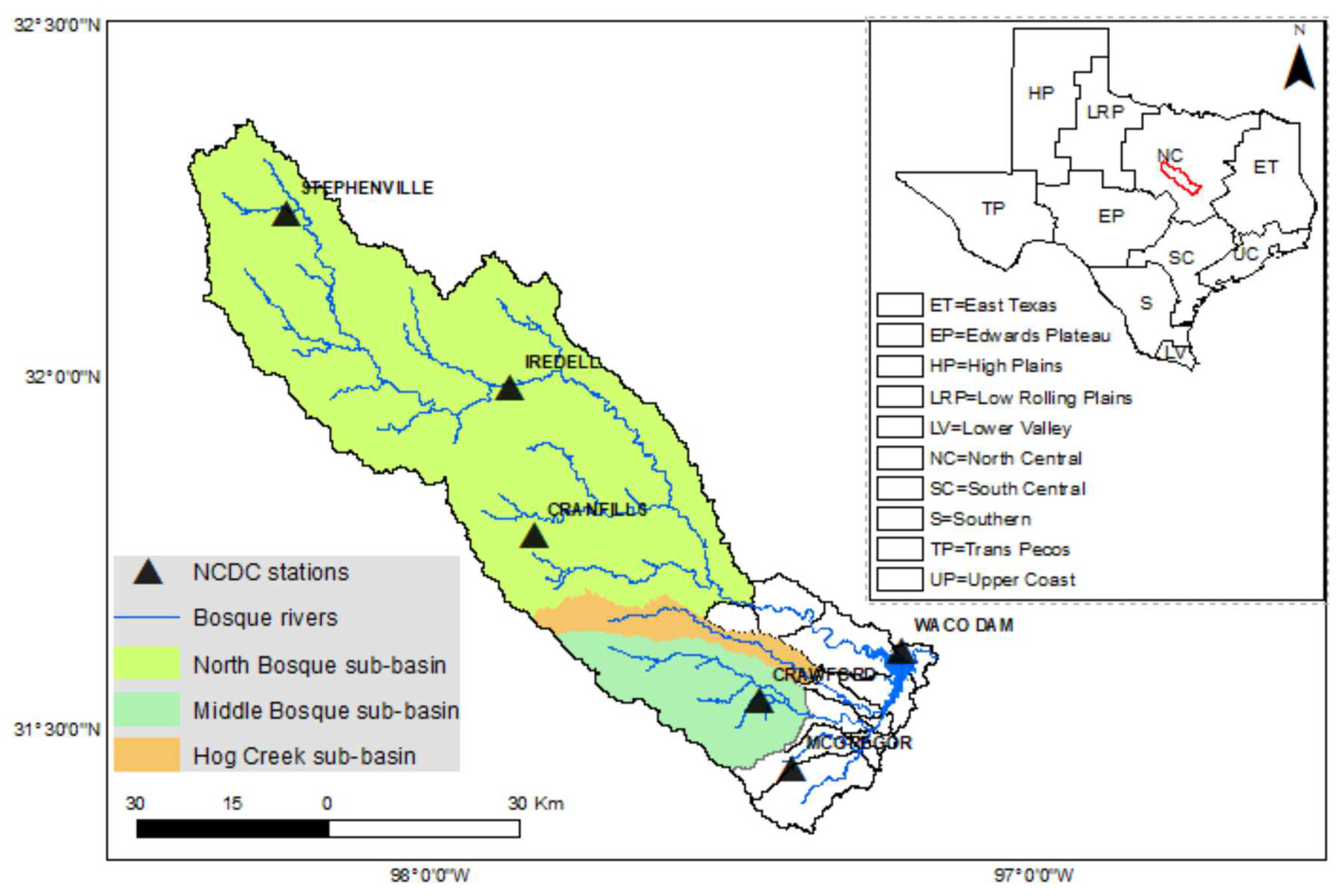
2.1. Study Area

The Bosque watershed is located in the Brazos River Basin, which covers seven out of ten climate zones of Texas. The watershed has an area of 4300 km2. The elevation in the watershed ranges from 111 m to 596 m (Figure 1). The Bosque River drains into Lake Waco and supplies drinking water for a large population of the Waco area. The Bosque watershed is covered by rangeland, woodland, forage fields, and dairy waste application fields. Dairy production and other agricultural enterprises include peanut, range-fed cattle, pecan, peach, and forage hay production as the dominant agricultural activities [42].
The Bosque watershed, located in the North-Central Texas climate division of Texas, is characterized by a warm temperate sub-humid climate. The average annual precipitation ranges from 737 to 838 mm, and the daily mean temperature ranges from 36 °F in January to 96 °F in July [43]. The environment of the Bosque watershed is characterized by high-intensity short-duration precipitation events and other precipitation extreme events that can cause large surface runoff [43,44]. Winter and fall precipitation are induced by continental polar fronts that produce low-intensity long-duration storms. In the spring and summer, most precipitation events produce high-intensity short-duration storms that can result in flooding in small watersheds.
Several rivers and streams, such as Hico, Valley Mills, and Clifton, contribute to the Bosque River. Storm-driven runoff is a primary hydrologic event and a source of water quality impairment in the North Bosque River [45]. Water pollution is the major water-related problem in the Bosque watershed. In 2000, this watershed was identified as an elevated concern for increased levels of nutrients entering the watershed from tributary watersheds; high levels of sediments, N, and P were identified [41].

2.2. Description of Gridded Precipitation Datasets

This study used in situ, gauge-based, satellite-based, and satellite-based gauge-corrected precipitation datasets: Global Historical Climatology Network (GHCN), Daymet, Parameter-elevation Regressions on Independent Slopes Model (PRISM), Integrated Multi-satellitE Retrievals for GPM (IMERG), Precipitation Estimation from Remotely Sensed Information using Artificial Neural Networks (PERSIANN), and Climate Hazards Group InfraRed Precipitation with Station data (CHIRPS). Station-based daily and monthly GHCN data are archived at the NOAA National Climate Data Center (NCDC). Thus, the NCDC refers to the GHCN data of the gauged stations. The descriptions of these datasets are included in Table 1.
For hydrologic modeling, ArcSWAT uses sub-basin level input rainfall data. For a particular sub-basin, it takes the rainfall data from the rain gauge closest to the centroid of that sub-basin; our model setup has 86 sub-basins. Rainfall data for these 86 sub-basin centroids were extracted from all the gridded data sets. Depending on the resolution of the gridded dataset and the size of the sub-basins, many of these sub-basins had the same rainfall inputs. Coarse resolution gridded products had a higher number of sub-basins with the same rainfall. In other words, finer resolution gridded data provided higher spatial variability in rainfall input data to drive the sub-basin scale hydrologic process in ArcSWAT. For rainfall comparison with the reference NCDC data, we used the extracted data for the grid.

2.2.1. Global Historical Climatology Network

GHCN is an integrated database of daily and monthly climate summaries collected from over 100,000 ground stations in 218 countries and territories across the globe [53]. The station’s dataset commonly included meteorological variables are: precipitation, minimum and maximum temperature, snowfall, and snow depth. Station data collected from numerous sources are merged and subjected to a common suite of quality assurance procedures to generate GHCN data.

2.2.2. Daymet

The Daymet dataset provides daily estimates of gridded (1 km × 1 km) solar radiation, maximum and minimum temperature, precipitation, snow water equivalent, and water vapor over the continental United States, Hawaii, and Puerto Rico. The Daymet dataset is generated using local regression algorithms to interpolate and extrapolate daily meteorological observations obtained from land surface metrological stations [47]. Daily observed weather data of maximum and minimum temperature and precipitation used to generate Daymet data are obtained from GHCN-Daily. Daymet uses the weighted linear regression-based approach to consider the effect(s) of elevation on climate and to generate the daily meteorological variables for a particular grid cell. Surrounding weather stations to each grid cell are selected and distance is weighted using a truncated Gaussian filter that considers the local station density [17].

2.2.3. Parameter-elevation Regressions on Independent Slopes Model (PRISM)

The PRISM dataset summarizes six essential climate parameters: precipitation, maximum and minimum temperature, dew point, and maximum and minimum vapor pressure. Station-level climate data collected from multiple sources are used with various modeling techniques to generate daily/monthly climate data from 1895 to the present. PRISM primarily combines Climatologically Aided Interpolation (CAI) and Radar Interpolation to generate daily climate summaries (PRISM Climate Group, 2019). The CAI method uses long-term average monthly climate as predictor grids to generate daily gridded data. Like Daymet, PRISM also uses a weighted linear regression approach with in situ station data and DEM to generate gridded climatic variables. However, in addition to elevation, PRISM explicitly accounts for environmental variables such as terrain-induced climate transitions, the effects of terrain as barriers, cold air drainage and inversions, and coastal effects [17].

2.2.4. Integrated Multi-satellitE Retrievals for GPM (IMERG)

The Integrated Multi-satellitE Retrievals for GPM (IMERG) algorithm uses information from GPM satellites to estimate precipitation over most of the earth’s surface. Precipitation estimates generated using passive microwave sensor data into the Goddard Profiling Algorithm (2017 version) are gridded and inter-calibrated to the GPM Combined Radar Radiometer to generate half-hourly precipitation fields at 0.1° resolution [54]. The latest IMERG dataset version 06 combines the early precipitation estimates collected during the TRMM (2000–2015), with more recent precipitation estimates generated from GPM satellites (2014–present). Three popular IMERG products were used in this study: Early, Late, and Final. The IMERG system runs twice to generate near real-time datasets, Early and Late, after ~4 h and 14 h of the observation time, respectively. The IMERG Final run uses observed monthly gauge data from the Global Precipitation Climatology Centre (GPCC) and the European Centre for Medium-Range Weather Forecasts (ECMWF) reanalysis data for final calibration [21].

2.2.5. Climate Hazards Group InfraRed Precipitation with Station Data (CHIRPS)

CHIRPS is a quasi-global (50°S–50°N, 180°E–180°W) precipitation dataset that provides daily and monthly precipitation estimates at 0.05° resolution from 1981 to near present [51]. CHIRPS uses thermal infrared data as a primary input along with passive microwave data and measured monthly gauge data for bias correction to generate the final product. This dataset combines three types of information—global climatology, satellite estimates, and in situ observations—calculating different time steps from 6-hourly to 3-monthly aggregates to generate several precipitation products [51,55]. Since it is blended with ground measurements, CHIRPS is perceived to be more efficient in representing the rainfall field [56].

2.2.6. Precipitation Estimation from Remotely Sensed Information Using Artificial Neural Networks (PERSIANN)

The Precipitation Estimation from Remotely Sensed Information using Artificial Neural Networks (PERSIANN) system is used to generate three datasets—PERSIANN (CHRS), PERSIANN-Cloud Computing System (CCS), and PERSIANN-Climate Data Records (CDR)—providing a range of spatio-temporal resolutions (Table 1). The PERSIANN system primarily uses infrared and visible data obtained from geostationary satellites [25]. PERISANN CHRS and PERSIANN-CCS use the satellite infrared imagery provided by the NOAA NCEP Climate Prediction Center. PERSIANN (CHRS) uses an Artificial Neural Network (ANN) model to develop a relationship between infrared (cloud) data and rainfall rates. PERSIANN-CCS segments the cloud into patches, clustered based on their temperature, texture, and geometry, to develop a relationship between cloud-top brightness temperature and rainfall for each cloud type [57].
PERSIANN-CDR uses an algorithm similar to CHRS. The main difference is that PERSIANN-CDR uses NCEP Stage IV hourly precipitation data instead of microwave data for ANN model training and bias correction [52]. The PERSIANN-CDR algorithm uses an additional bias correction step using monthly gridded (2.5°) precipitation data from the Global Precipitation Climatology Project (GPCP) [52]. The PERSIANN-CDR system uses NOAA NCEP GridSat-B1 infrared data to generate historical daily precipitation data.

2.3. Gridded Precipitation Datasets Performance Evaluation

The GHCN data of the gauged stations were acquired from the NCDC. Thus, NCDC data were used as a reference to evaluate the efficiency of gridded precipitation datasets. The output of gridded precipitation datasets was compared with the in situ NCDC data. This study used statistical metrics such as correlation, standard deviation, RMSE (root mean square error), NSE (Nash–Sutcliffe efficiency), KGE (Kling–Gupta efficiency), and PBIAS (percent bias) to evaluate the gridded daily, monthly, and annual precipitation datasets. The NSE [58] is a statistic used to evaluate the relative magnitude of the residual variance compared with the observed data variance. The KGE is the alternative and improved metric that combines NSE components (bias, correlation, and ratio of variances) in a more balanced way. In both NSE and KGE, values near 1 indicate strong model efficiency, while negative and positive values are viewed as bad and good model efficiency [59]. The PBIAS is a statistical metric that measures the average tendency of the simulated data whether it is larger or smaller than the observed data. A negative PBIAS value indicates the model’s overestimates, while a positive PBIAS value indicates the model’s underestimates of the observed values [60].
The Taylor diagram [61] was used to evaluate the ability of gridded precipitation datasets to capture in situ precipitation data. Correlation, RMSE, and standard deviation between in situ and gridded datasets were analyzed using the Taylor diagram. The cumulative distribution function (CDF) was also used to compare the distribution of precipitation events in the in situ and gridded precipitation datasets. In situ precipitation data during 2000–2019 at the selected GHCN weather stations (Figure 1) were compared (in and around the study watershed) against the gridded precipitation estimates for the corresponding grid containing the station.

2.4. Hydrologic Modeling

2.4.1. Description of the SWAT Model

SWAT is a robust hydrological model that was developed to estimate the effects of land use and management practices on water availability, sediment, and agricultural chemical yields over long periods in watersheds and river basins [62,63]. SWAT has been used to efficiently simulate the effect of climate change on water availability in different regions of the world [63,64,65,66]. The model uses the Soil Conservation Service (SCS) Curve Number method (USDA-SCS, 1972) to estimate surface runoff and the Penman–Monteith method to estimate potential evapotranspiration (PET).
In this study, SWAT was used to evaluate the effectiveness of gridded precipitation datasets in simulating the streamflow of the Bosque watershed. SWAT has previously been used to effectively simulate the streamflow and sediment load in the upper North Bosque watershed [42].

2.4.2. SWAT Model Calibration and Validation
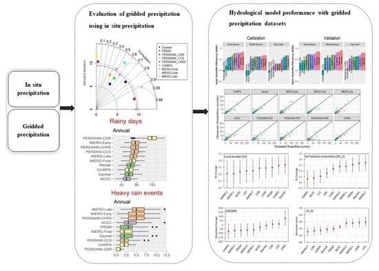
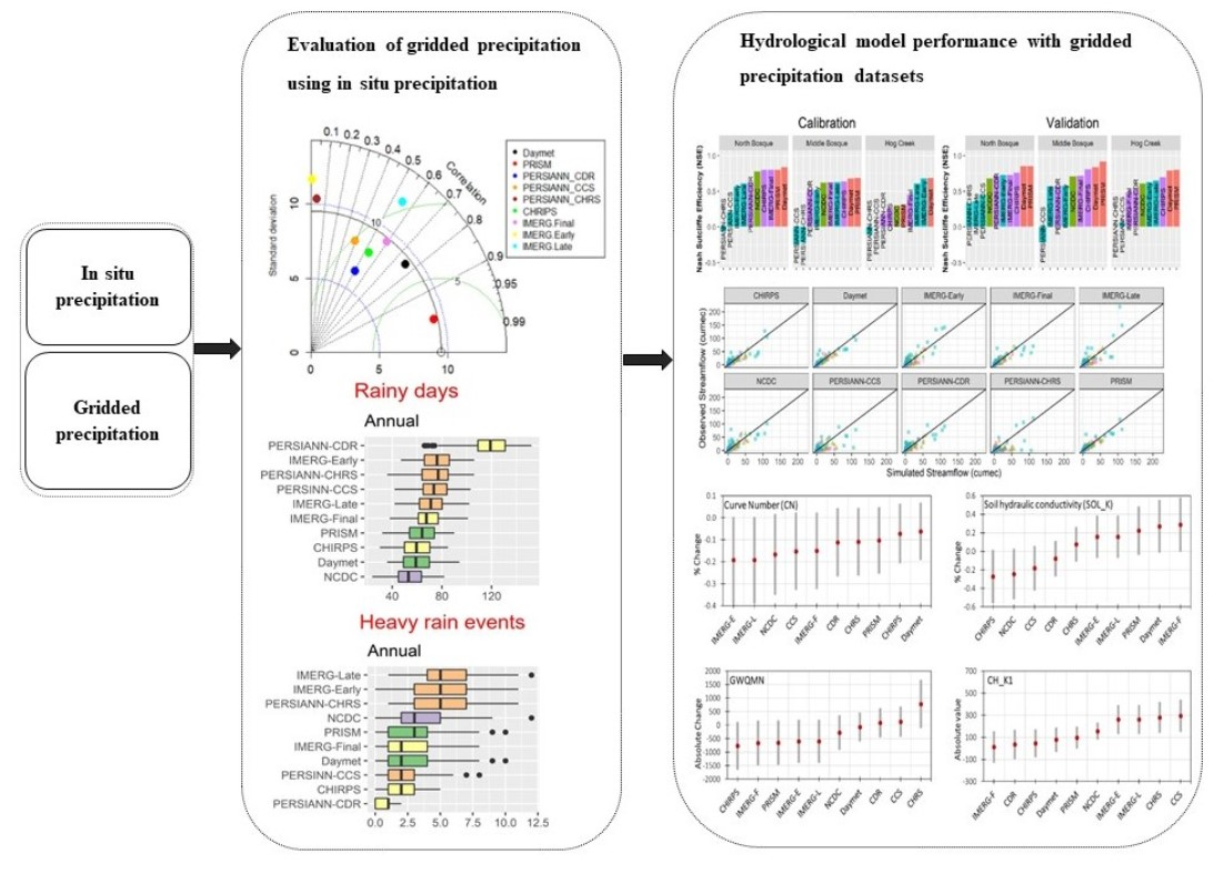
The SWAT model was calibrated and validated using in situ and gridded precipitation datasets at different gauge locations of the watershed (Figure 1). The SWAT model has numerous parameters which could affect the streamflow simulation. Thus, the most sensitive parameters of SWAT (parameters that have smaller p-value and larger t-stat) [67] were identified through a global sensitivity analysis in SWAT Calibration and Uncertainty Programs (SWAT-CUP) (Table 2). SWAT-CUP is an interface developed for SWAT and used to link the input/output, sensitivity analysis, calibration/validation, and uncertainty analysis of the SWAT model [67]. It intends to integrate calibration and validation with an uncertainty analysis in one user interface that further helps users compare observed and simulated results by creating graphs [68]. SWAT-CUP supports different optimization algorithms such as SUFI2, GLUE, and ParaSol [67]. Subsequently, the hydrological model was calibrated and validated using Sequential Uncertainty Fitting version 2 (SUFI2) SUFI-2 in SWAT-CUP [68]. SUFI is an optimization algorithm that estimates the uncertainty in model parameters, driving variables (e.g., precipitation), conceptual model, and observed data [69]. SUFI-2 measures uncertainties of parameters as ranges and is expressed as the 95% probability distributions calculated as the 2.5% and 97.5% levels of cumulative distribution [67,69]. SUFI-2 mainly involves defining an objective function, setting maximum and minimum values of parameters being optimized, sensitivity analysis, and assessing the uncertainties [69].
Calibration and validation were conducted for each gridded precipitation dataset and observational gauge station (NCDC) data. This means ten sets of precipitation data were used for calibrations and validations at each streamflow gauge of the Bosque watershed (Figure 1). The measured streamflow of 2002–2008 was used for model calibration, while the measured streamflow of 2014–2019 was used for model validation. Hydrological model efficiency in simulating the observed streamflow for each dataset was evaluated using KGE, NSE, and PBIAS, which are important goodness-of-fit evaluation criteria [60,67].
Furthermore, the uncertainty in the model simulation of streamflow was evaluated using the r-factor and the p-factor on the SUFI-2 algorithm. The p-factor is the percentage of the observed data bracketed within the 95PPU (95 Percent Prediction Uncertainty), whereas the r-factor measures the thickness of the uncertainty band. A p-factor of 1 and an r-factor of 0 indicate the exact fit of simulation with measurement [67].

3. Results

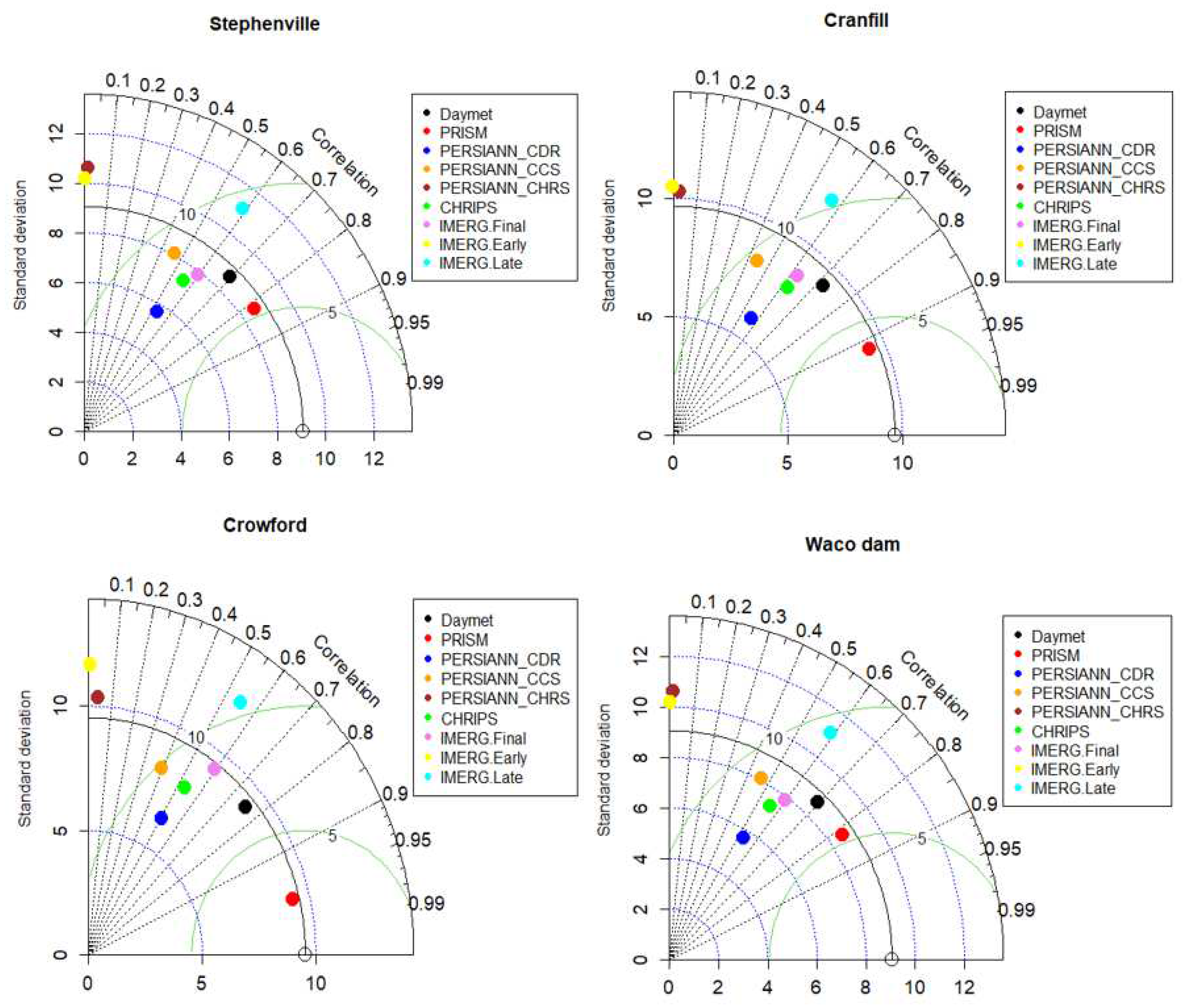
3.1. Comparison of Gridded Precipitation with In Situ Precipitation

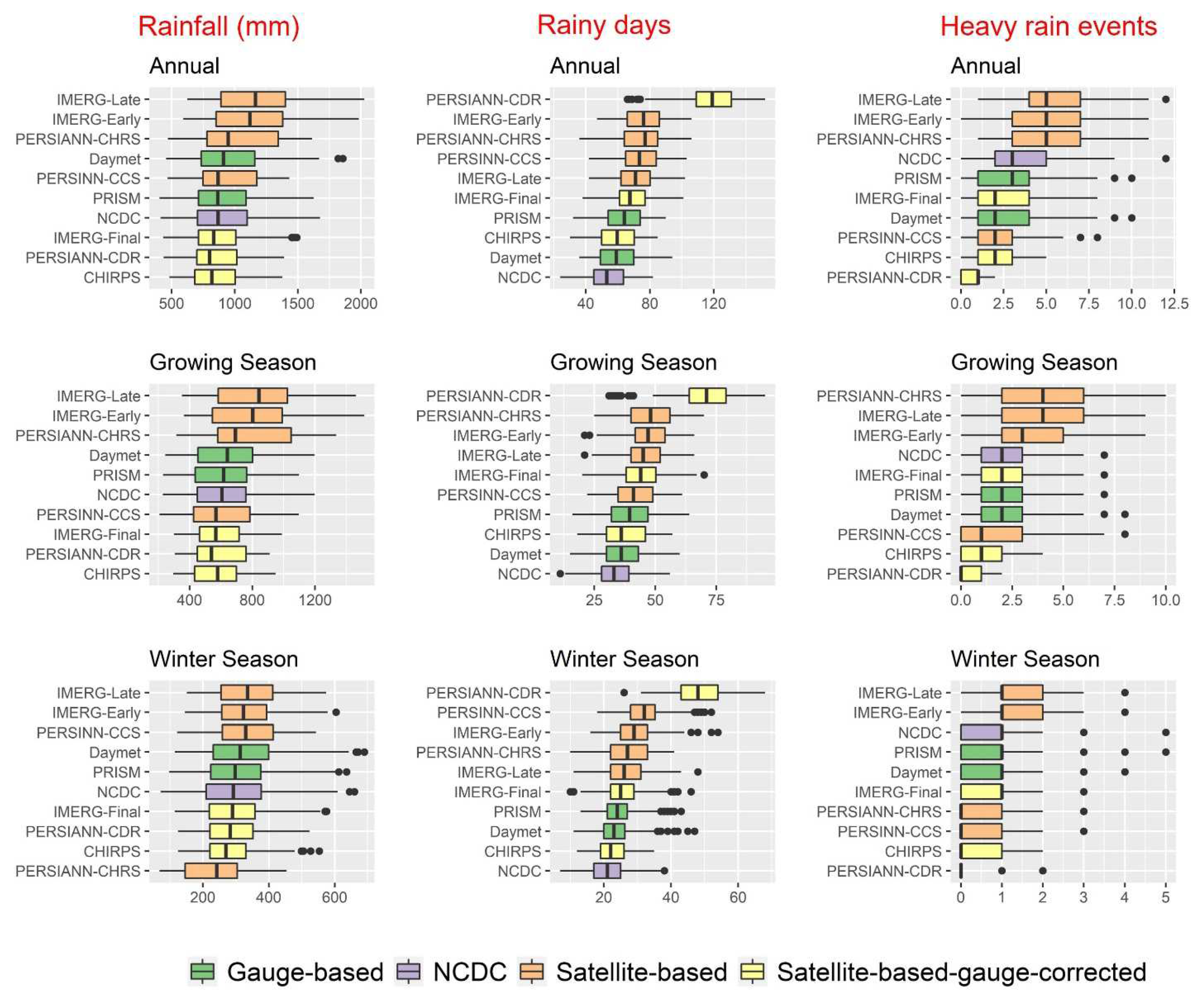
3.1.1. Daily Analysis

The Taylor diagrams show the evaluation of gridded precipitation datasets through the correlation, standard deviation, and RMSE between gridded precipitation datasets and the reference (in situ) precipitation data (Figure 2). The diagrams unfold the non-consistent ability of the gridded precipitation datasets in reproducing the in situ precipitation. Moreover, there is an apparent dissimilarity among the gridded datasets in a similar category. In most stations, the gauge-based gridded precipitation datasets (Daymet and PRISM) unveiled superior efficiency in correlation, RMSE, and standard deviation. For instance, Daymet and PRISM datasets have a better correlation with in situ precipitation than other precipitation products (Figure 2). In most stations, PRISM has a correlation of >0.8 with the in situ precipitation. The gauged-based datasets also disclose lower RMSE and standard deviation than other datasets in most stations. Remarkably, the PRISM dataset steadily achieves superior performance in RMSE and standard deviation in all stations (Figure 2). These high efficiencies are likely because the gauge-based datasets such as Daymet and PRISM are developed using precipitation observations from in situ stations.
However, satellite-based gridded datasets are weak in reproducing the in situ precipitation of the Bosque watershed (Figure 2). These gridded datasets have weak correlation, higher standard deviation, and RMSE from the in situ precipitation. Particularly, PERSIANN-CHRS, IMERG-Early, and IMERG-Late are characterized by weak correlation and high RMSE and standard deviation, confirming these datasets can provide considerable low-quality precipitation of the study watershed. PERSIANN-CCS is also under poor ability in correlation, RMSE, and standard deviation. Such low performance of satellite-based datasets may be attributed to biases stemming from cloud segmentation algorithms that classify clouds into patches or precipitation mapping methods for each classified cloud patch. This source of uncertainty is seldom found in gauge-based datasets.
The satellite-based gauge-corrected precipitation discloses moderate correlation, RMSE, and standard deviation (Figure 2). All of the gridded precipitation datasets in this group have correlation > 0.5 with the in situ dataset. IMERG-Late showed higher standard deviation and RMSE than other satellite-based gauge-corrected datasets. This designates a large difference between precipitation simulated by IMERG-Late and in situ precipitation. Thus, IMERG-Late and other datasets with higher standard deviation and RMSE, such as PERSIANN-CHRS and IMERG-Early, could overestimate or underestimate the in situ precipitation.
Daily time-series evaluations through KGE, NSE, and percent bias (PBIAS) unveiled the difference in the efficiency of gridded precipitation datasets (Figure 3). Based on the KGE, NSE, and PBIAS statistics, the increasing order of efficiency statistics were as follows: satellite-based, satellite-based gauge-corrected, and gauge-based datasets. However, in contrast to the other satellite-based gauge-corrected datasets, PERSIANN-CDR showed lower KGE (mean = 0.39) values than the satellite-based datasets such as IMERG-Late (mean = 0.47) and IMERG-Early (mean = 0.47). Lower KGE values for PERSIANN-CDR result from a low coefficient of variation (CV) of PERSIANN-CDR estimates compared with the CV of in situ station data. All the satellite-based products (IMERG-Late, IMERG-Early, PERSIANN-CHRS, and PERSIANN-CCS) revealed negative median NSE values, indicating a weaker performance than the mean predictor [59].
Using the Cumulative Distribution Function (CDF), the precipitation frequency and distribution in each dataset were compared to the observed gauged datasets (Figure S1). Some precipitation products such as Daymet, PRISM, CHIRPS, and PERSIANN-CHRS reproduce the CDF of the in situ precipitation. This indicates no strong systematic difference between groups of gridded precipitation datasets. Among the datasets, Daymet and PRISM PERSIANN (gauge-based), CHRS (satellite-based), and CHIRPS (satellite-based gauge-corrected) datasets well capture the distribution of in situ daily precipitation.
However, IMERG-Late, IMERG-Early, PERSIANN-CDR, and PERSIANN-CCS are inefficient in capturing the distribution of in situ precipitation at most of the gauge stations of the Bosque watershed. Unlike other gridded precipitation datasets, the distribution of IMERG-Late is characterized by a high proportion of extreme heavy precipitation values (>100 mm) in most areas of the watershed. In contrast, IMERG-Early, PERSIANN-CCS, and PERSIANN-CDR datasets show lower frequency distribution of high precipitation values. Particularly, IMERG-Early seamlessly underestimates the frequency distribution of high precipitation values. Concurrent to this study, the low performance of precipitation datasets in capturing the frequency of extreme precipitation was investigated by several researchers in different regions globally [70,71]. For instance, precipitation products such as CMORPH, PERSIANN, TMPA-RT, and TMPA-V6 revealed a weak ability to capture extreme precipitation in the central United States, Blue Nile Basin, and Yellow River Basin, respectively [70,71,72].

3.1.2. Monthly Analysis

Mean evaluation statistics of monthly precipitation indicated overall superior ability of gauge-based gridded datasets, PRISM (KGE = 0.92, NSE = 0.90, PBIAS = −0.9%) and Daymet (KGE = 0.91, NSE = 0.86, PBIAS = −4.7%) (Figure 4). On the other hand, PERSIANN-CHRS disclosed poor efficiency in terms of KGE (0.52), NSE (−0.30), and PBIAS (16.3) values. In general, satellite-based gauge-corrected datasets such as IMERG-Final, CHIRPS, and PERSIANN-CDR showed superior mean statistics (KGE = 0.75–0.82, NSE = 0.69–0.80, and PBIAS = 5.26 to 0.21) compared with the satellite-based products, which include IMERG-Late, IMERG-Early, PERSIANN-CCS, and PERSIANN-CHRS (KGE = 0.47 to 0.67, NSE = −0.30 to 0.32, and PBIAS = −27.69 to −3.37). Satellite-based products (IMERG-Early, IMERG-Late, and PERSIANN-CHRS) also overestimated annual and monthly precipitation ranging from 7 to 34%, depending on the station location. However, the satellite-based product (PERSIANN-CCS) showed a relatively low (mean PBIAS = −3.4%) overestimation bias that was comparable to the gauge-based (−0.9 to −4.7%) and satellite-based gauge-corrected (0.2 to 5.3%) datasets.
Gauge-based datasets (PRISM and Daymet) show low deviation in prediction accuracies between seasons (Figure 4). Satellite-based gauge-corrected datasets (IMERG-Final, CHIRPS and PERSIANN-CDR) showed slightly better mean statistics in the winter (November-May) season (KGE = 0.77 to 0.84, NSE = 0.70 to 0.82, PBAIS = −3.4 to 5.1%) compared with the growing (June-October) season (KGE = 0.73 to 0.80, NSE = 0.66 to 0.78, PBAIS=1.6 to 5.4%) (Figure 4). On the other hand, satellite-based products such as IMERG-Early, IMERG-Late, and PERSIANN-CHRS divulged better efficiency in the growing season in terms of NSE, KGE, and PBIAS values. PERSIANN-CHRS revealed low statistics, particularly in the winter season (KGE = 0.45, NSE = −0.65, and PBIAS = −23.6%). However, PERSIANN-CHRS has a better PBIAS value than IMERG-Late and IMERG-Early in the June-October season. In contrast to other satellite-based datasets, PERSIANN-CCS has better NSE and KGE values in the November-May season than the June-October season. We found that the PBIAS, PERSIANN-CCS overestimated (PBIAS = −19.3%) precipitation in the winter season, while it underestimated (PBIAS = 16%) during the growing season (Figure 4).

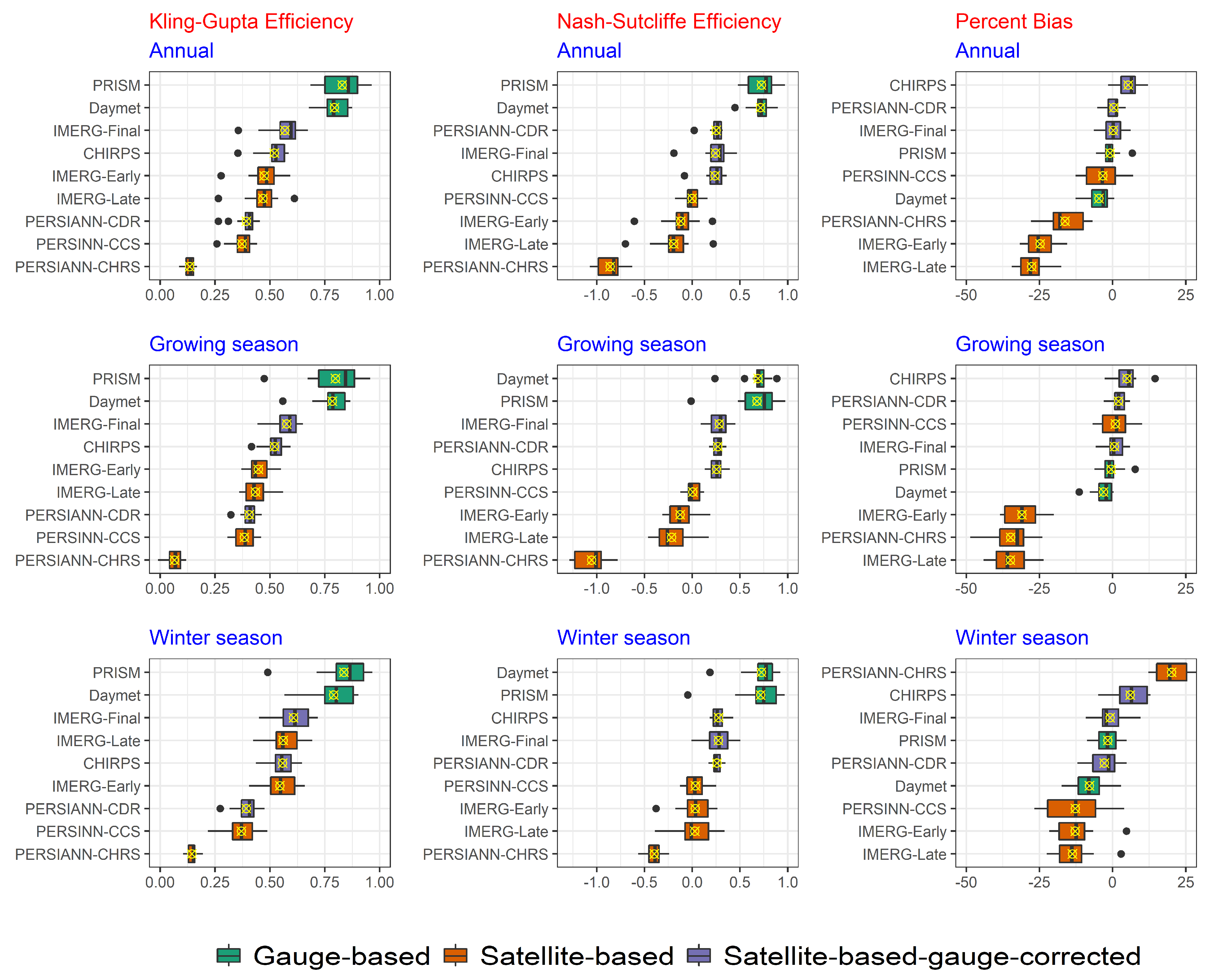
3.1.3. Annual and Seasonal Evaluation of Gridded Precipitation Datasets

At annual and seasonal scales, Daymet and PRISM datasets are superior in simulating the total precipitation, the precipitation days (>1 mm), and the heavy precipitation days than other precipitation products (Figure 5). However, gridded precipitation datasets from IMERG and PERSIANN groups struggle to simulate the mean and frequency of precipitation at annual and seasonal scales. For instance, the PERSIANN-CDR simulates a far higher number of wet days in the annual, growing, and winter seasons than the in situ gauges and other gridded datasets (Figure 5). However, the PERSIANN-CDR is characterized by fewer heavy precipitation events. This indicates that the precipitation in the PERSIANN-CDR is dominated by low-intensity and drizzle precipitation events. Satellite products such as IMERG-Early, IMERG-Late, and IMERG-CHRS are also characterized by a higher number of heavy precipitation events and precipitation days. In general, the systematic dissimilarity between the datasets is observed in simulating the mean and frequency of precipitation. The satellite-based datasets (IMERG-Late, IMERG-Early, and PERSIANN-CHRS) are characterized by a high frequency of heavy precipitation events during the annual, growing, and winter seasons.

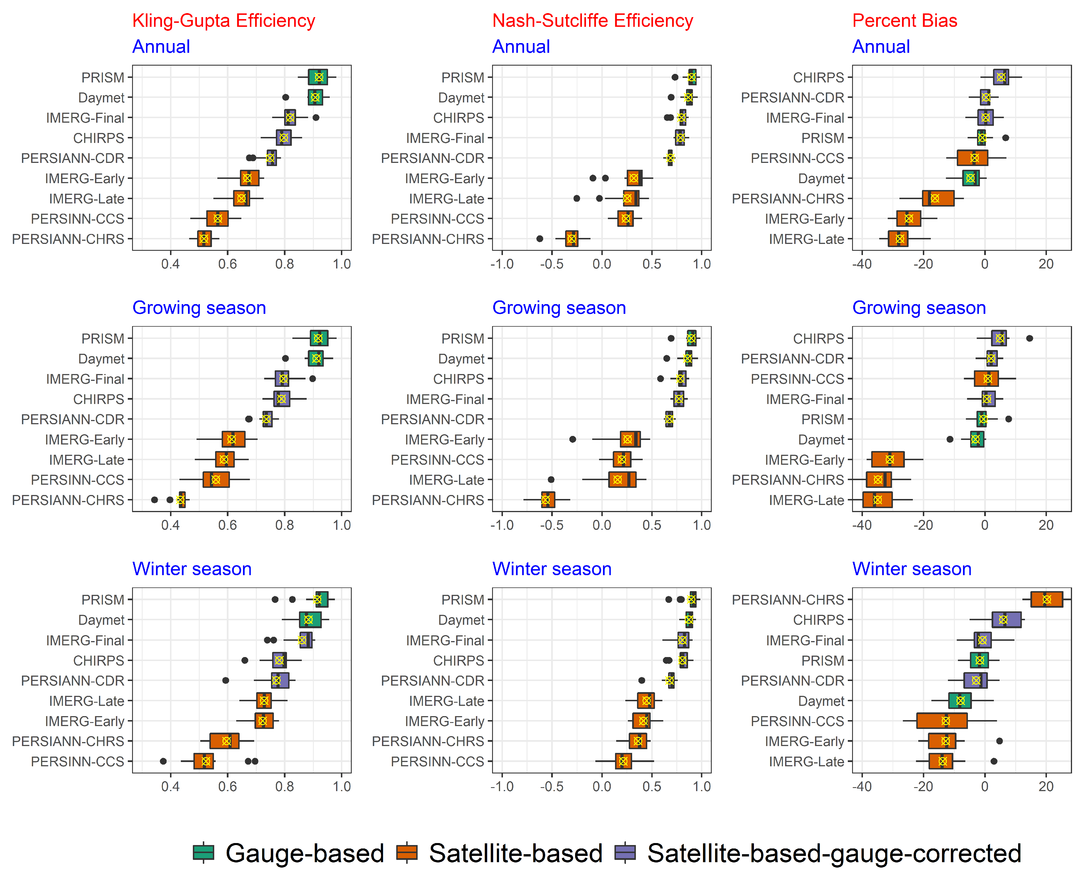
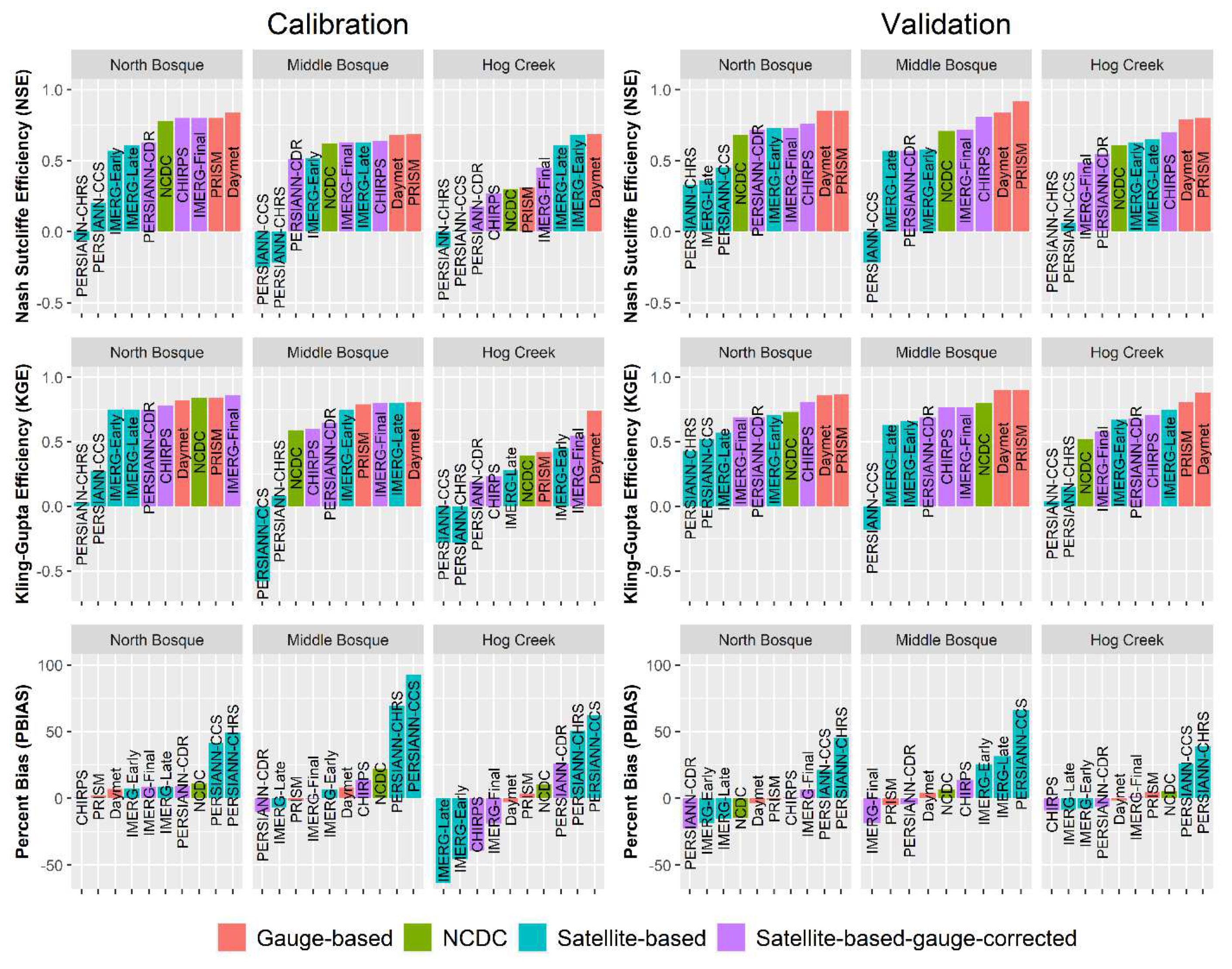
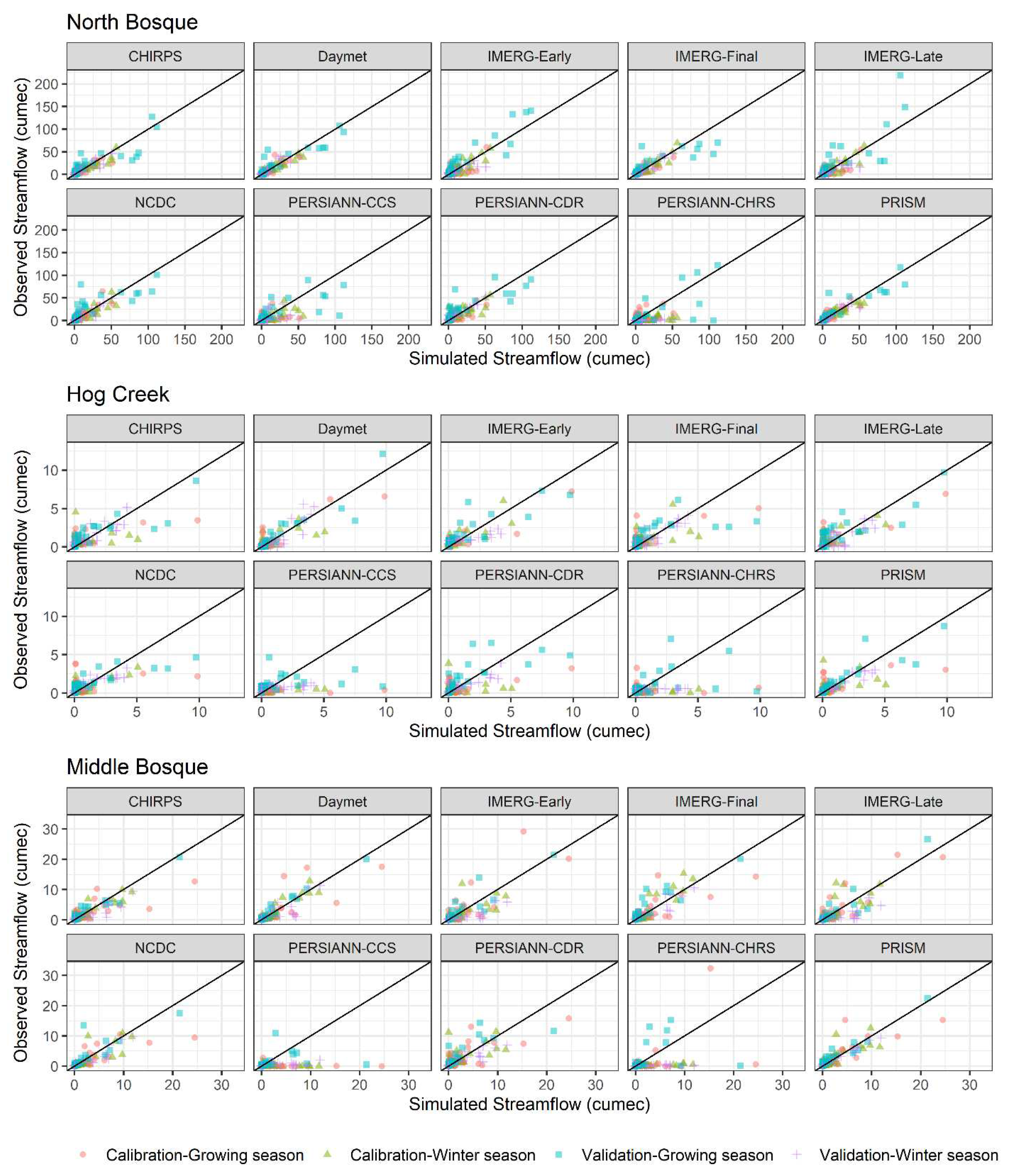
3.2. Hydrological Model Performance with Gridded Precipitation Datasets

Climate data such as precipitation are an important source of error that ascertain hydrological model strength [73,74,75]. This study also investigated the difference in hydrological model statistics for calibration and validation using different gridded precipitation datasets. The SWAT model simulation using in situ (NCDC), gauge-based (Daymet and PRISM), and satellite-based gauge-corrected (CHIRPS, IMERG-Final, and PERSIANN-CDR) precipitation data showed better NSE, KGE, and PBIAS during calibration and validation at the Bosque watershed (Figure 6). Furthermore, the SWAT model forced by Daymet and PRISM has better NSE and KGE during calibration and validation in the North Bosque, Middle Bosque, and Hog Creek sub-basins. This demonstrates that gridded precipitation datasets that show superior performance in capturing the mean and frequency of in situ precipitation better simulate the Bosque watershed’s streamflow. However, the SWAT model run by satellite-based datasets (PERSIANN-CHRS and PERSIANN-CCS) is characterized by the low efficiency of NSE, KGE, and PBIAS during calibration and validation. Analogously, the satellite-based datasets were far from simulating the mean and frequency of precipitation.
There is some coherence in the performance of gridded precipitation datasets during calibration and validation at the North Bosque, Middle Bosque, and Hog Creek gauges. Gridded datasets such as Daymet, PRISM, CHIRPS, and IMERG-Final consistently show superior efficiency at the North Bosque, Middle Bosque, and Hog Creek gauges. In contrast, gridded datasets such as PERSIANN-CHRS, PERSIANN-CCS, and PERSIANN-CHRS trigger low NSE, KGE, and PBIAS efficiency during calibration and validation at the North Bosque, Middle Bosque, and Hog Creek sub-basins.
Figure 7 representing a scatter plot of monthly streamflow, shows that gridded datasets can predict the streamflow of the Bosque watershed; however, the efficiency of gridded datasets in simulating streamflow is not similar. Concurrent with other metrics, the hydrological model, which uses precipitation data of Daymet, PRISM, CHIRPS, and IMERG-Final, unfolds a better correlation with observed streamflow. Particularly, model simulation using Daymet precipitation showed superior efficiency, even higher than the model driven by the in situ precipitation. However, the model simulation using IMERG-Late, PERSIANN-CHRS, and PERSIANN-CCS showed weak correlation with the observed streamflow.
The performance of gridded precipitation datasets in simulating observed streamflow is different at different sub-basins of the Bosque watershed. The hydrological model, which uses the precipitation of in situ (NCDC), Daymet, PRISM, CHIRPS, IMERG-Early, IMERG-Final, and PERSIANN-CDR, has a better correlation with the observed streamflow in the North Bosque sub-basin (Figure 7). Conversely, the hydrological model driven by PERSIANN-CDR, PERSIANN-CHRS, PERSIANN-CCS, PRISM, IMERG-Final, and IMERG-Early disclosed a lower association with the observed streamflow in the Hog Creek sub-basin than other sub-basins (Figure 7). This may be attributed to the difference in land use, area, and soil hydraulic characteristics between the sub-basins. In the Hog Creek sub-basin, the hydrological model forced by the Daymet precipitation has a relatively better association with observed streamflow than other datasets.
Another difference is the performance of gridded datasets among seasons. The hydrological model calibrated during the growing season and used in situ precipitation, CHIRPS, Daymet, PERSIANN-CCS, PERSIAN-CHRS, and IMERG-Early had a lower correlation with observed streamflow in the Middle Bosque sub-basin. On the other hand, the hydrological model validated during the winter season and used the precipitation of Daymet, CHIRPS, IMERG-Final, IMERG-Early, IMERG-Late, and PRISM showed a better correlation with observed streamflow in the Hog Creek sub-basin (Figure 7).

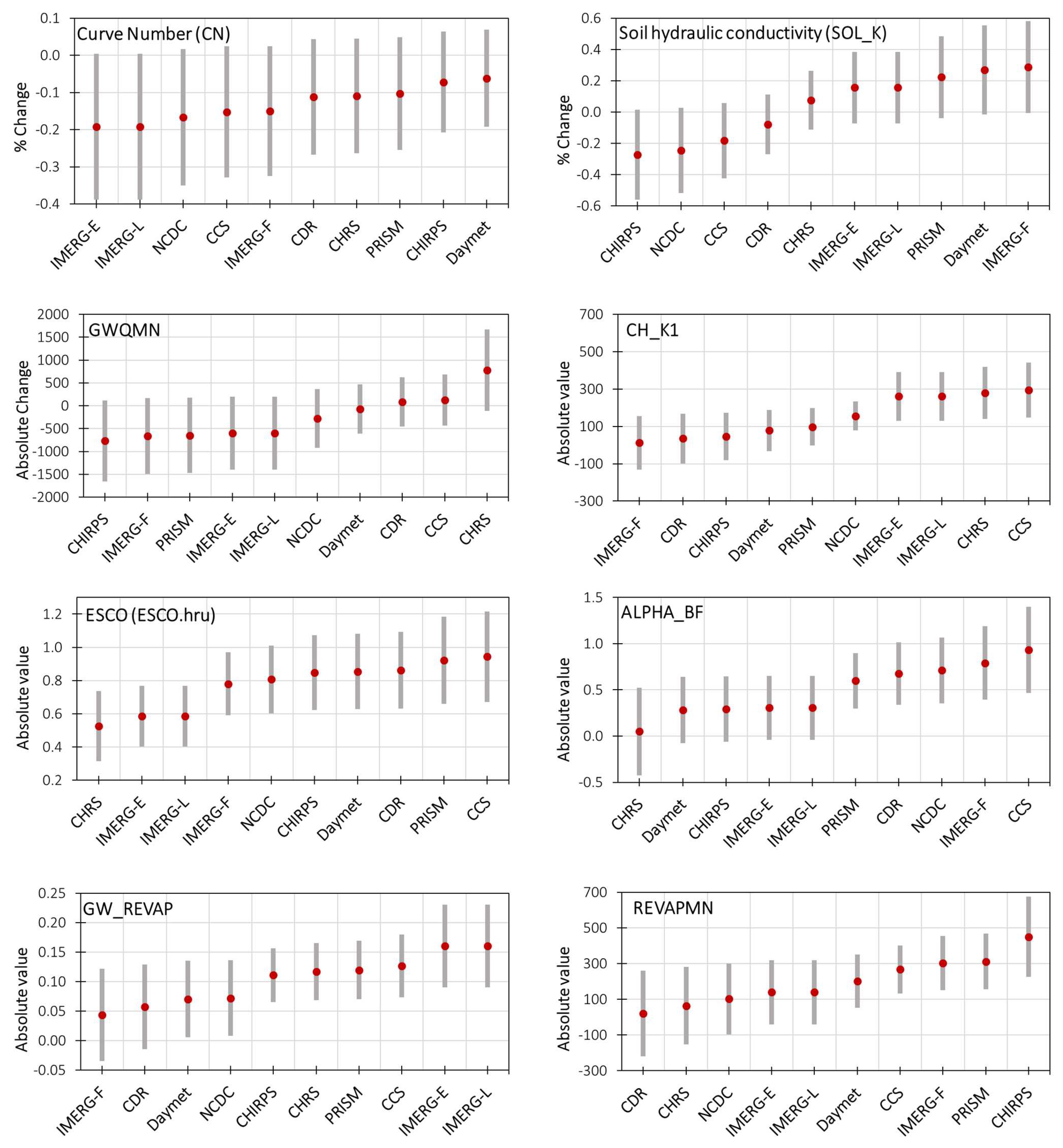
3.3. Uncertainties Due to Precipitation Data

Figure 8 presents the SWAT-CUP suggested optimum model input parameter ranges and best parameter values under different gridded precipitation datasets. The suggested range of optimum parameters designates the uncertainty largely stemming from input data (precipitation). Among the model input parameters, the Curve Number (CN) showed a large uncertainty band (Figure 8). The relative change in CN values ranges from −0.4 to 0.0 in the IMERG-Early and IMERG-Late datasets, while it ranges from −0.2 to 0.06 in the Daymet data. The soil hydraulic conductivity (SOL_K) and GWQMN parameters also show a large range of uncertainty. The relative change in SOL_K values is in the order of 0.6 to 0.0 in the CHIRPS dataset, while the relative change in SOL_K values is in the range of 0.0 to 0.6 in the IMERG-Final. The absolute value of GWQMN is between −1500 to 0 in the CHIRPS dataset and 0 to 1500 in the PERSIANN-CHRS dataset. The stream channel-related parameter, i.e., CH-K (effective channel hydraulic conductivity), illustrates a low uncertainty band during the calibration and validation of the hydrological model run by gridded precipitation datasets (Figure 8).
The SWAT model calibrated and validated using PERSIANN-CCS, PERSIANN-CHRS, CHIRPS, IMERG-Final, and IMERG-Early unveiled a higher increase or higher decrease in most of the SWAT parameters used for calibration. This demonstrates that such precipitation datasets can produce relatively higher changes in SWAT parameter values and can cause higher uncertainty in hydrological modeling.
Table 3 presents the uncertainties during calibration and validation of the hydrological model run by different gridded precipitation products at different sub-basins of the Bosque watershed. The hydrological model revealed a different level of p-factor and r-factor at different sub-basins of the watershed. In the North Bosque sub-basin of the watershed, the hydrological model calibrated using gridded precipitation datasets produces the recommended p-factor value (>0.7) [67]. The PERSIANN-CHRS dataset could not achieve a reasonable p-factor during calibration in the North Bosque sub-basin (Table 3). However, the hydrological model calibrated using most of the gridded datasets could not achieve the recommended r-factor value (<1.5) [67] in the North Bosque sub-basin. Only PERSIANN-CDR and CHIRPS datasets provided a reasonable r-factor in this sub-basin (Table 3). The hydrological model simulated using all gridded precipitation datasets during validation presented high p-factor values. Similarly, validation of the model under most gridded precipitation datasets also attained recommended r-factor values in the North Bosque watershed. The calibration and validation of the hydrological model run by gridded precipitation datasets showed lower p-factor and r-factor in the Middle Bosque and Hog creek sub-basins than in the North Bosque sub-basin. In these sub-basins, no recommended r-factor was achieved during calibration of the hydrological model driven by any gridded precipitation.
From the total 2000 simulations, the number of simulations with NSE > 0.5 during calibration and validation also showed a difference among the sub-basin (Table 3). The calibration and validation in the North Bosque sub-basin revealed a higher number of such simulations with NSE > 0.5 (Table 3). In the Hog Creek and Middle Bosque sub-basins of the Bosque watershed, a lower number of simulations achieved NSE > 0.5. In the Hog Creek sub-basin, the model was calibrated through PRISM’s input; PERSIANN-CHRS, PERSIANN-CDR, PERSIANN-CCS, CHIRPS, and NCDC did not achieve NSE > 0.5. In the Middle Bosque sub-basin, the hydrological model calibrated and validated using PERSIANN-CHRS and PERSIANN-CCS did not achieve NSE > 0.5. The SWAT model calibrated and validated by most gridded datasets showed low efficiency in achieving the recommended r-factor. Particularly, SWAT simulations run by PERSIANN-CHRS and PERSIANN-CCS steadily revealed low p-factor and r-factor values in the Hog Creek and Middle Bosque sub-basins.

4. Discussion

This study evaluated the performance of gridded precipitation datasets in reproducing the in situ precipitation and simulating observed streamflow of the Bosque watershed from 2000 to 2019. The results revealed discernable capability among different groups of gridded precipitation datasets in estimating daily, monthly, seasonal, and annual precipitation. The gauge-based products such as Daymet and PRISM showed superior performance in most metrics used for evaluation than other datasets. The Daymet and PRISM showed higher NSE and KGE (≥0.7 to 0.92) with the in situ precipitation at daily and monthly scales. These datasets also better captured the frequency of wet days and heavy precipitation events. This is because Daymet and PRISM use observed station data obtained from GHCN-Daily to develop spatially continuous gridded precipitation datasets. These datasets apply regression techniques such as linear regression and weighted linear regression to convert station-based (point) data into continuous gridded datasets [17]. Thus, the main source of uncertainty in these datasets could be from the interpolation techniques. In fact, the reliability of these datasets is highly dependent on the quality of observed data. The importance of these data sources can also be hindered where the density of observing gauge stations is sparse on mountainous, desert, and ocean surfaces with no gauge stations.
Satellite-based datasets such as IMERG (Early and Late) and PERSIANN groups had relatively low performance in most metrics. These datasets had low correlation, NSE, and KGE (<0.5 in most cases) with the in situ precipitation at daily, monthly, and annual scales. However, satellite-based datasets were found effective in simulating precipitation and hydrology in other regions of the USA [18,25,50,72,76]. The low efficiency of satellite-based datasets could be attributed to the biases in cloud parametrization and satellite sensors taking the image of the cloud over the Texas region by TRMM and GPM. The error in the image of satellite sensors of TRMM and GPM may also trigger a multiplicative error on the estimated precipitation that further limit such datasets from effectively representing precipitation of the region. Besides, the biases in satellite-based precipitation may be attributed to the limitations of satellites to capture the climate of Texas driven by the eastern tropical Pacific and tropical trade winds and characterized by highly variable moisture conditions [44,77]. It is worthwhile to disentangle the source of bias and the relative contribution of image taking and retrieval algorithms in contributing biases of satellite-based datasets in the Bosque watershed and the Texas region.
The PERSIANN products, particularly PERSIANN-CHRS and PERSIANN- CCS satellite-based products, were also found less reliable in estimating precipitation. The PERSIANN-CHRS and PERSIANN- CCS datasets use infrared imagery to measure cloud-top temperature and precipitation [57]; this means no direct measurement of precipitation-related events occurring at a lower altitude. Such techniques of image taking can be a source of uncertainty. The use of satellites and sensors to detect cloud water, water vapor, and long-wave radiations are improvements for better data collection from the earth’s surface and the lower atmosphere. Moreover, the PERSIANN system applies the Artificial Neural Networks (ANNs) technique to develop an association between cloud-top brightness temperature and rainfall for each cloud type [57]. The retrieval technique, which intends to associate the pixel brightness temperature rate using histogram matching and exponential regression, could also be a potential source of biases in the PERSIANN-CCS.
The satellite-based gauged-corrected datasets performed better in capturing in situ precipitation than the satellite-based products. For instance, CHIRPS showed good accuracies in correlation, NSE, and KGE and better captured the cumulative distribution of in situ precipitation. The gauge observations used by CHIRPS for the bias correction of satellite precipitation [51] may result in a better simulation of precipitation by CHIRPS. The IMERG-Final also showed better efficiency of correlation, NSE, and KGE than satellite-based products. However, IMERG-Final was characterized by overestimating precipitation and high frequency of heavy precipitation events in the distribution function than other datasets. Thus, the overestimation of IMERG-Final could emerge from the datasets used for bias correction or the multiplicative effect from the raw satellite data and the data used for bias correction. For instance, in the IMERG-Final, uncertainty may arise from the Global Precipitation Climatology Centre and European Centre for Medium-Range Weather Forecasts Reanalysis, which were used for calibration [21], or the multiplicative effect of errors from IMERG and the data used for calibration.
The hydrological model calibrated and validated through gridded precipitation datasets revealed a range of effectiveness in reproducing the observed streamflow at the gauge location of the Bosque watershed. Generally, input data error is not the only source of uncertainty; rather, hydrological model parameters and model conceptualization can also be an important source of uncertainty that can reduce the hydrological model’s efficiency [73,74,75]. Corresponding with the ability to capture in situ precipitation, the SWAT model calibrated and validated with gauged-based datasets such as Daymet and PRISM, and satellite-based gauge-corrected models such as CHIRPS and IMERG-Final have better accuracy in most metrics. However, hydrological models run by PERSIANN group datasets revealed poor efficiency in reproducing observed streamflow during calibration and validation. This indicates that input data error from gridded precipitation datasets is a significant source of uncertainty in the hydrological modeling of the Bosque watershed.

5. Conclusions

This study evaluated two gauge-based, four satellite-based, and three satellite-based gauge-corrected gridded precipitation products using different mean and distribution-based metrics. The results showed relative differences in the performance of the gridded precipitation datasets in capturing the in situ gauge precipitation and simulating streamflow of the Bosque watershed in Texas. Gauge-based precipitation products, Daymet and PRISM, showed the best performance reproducing the in situ precipitation. The Daymet and PRISM revealed a NSE of ≥0.7 and ≥0.86 with the in situ precipitation at daily and monthly scales, respectively. These gauge-based precipitation datasets are also better in capturing the frequency of wet days and heavy precipitation events than other datasets. The hydrological model simulated using Daymet and PRISM outputs showed NSE and KGE of ≥0.75 at most of the gauges used for calibration and validation. Next to gauge-based precipitation products, satellite-based gauge-corrected products such as CHIRPS and IMERG-Final unveiled better performances. Corresponding to these results, the hydrological model (SWAT) calibrated and validated using gauge-based and satellite-based gauge-corrected products revealed better NSE and KGE efficiency (≥0.7 in most cases) in the Bosque watershed. Satellite-based datasets such as PERSIANN-CCS and PERSIANN-CCS showed weak NSE and KGE efficiency (<0.5) in reproducing precipitation and observed streamflow during SWAT calibration and validation.
Most essentially, this study has estimated the uncertainties in SWAT parameters under gridded precipitation datasets. The SWAT parameters which were used for calibration and validation showed different degrees of uncertainty as a response to gridded precipitation datasets. When the SWAT model was forced by satellite-based precipitation, most calibration and validation parameters showed a large band of uncertainty, while the SWAT parameters showed a narrow band of uncertainty when the gauged-based precipitation datasets were used. Parameter uncertainty analysis also showed the variation of parameter values when using different gridded datasets. For instance, the calibrated Curve Number (CN) value is −0.2 when using satellite-based datasets, while it is greater than −0.1 when using gauge-based datasets. Overall, we conclude that most gridded datasets can provide reliable precipitation information for hydrologic modeling at monthly time-scale analyses, but the gauge-based datasets showed superior performance in simulating hydrology and parameter uncertainty analysis.
Even though gridded precipitation datasets such as the gauged-based and satellite-based gauge-corrected datasets reasonably capture in situ precipitation and streamflow, it is worthwhile to work to continuously improve the quality of these datasets in the years to come. This study suggests extensive efforts are needed to develop precipitation datasets that can effectively capture the mean, frequency, and intensity of the in situ precipitation, especially at daily or sub-daily time scales. Therefore, satellite observations, retrieval algorithms to convert satellite data to precipitation, and better interpolation techniques are nontrivial for a better understanding of historical climate. Furthermore, continuous improvement in gridded precipitation datasets may also increase the effectiveness of hydrological model simulations.
The results of this study could represent other regions of the USA with similar climates and topography. Particularly, the findings represent North-Central Texas, characterized by plain topography and climate condition characterized by high variability and driven by the tropical storms originating from the eastern tropical Pacific [77]. The calibrated and validated SWAT parameters can be used in other watersheds of North-Central Texas, which have similar land use, topography, and climate conditions following the parameter transfer approach [78,79]. However, the findings of the study may not generalize other regions of the world characterized by scarce in situ observations, diverse physiography, and the climate condition controlled by local topography and large-scale climate drivers.

Supplementary Materials

The following are available online at https://www.mdpi.com/article/10.3390/rs14163860/s1, Figure S1: Cumulative Distribution Function compares daily in situ precipitation with gridded precipitation datasets in the upper, middle, and downstream courses of the Bosque watershed.

Author Contributions

R.L.R. contributed to the design, discussion, and write-up of the manuscript; R.P.S. contributed to the data preparation, methodology, and data analysis of the manuscript; G.W.T. was involved in the data analysis, discussion, and write-up of the manuscript. All authors have read and agreed to the published version of the manuscript.

Funding

This work was funded by the United States Department of Agriculture (USDA) National Institute of Food and Agriculture (NIFA), Capacity Building Grants (CBG) 1018084.

Data Availability Statement

The data will be available on request from the corresponding author.

Acknowledgments

We thank Eric Risch for his time to edit this paper. We also thank graduate student Esther Kayode for her help in the literature review.

Conflicts of Interest

The authors declare no conflict of interest.

References

  1. Bajracharya, A.R.; Bajracharya, S.R.; Shrestha, A.B.; Maharjan, S.B. Climate change impact assessment on the hydrological regime of the Kaligandaki Basin, Nepal. Sci. Total Environ. 2018, 625, 837–848. [Google Scholar] [CrossRef] [PubMed]
  2. Maraun, D.; Rust, H.W.; Osborn, T.J. Synoptic airflow and UK daily precipitation extremes. Extremes 2010, 13, 133–153. [Google Scholar] [CrossRef]
  3. Jódar, J.; Carpintero, E.; Martos-Rosillo, S.; Ruiz-Constán, A.; Marín-Lechado, C.; Cabrera-Arrabal, J.A.; Navarrete-Mazariegos, E.; González-Ramón, A.; Lambán, L.; Herrera, C.; et al. Combination of lumped hydrological and remote-sensing models to evaluate water resources in a semi-arid high altitude ungauged watershed of Sierra Nevada (Southern Spain). Sci. Total Environ. 2018, 625, 285–300. [Google Scholar] [CrossRef]
  4. Abatzoglou, J.T. Development of gridded surface meteorological data for ecological applications and modelling. Int. J. Climatol. 2013, 33, 121–131. [Google Scholar] [CrossRef]
  5. Raimonet, M.; Oudin, L.; Thieu, V.; Silvestre, M.; Vautard, R.; Rabouille, C.; Le Moigne, P. Evaluation of gridded meteorological datasets for hydrological modeling. J. Hydrometeorol. 2017, 18, 3027–3041. [Google Scholar] [CrossRef]
  6. Sperna Weiland, F.C.; Vrugt, J.A.; van Beek, R.L.P.H.; Weerts, A.H.; Bierkens, M.F.P. Significant uncertainty in global scale hydrological modeling from precipitation data errors. J. Hydrol. 2015, 529, 1095–1115. [Google Scholar] [CrossRef] [Green Version]
  7. Strauch, M.; Bernhofer, C.; Koide, S.; Volk, M.; Lorz, C.; Makeschin, F. Using precipitation data ensemble for uncertainty analysis in SWAT streamflow simulation. J. Hydrol. 2012, 414–415, 413–424. [Google Scholar] [CrossRef]
  8. Schamm, K.; Ziese, M.; Becker, A.; Finger, P.; Meyer-Christoffer, A.; Schneider, U.; Schröder, M.; Stender, P. Global gridded precipitation over land: A description of the new GPCC First Guess Daily product. Earth Syst. Sci. Data 2014, 6, 49–60. [Google Scholar] [CrossRef] [Green Version]
  9. Harris, I.; Osborn, T.J.; Jones, P.; Lister, D. Version 4 of the CRU TS monthly high-resolution gridded multivariate climate dataset. Sci. Data 2020, 7, 109. [Google Scholar] [CrossRef] [Green Version]
  10. Chen, C.T.; Knutson, T. On the verification and comparison of extreme rainfall indices from climate models. J. Clim. 2008, 21, 1605–1621. [Google Scholar] [CrossRef]
  11. Javanmard, S.; Yatagai, A.; Nodzu, M.I.; Bodaghjamali, J.; Kawamoto, H. Comparing high-resolution gridded precipitation data with satellite rainfall estimates of TRMM-3B42 over Iran. Adv. Geosci. 2010, 25, 119–125. [Google Scholar] [CrossRef] [Green Version]
  12. Jing, X.; Geerts, B.; Wang, Y.; Liu, C. Evaluating seasonal orographic precipitation in the interior western United States using gauge data, gridded precipitation estimates, and a regional climate simulation. J. Hydrometeorol. 2017, 18, 2541–2558. [Google Scholar] [CrossRef]
  13. Tang, X.; Zhang, J.; Gao, C.; Ruben, G.B.; Wang, G. Assessing the uncertainties of four precipitation products for SWAT modeling in Mekong River Basin. Remote Sens. 2019, 11, 304. [Google Scholar] [CrossRef] [Green Version]
  14. Sun, Q.; Miao, C.; Duan, Q.; Ashouri, H.; Sorooshian, S.; Hsu, K.L. A Review of Global Precipitation Data Sets: Data Sources, Estimation, and Intercomparisons. Rev. Geophys. 2018, 56, 79–107. [Google Scholar] [CrossRef] [Green Version]
  15. Tang, L.; Zhang, J.; Simpson, M.; Arthur, A.; Grams, H.; Wang, Y.; Langston, C. Updates on the radar data quality control in the MRMS quantitative precipitation estimation system. J. Atmos. Ocean Technol. 2020, 37, 1521–1537. [Google Scholar] [CrossRef]
  16. Behnke, R.; Vavrus, S.; Allstadt, A.; Albright, T.; Thogmartin, W.E.; Radeloff, V.C. Evaluation of downscaled, gridded climate data for the conterminous United States. Ecol. Appl. 2016, 26, 1338–1351. [Google Scholar] [CrossRef]
  17. Daly, C. Guidelines for assessing the suitability of spatial climate data sets. Int. J. Climatol. 2006, 26, 707–721. [Google Scholar] [CrossRef]
  18. Beck, H.E.; Pan, M.; Roy, T.; Weedon, G.P.; Pappenberger, F.; Van Dijk, A.I.J.M.; Huffman, G.J.; Adler, R.F.; Wood, E.F. Daily evaluation of 26 precipitation datasets using Stage-IV gauge-radar data for the CONUS. Hydrol. Earth Syst. Sci. 2019, 23, 207–224. [Google Scholar] [CrossRef] [Green Version]
  19. Karbalaee, N.; Hsu, K.; Sorooshian, S.; Braithwaite, D. Bias adjustment of infrared-based rainfall estimation using Passive Microwave satellite rainfall data. J. Geophys. Res. Atmos. 2017, 122, 3859–3876. [Google Scholar] [CrossRef] [Green Version]
  20. Sorooshian, S.; Hsu, K.-L.; Coppola, E.; Tomassetti, B.; Verdecchia, M.; Visconti, G. Hydrological Modelling and the Water Cycle: Coupling the Atmospheric and Hydrological Models; Springer: Berlin/Heidelberg, Germany, 2009. [Google Scholar]
  21. Huffman, G.J.; Stocker, E.F.; Bolvin, D.T.; Nelkin, E.J.; Tan, J. GPM IMERG Final Precipitation L3 1 Day 0.1 Degree × 0.1 Degree V06 (GPM_3IMERGDF) at GES DISC. 2019. Available online: http://www.10.5067/GPM/IMERGDF/DAY/06 (accessed on 4 July 2022).
  22. Huffman, G.J.; Bolvin, D.T.; Nelkin, E.J.; Wolff, D.B.; Adler, R.F.; Gu, G.; Hong, Y.; Bowman, K.P.; Stocker, E.F. The TRMM Multisatellite Precipitation Analysis (TMPA): Quasi-global, multiyear, combined-sensor precipitation estimates at fine scales. J. Hydrometeorol. 2007, 8, 38–55. [Google Scholar] [CrossRef]
  23. Xie, P.; Joyce, R.; Wu, S.; Yoo, S.H.; Yarosh, Y.; Sun, F.; Lin, R. Reprocessed, bias-corrected CMORPH global high-resolution precipitation estimates from 1998. J. Hydrometeorol. 2017, 18, 1617–1641. [Google Scholar] [CrossRef]
  24. Aonashi, K.; Awaka, J.; Hirose, M.; Kozu, T.; Kubota, T.; Liu, G.; Shige, S.; Kida, S.; Seto, S.; Takahashi, N.; et al. Gsmap passive microwave precipitation retrieval algorithm: Algorithm description and validation. J. Meteorol. Soc. Jpn. Ser. II 2009, 87, 119–136. [Google Scholar] [CrossRef] [Green Version]
  25. Nguyen, P.; Ombadi, M.; Sorooshian, S.; Hsu, K.; AghaKouchak, A.; Braithwaite, D.; Ashouri, H.; Thorstensen, A.R. The PERSIANN family of global satellite precipitation data: A review and evaluation of products. Hydrol. Earth Syst. Sci. 2018, 22, 5801–5816. [Google Scholar] [CrossRef] [Green Version]
  26. Toté, C.; Patricio, D.; Boogaard, H.; van der Wijngaart, R.; Tarnavsky, E.; Funk, C. Evaluation of satellite rainfall estimates for drought and flood monitoring in Mozambique. Remote Sens. 2015, 7, 1758–1776. [Google Scholar] [CrossRef] [Green Version]
  27. Sungmin, O.; Foelsche, U.; Kirchengast, G.; Fuchsberger, J.; Tan, J.; Petersen, W.A. Evaluation of GPM IMERG Early, Late, and Final rainfall estimates using WegenerNet gauge data in southeastern Austria. Hydrol. Earth Syst. Sci. 2017, 21, 6559–6572. [Google Scholar]
  28. Mehran, A.; Aghakouchak, A. Capabilities of satellite precipitation datasets to estimate heavy precipitation rates at different temporal accumulations. Hydrol. Process. 2014, 28, 2262–2270. [Google Scholar] [CrossRef]
  29. Fu, G.; Barron, O.; Charles, S.P.; Donn, M.J.; Van Niel, T.G.; Hodgson, G. Uncertainty of Gridded Precipitation at Local and Continent Scales: A Direct Comparison of Rainfall from SILO and AWAP in Australia. Asia Pac. J. Atmos. Sci. 2022, 58, 1–18. [Google Scholar] [CrossRef]
  30. Setti, S.; Maheswaran, R.; Sridhar, V.; Barik, K.K.; Merz, B.; Agarwal, A. Inter-comparison of gauge-based gridded data, reanalysis and satellite precipitation product with an emphasis on hydrological modeling. Atmosphere 2020, 11, 1252. [Google Scholar] [CrossRef]
  31. Ahmed, K.; Shahid, S.; Wang, X.; Nawaz, N.; Najeebullah, K. Evaluation of gridded precipitation datasets over arid regions of Pakistan. Water 2019, 11, 210. [Google Scholar] [CrossRef] [Green Version]
  32. Dinku, T.; Connor, S.; Ceccato, P. Evaluation of Satellite Rainfall Estimates and Gridded Gauge Products over the Upper Blue Nile Region. In Nile River Basin; Melesse, A.M., Ed.; Springer: Dordrecht, The Netherlands, 2011; pp. 109–127. [Google Scholar]
  33. Hughes, D.A. Comparison of satellite rainfall data with observations from gauging station networks. J. Hydrol. 2006, 327, 399–410. [Google Scholar] [CrossRef]
  34. Wijayarathne, D.B.; Coulibaly, P. Identification of hydrological models for operational flood forecasting in St. John’s, Newfoundland, Canada. J. Hydrol. Reg. Stud. 2020, 27, 100646. [Google Scholar] [CrossRef]
  35. Srivastava, A.; Deb, P.; Kumari, N. Multi-Model Approach to Assess the Dynamics of Hydrologic Components in a Tropical Ecosystem. Water Resour. Manag. 2020, 34, 327–341. [Google Scholar] [CrossRef]
  36. Ma, Z.; Tan, X.; Yang, Y.; Chen, X.; Kan, G.; Ji, X.; Lu, H.; Long, J.; Cui, Y.; Hong, Y. The first comparisons of IMERG and the downscaled results based on IMERG in hydrological utility over the Ganjiang River basin. Water 2018, 10, 1392. [Google Scholar] [CrossRef] [Green Version]
  37. Baird, M.S. 2019 Fisheries Management Survey Report. In Performance Report as Required by Federal AID in Sport Fish Restoration Act Texas; Texas Parks & Wildlife: Waco, TX, USA, 2020. [Google Scholar]
  38. White, J.D.; Prochnow, S.J.; Filstrup, C.T.; Scott, J.T.; Byars, B.W.; Zygo-Flynn, L. A combined watershed-water quality modeling analysis of the Lake Waco reservoir: I. Calibration and confirmation of predicted water quality. Lake Reserv. Manag. 2010, 26, 147–158. [Google Scholar] [CrossRef] [Green Version]
  39. Mcfarland, A.; Adams, T. Semiannual Water Quality Report for the Bosque River Watershed, Monitoring Period: 1 July 2013–30 June 2020; Texas Institute for Applied Environmental Research: Stephenville, TX, USA, 2021; Volume TR2103. [Google Scholar]
  40. Shafer, M.; Ojima, D.; Antle, J.M.; Kluck, D.; McPherson, R.A.; Petersen, S.; Scanlon, B.; Sherman, K. Chapter 19: Great Plains. In Climate Change Impacts in the United States: The Third National Climate Assessment; Melillo, J.M., Richmond, T.C., Yohe, G.W., Eds.; U.S. Global Change Research Program: Washington, DC, USA, 2014; pp. 441–461. [Google Scholar]
  41. Tuppad, P.; Kannan, N.; Srinivasan, R.; Rossi, C.G.; Arnold, J.G. Simulation of Agricultural Management Alternatives for Watershed Protection. Water Resour. Manag. 2010, 24, 3115–3144. [Google Scholar] [CrossRef]
  42. Saleh, A.; Gallego, O. Application of SWAT and APEX using the SWAPP (SWAT-APEX) program for the upper North Bosque River watershed in Texas. Trans. ASABE 2007, 50, 1177–1187. [Google Scholar] [CrossRef]
  43. USDA NRCS. Ecosystems Restoration Project; Bosque River Watershed. Bosque, Coryell, Hamilton, McLennan, Somervell and Erath Counties; USDA NRCS: Temple, TX, USA, 2008.
  44. Nielsen-Gammon, J.W.; Zhang, F.; Odins, A.M.; Myoung, B. Extreme rainfall in Texas: Patterns and predictability. Phys. Geogr. 2005, 26, 340–364. [Google Scholar] [CrossRef] [Green Version]
  45. Mcfarland, A.; Adams, T. Semiannual Water Quality Report for the Bosque River Watershed, Monitoring Period: 1 July 2011–30 June 2018; Texas Institute for Applied Environmental Research: Stephenville, TX, USA, 2019; Volume TR1902. [Google Scholar]
  46. Menne, M.J.; Durre, I.; Vose, R.S.; Gleason, B.E.; Houston, T.G. An overview of the global historical climatology network-daily database. J. Atmos. Ocean Technol. 2012, 29, 897–910. [Google Scholar] [CrossRef]
  47. Thornton, P.E.; Thornton, M.M.; Mayer, B.W.; Wei, Y.; Devarakonda, R.; Vose, R.S.; Cook, R.B. Daymet: Daily Surface Weather Data on a 1-km Grid for North America, Version 3; ORNL DAAC: Oak Ridge, TN, USA, 2017. [CrossRef]
  48. PRISM Climate Group Oregon State University. PRISM Climate Data. 2004. Available online: http://prism.oregonstate.edu. (accessed on 4 July 2022).
  49. Tan, J.; Huffman, G.J.; Bolvin, D.T.; Nelkin, E.J. Diurnal Cycle of IMERG V06 Precipitation. Geophys. Res. Lett. 2019, 46, 13584–13592. [Google Scholar] [CrossRef]
  50. Nguyen, P.; Shearer, E.J.; Ombadi, M.; Gorooh, V.A.; Hsu, K.; Sorooshian, S.; Logan, W.S.; Ralph, M. PERSIANN dynamic infrared-rain rate model (PDIR) for high-resolution, real-time satellite precipitation estimation. Bull. Am. Meteorol. Soc. 2020, 101, E286–E302. [Google Scholar] [CrossRef]
  51. Funk, C.; Peterson, P.; Landsfeld, M.; Pedreros, D.; Verdin, J.; Shukla, S.; Husak, G.; Rowland, J.; Harrison, L.; Hoell, A.; et al. The climate hazards infrared precipitation with stations—A new environmental record for monitoring extremes. Sci. Data 2015, 2, 150066. [Google Scholar] [CrossRef] [PubMed] [Green Version]
  52. Ashouri, H.; Hsu, K.L.; Sorooshian, S.; Braithwaite, D.K.; Knapp, K.R.; Cecil, L.D.; Nelson, B.R.; Prat, O.P. PERSIANN-CDR: Daily precipitation climate data record from multisatellite observations for hydrological and climate studies. Bull. Am. Meteorol. Soc. 2015, 96, 69–83. [Google Scholar] [CrossRef] [Green Version]
  53. Jaffres, J.B.D. GHCN-Daily—A treasure trove of climate data awaiting discovery. Comput. Geosci. 2019, 122, 35–44. [Google Scholar] [CrossRef]
  54. Huffman Bolvin, D.T.; Nelkin, E.J.; Tan, J. Integrated Multi-SatellitE Retrievals for GPM (IMERG) Technical Documentation. 2019. Available online: https://gpm.nasa.gov/sites/default/files/document_files/IMERG_doc_190909.pdf. (accessed on 4 July 2022).
  55. Rivera, J.A.; Hinrichs, S.; Marianetti, G. Using CHIRPS Dataset to Assess Wet and Dry Conditions along the Semiarid Central-Western Argentina. Adv. Meteorol. 2019, 2019, 8413964. [Google Scholar] [CrossRef] [Green Version]
  56. Shrestha, N.K.; Qamer, F.M.; Pedreros, D.; Murthy, M.S.R.; Mandira, W.; Shrestha, M. Evaluating the accuracy of Climate Hazard Group (CHG) satellite rainfall estimates for precipitation based drought monitoring in Koshi basin, Nepal. J. Hydrol. Reg. Stud. 2017, 13, 138–151. [Google Scholar] [CrossRef]
  57. Nguyen, P.; Shearer, E.J.; Tran, H.; Ombadi, M.; Hayatbini, N.; Palacios, T.; Huynh, P.; Braithwaite, D.; Updegraff, G.; Hsu, K.; et al. The CHRS data portal, an easily accessible public repository for PERSIANN global satellite precipitation data. Sci. Data 2019, 6, 180296. [Google Scholar] [CrossRef] [Green Version]
  58. Nash, J.E.; Sutcliffe, J.V. River flow forecasting through conceptual models part I—A discussion of principles. J. Hydrol. 1970, 10, 282–290. [Google Scholar] [CrossRef]
  59. Knoben, W.J.M.; Freer, J.E.; Woods, R.A. Technical note: Inherent benchmark or not? Comparing Nash-Sutcliffe and Kling-Gupta efficiency scores. Hydrol. Earth Syst. Sci. 2019, 23, 4323–4331. [Google Scholar] [CrossRef] [Green Version]
  60. Moriasi, D.N.; Gitau, M.W.; Pai, N.; Daggupati, P. Hydrologic and water quality models: Performance measures and evaluation criteria. Trans. ASABE 2015, 58, 1763–1785. [Google Scholar]
  61. Taylor, K.E. Summarizing multiple aspects of model performance in a single diagram. J. Geophys. Res. Atmos. 2001, 106, 7183–7192. [Google Scholar] [CrossRef]
  62. Arnold, J.G.; Srinivasan, R.; Muttiah, R.S.; Williams, J. Large area hydrologic modeling and assessment part I: Model development. J. Am. Water Resour. Assoc. 1998, 34, 73–89. [Google Scholar] [CrossRef]
  63. Gassman, P.W.; Reyes, M.R.; Green, C.H.; Arnold, J.G. The Soil and Water Assessment Tool: Historical Development, Applications, and Future Research Directions. Am. Soc. Agric. Biol. Eng. 2007, 50, 1211–1250. [Google Scholar] [CrossRef] [Green Version]
  64. Abbaspour, K.C.; Faramarzi, M.; Ghasemi, S.S.; Yang, H. Assessing the impact of climate change on water resources in Iran. Water Resour. Res. 2009, 45, 1–16. [Google Scholar] [CrossRef] [Green Version]
  65. Wang, X.; Pang, S.; Melching, C.S.; Feger, K.H. Development and testing of a modified SWAT model based on slope condition and precipitation intensity. J. Hydrol. 2020, 588, 125098. [Google Scholar] [CrossRef]
  66. Touseef, M.; Chen, L.; Yang, W. Assessment of surfacewater availability under climate change using coupled SWAT-WEAP in hongshui river basin, China. ISPRS Int. J. Geo Inf. 2021, 10, 298. [Google Scholar] [CrossRef]
  67. Abbaspour, K.C. SWAT-CUP SWAT Calibration and Uncertainty Programs—A User Manual; SWAT-CUP Calibration: Ho Chi Minh, Vietnam, 2015. [Google Scholar]
  68. Abbaspour, K.C.; Johnson, C.A. Estimating Uncertain Flow and Transport Parameters Using a Sequential Uncertainty Fitting Procedure. Vadose Zone J. 2004, 1352, 1340–1352. [Google Scholar] [CrossRef]
  69. Abbaspour, K.C.; Yang, J.; Maximov, I.; Siber, R.; Bogner, K.; Mieleitner, J.; Zobrist, J.; Srinivasan, R. Modelling hydrology and water quality in the pre-alpine/alpine Thur watershed using SWAT. J. Hydrol. 2007, 333, 413–430. [Google Scholar] [CrossRef]
  70. Bitew, M.M.; Gebremichael, M. Evaluation of satellite rainfall products through hydrologic simulation in a fully distributed hydrologic model. Water Resour. Res. 2011, 47, 1–11. [Google Scholar] [CrossRef]
  71. Meng, J.; Li, L.; Hao, Z.; Wang, J.; Shao, Q. Suitability of TRMM satellite rainfall in driving a distributed hydrological model in the source region of Yellow River. J. Hydrol. 2014, 509, 320–332. [Google Scholar] [CrossRef]
  72. Aghakouchak, A.; Behrangi, A.; Sorooshian, S.; Hsu, K.; Amitai, E. Evaluation of satellite-retrieved extreme precipitation rates across the central United States. J. Geophys. Res. Atmos. 2011, 116, 1–11. [Google Scholar] [CrossRef]
  73. Meresa, H.; Tischbein, B.; Mendela, J.; Demoz, R.; Abreha, T.; Weldemichael, M.; Ogbu, K. The role of input and hydrological parameters uncertainties in extreme hydrological simulations. Nat. Resour. Model. 2021, 35, e12320. [Google Scholar] [CrossRef]
  74. McMillan, H.; Jackson, B.; Clark, M.; Kavetski, D.; Woods, R. Rainfall uncertainty in hydrological modelling: An evaluation of multiplicative error models. J. Hydrol. 2011, 400, 83–94. [Google Scholar] [CrossRef]
  75. Zhang, J.L.; Li, Y.P.; Huang, G.H.; Wang, C.X.; Cheng, G.H. Evaluation of uncertainties in input data and parameters of a hydrological model using a bayesian framework: A case study of a snowmelt-precipitation-driven watershed. J. Hydrometeorol. 2016, 17, 2333–2350. [Google Scholar] [CrossRef]
  76. Chintalapudi, S.; Sharif, H.O.; Xie, H. Sensitivity of distributed hydrologic simulations to ground and satellite based rainfall products. Water 2014, 6, 1221–1245. [Google Scholar] [CrossRef] [Green Version]
  77. Wong, C.I.; Banner, J.L.; Musgrove, M. Holocene climate variability in Texas, USA: An integration of existing paleoclimate data and modeling with a new, high-resolution speleothem record. Quat. Sci. Rev. 2015, 127, 155–173. [Google Scholar] [CrossRef]
  78. Moriasi, D.N.; Wilson, B.N.; Douglas-Mankin, K.R.; Arnold, J.G.; Gowda, P.H. Hydrologic and Water Quality Models: Use, Calibration, and Validation. Trans. ASABE 2012, 55, 1241–1247. [Google Scholar] [CrossRef]
  79. Santhi, C.; Kannan, N.; Arnold, J.G.; Luzio, M.d. Spatial calibration and temporal validation of flow for regional scale hydrologic modeling. J. Am. Water Resour. Assoc. 2009, 44, 829–846. [Google Scholar] [CrossRef]
Figure 1. Bosque watershed and location of climatic and hydrologic stations. The NCDC climatic stations (16) located in and around the Bosque watershed were used in this study. The streamflow gauges (blue triangle) were used to calibrate and validate the SWAT model.
Remotesensing 14 03860 g001
Figure 2. Taylor diagrams demonstrate the correspondence between daily in situ and gridded precipitation datasets. Stephenville, Cranfill, Crowford, and Waco dam are among the climatic stations located at the upper, middle, and lower courses of the Bosque watershed (Figure 1). The green contours indicate the RMSE values, which measure the difference between the gridded datasets and in situ data proportional to the distance from the x-axis.
Remotesensing 14 03860 g002
Figure 3. Point-to-grid daily precipitation comparison statistics (2000–2019) for the Bosque watershed. In situ daily precipitation at an NCDC weather station (Figure 1) was compared with the estimated precipitation in the corresponding grid of a gridded precipitation dataset. The boxes’ yellow circle cross and black vertical lines denote the mean and median, respectively.
Remotesensing 14 03860 g003
Figure 4. Point-to-grid monthly precipitation comparison statistics (2000–2019) for the Bosque watershed. These statistics were obtained by comparing observed monthly precipitation at an NCDC weather station against the estimated precipitation in the corresponding grid for a given gridded dataset. The yellow circle cross in the box denotes the mean, while the black vertical line in the box represents the median. Note: growing season June−October and winter season November−May.
Remotesensing 14 03860 g004
Figure 5. Annual and seasonal precipitation, number of rainy days (precipitation > 1 mm), and number of heavy rain (>50 mm) events for different precipitation datasets. Note: growing season June-October and winter season November-May.
Remotesensing 14 03860 g005
Figure 6. SWAT model performance statistics using gridded precipitation datasets for calibration and validation with monthly streamflow data.
Remotesensing 14 03860 g006
Figure 7. Observed and simulated monthly streamflow data (2001–2019) with different precipitation datasets in three sub-basins of the Bosque watershed.
Remotesensing 14 03860 g007
Figure 8. SWAT−CUP suggested input parameters range (gray bars) and best parameter estimates (red circle) provided after running 2000 model simulations with given initial ranges of parameters.
Remotesensing 14 03860 g008
Table 1. Gridded precipitation datasets used in the SWAT hydrological model.
DatasetData Category Spatial ResolutionPeriodReference
NCDCGauge observations-1 January 2000 to 31 December 2019[46]
Daymet Version 3Gauge-based1 km 1 January 2000 to 31 December 2019[47]
PRISMGauge-based4 km1 January 2000 to 31 December 2019[48]
IMERG-Late V06Satellite-based0.1°1 January 2001 to 31 December 2019[49]
IMERG-Early V06Satellite-based0.1° 1 January 2001 to 31 December 2019[49]
PERSIANNSatellite-based0.25°3 January 2000 to 31 December 2019[50]
PERSIANN-CCSSatellite-based0.04°1 January 2003 to 31 December 2019[50]
IMERG-Final V06Satellite-based gauge-corrected0.1°1 January 2001 to 31 December 2019[21]
CHIRPS version 2.0Satellite-based gauge-corrected 0.05°1 January 2000 to 31 December 2019[51]
PERSIANN-CDRSatellite-based gauge-corrected0.25°1 January 2000 to 31 December 2019[52]
Table 2. SWAT parameters and their initial ranges were used for model calibration and validation at gauges of the Bosque watershed. The model was calibrated for the period 2002–2008.
Parameter Minimum ValueMaximum ValueParameter Description
r_CN2−0.20.2Curve number
v_ALPHA_BF01Base flow alpha factor (days)
a_GWQMN−10001000Threshold depth of water in shallow aquifer for return flow (mm)
v_ESCO0.40.95Soil evaporation compensation factor
r_SOL_K−0.30.3Soil saturated hydraulic conductivity (mm/h)
r_SOL_AWC−0.250.25Soil available water capacity
v_GW_REVAP0.020.2Groundwater “revap” coefficient
v_REVAPMN0500Threshold depth of water in shallow aquifer for “revap” (mm)
v_SURLAG0.0524Surface runoff lag time (days)
v_CH_K10300Effective hydraulic conductivity in the tributary channel (mm/h)
v_RES_RR−33Average daily principal spillway release rate (cusec)
The qualifier (a_) refers to the “absolute” operation that adds/subtracts from the default parameter, a value falling within minimum/maximum value. The qualifier (r_) refers to a relative change in the parameter where the default values are multiplied by 1 plus a factor in the parameter range. The qualifier (v_) refers to the “replace” operation that replaces the parameter with a value falling within the given min/max value.
Table 3. p-factor, r-factor, and the number of parameter sets with NSE > 0.5 for different precipitation data sets. The values in the parenthesis are NSE values.
BasinDatasetCalibrationValidation
p-Factorr-FactorNo. of Simulations with NSE > 0.5p-Factorr-FactorNo. of Simulations with NSE > 0.5
North BosquePRISM0.98 (0.85)1.8 (0.92)6150.96 (0.96)1.16 (0.84)983
Daymet0.98 (0.84)1.92 (0.92)8130.96 (0.88)1.29 (0.83)1081
IMERG-Final0.97 (0.87)1.85 (0.88)8060.94 (0.88)0.88 (0.7)477
IMERG-Late0.84 (0.57)2.72 (0.49)370.71 (n/a)1.86 (n/a)0
IMERG-Early0.82 (0.44)2.68 (0.39)130.79 (0.58)1.78 (0.5)115
PERSIANN-CHRS0.66 (n/a)2.34 (n/a)00.81 (n/a)1.46 (n/a)0
PERSIANN-CCS0.74 (n/a)1.52 (n/a)00.88 (0.15)1.11 (0.1)3
PERSIANN-CDR0.92 (0.69)1.42 (0.71)1200.89 (0.86)0.76 (0.76)338
CHIRPS0.93 (0.83)1.49 (0.85)2960.92 (0.81)0.88 (0.76)351
NCDC0.99 (0.81)1.81 (0.84)7070.9 (0.74)1.06 (0.59)254
Hog CreekPRISM0.75 (n/a)2.1 (n/a)00.9 (0.87)1.71 (1.04)380
Daymet0.76 (0.73)2.54 (0.62)1120.9 (0.85)2.15 (0.97)729
IMERG-Final0.75 (n/a)2.24 (n/a)00.87 (n/a)1.47 (n/a)0
IMERG-Late0.66 (0.64)2.99 (0.59)420.8 (0.68)2.62 (0.9)134
IMERG-Early0.65 (0.66)2.82 (0.62)2170.78 (0.67)2.6 (0.93)133
PERSIANN-CHRS0.65 (n/a)2.1 (n/a)00.73 (n/a)2.22 (n/a)0
PERSIANN-CCS0.66 (n/a)1.76 (n/a)00.85 (n/a)1.65 (n/a)0
PERSIANN-CDR0.75 (n/a)1.65 (n/a)00.85 (0.45)1.37 (0.51)19
CHIRPS0.77 (n/a)1.92 (n/a)00.88 (0.65)1.44 (0.86)231
NCDC0.73 (n/a)2.24 (n/a)00.9 (0.72)1.53 (0.84)111
Middle BosquePRISM0.86 (0.69)1.98 (0.62)1810.83 (0.85)1.97 (0.93)880
Daymet0.81 (0.69)2.42 (0.58)1610.83 (0.71)2.35 (0.84)1163
IMERG-Final0.8 (0.55)2.05 (0.4)510.83 (0.6)1.67 (0.8)304
IMERG-Late0.7 (0.41)2.67 (0.38)390.6 (0.31)2.83 (0.19)23
IMERG-Early0.73 (0.22)2.59 (0.2)30.6 (0.31)2.79 (0.32)138
PERSIANN-CHRS0.6 (n/a)1.83 (n/a)00.6 (n/a)2.42 (n/a)0
PERSIANN-CCS0.58 (n/a)1.71 (n/a)00.67 (n/a)2.06 (n/a)0
PERSIANN-CDR0.77 (0.05)1.64 (0)10.77 (0.04)1.68 (0)1
CHIRPS0.82 (0.55)1.85 (0.35)230.79 (0.69)1.83 (0.81)461
NCDC0.82 (0.62)2.11 (0.54)770.81 (0.67)2 (0.72)357
Publisher’s Note: MDPI stays neutral with regard to jurisdictional claims in published maps and institutional affiliations.

