A Novel Multispectral Line Segment Matching Method Based on Phase Congruency and Multiple Local Homographies

Abstract

Feature matching is a fundamental procedure in several image processing methods applied in remote sensing. Multispectral sensors with different wavelengths can provide complementary information. In this work, we propose a multispectral line segment matching algorithm based on phase congruency and multiple local homographies (PC-MLH) for image pairs captured by the cross-spectrum sensors (visible spectrum and infrared spectrum) in man-made scenarios. The feature points are first extracted and matched according to phase congruency. Next, multi-layer local homographies are derived from clustered feature points via random sample consensus (RANSAC) to guide line segment matching. Moreover, three geometric constraints (line position encoding, overlap ratio, and point-to-line distance) are introduced in cascade to reduce the computational complexity. The two main contributions of our work are as follows: First, compared with the conventional line matching methods designed for single-spectrum images, PC-MLH is robust against nonlinear radiation distortion (NRD) and can handle the unknown multiple local mapping, two common challenges associated with multispectral feature matching. Second, fusion of line extraction results and line position encoding for neighbouring matching increase the number of matched line segments and speed up the matching process, respectively. The method is validated using two public datasets, CVC-multimodal and VIS-IR. The results show that the percentage of correct matches (PCM) using PC-MLH can reach 94%, which significantly outperforms other single-spectral and multispectral line segment matching methods.

1. Introduction

Feature matching is a fundamental procedure in several applications, such as Structure from Motion (SfM), Simultaneous Localization and Mapping (SLAM), image fusion, and image retrieval. For instance, in the processes of SfM and SLAM, the 3D structure is constructed via the matched features. Thus, the efficiency and accuracy of feature matching algorithms are of great importance. Among the various types of feature, point feature is the most popular because of its robustness and repeatability. Nevertheless, in man-made scenarios, the objects are always enveloped by line segments; thus, line feature provides more structural and semantic information about the environment than does point feature. Several line matching approaches have been proposed to improve the matching efficiency and accuracy, and good results have been achieved for the line segment matching of RGB-RGB image pairs [1,2,3]. Zhang et al. [4] and Gomez-Ojeda et al. [5] chose the line feature for environment mapping. The constructed map demonstrated more structural information, which will help the high-level applications like object detection, localization, and navigation [6,7,8,9].

RGB–RGB-based feature matching belongs to single-spectral feature matching (in most feature matching methods, images will be converted to greyscale first); that is, the spectra of the two visual sensors are at the same spectrum band—visible spectrum (VS). Therefore, “RGB” is replaced by “VS” thereafter in this work. IR sensors, which work with longer wavelengths than visible spectrum cameras, can be categorised into three types: near IR (NIR), middle-wavelength IR, and long-wavelength IR (LWIR) sensors. The LWIR sensor is also called the thermal sensor. The pixel values of LWIR images represent the temperature of associated objects. Some researchers have tried to match features in image pairs shot by multispectral cameras, particularly VS-infrared (IR) pairs, aiming to fuse complementary information to VS images ([10,11]) for localization and navigation. However, accurately and efficiently aligning IR and VS images remains a challenge. Li et al. [12] proposed a method with relatively high performance for point matching between VS and LWIR image pairs (multispectral image pair), but few other studies have examined multispectral line segment matching, which could provide additional (especially thermal) information to the matched line features. Such temperature information using multispectral sensors with matched thermal-labelled and semantically-rich line features can provide extra guidance for various applications not only in the field of not only remote sensing but also in robotics, such as visual-based structural health monitoring and autonomous navigation.

The main challenges associated with multispectral line segment matching are as follows: (1) The nonlinear radiation distortions (NRD) between the multispectral images [13,14], which is the most critical issue that has to be solved. This phenomenon becomes extremely severe for image pairs obtained from sensors with large wavelength difference like the LWIR-VS image pair, as demonstrated in Figure 1. For VS-VS image pair (b) and (c) with affine transformation, the patterns of intensity and gradient change between the neighbours of the red points along the gradient direction are similar, as shown in (e) and (f). However, for LWIR-VS image pair (a) and (b), the intensity of the corresponding points between the two images is different. This nonlinear distortion leads to the inconsistency of gradient change shown in (d) and (e), resulting in the failure of gradient-based matching methods. (2) Lack of repeatable line group structure: In the traditional single-spectral VS-VS line segment matching, various approaches focus on the local or global geometric structure of the detected line segments for matching. However, in multispectral matching, the detected line segments of VS and IR images usually share a little structural similarity. (3) Unknown local homography: When the transformation between two images is projective but not affine, no global transformation exists except for the fundamental matrix. Nevertheless, the fundamental matrix only provides the epipolar lines on which a point is located after transformation rather than pixel-wise mapping like homography. Such a constraint is not sufficient for line segment matching.

In this paper, we propose a new approach for matching line segments detected from multispectral image pairs in structural scenarios. The workflow is shown in Figure 2. Step 1: The matched feature points are first extracted according to phase congruency (PC) and then clustered to obtain the multi-layer local homographies as guidance for line segment matching. Step 2: The line segments of the two images are extracted. For IR images with low texture, the line segment extraction results of the raw IR image and its PC version are fused to increase the number of final matches. Step 3: Thereafter, previous multi-layer homography matrices are used for generating a multi-layer stack of mapped line segments of IR images. Step 4: The mapped IR line segment stack is matched with the reference VS line segments based on the line position encoding scheme, overlap constraint, point-to-line distance constraint, and a total evaluation progressively. If a matching candidate satisfies all of the constraints in at least one homography layer, it will be treated as a true match.

The main contributions of this work include: (1) The PC-based feature point matching method gets rid of the effect of NRD, which makes the traditional intensity-based line segment matching algorithms like MSLD [15], LBD [3], and scale-invariant line feature descriptor [16] perform weakly when used in multispectral scenarios. Besides, PC-MLH does not use the local line structure for matching. Therefore, compared with those single-spectral or multispectral line segment matching approaches relying on the intersections or local line group structure [1,2,17,18,19], PC-MLH demonstrates high performance on the evaluation metric PCM. (2) Matched feature points are used as prior to boost multispectral line segment matching, which is robust against scenarios with multiple planes because of the multiple local homographies generated. (3) Line detection result fusion is considered to increase the number of matched lines in low-texture scenarios, and three geometric constraints are considered in cascade to narrow the search range of matching candidates, as well as decrease the time consumption of the algorithm.

The rest of this paper is organized as follows: Section 2 summarises the related works. Section 3 discusses the methodology of our approach. Section 4 presents the experiment results and analysis. Finally, Section 5 presents the conclusion.

2. Related Works

2.1. Single-Spectral Feature Matching

For single-spectral point feature matching (e.g., VS-VS image pairs), various algorithms exist, such as the scale-invariant feature transform (SIFT) [20], speeded-up robust features (SURF) [21], and Oriented FAST and Rotated BRIEF (ORB) [22]. These approaches involve building the local descriptor using the gradient magnitude and orientation of the pixels. Then, the distance between two points in the vector space of point descriptor will guide the matching steps. These approaches have been proven to be very robust in several scenarios and are insensitive to rotation, scale change, or other attributes. Another type of point matching method utilizes structure-based point feature instead of the gradient or intensity of pixels. In such techniques, features are constructed using local structural information such as edges and lines. Moreover, in recent years, machine learning for point feature detection, description, and matching has received considerable attention [23].

Three strategies are available for single-spectral line feature matching: individual matching, structure matching, and machine learning strategies. Similar to point feature matching, individual matching focuses on the intensity of neighbouring pixels of line segments and constructs line descriptors according to the gradient of these points. The mean-standard deviation line descriptor (MSLD) [15], line band descriptor (LBD) [3], and scale-invariant line feature descriptor [16] are all methods for matching line segments based on the local intensity. To overcome the inaccurate extraction of the endpoints of line segments, LBD projected the descriptors to the latitude direction of the line segments, thereby alleviating the negative effect of inaccurate extraction on algorithm performance. As for structure matching, it can be further divided into local structure matching and group matching. Local structure line matching methods made use of the local geometry invariants (e.g., matched points and line junctions). In [24], the matched points located in the line support region (LSR) were used to boost the line matching according to the constructed affine or projective transformation. Al-Shahri and Yilmaz [25] proposed a top-down strategy that involved the global epipolar constraint derived from matched feature points and two local constraints (overlap and homography constraints). Jia et al. [26] built a line-point-based and projective-invariant line descriptor by designing the characteristic number extended from the cross ratio invariant in projective transformation. Some researchers have combined the local intensity with the local structure for matching. The Line-Junction-Line (LJL) method [2] allowed for exploiting the possibility of using the junctions of two neighbouring line segments as anchors and then building SIFT-like descriptors of these junctions to guide the following line matching. The basic idea is that the junctions of two coplanar line segments are more robust for matching even under a remarkable viewpoint change, compared with other local structures. Moreover, the matched LJL structures can further provide the local homography for the registration of the remaining unmatched individual line segments. Li and Yao [17] refined LJL by extracting the scale and affine invariant local region for junction description instead of using a scale pyramid. In this approach, T-junctions and X-junctions are divided into four and two V-junctions, respectively, to form a uniform matching process. Chen et al. [19] added forward and backward topological constraints and a “merge + reassignment” strategy. Wang et al. [27] built a daisy-like junction descriptor and designed an orientation constraint. They also introduced the double-layer evaluation matrix for evaluating 1-to-n, n-to-n matching candidates. These two methods [19,27] outperformed the LJL approach because of their modifications. For group matching, Wang et al. [1] provided a wide-baseline line matching method called line signature (LS) that matched line segments in groups. The method used the inter-relationship among the line segments in a local group and hardly used intensity information, making it stable under large viewpoint changes and illumination variations. Lange et al. [28] and Zhang et al. [29] utilized learning-based methods for line segment descriptor construction and matching.

2.2. Multispectral Feature Matching

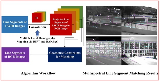
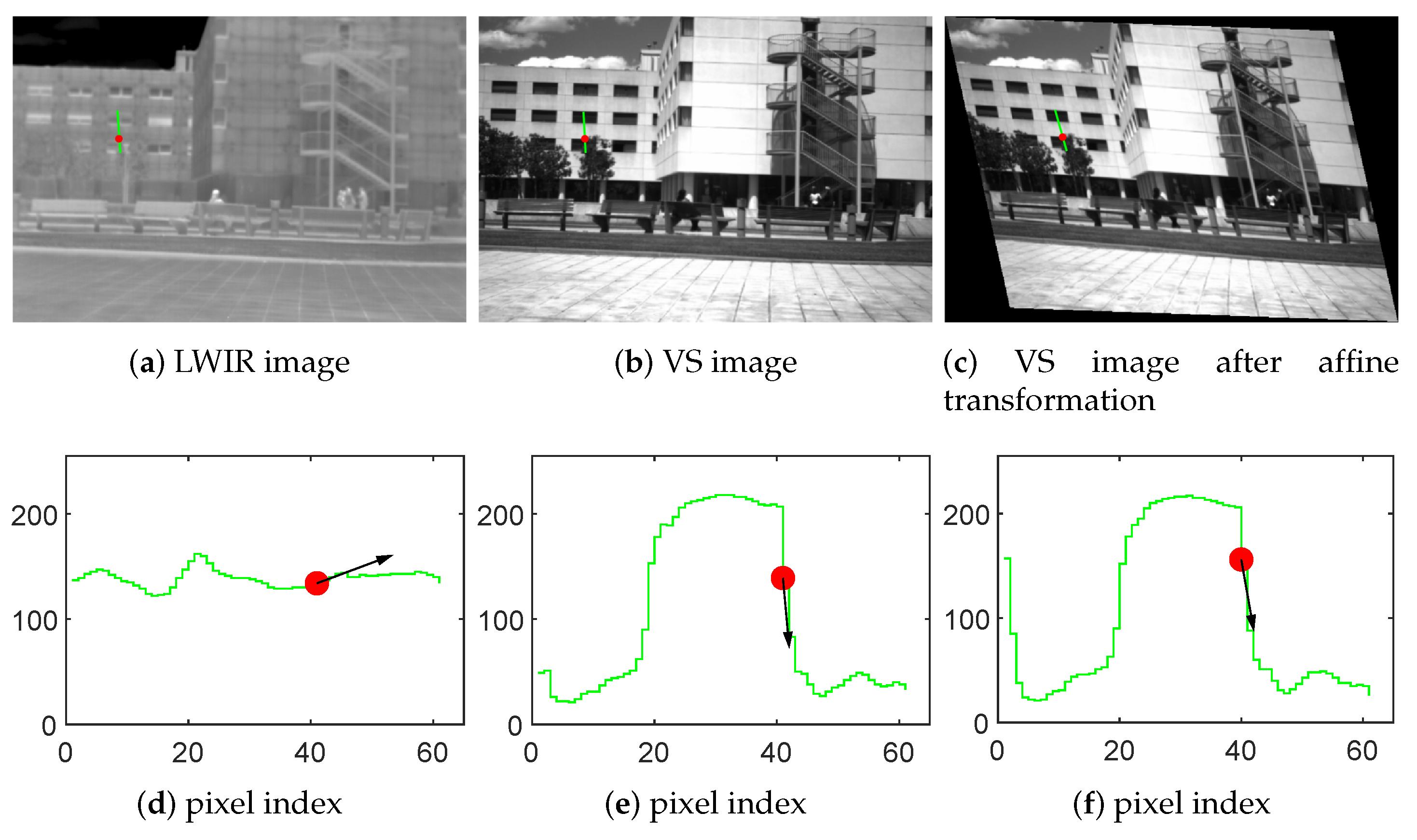
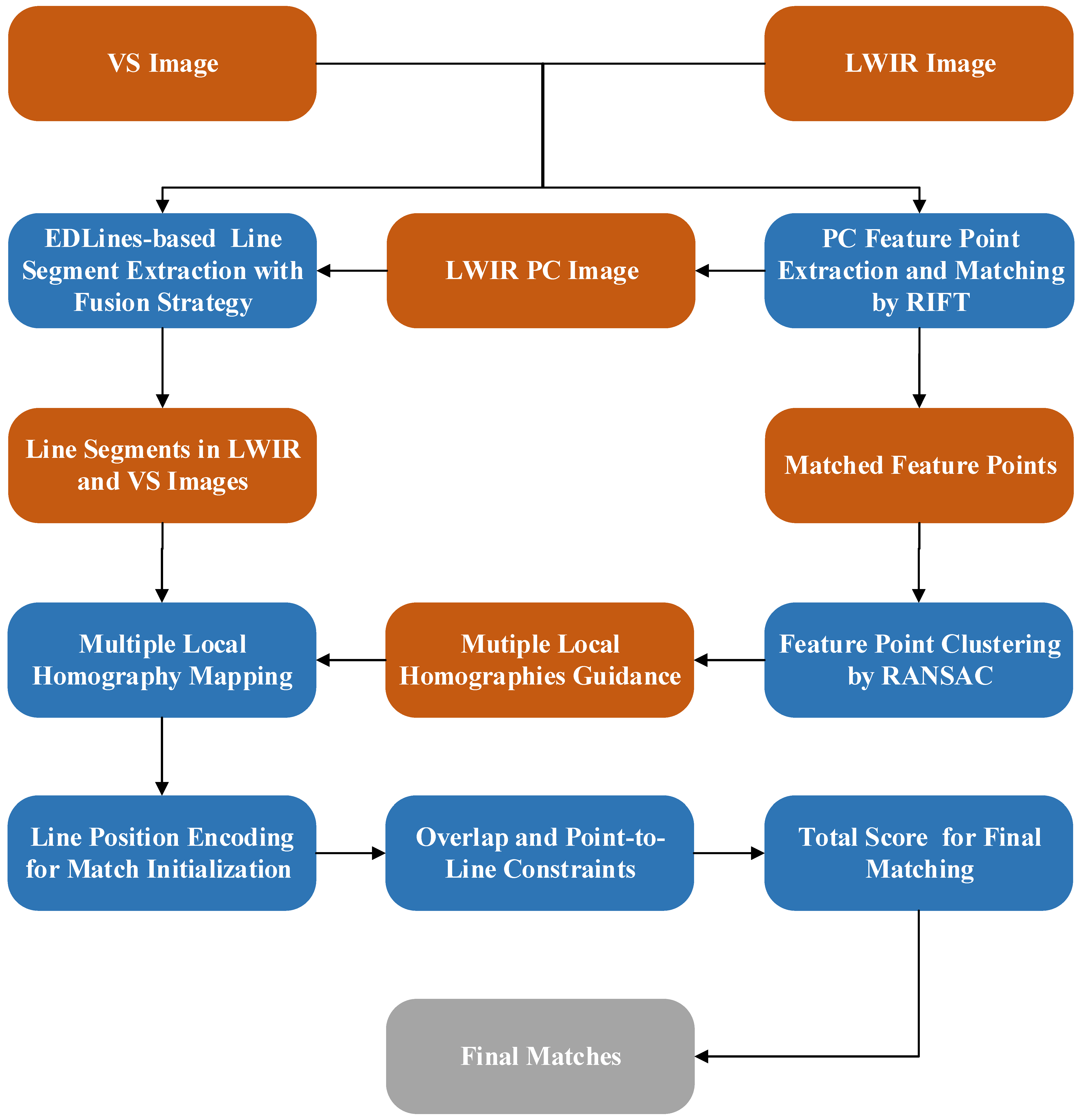
Multispectral feature matching has numerous applications, such as image fusion in satellite remote sensing and IR-VS image fusion in industry and robotics. Nonetheless, NRD can render single-spectral intensity-based matching techniques ineffective [14]. Shen et al. [30] proposed a new matching cost to release the gradient and colour variation in VS/NIR matching. Brown and Susstrunk [31] modified the SIFT descriptor to make it applicable to cross-spectrum matching. However, such methods will invariably fail in VS-LWIR cases in which the wavelength difference between two sensors exceeds the feasible region in which intensity-based matching can work; the gradient histograms could be fairly different (the pixel values of a LWIR image are proportional to the temperature, but this is not the case in VS images). Thus, the invariant attributes (i.e., structure and geometry information) insensitive to the NRD should be adopted for feature matching.

For point matching, Aguilera et al. [32] designed the edge-oriented histogram (EOH) descriptor constructed using the neighbouring edges of the interesting points. First, the keypoints and edge image are extracted. Then, the neighbouring area of these keypoints in the edge image is divided into 4 × 4 sub-regions. After that, five Sobel filters for detecting edges in different directions are implemented to be convoluted with these sub-regions. Thus, a histogram with $5\times 4\times 4$ bins can be used as the descriptor of a keypoint for feature matching. This method fully focused on the local geometric structure so that it still worked even with strong NRD. Aguilera et al. [33] and Nunes et al. [13] have further extended this idea, replacing the simple Sobel filters with Log-Gabor (LG) filters in the frequency domain with different scalars (frequency) and orientations and then building the histogram of the filtering results for point matching. Ma et al. [34] also used similar concepts. Zhao et al. [35] applied phase congruency (PC) [36] to extract the corner and edge images. Then, line segments were extracted from the PC edge images. After the PC process, the pixel values of the PC image were normalized to [0,1] so that the PC images were independent of pixel intensity, which can be helpful for multispectral feature matching. In the next step, local scale-orientation-invariant feature keypoint descriptors were constructed from the relative positions between the centre keypoints and the intensity-independent structures (corners, line segments). Inspired by the important attribute that the PC response of a pixel could simultaneously possess phase, orientation, and magnitude, histogram-oriented phase congruency (HOPC) [37] was proposed for constructing an intensity-like descriptor with the magnitude and orientation of the PC image. Liu et al. [38] modified this concept for affine invariant. Chen et al. [39] also built a SIFT-like rotation-invariant descriptor according to this attribute. RIFT [12] improved the matching performance by using the MIM (maximum index map) for feature description instead of the overall summation of PC responses of a pixel at all orientations and scales. Besides, learning-based multispectral feature point matching has been a new trend in recent years [40,41].

Multispectral line segment matching, on the contrary, has not received as much attention as multispectral point matching because of the challenges introduced in Section 1. First, NRD problem causes the poor performance of individual (intensity-based) line matching approaches such as LBD and MSLD. Thus, only geometry-based or structure-based methods are worthy of consideration [18,42,43]. Li et al. [18] utilized the intersections of line segments as anchors and EOH-based point descriptor for the construction of line segment descriptor. Second, the low texture of LWIR images compared with that of VS images reduces the repeatability of local structures. For point matching, the influence may not be so significant. However, when matching lines, intersection-based or group matching-based approaches introduced before will suffer from a lack of repeatable local line structures. Therefore, the number of matching candidates will largely decrease. Third, most of the introduced multispectral line matching techniques assume that the transformation between two images can be described by a single homography [44], which indicates the existence of a global transformation. However, in man-made scenarios, multiple local homographies usually exist (which means the existence of multiple planes).

In summary, the current line segment matching methods encounter the following three problems in multispectral scenarios: NRD, low texture similarity, and the absence of local transformations. To address these three problems, the proposed method based on PC and multiple local homographies (PC-MLH) uses the matched and clustered multispectral feature points as global guidance, and then the searching space is shrunk via several methods, thereby significantly improving matching accuracy.

3. Methodology

3.1. Feature Point Matching and Clustering

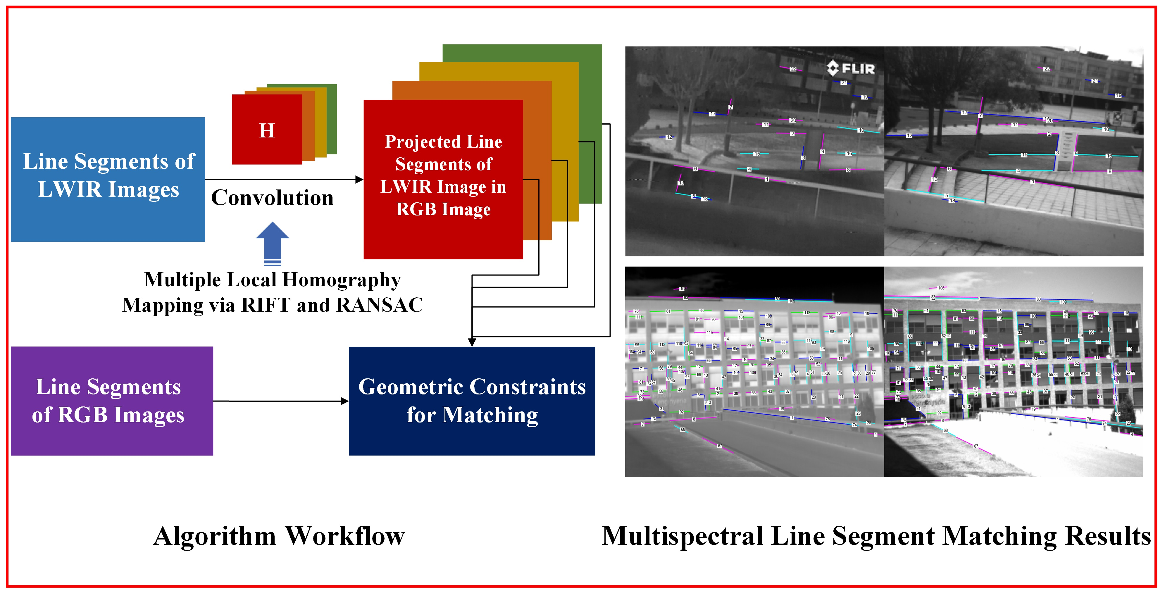
3.1.1. PC and Feature Point Matching

Phase Congruency, first proposed by Kovesi et al. [36], is widely used in multispectral feature extraction and matching. It filters an image in the frequency domain using LG filters with different scales and orientations by

$$L{G}_{m,n}(f,\theta )=exp\left(-\frac{log{(f/f_m)}^2}{2{\left(log({\sigma }_f/f_m)\right)}^2}\right)exp\left(-\frac{{(\theta -{\theta }_n)}^2}{2{\sigma }_{\theta }^2}\right),$$

(1)

where m and n are the local frequency index and the local direction index, respectively. f denotes the frequency and $\theta$ represents the angle. $f_m$ and ${\theta }_n$ are the local centre frequency and local centre direction, respectively. ${\sigma }_f$ and ${\sigma }_{\theta }$ are the width parameters of the frequency and angle, respectively.

In the spatial domain, such LG filters are composed of a real even part $F_{m,n}^e$ and an imaginary odd part $F_{m,n}^o$. The convolution results of the image $I(x,y)$ (where $(x,y)$ is the pixel position) at frequency $f_m$ and direction ${\theta }_n$ can be depicted as two responses $e_{m,n}(x,y)$ and $o_{m,n}(x,y)$ based on $F_{m,n}^e$ and $F_{m,n}^o$:

$$\left[e_{m,n}(x,y),o_{m,n}(x,y)\right]=\left[I(x,y)\ast F_{m,n}^e,I(x,y)\ast F_{m,n}^o\right].$$

(2)

The local amplitude $A_{m,n}(x,y)$ and direction ${\mathsf{\Phi }}_{m,n}(x,y)$ at pixel $(x,y)$ are defined according to the two convolution results above as follows:

$$\begin{array}{cc}\hfill A_{m,n}(x,y)& =\sqrt{e_{m,n}^2(x,y)+o_{m,n}^2(x,y)},\hfill \\ \hfill {\mathsf{\Phi }}_{m,n}(x,y)& =arctan\left(e_{m,n}(x,y),o_{m,n}(x,y)\right).\hfill \end{array}$$

(3)

Then the PC response of a pixel $(x,y)$ is defined as

$$PC(x,y)={\displaystyle \frac{{\sum }_m{\sum }_n{W}_o(x,y)⌊A_{m,n}(x,y)\Delta {\mathsf{\Phi }}_{m,n}(x,y)-T⌋}{{\sum }_m{\sum }_n{A}_{m,n}(x,y)+ϵ}},$$

(4)

where $W_o(x,y)$ represents the weight coefficient, $\Delta {\mathsf{\Phi }}_{m,n}(x,y)$ is the phase deviation, and T is introduced to suppress the influence of noise. $ϵ$ is a parameter to prevent the denominator from being zero. $\lfloor \rfloor$ is set to zero when the value inside is negative. The phase is normalized to $[0,1]$ by the sum of local amplitudes ${\sum }_m{\sum }_n{A}_{m,n}(x,y)$. Therefore, the $PC$ value is insensitive to the intensity change of the images. When a pixel’s PC response is closer to 1, it is more likely to be an edge. The detailed definition and derivation of the above parameters can be found in [36].

Another important property of $PC$ of a pixel is that it also has an orientation [37]. The orientation $O(x,y)$ of the $PC$ of a pixel $(x,y)$ is given as

$$\begin{array}{c}\hfill {sin}_{\mathrm{total}}=\sum _m\sum _n{o}_{m,n}(x,y)sin\left(n\right),\\ \hfill {cos}_{\mathrm{total}}=\sum _m\sum _n{o}_{m,n}(x,y)cos\left(n\right),\\ \hfill O(x,y)=arctan\left({sin}_{\mathrm{total}},{cos}_{\mathrm{total}}\right).\end{array}$$

(5)

Due to the PC response and its orientation of a point in images being stable and unique with different wavelengths, it is better to describe image pixels using PC response instead of intensity and gradient, which are sensitive to NRD, for multispectral feature matching. In the proposed approach, feature points are matched by RIFT [12]. In RIFT, the feature points were detected according to the maximum moment map of the PC map. Then, instead of directly using the PC magnitude and its orientation for matching, the authors built a maximum index map (MIM) that set the pseudo-intensity of every pixel by the index of the orientation with the maximum filtering response. Next, a SIFT-like descriptor was built for every interesting feature point. Such a kind of descriptor is completely constructed by the neighbouring edge structure of a pixel, so that it was very robust to the wavelength change of sensors compared with the descriptor built according to the intensity of neighbouring pixels.

3.1.2. Clustering of the Matched Multispectral Feature Points

The RIFT algorithm is proposed to register the image pairs in the remote-sensing area. In such scenarios, the transformation between two images is always Affinity. Sometimes this Affinity may even degrade to Similarity or Euclidean transformation. Therefore, a single homography is sufficient to describe the global pixel-wise mapping between two images:

$$X_{3\times 1}^{\prime }=H_{3\times 3}{X}_{3\times 1},$$

(6)

where $X_{3\times 1}$ and $X_{3\times 1}^{\prime }$ are the correspondence points in two planes, and $H_{3\times 3}$ is the homography of these two planes. However, when utilizing such a matching approach in man-made structural scenarios, there always exist several dominant planes that have different corresponding homographies for pixel-wise and plane-wise mappings, which means a simple homography does not exist for the global transformation. Thus, the matched feature points should be clustered into different groups according to the reprojection error to obtain different local homographies of different planes. Iterative random sample consensus (RANSAC) [45] is chosen to achieve this goal because of its easy implementation and relatively high clustering accuracy. After obtaining the matched points of a multispectral image pair, RANSAC extracts a set of points that satisfy the homography projection error threshold with the largest number. The points in the set are more likely to belong to the same plane. Then, the selected points are removed from the initial point set, following which the above process is run iteratively for the remaining points. Finally, the matched points are clustered into several groups with their own local homographies.

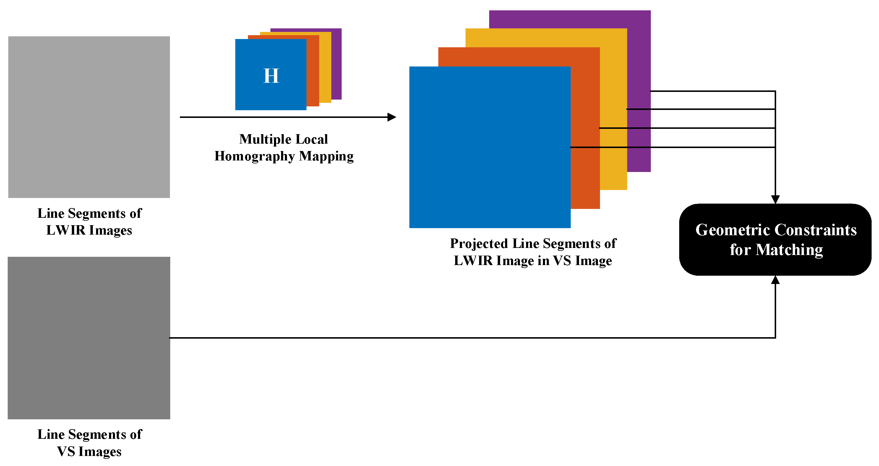
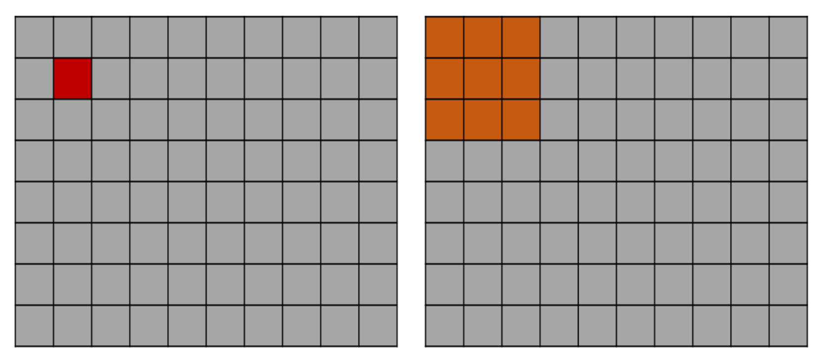
3.2. Line Segment Fusion and Multi-Layer Local Homography Mapping

The line segments in an image are extracted by EDLines [46]. In some cases, the raw IR image demonstrates low texture, and consequently, the line extraction result acquired from the raw IR image (the 2nd image of Figure 3a) is not rich enough compared with the extraction result from its corresponding VS image (the 1st image of Figure 3a). In this case, possible line matching candidates are few, as in Figure 3b. Because PC can emphasize the edge feature, especially in the low-texture area, the line segments extracted from the PC response of the IR image (the 3rd image of Figure 3a) are fused with the line segments extracted from the raw IR image to address this issue. The fused IR line segments are then matched with the line segments in VS images, the 1st image of Figure 3a. The matching result after fusion is shown in Figure 3c, which has more matched pairs compared with Figure 3b.

For a clear description, we define $l_{IR}^i,i=1,2,3,\dots ,p$ as the detected line segments in the IR image and $l_{VS}^j,j=1,2,3,\dots ,q$ as the detected line segments in the VS image. After different local homographies are obtained in the clustering step, the detected line segments $l_{IR}^i$ are mapped into the VS image by different local homographies $H_k^{IR\to VS},k=1,2,3,\dots ,n$ using the formula (6), where n is the number of clustered feature point groups. The mapped line segments are described as $l_{IR,k}^{i,mapped}$. As demonstrated in Figure 4, the line segments in an IR image are mapped into the corresponding VS image according to four local homographies $H_k^{IR\to VS}$, after which each mapped IR line segments by each local homography will be tentatively matched with the neighbouring line segments in the VS image.

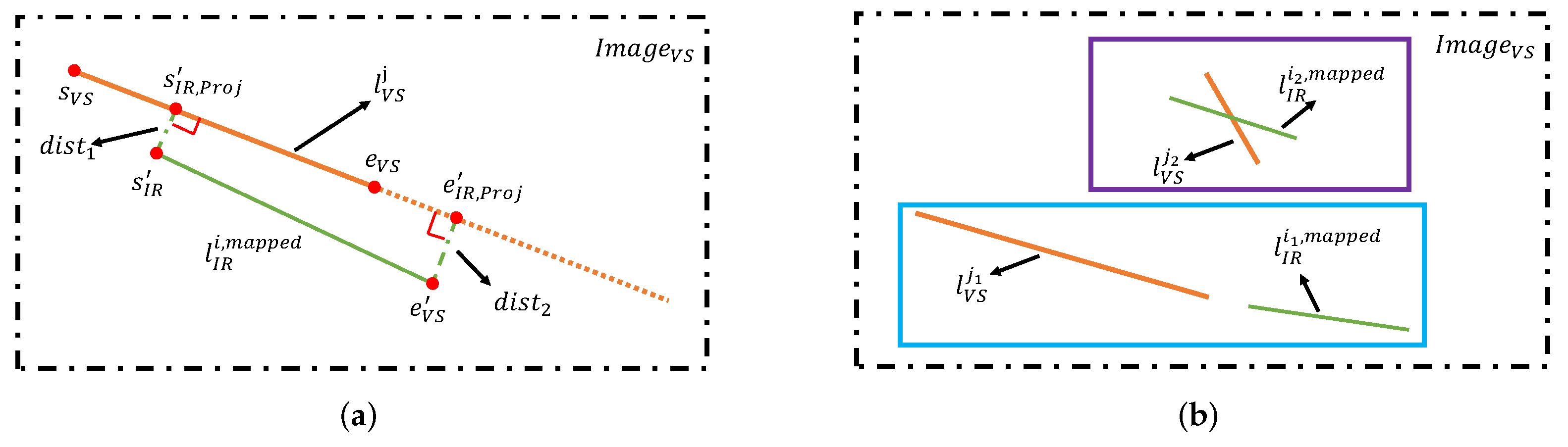
3.3. Geometric Constraints for Matching Candidates Selection

Three geometric constraints (line position constraint, overlap constraint, and point-to-line constraint) and an overall constraint are designed for fast matching with high accuracy. If every line segment in the mapped IR image is to be paired with every line segment in the corresponding VS image, then the total number of constructed line pairs is $p\times q\times n$, where $p,q$ are the number of detected line segments in the IR and VS image, respectively, and n is the number of homography layers. This pairing method is very time-consuming, and many of the line pairs are apparently not matched. However, after mapping the line segments in the IR image into the VS image, the distance between line segment correspondence will not be too far. In this situation, the line segments can be encoded according to their middle point position, as illustrated in Figure 5, and then the mapped line segments $l_{IR,k}^{i,mapped}$ in a bin will only be possible to be paired with the line segments $l_{VS}^j$ scattered in the neighbouring bins. Through this minimal pairing strategy, those line pairs that cannot be matched will not be considered and occupy the computing resource.

Aside from line position encoding, two additional constraints are added for efficient outlier removal: the overlap constraint with the corresponding threshold $T_o$ and the point-to-line distance constraint with the distance threshold $T_d$. First, a matched line pair should have a large proportion of overlapped parts. The startpoint and endpoint of a line segment in the IR image are defined as $s_{IR}$ and $e_{IR}$, respectively ($x_{s_{IR}}<x_{e_{IR}}$). Similarly, $s_{VS}$ and $e_{VS}$ can be defined in the VS image. After local homography transformation, the coordinates of $s_{IR}$ and $e_{IR}$ on the VS image are $s_{IR}^{\prime }$ and $e_{IR}^{\prime }$. For every IR-VS line pair, the two mapped points of the IR line segment are further projected onto the VS line segment: $s_{IR,Proj}^{\prime }$ and $e_{IR,Proj}^{\prime }$. Following this, there are four defined points on the VS line segment of this IR-VS pair $(s_{IR,Proj}^{\prime },e_{IR,Proj}^{\prime },s_{VS},e_{VS})$. The overlapped two line segments in a line pair must satisfy any one of the following two conditions:

$$s_{VS}<e_{IR,Proj}^{\prime }<e_{VS},$$

(7)

or

$$s_{VS}<s_{IR,Proj}^{\prime }<e_{VS}.$$

(8)

Then, the qualified line pairs are used to compute the overlap ratio $R_o$ as follows:

$$R_o={\displaystyle \frac{\parallel \overrightarrow{P_2{P}_3}\parallel }{min(\parallel \overrightarrow{P_1{P}_3}\parallel ,\parallel \overrightarrow{P_2{P}_4}\parallel )}},$$

(9)

where $(P_1,P_2,P_3,P_4)$ are the sorted points of the points set $(s_{VS},s_{IR,Proj}^{\prime },e_{VS},e_{IR,Proj}^{\prime })$ based on their x coordinates: $X_{P_1}<X_{P_2}<X_{P_3}<X_{P_4}$. Only when $R_o>T_o$, is the line pair accepted as a matched candidate, as demonstrated in Figure 6a. If one line segment is fully dropped on another line segment, then $R_{overlap}=1$.

Second, a matched line pair should have a relatively small point-to-line distance, where ‘point’ means the mapped points $s_{IR}^{\prime }$ or $e_{IR}^{\prime }$ and the term ’line’ means the corresponding line segment $l_{VS}^j$ in VS image. The score is calculated as

$$\begin{array}{cc}\hfill D_{p2l}& =\sqrt{dis{t}_1^2+dis{t}_2^2}\hfill \\ \hfill dis{t}_{1,2}& ={\displaystyle \frac{\parallel X^T{l}_{VS}^j\parallel }{\sqrt{a^2+b^2}}},\hfill \end{array}$$

(10)

where $l_{VS}^j={(a,b,1)}^{\prime }$ is the VS line segment of the matching candidate, X is $s_{IR}^{\prime }$ or $e_{IR}^{\prime }$ with the homogeneous coordinate form $X={(x,y,1)}^{\prime }$.

These two constraints are used for separately evaluating the matching candidate from different perspectives and both of them are of importance. If a matching candidate satisfies only one of them, it is very likely to be a false match, as depicted in Figure 6b. However, a correct match does not mean it has an overlap ratio close to 1 and a point-to-line distance close to 0 because of the fragmented line segment extraction and the projection error. Thus, relatively small $T_o$ and large $T_d$ are chosen for initial outlier removal. Then, an extra total evaluation threshold $T_t$ is added to combine the overlap and point-to-line constraints to obtain the final score S of a matching candidate:

$$S=\left\{\begin{array}{cc}{e}^{D_{p2l}}{e}^{\lambda (1-R_o)}& (D_{p2l}<T_d)\wedge (R_o>T_o)\\ \infty & else\end{array}\right.,$$

(11)

where $\lambda$ is a hyper-parameter for adjusting the weight of the two constraints. A matching candidate has n total scores computed from different homography layers. If at least one of them is smaller than the total threshold $T_t$, the candidate $(l_{IR}^i,l_{VS}^j)$ is considered a true matching result.

To further reduce computational complexity, these constraints are set up in cascade. That is, after line position encoding, the overlap ratio is calculated only when two line segments overlap; the point-to-line distance is calculated only when the overlap ratio is greater than the threshold $T_o$; and the total score of this matching candidate is computed only when $D_{p2l}$ is less than the threshold $T_d$. A matching candidate will no longer be considered as long as it does not meet with the associated constraint in any above step. The overall process is shown in Algorithm 1.

Algorithm 1 PC-MLH for Multispectral Line Segment Matching

Input:  Mapped IR line segments in the VS image and VS line segments. Multiple local homographies $H_k,K=1,2,...,n$. Output:  Set of matched pairs 1: Line position encoding strategy based on their middle point positions 2: for Every line segment $l_{IR}^{i,mapped}$ in a bin and the VS line segments $l_{VS}^j$ in the neighbouring bins do 3:     if Two line segments have overlapping parts then 4:         Compute the overlap ratio $R_{overlap}$ 5:         if $R_{overlap}>T_o$ then 6:            Compute the point-to-line distance $D_{p2l}$ 7:            if $D_{p2l}<T_d$ then 8:                Compute the total score S 9:                if $S<T_t$ then 10:                    Save $(l_{IR}^i,l_{VS}^j)$ as a matched pair 11:                end if 12:            end if 13:         end if 14:     end if 15: end for

4. Experiment Results

4.1. Datasets and Evaluation Criterion

The outdoor datasets CVC-Multimodal [47] and VIS-IR [33] (hereafter represented by CVC and VIS for convenience) are used for both qualitative and quantitative evaluation. Because most of the images in the VIS dataset have an apparent dominant plane, while the CVC dataset is a more general scenario with multiple planes existing in an image, the experimental results of these two datasets are separately analysed. To the best of our knowledge, there is seldom open-source codes of the multispectral line segment matching approach in recent years. Therefore, we directly use the statistics in LSM-IM [18] for comparison because it was validated on the same dataset (CVC) used in our experiments. Besides, we also compare the current PC-MLH with some classical matching approaches designed for single-spectrum scenarios (VS-VS). LBD, LJL, and LS are selected as references; these approaches are based on intensity, local structure matching, and group matching, respectively. All of these algorithms use VS-LWIR image pairs in these two datasets as input. A learning-based line matching algorithm is not chosen for comparison because such algorithms are trained by single-spectrum datasets based on the local intensity and therefore do not differ from the traditional intensity-based approaches from the perspective of multispectral line segment matching.

Similar to the previous line segment matching algorithms [1,2,3,18,19,27], the performance indices include the number of detected matches (NDM), the number of correct matches (NCM), and the percentage of correct matches (PCM) that are calculated by NCM/NDM. All of the experiments in this section are carried out on a desktop computer equipped with Intel(R) Core(TM) i7-8700 @ 3.20 GHZ, RAM 32 GB, NVIDIA GEFORCE GTX 1080. The PC-MLH is designed and verified on MATLAB R2021b, while the other three traditional algorithms are tested using open-source codes. Thus, we do not compare the time consumption among them. However, the line segment extraction parts of these four algorithms are all modified to EDLines [46] with the same parameters for performance comparison on the three indices defined above.

4.2. Parameters Analysis

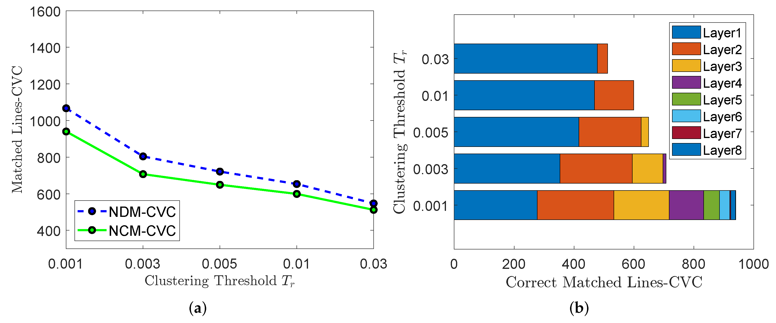
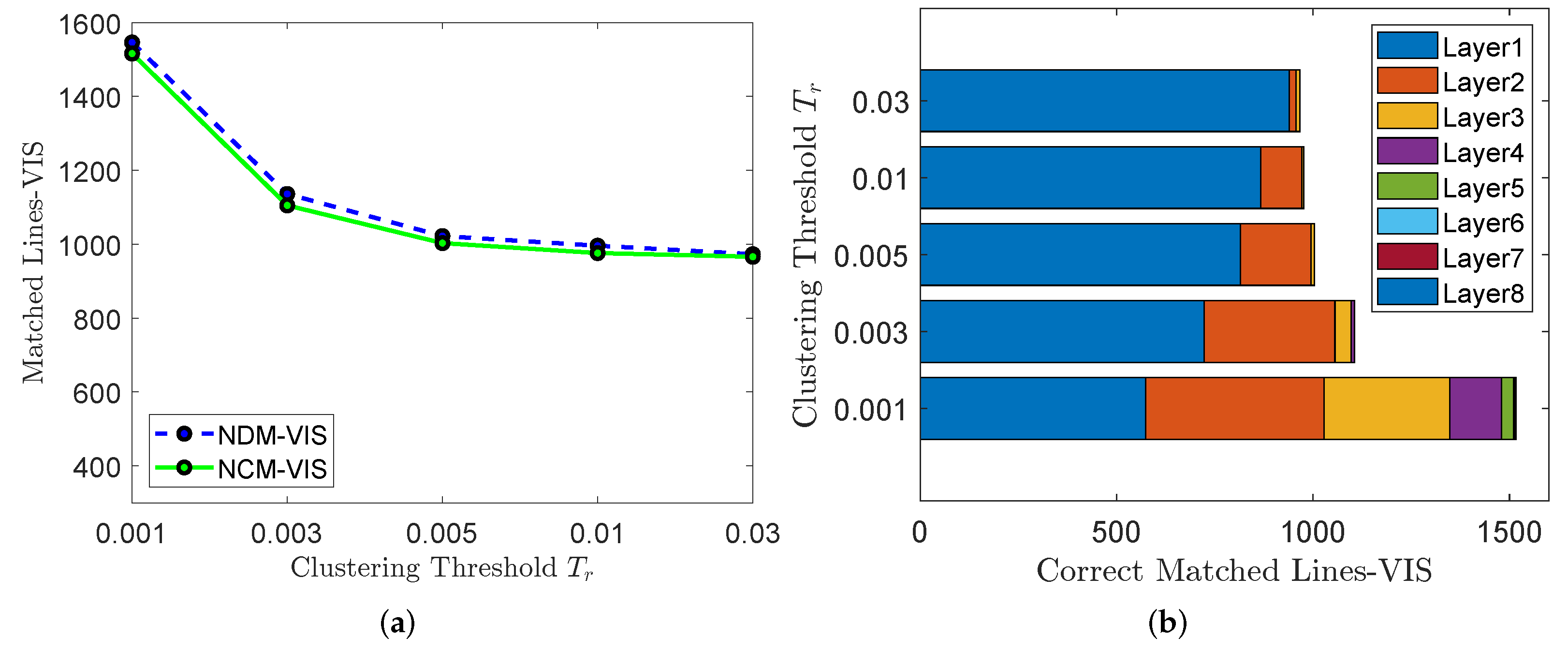
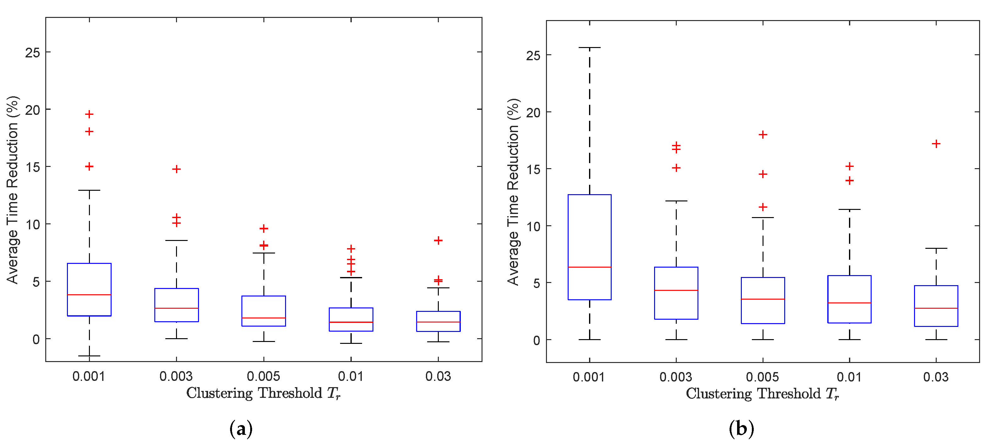
4.2.1. Clustering Threshold $T_r$

In the PC-MLH process of feature point clustering by RANSAC, the clustering threshold $T_r$ should be defined properly for selecting the inlier points that satisfy the current homography model at every iteration step. The point coordinates are normalized with respect to the relative position to the centroid of points used for constructing the local homography, aiming to obtain a more stable clustering result. In the experiments, $T_r$ is set as 0.001–0.03 for comparison. Suppose that the detected feature points set in IR and VS images are $\left\{X_u\right|u=1,2,3,\dots ,o\}$ and $\left\{Y_u\right|u=1,2,3,\dots ,o\}$, respectively, where o is the total number of matched points and $X_u$ and $Y_u$ are the correspondences, the inlier set can now be expressed as

$$Inliers=\left\{(X_u,Y_u)\right|\parallel Y_u-H{X}_u\parallel <T_r,u=1,2,\dots ,o\}.$$

(12)

Table 1. Average number of homography layers (ANHL) with different $T_r$.

	${\mathit{T}}_{\mathit{r}}=0.001$	${\mathit{T}}_{\mathit{r}}=0.003$	${\mathit{T}}_{\mathit{r}}=0.005$	${\mathit{T}}_{\mathit{r}}=0.01$	${\mathit{T}}_{\mathit{r}}=0.03$
ANHL-CVC	3.59	2.15	1.68	1.42	1.06
ANHL-VIS	3.25	1.84	1.40	1.25	1.09
ANHL-ALL	3.49	2.06	1.60	1.37	1.07

shows the average number of homography layers per image in CVC, VIS, and All (combing CVC and VIS) datasets defined by

$$\sum _{i=1}^n{L}_i/n,$$

(13)

where $L_i$ is the number of local homography layers of image i, and n is the total number of images. A relatively large $T_r$ means a high tolerance for the projection error; thus, points are grouped as much as possible in a single iteration step. Consequently, the number of total layers is reciprocally related to $T_r$.

After implementing the proposed PC-MLH on the CVC dataset, the NDM, NCM with different $T_r$ are depicted in Figure 7a. A clear trend can be seen in the figure: a smaller clustering threshold yields more correct line matches while maintaining a high PCM at the same time. From $T_r=0.03$ to $T_r=0.001$, the NCM increases significantly from 512 to 940, while the PCM fluctuates in a narrow range of 87.93–93.6% with an average high value. The distribution of line matches in different local homography layers is demonstrated in Figure 7b. The results prove that such a local homography matching scheme is effective because (1) the average number of homography layers and the NCM are strongly positively correlated, and (2) more matches are detected in the deeper layers when $T_r$ is smaller. At $T_r=0.03$, the average number of homography layers is 1.06 (Table 1), with almost all of the matches in the first layer (blue part in Figure 7b). In this case, the NCM is 512 (Figure 7a), with 92.86% of them in the first layer. The algorithm treats the image transformation as a single homography with one plane. When the threshold gets lower ($T_r=0.005$), the percentage of correct matches in the first layer decreases to approximately 64.2% (Figure 7b), with an NCM of 721 (Figure 7a) and an average number of homography layers of 1.68 (Table 1). At a lower $T_r$ of 0.001, the percentage in the first layer dramatically drops to $29.5\%$, with 27.2% in the second layer, and 19.6% and 12.23% in the third and fourth layer, respectively (Figure 7b). The average number of homography layers rises to 3.59 (Table 1).

Theoretically, if the image pairs are captured indoors with a small depth of field (DOF), the difference in homography between any two planes could be so big that feature points that are spread out on different planes rarely cluster together into the same group. However, when the LWIR-VS image pairs are captured in an outdoor scenario with a very large DOF and the baseline between two cameras is small (which is true for these two datasets), the general projective geometry is degraded to a weak perspective geometry; that is, the homography difference between two planes is relatively small. In this case, feature points belonging to different planes may be grouped into a set as long as the reprojection error according to this homography is less than the clustering threshold. This explains why in these two datasets, different groups of clustered feature points always have an apparent overlapped area. Nevertheless, the local homography scheme still performs well because, for any local area, there exists a local homography with a smaller reprojection error than other homographies. Then, the line matching in this area can be guided by such homography, which is the same process in an indoor scenario.

The effect of $T_r$ on the matching performance of the PC-MLH tested by VIS shows a slightly different result. The NDM and NCM are shown in Figure 8a. As previously mentioned, in many of the images, a dominant plane occupies a large proportion of the image; thus, the homography difference between different layers is tiny, and all of these homographies are close to the real homography transformation. Consequently, the region the PCM located in shifts from $[87.93\%,93.6\%]$ on CVC to $[97.27\%,99.28\%]$ on VIS. Moreover, because the dominant planes of the VIS dataset always have a strong structural texture, the corresponding NDM and NCM are greater than those of CVC for every $T_r$, even though the total number of images is 44, compared with 100 images of CVC. The average number of homography layers and match distribution are given in the second row of Table 1 and Figure 8b, respectively, demonstrating a similar pattern to those of CVC. The percentage of matches in the first layer (blue part in Figure 8b) falls from 94.52% ($T_r=0.3$) to 37.8% ($T_r=0.001$).

4.2.2. Line Detection Threshold and Parameters of Line Position Encoding

To guarantee the credibility of the experiments, during line segment detection using EDLines, the minimum length of detectable line segments $l_{min}$ is set to the same value for different approaches. Too small and too large values of $l_{min}$ are not appropriate because the detected line segments will be fragmented and rare, respectively, which is not only inconsistent with the actual scenario but also has a negative impact on matching performance. After testing under different $l_{min}$, $l_{min}=30$ can get a relatively good result. During line position encoding according to the middle point positions, we set one bin with the size of $20\times 16$. Thus, $l_{IR}^i$ will search the possible matched line $l_{VS}^j$ in the neighbouring $3\times 3$ bins as mentioned in Figure 5 with the size of $(3\times 20)\times (3\times 16)=60\times 48$.

4.2.3. Matching Thresholds $T_o$, $T_d$, $T_t$, $\lambda$

The thresholds of designed three geometric constraints and the hyper-parameter $\lambda$ are strongly related to the final matching quality. Since the case where two line segments do not overlap but still belong to the same line segments is not considered, we assume that matched line segments must have an overlapping proportion greater than $T_o=0.8$. This simple assumption accounts for almost all of the matched line pairs under the previously defined parameter settings. In addition, $T_d$ and $T_t$ are empirically set as 10 and 5, respectively. The weight parameter $\lambda$ is simply set to 1 in the experiments.

4.3. Matching Performance Comparison

Figure 9 presents the matching results of the proposed PC-MLH on the datasets CVC and VIS. Figure 10 compares the performances of various algorithms. They are all fed with VS-LWIR image pairs of these two datasets as input. The NDM, NCM, and PCM of these four approaches (PC-MLH, LS, LBD, LSM-IM) are shown in

Table 2. Performance comparison among different algorithms.

	NDM	NCM	PCM-CVC (%)	PCM-ALL (%)
LBD	838	116	13.55	13.84
LS	2004	727	33.48	36.28
LSM-IM	-	-	67.69	-
PC-MLH	2613	2456	88.10	93.99

. Because LSM-IM only used the CVC dataset, “PCM-CVC (%)” in Table 2 denotes the performance comparison among all of the four algorithms on the CVC dataset, while the last column, “PCM-ALL (%)”, represents the average performance of algorithms except LSM-IM on both the CVC and VIS datasets. A huge performance improvement can be seen by using PC-MLH compared with multispectral matching techniques and traditional matching techniques designed for single-spectrum scenarios.

Among these three approaches, LS shows a relatively reasonable result; it matches the local line group mostly based on the mutual structure information. In some image pairs sharing many similar local line structures in VS and IR images, LS achieves a competitive index: an NDM of 2004 and a PCM of 36.28% (Table 2). However, in most cases, there are few similar local structures between two images, and therefore, their NDM, NCM, and PCM decrease sharply. Another problem existing in LS results because of its group matching scheme is that the wrong matches also occur in the form of groups, as illustrated in Figure 10d marked by blue rectangles. These problems impair the robustness of LS for multispectral line segment matching. In contrast, the LBD is almost fully based on the local intensity of a line segment for matching, and thus underperforms LS. The NDM and PCM are only 838 and 13.84% (Table 2), respectively. This demonstrates that the NRD phenomenon makes it very hard to resort to intensity for multispectral line segment matching.

For the multispectral matching method LSM-IM, different error thresholds (line segment distance) are selected for cumulative comparison. Therefore, we chose the threshold section [0, 5] which is very close to the Point-to-Line distance threshold defined in this proposal, and then the PCM of LSM-IM and PC-MLH on the dataset CVC are comparable within the same error section. The data shows that the PCM of LSM-IM reaches 67.69% (the third row of the Table 2), which is a significant improvement on the accuracy metric compared with single-spectral approaches, but still less than the PCM of PC-MLH, which achieved 88.10% on the CVC dataset. Note that the NDM and NCM are not introduced in LSM-IM, and therefore, only PCM is available.

In the experiments, LJL fails for all the image pairs in both the CVC and VIS datasets. It uses the local structure for junction construction and then uses local intensity for putative junction matching. Thus, it suffers from both the disadvantages of structure-based methods and intensity-based methods. The average number of constructed line junctions and putative matched junctions are 500 and 2, respectively, which is not enough for the following matching process. However, the proposed PC-MLH utilizes the PC for point matching and does not generate the matching result according to the local line structure or intersections, avoiding the NRD problem and the insufficiency of the local structure.

The distributions of computation consumption (the average time, the percentage of time consumed by the RIFT process, the maximum time, the lower quarter time, and the upper quarter time) are given in

Table 3. Time consumption analysis of PC-MLH with different clustering thresholds $T_r$.

Clustering Threshold ${\mathit{T}}_{\mathit{r}}$	Avg. Total (s)	Avg RIFT Consuming (%)	Max. (s)	Lower Quarter (s)	Upper Quarter (s)
CVC-0.001	10.30	91.81	17.59	6.88	12.66
VIS-0.001	13.03	85.61	19.55	10.05	15.09
CVC-0.003	9.54	96.73	14.39	6.72	11.74
VIS-0.003	12.97	97.21	19.20	10.15	15.16
CVC-0.005	9.54	97.13	13.63	6.80	11.89
VIS-0.005	12.80	97.15	19.91	9.96	14.66
CVC-0.01	9.51	97.31	14.09	6.67	11.88
VIS-0.01	12.85	97.36	19.69	10.16	14.83
CVC-0.03	9.45	97.33	13.97	6.70	11.70
VIS-0.03	12.81	97.38	19.97	9.92	14.77

. The data shows that the RIFT feature matching process takes most of the time consumed by this algorithm. Regardless of the clustering threshold $T_r$, the average RIFT time consumption ranges between 85% and 97%, approximately. A large $T_r$ value, which means a small average number of local homography layers, reduces the time need for clustering. Thus, as $T_r$ changes from 0.001 to 0.03, the percentage of the RIFT’s time consumption slightly increases because the time spent on feature point clustering dominates the remain processes, except RIFT feature point matching.

In Section 3.3, line position encoding and another two geometric constraints processed in cascade are implemented for the reduction of computational complexity. Compared with calculating both overlap and point-to-line constraints of every line pair in the IR and VS images, the degree of time reduction because of the above strategy is illustrated in Figure 11. In cases in which the number of detected line segments in image pairs is large, the effect of the cascade strategy will be more significant. In CVC (Figure 11a), the total time decreases slightly. However, in VIS (Figure 11b), with an average large number of detected line segments, such a method shows superiority in time reduction.

4.4. Limitation Analysis

Although much progress has been made by the method proposed in this paper, it also has two main limitations. First, the RIFT [12] is only weak projective-invariant. Consequently, when the mapping between two imagery planes of VS and IR cameras is a heavy projective transformation, the feature matching step may suffer from performance degradation, resulting in possible decrease of the PC-MLH’s performance. Nevertheless, in most cases, weak projective transformation is sufficient to approximately describe the mapping between two imagery planes. Second, as shown in Figure 11 and the second column of Table 3, although the time consumption is reduced by up to 25% via the designed fast matching strategy, the average time consumption per image is still about 10 s. If this algorithm is deployed for real-time applications like SLAM in which the overall time spent on feature extraction, description and matching is around 30~100 ms per frame, further optimization about time complexity needs to be carefully considered.

5. Conclusions

In this paper, a multispectral line segment matching algorithm called PC-MLH (based on PC and multiple local homographies) was proposed for matching line features in image pairs acquired from cameras with different spectral resolutions. We first elaborated on the limitations associated with conventional feature matching methods and the main challenges associated with multispectral line segment matching, and then provided the details of PC-MLH. Multiple local homographies were generated for image transformation based on multispectral feature point matching and clustering. According to the generated local homographies, the line segments in the IR image were mapped into the VS image. Finally, three geometric constraints were implemented in cascade for fast matching. The experiments demonstrated that PC-MLH qualitatively and quantitatively outperformed other single-spectral and multispectral line segment matching methods in terms of the NDM, NCM, and PCM. The time reduction achieved by the fast matching method was also analysed. The future study will investigate how to reduce the overall time consumption of the algorithm for real-time matching applications, match the line segments in the image pairs with a heavy projective transformation, and design an end-to-end learning-based pipeline for multispectral line segment matching.

References

1. Wang, L.; Neumann, U.; You, S. Wide-baseline image matching using line signatures. In Proceedings of the IEEE 12th International Conference on Computer Vision, Kyoto, Japan, 27 September–4 October 2009; pp. 1311–1318. [Google Scholar]
2. Li, K.; Yao, J.; Lu, X.; Li, L.; Zhang, Z. Hierarchical line matching based on line–junction–line structure descriptor and local homography estimation. Neurocomputing 2016, 184, 207–220. [Google Scholar] [CrossRef]
3. Zhang, L.; Koch, R. An efficient and robust line segment matching approach based on LBD descriptor and pairwise geometric consistency. J. Vis. Commun. Image Represent. 2013, 24, 794–805. [Google Scholar] [CrossRef]
4. Zhang, G.; Lee, J.H.; Lim, J.; Suh, I.H. Building a 3-D line-based map using stereo SLAM. IEEE Trans. Robot. 2015, 31, 1364–1377. [Google Scholar] [CrossRef]
5. Gomez-Ojeda, R.; Moreno, F.A.; Zuniga-Noël, D.; Scaramuzza, D.; Gonzalez-Jimenez, J. PL-SLAM: A stereo SLAM system through the combination of points and line segments. IEEE Trans. Robot. 2019, 35, 734–746. [Google Scholar] [CrossRef] [Green Version]
6. Chan, S.H.; Wu, P.T.; Fu, L.C. Robust 2D indoor localization through laser SLAM and visual SLAM fusion. In Proceedings of the 2018 IEEE International Conference on Systems, Man, and Cybernetics (SMC), Miyazaki, Japan, 7–10 October 2018; pp. 1263–1268. [Google Scholar]
7. Chang, L.; Niu, X.; Liu, T.; Tang, J.; Qian, C. GNSS/INS/LiDAR-SLAM integrated navigation system based on graph optimization. Remote Sens. 2019, 11, 1009. [Google Scholar] [CrossRef] [Green Version]
8. Wu, F.; Duan, J.; Ai, P.; Chen, Z.; Yang, Z.; Zou, X. Rachis detection and three-dimensional localization of cut off point for vision-based banana robot. Comput. Electron. Agric. 2022, 198, 107079. [Google Scholar] [CrossRef]
9. Wang, H.; Lin, Y.; Xu, X.; Chen, Z.; Wu, Z.; Tang, Y. A Study on Long-Close Distance Coordination Control Strategy for Litchi Picking. Agronomy 2022, 12, 1520. [Google Scholar] [CrossRef]
10. Khattak, S.; Papachristos, C.; Alexis, K. Visual-thermal landmarks and inertial fusion for navigation in degraded visual environments. In Proceedings of the IEEE Aerospace Conference, Big Sky, MT, USA, 2–9 March 2019; pp. 1–9. [Google Scholar]
11. Chen, L.; Sun, L.; Yang, T.; Fan, L.; Huang, K.; Xuanyuan, Z. Rgb-t slam: A flexible slam framework by combining appearance and thermal information. In Proceedings of the IEEE International Conference on Robotics and Automation (ICRA), Singapore, 29 May–3 June 2017; pp. 5682–5687. [Google Scholar]
12. Li, J.; Hu, Q.; Ai, M. RIFT: Multi-modal image matching based on radiation-variation insensitive feature transform. IEEE Trans. Image Process. 2019, 29, 3296–3310. [Google Scholar] [CrossRef]
13. Nunes, C.F.; Pádua, F.L. A local feature descriptor based on log-Gabor filters for keypoint matching in multispectral images. IEEE Geosci. Remote Sens. Lett. 2017, 14, 1850–1854. [Google Scholar] [CrossRef]
14. Li, S.; Lv, X.; Ren, J.; Li, J. A Robust 3D Density Descriptor Based on Histogram of Oriented Primary Edge Structure for SAR and Optical Image Co-Registration. Remote Sens. 2022, 14, 630. [Google Scholar] [CrossRef]
15. Wang, Z.; Wu, F.; Hu, Z. MSLD: A robust descriptor for line matching. Pattern Recognit. 2009, 42, 941–953. [Google Scholar] [CrossRef]
16. Verhagen, B.; Timofte, R.; Van Gool, L. Scale-invariant line descriptors for wide baseline matching. In Proceedings of the IEEE Winter Conference on Applications of Computer Vision, Steamboat Springs, CO, USA, 24–26 March 2014; pp. 493–500. [Google Scholar]
17. Li, K.; Yao, J. Line segment matching and reconstruction via exploiting coplanar cues. ISPRS J. Photogramm. Remote Sens. 2017, 125, 33–49. [Google Scholar] [CrossRef]
18. Li, Y.; Wang, F.; Stevenson, R.; Fan, R.; Tan, H. Reliable line segment matching for multispectral images guided by intersection matches. IEEE Trans. Circuits Syst. Video Technol. 2019, 29, 2899–2912. [Google Scholar] [CrossRef]
19. Chen, M.; Yan, S.; Qin, R.; Zhao, X.; Fang, T.; Zhu, Q.; Ge, X. Hierarchical line segment matching for wide-baseline images via exploiting viewpoint robust local structure and geometric constraints. ISPRS J. Photogramm. Remote Sens. 2021, 181, 48–66. [Google Scholar] [CrossRef]
20. Lowe, D.G. Distinctive image features from scale-invariant keypoints. Int. J. Comput. Vis. 2004, 60, 91–110. [Google Scholar] [CrossRef]
21. Bay, H.; Tuytelaars, T.; Gool, L.V. Surf: Speeded up robust features. In Proceedings of the European Conference on Computer Vision, Graz, Austria, 7–13 May 2006; pp. 404–417. [Google Scholar]
22. Rublee, E.; Rabaud, V.; Konolige, K.; Bradski, G. ORB: An efficient alternative to SIFT or SURF. In Proceedings of the International Conference on Computer Vision, Barcelona, Spain, 6–13 November 2011; pp. 2564–2571. [Google Scholar]
23. DeTone, D.; Malisiewicz, T.; Rabinovich, A. Superpoint: Self-supervised interest point detection and description. In Proceedings of the IEEE Conference on Computer Vision and Pattern Recognition, Salt Lake City, UT, USA, 18–23 June 2018; pp. 224–236. [Google Scholar]
24. Fan, B.; Wu, F.; Hu, Z. Robust line matching through line–point invariants. Pattern Recognit. 2012, 45, 794–805. [Google Scholar] [CrossRef]
25. Al-Shahri, M.; Yilmaz, A. Line matching in wide-baseline stereo: A top-down approach. IEEE Trans. Image Process. 2014, 23, 4199–4210. [Google Scholar]
26. Jia, Q.; Gao, X.; Fan, X.; Luo, Z.; Li, H.; Chen, Z. Novel coplanar line-points invariants for robust line matching across views. In Proceedings of the European Conference on Computer Vision, Amsterdam, The Netherlands, 11–14 October 2016; pp. 599–611. [Google Scholar]
27. Wang, J.; Zhu, Q.; Liu, S.; Wang, W. Robust line feature matching based on pair-wise geometric constraints and matching redundancy. ISPRS J. Photogramm. Remote Sens. 2021, 172, 41–58. [Google Scholar] [CrossRef]
28. Lange, M.; Schweinfurth, F.; Schilling, A. Dld: A deep learning based line descriptor for line feature matching. In Proceedings of the 2019 IEEE/RSJ International Conference on Intelligent Robots and Systems (IROS), Macau, China, 3–8 November 2019; pp. 5910–5915. [Google Scholar]
29. Zhang, H.; Luo, Y.; Qin, F.; He, Y.; Liu, X. ELSD: Efficient Line Segment Detector and Descriptor. In Proceedings of the IEEE/CVF International Conference on Computer Vision, Montreal, QC, Canada, 11–17 October 2021; pp. 2969–2978. [Google Scholar]
30. Shen, X.; Xu, L.; Zhang, Q.; Jia, J. Multi-modal and multi-spectral registration for natural images. In Proceedings of the European Conference on Computer Vision, Zurich, Switzerland, 6–12 September 2014; pp. 309–324. [Google Scholar]
31. Brown, M.; Süsstrunk, S. Multi-spectral SIFT for scene category recognition. In Proceedings of the IEEE Computer Vision and Pattern Recognition (CVPR), Colorado Springs, CO, USA, 20–25 June 2011; pp. 177–184. [Google Scholar]
32. Aguilera, C.; Barrera, F.; Lumbreras, F.; Sappa, A.D.; Toledo, R. Multispectral image feature points. Sensors 2012, 12, 12661–12672. [Google Scholar] [CrossRef] [Green Version]
33. Aguilera, C.A.; Sappa, A.D.; Toledo, R. LGHD: A feature descriptor for matching across non-linear intensity variations. In Proceedings of the IEEE International Conference on Image Processing (ICIP), Quebec City, QC, Canada, 27–30 September 2015; pp. 178–181. [Google Scholar]
34. Ma, T.; Ma, J.; Yu, K. A local feature descriptor based on oriented structure maps with guided filtering for multispectral remote sensing image matching. Remote Sens. 2019, 11, 951. [Google Scholar] [CrossRef] [Green Version]
35. Zhao, C.; Zhao, H.; Lv, J.; Sun, S.; Li, B. Multimodal image matching based on multimodality robust line segment descriptor. Neurocomputing 2016, 177, 290–303. [Google Scholar] [CrossRef]
36. Kovesi, P. Image features from phase congruency. Videre J. Comput. Vis. Res. 1999, 1, 1–26. [Google Scholar]
37. Ye, Y.; Shan, J.; Bruzzone, L.; Shen, L. Robust registration of multimodal remote sensing images based on structural similarity. IEEE Trans. Geosci. Remote Sens. 2017, 55, 2941–2958. [Google Scholar] [CrossRef]
38. Liu, X.; Ai, Y.; Zhang, J.; Wang, Z. A novel affine and contrast invariant descriptor for infrared and visible image registration. Remote Sens. 2018, 10, 658. [Google Scholar] [CrossRef] [Green Version]
39. Chen, H.; Xue, N.; Zhang, Y.; Lu, Q.; Xia, G.S. Robust visible-infrared image matching by exploiting dominant edge orientations. Pattern Recognit. Lett. 2019, 127, 3–10. [Google Scholar] [CrossRef]
40. Aguilera, C.A.; Aguilera, F.J.; Sappa, A.D.; Aguilera, C.; Toledo, R. Learning cross-spectral similarity measures with deep convolutional neural networks. In Proceedings of the IEEE Conference on Computer Vision and Pattern Recognition Workshops, Las Vegas, NV, USA, 26 June–1 July 2016; pp. 1–9. [Google Scholar]
41. Aguilera, C.A.; Sappa, A.D.; Aguilera, C.; Toledo, R. Cross-spectral local descriptors via quadruplet network. Sensors 2017, 17, 873. [Google Scholar] [CrossRef] [PubMed] [Green Version]
42. Li, Y.; Stevenson, R.L. Multimodal image registration with line segments by selective search. IEEE Trans. Cybern. 2016, 47, 1285–1298. [Google Scholar] [CrossRef] [PubMed]
43. Fan, C.; Jin, H.; Wang, F.; Zhang, G.; Li, Y. Combining and matching keypoints and lines on multispectral images. Infrared Phys. Technol. 2019, 96, 316–324. [Google Scholar] [CrossRef]
44. Wang, J.; Liu, S.; Zhang, P. A New Line Matching Approach for High-Resolution Line Array Remote Sensing Images. Remote Sens. 2022, 14, 3287. [Google Scholar] [CrossRef]
45. Fischler, M.A.; Bolles, R.C. Random sample consensus: A paradigm for model fitting with applications to image analysis and automated cartography. Commun. ACM 1981, 24, 381–395. [Google Scholar] [CrossRef]
46. Akinlar, C.; Topal, C. EDLines: A real-time line segment detector with a false detection control. Pattern Recognit. Lett. 2011, 32, 1633–1642. [Google Scholar] [CrossRef]
47. Barrera, F.; Lumbreras, F.; Sappa, A.D. Multispectral piecewise planar stereo using Manhattan-world assumption. Pattern Recognit. Lett. 2013, 34, 52–61. [Google Scholar] [CrossRef]
Figure 1. Visualization of nonlinear radiation distortion (NRD) with the red points being the same location in the environment. (df) show the intensity change near the red points in the image (ac) parallel to the gradient direction from top to down.
Remotesensing 14 03857 g001
Figure 2. Workflow of the proposed multispectral line segment matching method (data, algorithms, and results are enclosed in orange, blue, and grey boxes, respectively).
Remotesensing 14 03857 g002
Figure 3. Illustration of line segment fusion results. (a) Line segment detected in VS, IR image, and PC of IR image. (b) Matching result using VS and IR images. (c) Matching result after line segment fusion.
Remotesensing 14 03857 g003
Figure 4. Illustration of multiple local homographies for matching line segments in IR and VS images.
Remotesensing 14 03857 g004
Figure 5. Line position encoding for fast matching. Left: position grid of the mapped lines of the IR image in the VS image; Right: position grid of the lines in the VS image. Mapped line segments with the middle points located in the red bin will only be paired with the VS line segments with the middle points located in the neighbouring nine orange bins for further evaluation.
Remotesensing 14 03857 g005
Figure 6. Geometric constraints illustration (a) and two examples of false match (b) that only satisfy one of the two geometric constraints. (The matching candidate enveloped with a blue rectangle only satisfies the point-to-line constraint. Another candidate in the purple rectangle only agrees with the overlap threshold).
Remotesensing 14 03857 g006
Figure 7. The influence of different T r on algorithm performance on the CVC dataset. (a) NDM, NCM of the CVC dataset, (b) layer distribution of the CVC dataset.
Remotesensing 14 03857 g007
Figure 8. The influence of different T r on algorithm performance on the VIS dataset. (a) NDM and NCM of the VIS dataset, (b) layer distribution of the VIS dataset.
Remotesensing 14 03857 g008
Figure 9. Demonstration of matching results of the PC-MLH (different colours mean that the matched lines are detected from different local homography layers). The images in the 1st and 3rd columns belong to LWIR images, and those in the 2nd and 4th columns are VS ones.
Remotesensing 14 03857 g009
Figure 10. Performance comparison of PC-MLH, LS, and LBD on two LWIR-VS image pairs. In (af), the left and right images are LWIR and VS images, respectively. (a,c,e) are the results of image pair 1; (b,d,f) are the results of image pair 2. Both of the VS and LWIR images were converted to corresponding greyscale images before the process of line segment extraction.
Remotesensing 14 03857 g010
Figure 11. Time reduction via line position encoding and cascade matching strategies. (a) Time reduction for the CVC dataset, (b) Time reduction for the VIS dataset.
Remotesensing 14 03857 g011