1. Introduction
Even though cities cover less than 5% of the US land surface [
1] and 0.5% of global land cover [
2], urban air quality has become a universal concern. As of 2018, the urban population has swelled to 55% of the world’s population and is projected to reach up to 68% by the year 2050 [
3]. This increased rate of urbanization is accompanied by an increased volume of motorized traffic, industrialization, energy use, and consequently an increase in air pollution [
4,
5,
6]. Long-term exposure to air pollution has been shown to be associated with significant adverse health effects [
7,
8,
9,
10], and is ranked as one of the top five risk factors for mortality of the past two decades [
11]. The effects of air quality are not only reflected in human health, but also in plants and vegetation. Plant injury and damage due to air pollution were discovered as early as the 1870s [
12], and have been extensively studied throughout the past century [
13,
14,
15,
16].
Increased atmospheric particulate matter with diameter less than 2.5 μm (PM
2.5) has shown a significant negative correlation with biochemical parameters in plants, a reduction in stomata and chlorophyll content, as well as increased stress-induced enzyme activity [
17,
18,
19]. These effects are reflected in plants’ photosynthetic rates, which have been detected at rates 50% lower in industrial areas high in PM
2.5 relative to those in control areas [
20]. Adverse effects on tree biomass and visible leaf injury have also been shown to be caused by surface ozone (
), which results in decreased chlorophyll content and, therefore, decreased photosynthesis [
21,
22,
23,
24]. These harmful effects have been discovered in agricultural crops [
25,
26] and forests [
27,
28,
29].
However, it is important to note that studies assessing ozone damage to vegetation are traditionally conducted under controlled environmental conditions using plant chambers to expose plants to known
concentrations [
30,
31]. The numerous variables that compose the environment in urban areas have complex correlations, covariances, and dependencies that can significantly change their expected impact on urban vegetation. For example, studies on the impact of ambient
concentrations on urban vegetation suffer from the inability to separate the effects of
from those of other urban pollutants and stressors using direct observations mainly due to the nature of ozone not accumulating in plant tissue or causing any unique signatures [
32,
33], as well as the need for
concentrations to exceed 200–300 ppb for their effects to be measurable in vegetation [
28]. Furthermore, strong correlations between
concentrations and surface temperatures have been uncovered over multiple time-scales [
34,
35,
36]. These correlations are made more complex with the existence of PM
2.5 and humidity levels, as well as the occurrence of the urban heat island effect, urban winds, and numerous other natural and anthropogenic factors [
37,
38].
Moreover, plant phenology, the seasonally recurring patterns of environment-mediated growth and development of plants, is heavily dependent on changes in temperature and moisture. Temperature is often regarded as the primary trigger of the timing of plant phenological events [
39,
40]. Leaf spring unfolding, blooming and flowering, and coloring and falling in autumn are processes mainly controlled by changes in temperature. Low temperatures activate plant stress response and induce endodormancy, and a certain accumulated amount of chilling breaks endodormancy and leads to ecodormancy, while the accumulation of warm temperatures accelerates plant cell growth [
41]. Due to climate change and rising global temperatures, studies have reported significant advances in spring unfolding [
42], a shift to earlier blooming [
43], and a delay in autumn leaf coloring [
44]. These effects are further exacerbated in cities due to the urban heat island effect [
45]. Furthermore, studies have shown that moisture and humidity act as potential secondary triggers to various phenological events, including the timing of spring and autumn phenology [
46,
47], and flowering cycles [
48]. Although detailed investigations are lacking, urbanization has a measurable impact on air humidity, precipitation, runoff, and groundwater retention, which has been found to influence plant phenology [
49,
50].
The traditional practice for obtaining data on vegetation health, phenological changes, and vegetation diversity is through physical sample collection and ground-based in situ observations [
50,
51]. These methods remain highly valuable as they provide first-hand direct evidence of vegetation health, and record accurate species and site information. However, in situ observations tend to be uneven in distribution as they often require different observers and can vary in methodology and rigor. In the past two decades, Hyperspectral Imaging (HSI) has emerged as a non-invasive, near real-time tool for evaluating and monitoring the condition of vegetation [
52,
53,
54]. Modern hyperspectral imaging acquires images in several hundred to thousands of spectral bands, thus allowing for a detailed spectral curve to be obtained for each spatial pixel in the image [
55]. This increase in spectral resolution has been used in the studies of vegetation for the detection of disease symptoms and pests [
56,
57,
58], as well as monitoring plant health, stress conditions, and nutrient deficiency [
59,
60,
61]. Since air quality has a measurable effect on the morphological, physiological, and phenological properties of vegetation, these effects are reflected in the spectra of the vegetation, and therefore detectable using vegetation indices such as the Normalized Difference Vegetation Index (NDVI) [
62] or the Photochemical Reflectance Index (PRI) [
63] extracted from hyperspectral imaging. For example, in a 2019 study, [
64] used aerial hyperspectral data (HyMap—126 spectral bands spanning 0.45–2.5 μm, and 5 m spatial resolution) to derive forest health status, using the Red Edge Position (REP) index and Structure-Insensitive Pigment Index (SITI), and showed a correlation between plant health and measured atmospheric dust depositions. Their results showed a statistically significant relationship between increased levels of elements associated with coal mining and combustion and decreased forest health.
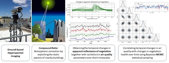
At present, there have been no studies exploring the effects of air quality on urban vegetation via simultaneous measurements at high temporal frequency on the order of minutes for an extended temporal baseline of months. Therefore, in this work, we examine the temporal correlation between changes in air quality measures—namely,
, PM
2.5, temperature, and humidity—and the changes in the spectra of vegetation in ground-based, side-facing HSI images of an urban environment at high spatial, spectral, and temporal resolutions. In
Section 2, we give a brief overview of remote sensing for vegetation health and then present our high-resolution HSI data and the method used for atmospheric correction, the air quality measurements used in this work, and the models used to quantify the correlation between the vegetation spectra and air quality. In
Section 3, we present our results, we provide a discussion of their implications in
Section 4, and summarize our conclusions in
Section 5.
2. Materials and Methods
The literature on remote sensing of vegetation is dominated by the use of satellite, aerial, and, more recently, Unmanned Aerial Vehicle (UAV) imaging platforms. Satellite remote sensing platforms offer the benefits of enhanced spatial coverage and consistent data quality, making them cost-effective, particularly due to open access to a wealth of visible and multispectral data from some satellite platforms (e.g., Landsat 7–8) on which to base analyses [
65]. However, satellite remote sensing also has its limitations, including the lack of high spatial resolution. For example, two of the most commonly used satellite datasets are Landsat and MODIS that have spatial resolutions of 30 m × 30 m and 500 m × 500 m per pixel, respectively. The coarse spatial resolution limits the ability to carry out precision urban agriculture studies, and makes the interpretation of vegetation health challenging when studying mixed canopies with a variety of species co-occurring with different phenological stages and health conditions [
66]. Another limiting factor for satellite-based remote sensing is low temporal resolution, with “revisit time” for a given location typically on the order of days to several weeks (e.g., Landsat has an orbital period of 16 days). This is further exacerbated by potential obscuration by clouds, snow, and ice, that can yield revisits that stretch to months in some cases. The implication is that satellite remote sensing is useful for long-term phenological and land use studies, but lacks the temporal and spatial granularity to study the relationship between urban vegetation and environmental factors that can vary significantly over short spatial and temporal scales, on the order of meters and minutes, respectively, in urban areas. Airborne and UAV platforms have the potential to solve some of these problems, however, due to the requirement of expensive aircraft and trained pilots, airborne platforms can be significantly cost prohibitive and, due to weather dependency, low data transfer speeds (particularly for high-resolution images), and legislative barriers for UAV platforms, neither is capable of collecting persistent data with high temporal granularity.
For the direct measurement of atmospheric and ecological variables at high spatial and temporal resolutions in forests and agriculture, “proximal sensing” by flux towers is normally employed. Flux towers are antenna-mounted arrays of multiple sensors that can observe temperature, humidity, atmospheric gases, atmospheric pollutants, and dust concentrations [
67]. Flux towers have also been installed in urban areas to study issues such as the urban heat island effect, climate forecasting, air quality, and yardscape water demands and consumption [
68]. However, to correlate these measurements with plant and vegetation health, studies either rely on indirect measurements such as evapotranspiration rates, or on using Photosynthetically Active Radiation (PAR) sensors which solely measure photosynthetic processes. To address these shortcomings, ground-based hyperspectral remote sensing has been employed over the past decade [
69,
70,
71]. These near-surface ground-based hyperspectral cameras further add to vegetation health and phenology studies due to their ability to continuously retrieve images and spectra at a high temporal frequency, and on landscape or species spatial levels.
2.1. Hyperspectral Imaging Data
The Hyperspectral Imaging (HSI) data used in this work were obtained by the “Urban Observatory” (UO) facility in New York City (NYC) [
71,
72,
73,
74]. The UO has deployed broadband visible and infrared imaging cameras, as well as Visible and Near-Infrared (VNIR) and Long Wave Infrared (LWIR) HSI cameras that continuously image landscapes in NYC with high persistence and temporal resolution on the order of minutes. For this work, we use the VNIR instrument described in [
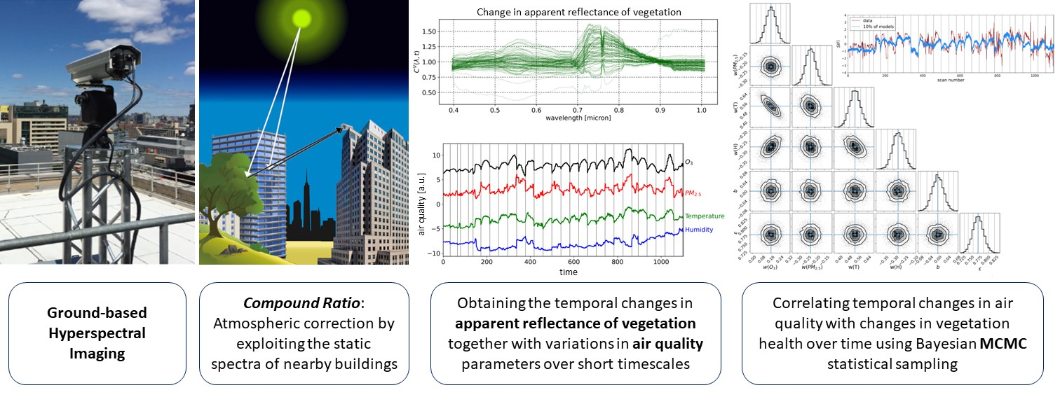
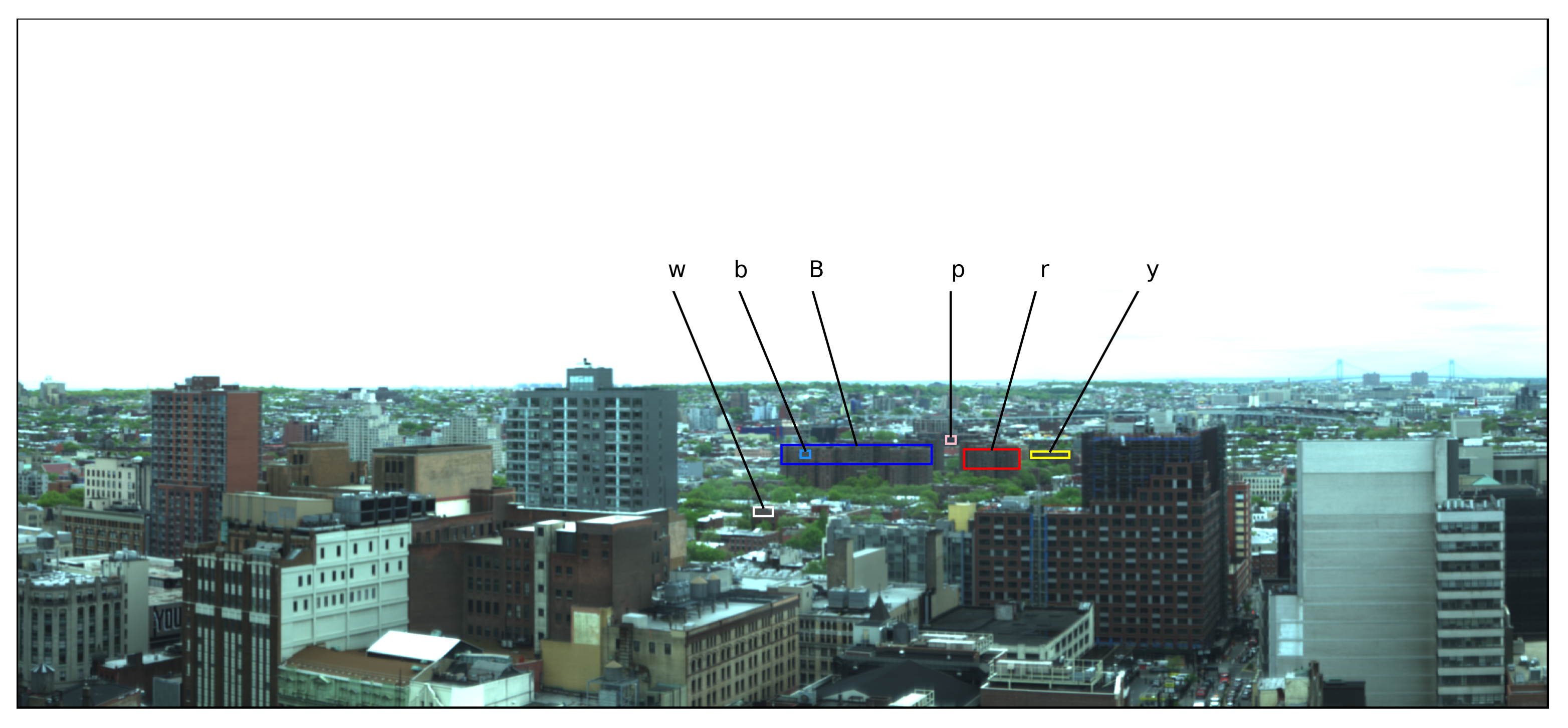
73], a Specim Ltd. ImSpector V10E Visible Near-Infrared (VNIR) hyperspectral imager provided by Middleton Spectral Vision mounted atop a tall ~120 m (~400 ft) building in Brooklyn with a south-facing horizontal alignment. This instrument is a single slit scanning spectrograph with 1600 vertical pixels and is sensitive to 0.4 μm to 1.0 μm in 848 binned wavelength channels with a characteristic spectral resolution (full width half maximum) of 0.72 nm. The observations covered 30 days between 3 May and 6 June 2016. Each day, the instrument scanned the same scene every 15 min from 08h00 to 18h00. Scans with more than 5% of their pixels having more than 5% of their wavelengths saturated were discarded from the sample. A composite RGB image of the scene that maps the 0.61 μm, 0.54 μm, and 0.48 μm channels of one of the scans to the red, green, and blue values, respectively, is shown in
Figure 1.
The scene shown in
Figure 1 contains a variety of materials including sky, clouds, plant material, water, windows, concrete, bricks, metal structures, cars, and roads, and in this work we “segment” our HSI images to isolate those pixels corresponding to vegetation so that we can compare their temporal evolution with time series of air quality measures. Image segmentation of HSI data of dense urban areas is a difficult task given the complexity of the scene, particularly for side-facing images. Advanced deep learning algorithms have been developed and implemented to carry out this segmentation in the literature [
75,
76], however, as shown in [
74], due to the uniqueness of the spectra of vegetation relative to all other urban materials, their identification is particularly robust across a variety of scenes and observational conditions, even with a single training instance when training a One-Dimensional Convolutional Neural Network (1D-CNN).
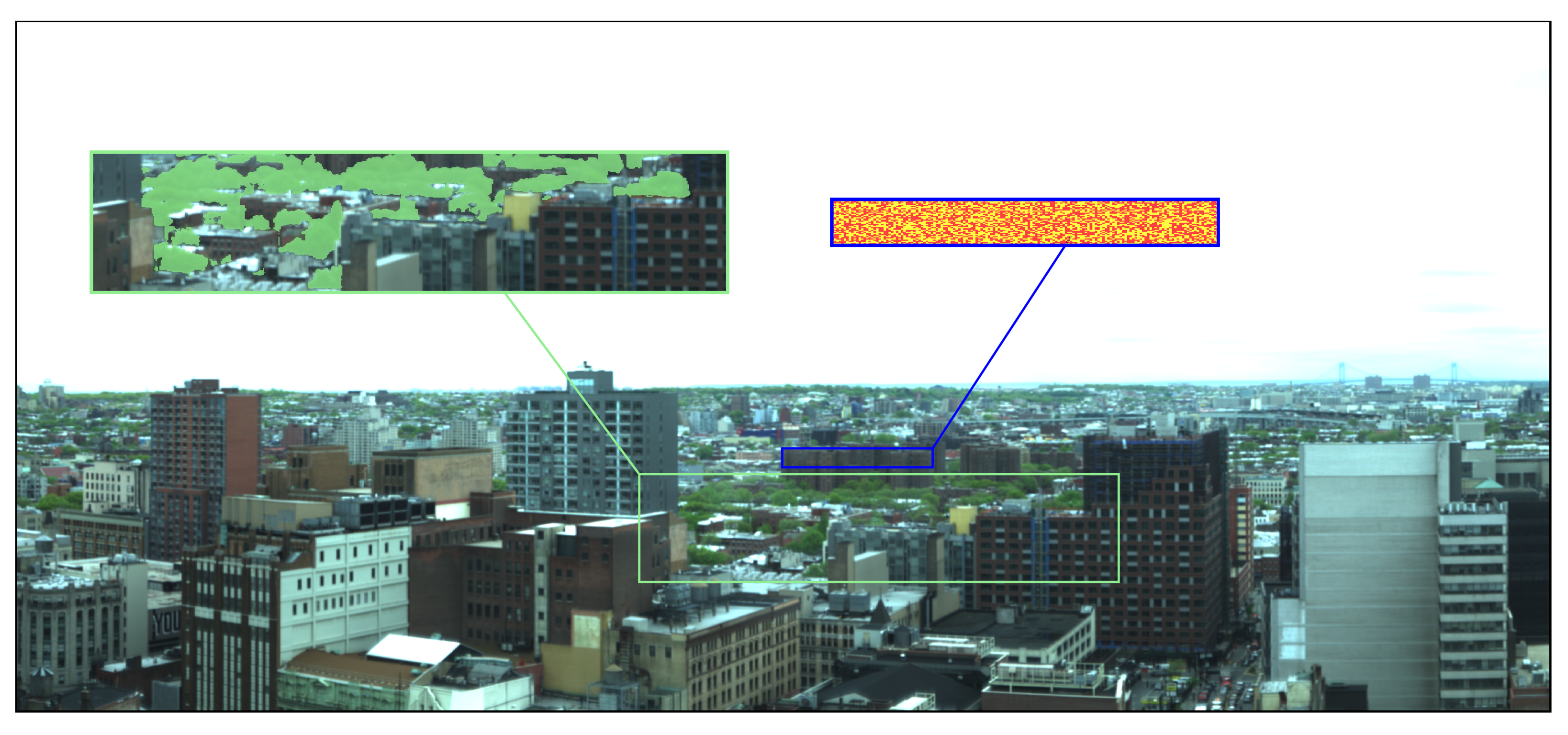
In this work, we use a simple
k-means clustering of pixel spectra to segment an image that had optimal uniform lighting and minimal shadowing into 10 clusters (we show below that the distinct nature of vegetation spectra results in performance that is comparable to more complex machine learning algorithms [
77]). The resulting label map of the
k-means clustering is shown in
Figure 2 together with the mean spectra of pixels in the 10 clusters. The spectra of clusters 2 and 5 show the uniquely identifying features of vegetation; namely, the enhanced chlorophyll and leaf pigment reflectivity in the visible green peak range of ~0.5–0.6 μm, absorption in the red range of ~0.6–0.7 μm, the red edge at ~0.7 μm, and high reflectance in near-IR due to spongy mesophyll in the plants’ cellular structure. The green box in
Figure 1 has an overlay of the pixels labeled as 2 and 5 by
k-means in green to qualitatively show the accuracy of the unsupervised labeling. To demonstrate the robustness of this simple method for selection of vegetation pixels, we compare its performance with that of the 1D-CNN described in [
74] for the scene in
Figure 2. The performance of supervised machine learning models is often evaluated using “precision” and “recall”. For a set of objects with known classifications, precision represents the fraction of classification predictions for which the model was correct, while recall represents the fraction of all instances of a given class that were correctly predicted by the model. Overall, while the CNN was far superior in identifying the various human-built and natural materials in the urban scene, both the CNN and
k-means showed identical performance metrics for labeling
vegetation pixels (precision = 1.00, recall = 0.98), with the mean vegetation spectra from both methods differing by <4% overall.
We note that the selection of vegetation pixels is not carried out for each HSI scan separately, but rather the pixels selected in
Figure 2 are used in all scans in the observational campaign. This is justified by the fact that our HSI instrument is immobile and constantly observing the same scene, with pixel-level accuracy in the instrument pointing over the period of this study. Therefore, the pixels containing vegetation remain constant over all obtained images. Thus, the classification task need only be implemented once to label the pixels as either vegetation or non-vegetation before applying that labeling to all. Furthermore, as shown in [
74], the same scene under less optimal lighting and cloud conditions can result in a measurable difference in classification accuracy. Repeating the
k-means clustering for two other scans, one in the morning (08h31) and one in the afternoon (18h01) where both exhibit significant shadowing, the precision of the clustering of vegetation pixels remained at 1.00, however, the recall dropped to 0.70 and 0.68, respectively. Since the accuracy of identification is variable while the pixels containing vegetation are constant across images, a single image taken at midday with optimal lighting and cloud conditions was chosen for segmentation.
2.2. Compound Ratio
In daytime hyperspectral imaging at Visible and Near-Infrared (VNIR) wavelengths of 0.4–1.0 μm, atmospheric interactions with solar radiation result in significant modifications to the spectrum received by the sensor as the light travels from the top of the atmosphere to the imaged object, and from the object to the sensor. Assuming emissions and surface reflectance are Lambertian [
78], the geometric series expression for the radiance reaching the sensor (
) at wavelength
and time
t can be expressed as:
where
is the surface reflectance,
is the total outward atmospheric transmission between the target and the sensor, and
is the total irradiance incident on the target, which is the contribution of solar irradiance and downward atmospheric transmission from the top of the atmosphere to the target. In the particular case of vegetation, due to plant fluorescence under solar illumination, there is an added weak emission with a magnitude of 2–5% of the reflected radiation in the near-infrared. This fluorescence (
) is added as a perturbation to Equation (
1) such that the radiance reaching the sensor from vegetation becomes a composition of two coupled contributions, the reflected (
) and the emitted (
) light:
With spectroscopic measurements of vegetation health via remote sensing, it is common to compute the apparent reflectance (
), which is the ratio between upwelling and incident fluxes, and accounts for the solar-induced fluorescence emission normalized by the irradiance incident on the target at surface level [
78,
79]:
In order to obtain this apparent surface reflectance, it is imperative to account for and remove the effects of the atmosphere from the spectrum. Unlike satellite and aerial imaging, due to the orientation of ground-based HSI, the amount of atmosphere that light traverses prior to reaching the sensor varies significantly for each pixel. Therefore, correcting for atmospheric effects requires knowledge of observing geometries such as zenith and azimuth angles, sensor field of view, location of the Sun, and distance to each pixel, as well as atmospheric conditions and compositions, which may vary between the areas closer to the sensor and those at the horizon. Radiative transfer codes are commonly used in remote sensing applications to correct for atmospheric effects by modeling attenuation using assumed atmospheric conditions and concentrations and extracting surface reflectivity from the measured intensity by the sensor [
80,
81,
82]. However, due to the oblique geometry of proximal remote sensing, the determination of the incident spectra is extremely difficult. In addition, given the varying distances of objects across the image from the sensor and the associated differences in atmospheric conditions across the image, atmospheric corrections with simulations of atmospheric effects can vary significantly across the image.
Therefore, in lieu of modeling the atmospheric effects, here we propose the use of a “
Compound Ratio” for the analysis of vegetation spectra in urban environments that uses time-dependent comparisons of vegetation spectra with a nearby built structure to isolate the changes in vegetation apparent reflectance. In
Figure 1, all the vegetation pixels inside the green rectangle are at an approximately uniform distance from the sensor. The buildings in the blue rectangle are at roughly the same location as the vegetation. Therefore, utilizing Equations (
1) and (
2), the mean at-sensor signal of the vegetation and building pixels can be expressed as:
where
and
are the mean measured intensity of the vegetation and buildings (respectively) at wavelength
and time
t. By considering the following assumptions:
buildings have constant reflectivity over time, ,
the total irradiance incident on the target is identical for buildings and vegetation, ,
atmospheric transmission is identical for buildings and vegetation, .
Normalizing the intensities of each scan at
t by the measured value at the start of the observing campaign
results in
where the last equality follows from assumption 1 above and we have dropped the
V and
B superscripts on
and
due to assumptions 2 and 3 above. Dividing the normalized intensities of vegetation in Equation (
6) by those of the buildings in Equation (7), we isolate the
relative change in the apparent reflectance of vegetation over time by defining the
Compound Ratio of vegetation
:
It is important to note that vegetation reflectance is affected by the angle of the incoming spectrum due to factors that include leaf orientation and sun-sensor geometry [
83,
84]. However, the formulation above implicitly assumes that reflectance is independent of the angle of incoming radiation. While this may result in residuals that can impact the accuracy of the Compound Ratio, integrating the spectrum of vegetation over the entire canopy within the green box in
Figure 1 minimizes this effect. To provide a control sample demonstrating the soundness of the Compound Ratio assumptions, the pixels of the buildings in the blue box in
Figure 1 were randomly split into the two sets represented by the red and yellow labels shown. This allows us to calculate both the Compound Ratio of vegetation-to-buildings (
) from Equation (
8) using one set of building pixels, as well as the Compound Ratio of buildings-to-buildings (
) using the two sets of randomly split building pixels. If all the assumptions listed above hold true, it is then expected that the Compound Ratio of buildings-to-buildings should result in a constant value of 1 in both wavelength and time dimensions. Furthermore, as seen in
Figure 2 the building used for the control is composed of several human-built materials with slightly different spectra. By randomly splitting the building pixels into two sets, we minimize the allocation of any one single material to each set and maximize the likelihood that the Compound Ratio of building-to-building would capture the changes in apparent reflectance of the building rather than the change in one particular spectrum of one material relative to another.
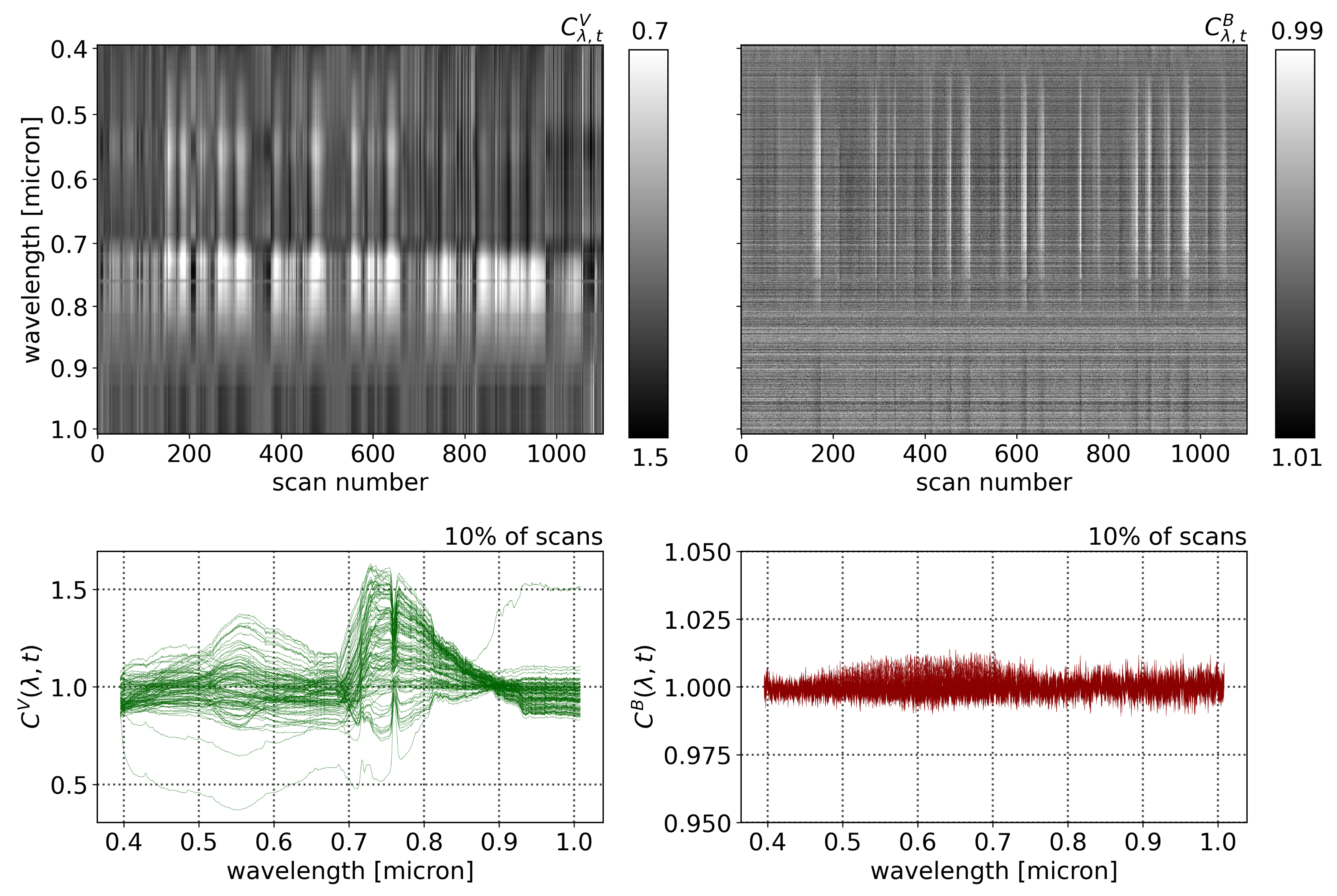
Figure 3 shows a mapping of the Compound Ratios of vegetation and buildings for all wavelengths and scans in the top row, while the bottom row shows the Compound Ratios of 10% of scans, randomly selected and plotted as functions of wavelengths. Noting the difference in scaling of the color-bars in each mapping as well as the y-axis of the bottom plots, it is evident that the assumption of lack of reflectivity holds true for buildings as the amplitude of change in Compound Ratios of buildings is dominated by noise that is varying at the ~1% level. On the other hand, the Compound Ratio of vegetation shows
variation over time in the green peak of chlorophyll, the red edge, absorption in red, and emission in near-infrared, all unique identifiers of the vegetation spectrum. These variations reach the ~50% level, which is in line with previous studies [
85,
86]. Thus, we find that the plant reflectivity itself is changing on 15 min time scales.
It is worth noting that in the Compound Ratios of vegetation in
Figure 3, there is visible absorption occurring at wavelengths ~0.76–0.77 μm. The instrument used in this work does not exhibit sharp wavelength-dependent sensitivity that would cause such a feature. Therefore, it is likely to result from residual A-band absorption of oxygen in the atmosphere. The presence of atmospheric absorption following the previously mentioned treatment to remove atmospheric effects is indicative that the assumptions may not be absolute. Dirt, moss, and sticking of pollutants to the surfaces of buildings affect assumption 1. Furthermore, assumptions 2 and 3 require that the vegetation and comparison buildings are at the exact same location, thus, any deviation can cause the depth of the atmosphere as well as amount of incident light to differ between the two objects and result in residual atmospheric effects in the final Compound Ratio. Moreover, the Compound Ratio of buildings in
Figure 3 shows small illumination variations in the visible portion of the spectrum from ~0.45–0.7 μm that resemble the residual from the solar spectrum. However, given the small magnitude of changes in building Compound Ratios we can be confident that changes seen in the Compound Ratios of vegetation are far more likely to be due to changes in vegetation reflectivity rather than atmospheric effects, especially considering that the varying features are all characteristic of vegetation spectra. Further investigation into the soundness of using the building as atmospheric irradiance and transmission control for the vegetation is presented in
Appendix B.
2.3. Air Quality Measurements
For the purpose of this work, we use measurements of O
3 and PM
2.5 concentrations, temperatures, and humidity (air moisture content). We use temperatures and relative humidity measurements from available Weather Underground data (
https://www.wunderground.com/, accessed on 6 June 2016) for the location, days, and times of our HSI scans. Relative humidity was then converted to absolute humidity (mass of water vapor per unit volume of air, g/cm
3) using the general law of perfect gases, the specific gas constant for water vapor, and assuming 1 atm pressure. For the O
3 and PM
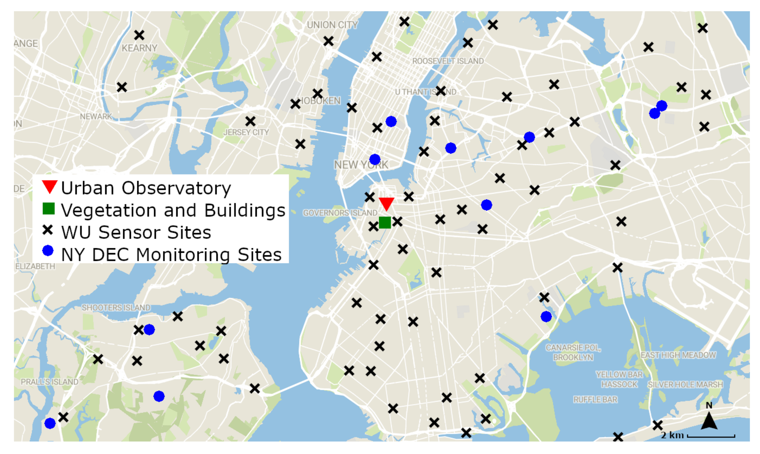
2.5 concentrations at the times of our scans, we use the openly available New York State Department of Environmental Conservation (NYS DEC) data. The locations of the NY DEC’s air quality monitoring sites, and the approximate locations of the Weather Underground crowdsourced network of air quality sensors, are shown in
Figure 4 together with the location of the vegetation and buildings used in this study, and a summary of the data obtained from each source is shown in
Table 1. For obtaining the individual air quality measures used in this study for each scan, we took the average O
3, PM
2.5, temperature, and humidity at each scan time over a large area, including outside the near vicinity of our selected vegetation and buildings. Although the sensor network is distributed over a large area and not directly adjacent to the vegetation patch under study, we take the average values for several reasons. It is well known that individual air quality sensors require precise and periodic calibration and tend to be noisy [
87,
88], especially in the presence of the urban island heat effect and localized emissions in urban environments [
89,
90]. Although calibration of the sensor network is outside the scope of this paper, averaging multiple measurements from different sensors can reduce the impact of noise on the individual measurement. Furthermore, as evident in
Figure 4, there are no air quality monitoring sites directly atop or adjacent to our imaged vegetation and buildings. Averaging the surrounding measurements allows us to extract a relatively accurate representation of the air quality values of our given location.
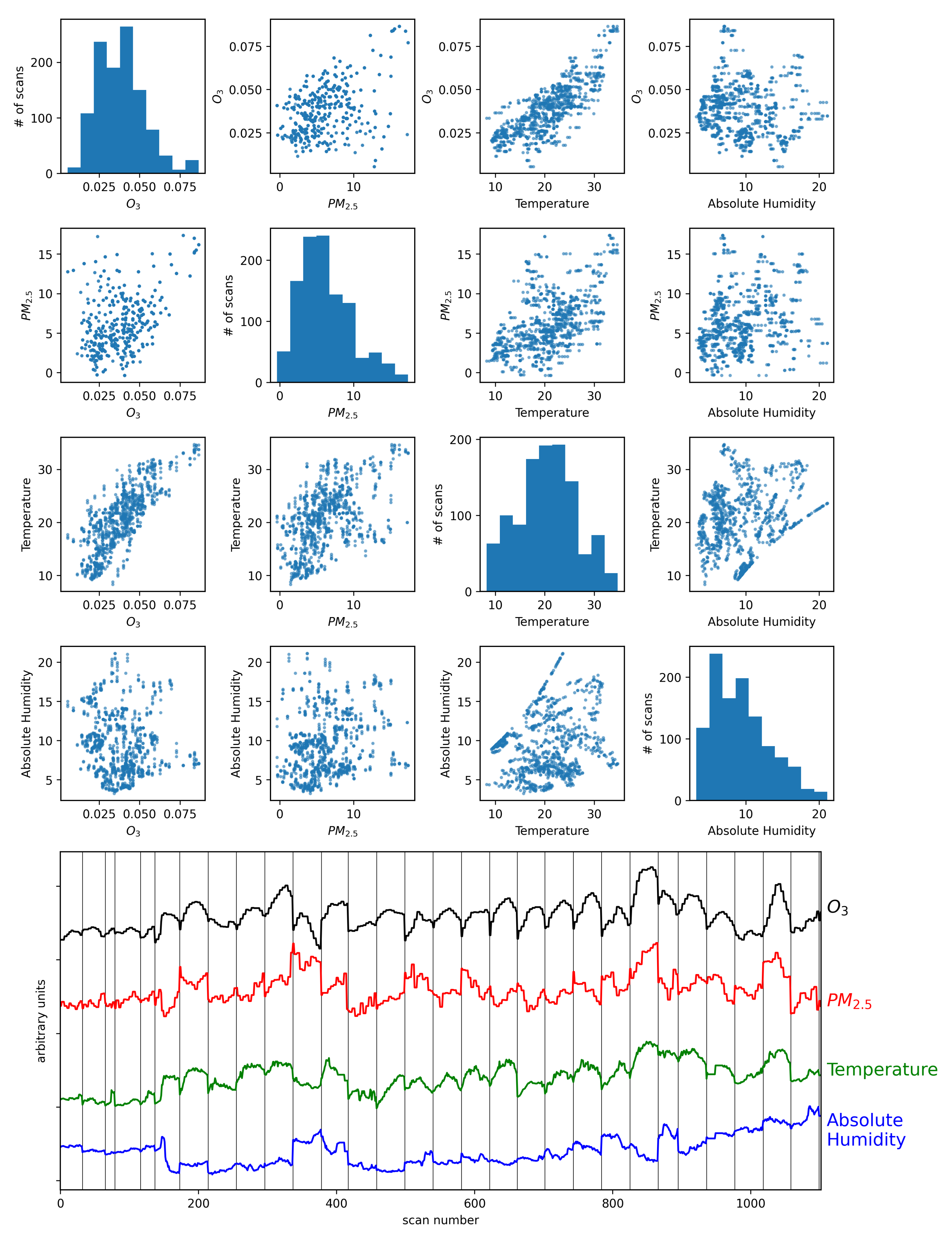
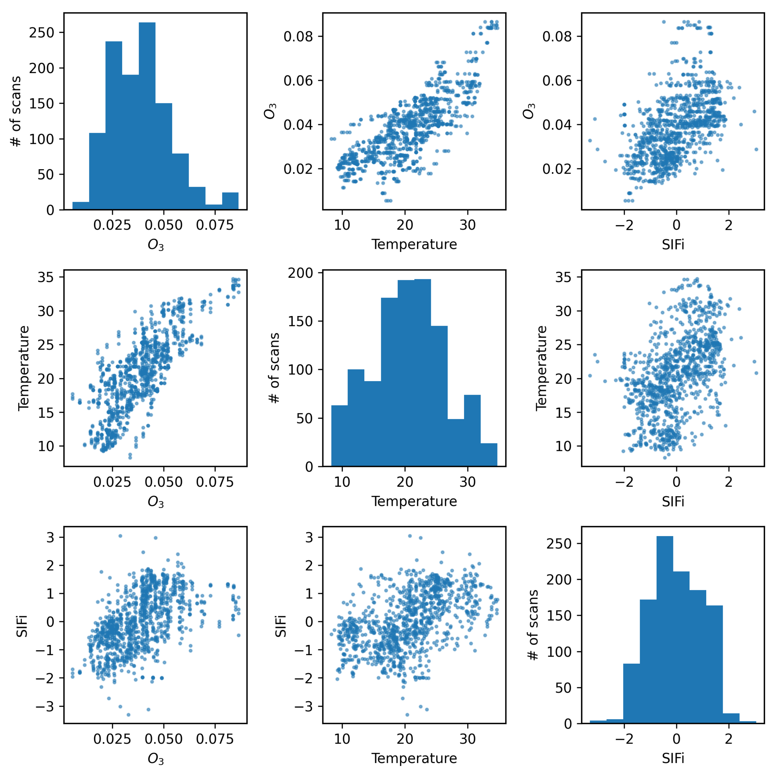
Figure 5 shows the four air quality parameters for each scan time in a scatter matrix (scan times with precipitation or 100% relative humidity were removed from the sample to eliminate any effects of rain drops near the camera). It is worth noting that there is a visible correlation between ozone and temperature. The figure also shows the four air quality parameters after standardization (
,
) plotted as functions of scan number, where it is further evident that O
3 and temperature exhibit correlated changes with time. Studies over multiple time scales have shown that there is a strong correlation between surface temperature and O
3 concentrations [
34,
35,
36], with temperatures having a correlation coefficient up to ~80% when used to estimate ozone concentrations in urban environments [
91]. This correlation becomes more complex with PM
2.5 where studies have shown that a positive correlation between PM
2.5 and O
3 exists at high temperatures, and a negative correlation at lower temperatures [
92]. Furthermore, temperature inversion and the mixing of atmospheric layers can have a significant impact on O
3 and PM
2.5 concentrations as well as humidity [
37,
38], which adds further complexity to their correlations and covariances.
2.4. Tracers of Vegetation Health
The concept of utilizing the leaf optical responses to study the impact of various stresses on vegetation health has been used widely in the remote sensing field [
59,
93,
94]. The justification behind using the spectral wavebands from 400–2500 nm as predictors of plant health is that unfavorable conditions result in morphological and physiological changes in plants that disturb the processes of transpiration and photosynthesis and, therefore, impact the manner with which the plants interact with light. The part of the spectrum in the visible wavelengths from 400–700 nm is primarily influenced by colored pigments such as chlorophyll and carotenoids [
95,
96,
97], while the 700–1400 nm range reflects leaf structural characteristics [
98], and 1400–2500 nm is mainly affected by the tissue water content [
99]. Due to the central role of chlorophyll in the process of photosynthesis, chlorophyll content is often used as an indicator for plant physiological health [
100,
101]. Aside from chlorophyll, carotenoids, including
- and
-carotenes and xanthophylls, are the other main pigments of green leaves with particular physiological functions related to photosynthesis. Visually, reductions in chlorophyll are perceived as yellowing of leaves primarily due to the relative increase in carotenoid content [
102], which are retained during leaf senescence as a mechanism of photoprotection. Therefore, changes to carotenoid content and their proportion to chlorophyll content are also widely used as indicators of physiological and health status in plants [
96,
103]. Other common indicators of physiological and morphological changes detectable in the spectra of vegetation and used as cues for changes in plant health include leaf dry matter content, also known as leaf mass [
99,
104], leaf water equivalent layer [
105,
106], and leaf senescence [
61,
107].
The Soil Canopy Observation of Photosynthesis and Energy fluxes (SCOPE) model couples photosynthetic, hydrological, and radiative transfer models to provide simulations of hyperspectral radiance and net radiation, photosynthesis rates, and various heat fluxes for soil, leaves, and vegetation canopies [
108,
109]. Using SCOPE to simulate the apparent reflectance of vegetation with varying morphological and physiological properties allows for the demonstration of the aspects of the proposed Compound Ratio that correspond to tracers of vegetation health. Vegetation with varying chlorophyll AB content (
), carotenoid content (
), dry matter content (
), leaf water equivalent layer (
), and senescent material fraction (
) has spectra that reflect different health statuses.
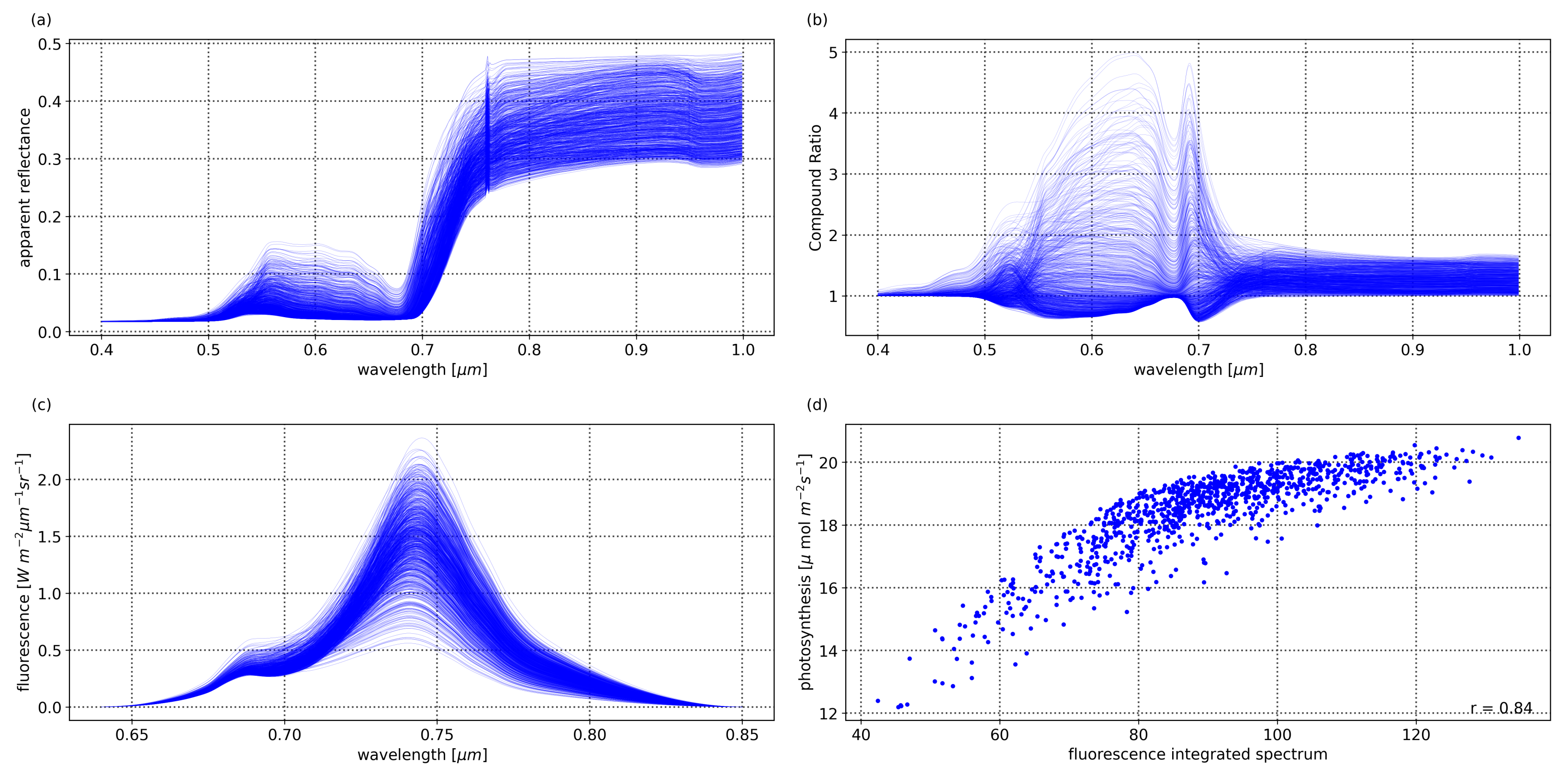
Figure 6a shows the SCOPE simulations of the apparent reflectance (
)—which includes the fraction of radiation in the observation direction (
R) with the added ratio of emitted fluorescence to irradiance (
)—produced by varying the aforementioned indicators of physiological and health status in plants. The ability to utilize the spectra of vegetation to extract information regarding their health is exemplified by the significant changes in the simulated spectra when varying their physiological and morphological status indicators. The Compound Ratio as presented in
Section 2.2 is essentially the rate of change in apparent reflectance.
Figure 6b shows the Compound Ratio computed for the simulated apparent reflectances by considering one of the simulations as being
(the apparent reflectance at time
) to use as the denominator of Equation (
8), which demonstrates the ability of the proposed Compound Ratio to reflect the changes in the health status of vegetation.
For this work, we rely on two methods for quantifying vegetation health from its Compound Ratio spectra: a simple ratio of the wavelength where solar-induced fluorescence peaks relative to a control wavelength, and the amplitudes of a Principal Component Analysis (PCA) decomposition that captures variation in the entire spectrum of a given scan.
2.4.1. Solar-Induced Fluorescence (SIF)
Solar-Induced chlorophyll Fluorescence (SIF) has a functional connection with photosynthesis and an insensitivity to atmospheric scattering, and has therefore been proven to be an effective signal for monitoring vegetation physiology with significant advantages over other remote sensing indicators [
110,
111]. Photosynthetically active energy absorbed by vegetation can be used in photochemical reactions, re-emitted as fluorescence, or dissipated as heat, and any efficiency change in one of these processes results in alterations in the remaining two. Therefore, unlike commonly used indices that rely on reflectance-based parameters such as the Normalized Difference Vegetation Index (NDVI) or the Photochemical Reflectance Index (PRI), SIF is a byproduct of photosynthesis and an indicator of Gross Primary Production (GPP) [
112,
113]. Since SIF contains information on Photosynthetically Active Radiation (PAR), it has been used as a strong indicator for photosynthesis, and gives a measure of plant stress responses to changes in temperature, water availability, nutrients, and other environmental and health factors [
114,
115].
Figure 6c shows the SIF spectrum for the SCOPE simulated vegetation spectra with varying levels of
,
,
,
, and
which reflect the ability to infer the health of the plants from the changes in the levels of SIF. Furthermore, by integrating the fluorescence spectra to obtain the area under the SIF curve,
Figure 6d shows the strong correlation between solar-induced fluorescence and photosynthesis rates in vegetation with a Pearson’s correlation coefficient of 0.84.
There are two major methods with which SIF is quantified: radiance-based and reflectance-based methods. Radiance-based methods depend primarily on exploiting the narrow absorption feature of the Fraunhofer line for telluric oxygen (O
2A) at 760.4 nm to isolate SIF from the reflected spectrum, which allows for the estimation of SIF in physical radiance units if the data are calibrated. The majority of radiance-based methods in the literature essentially derive from the Fraunhofer Line Depth (FLD) principle, initially proposed by [
116,
117]. The FLD method relies on two measurements of the radiance, one inside and one outside the O
2 Fraunhofer absorption bands, where the magnitude of SIF is computed by comparing the magnitude of the measured signals. In essence, FLD methods require knowledge of the incident solar irradiance (
E in Equation (
2)) and target radiance (
L in Equation (
2)) at wavelengths in the bottom and shoulder of the absorption feature in order to solve for the magnitude of fluorescence under the assumption that Reflectance (
R) and Fluorescence (
F) are constant at the two wavelengths. Refinements and enhancements to this method have been introduced, including the three-channel FLD (3FLD) [
118], FLD with correction factors (cFLD) [
119], and improved FLD (iFLD) [
120], all of which follow the same principle with modifications. More sophisticated methods for retrieving the full SIF spectrum generally rely on either Spectral Fitting Methods (SFMs) which do not rely on the assumption of constant reflectance and fluorescence such as the Fluorescence Spectrum Reconstruction (FSR) [
121], or model inversion approaches [
122].
Reflectance-based methods, on the other hand, rely on the effects of fluorescence on the apparent reflectance spectrum in the red-edge region rather than the Fraunhofer line. While radiance-based approaches generally produce measurements of fluorescence with physical units, reflectance-based methods rely on computing indices that actually reflect vegetation physiological changes that are strongly correlated with the same processes responsible for changes in fluorescence (as opposed to tracking the fluorescence emissions themselves). Since SIF extends over the wavelength range of 640 to 850 nm, with a broad peak centered at 750 nm and a smaller peak near 690 nm [
123], these indices are computed using the apparent reflectance at a wavelength affected by fluorescence (typically around one of the two fluorescence maxima at 690 and 750 nm) compared to another that is less or not affected by fluorescence. Some examples of the use of reflectance-based indices include
,
,
,
, and
, as well as curvature indices such as
[
123,
124,
125,
126,
127,
128,
129]. While a full decoupling of the fluorescence effects from the apparent reflectance cannot be achieved using these methods, the normalization of the reflectance using ratios optimizes the indices that are sensitive to changes in fluorescence and have an advantage over radiance-based approaches by not requiring complex processing and knowledge of various fluxes and parameters.
As shown in
Section 2.2, the Compound Ratio is computed in our data from the radiance received at the sensor in order to isolate the changes in apparent reflectance of vegetation from the atmospheric transmission and incident irradiance on the target. In
Figure 3, changes in the Compound Ratio at wavelength ~0.75 μm can visibly be matched with concurrent changes in air quality parameters for similar scans in
Figure 5. On the other hand, the Compound Ratio at wavelengths of 0.9 μm presents relatively little to no variation with time. Given these observations, and the fact that the Compound Ratio is a measure of the change in reflectance rather than radiance, we employ a reflectance-based approach and measure the variation in fluorescent emissions by using a Solar-Induced Fluorescence indicator (
) computed as a simple ratio of the amplitude of the Compound Ratio at 0.75 μm relative to that of the less affected reference at 0.9 μm as:
Using the SCOPE simulated spectra in
Figure 6, the SIF indicator was calculated using Equation (
9), with the values shown for various parameter values in
Figure 7. Provided that the Compound Ratio is the relative change in reflectance, we also compute the relative change in the various vegetation parameters from the output of SCOPE (
, such that
x is
for chlorophyll AB content,
for carotentoid content, etc.) by considering one simulation to be the parameter at time 0, and computing the change in each
in the same manner shown in Equation (
8). In
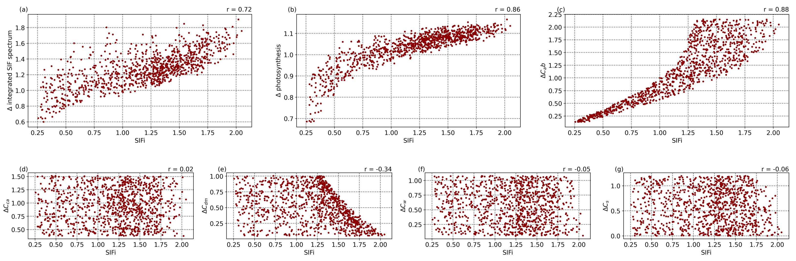
Figure 7a, there is a clear correlation between the SIF indicator and the change in fluorescence quantified by integrating the simulated fluorescence spectra in
Figure 6c with a Pearson’s correlation coefficient (
r) of 0.72. Given the input parameter values, it is evident that these correlations are primarily driven by changes in chlorophyll AB content (
), with a weaker influence by dry matter content (
) and relatively no impact from carotenoid content, leaf water equivalent layer, or senescent material fraction. Given the relation between fluorescence and photosynthesis rate as seen in
Figure 6d, this correlation also translates into a strong correlation between the SIF indicator and the change in photosynthetic rate seen in
Figure 7b (
) and shows that it is reasonable to use this indicator as a tracer of vegetation health.
2.4.2. Principal Component Analysis (PCA)
Vegetation indices that use linear or ratio combinations of various wavelengths selectively indicate stress conditions in a particular domain; for example, indices based on the red edge such as NDVI and RDVI [
130] represent a measure of leaf chlorophyll content, while xanthophyll-related indices such as PRI focus on the green peak. However, the full vegetation spectrum from 0.4–1.0 μm contains information on pigments, cellular biochemicals (proteins, lignin, cellulose), and water leaf content, among various other indicators of plant health. Therefore, hyperspectral imaging provides a wealth of information on the status of vegetation throughout the VNIR wavelength range. Using the entire spectrum rather than a few narrow bands has the potential to offer a more holistic approach to capturing the health of vegetation. On the other hand, hyperspectral images are known to contain redundant information, and so Principal Component Analysis (PCA) decomposition is commonly used in hyperspectral analyses to reduce dimensionality by removing such redundant information while encoding global spectral information important for identifying vegetation health in a set of characteristic spectra [
131,
132]. In our case, PCA uses correlated spectral attributes of the Compound Ratio spectra at the various time steps to determine an orthogonal basis set of
N Principal Component (PC) spectra that describe the principal variability in them. Using
results in principal components that explain a total of >99% of the variability in the vegetation’s Compound Ratio spectra, and any additional components yield relatively insignificant explained variances (<0.5%).
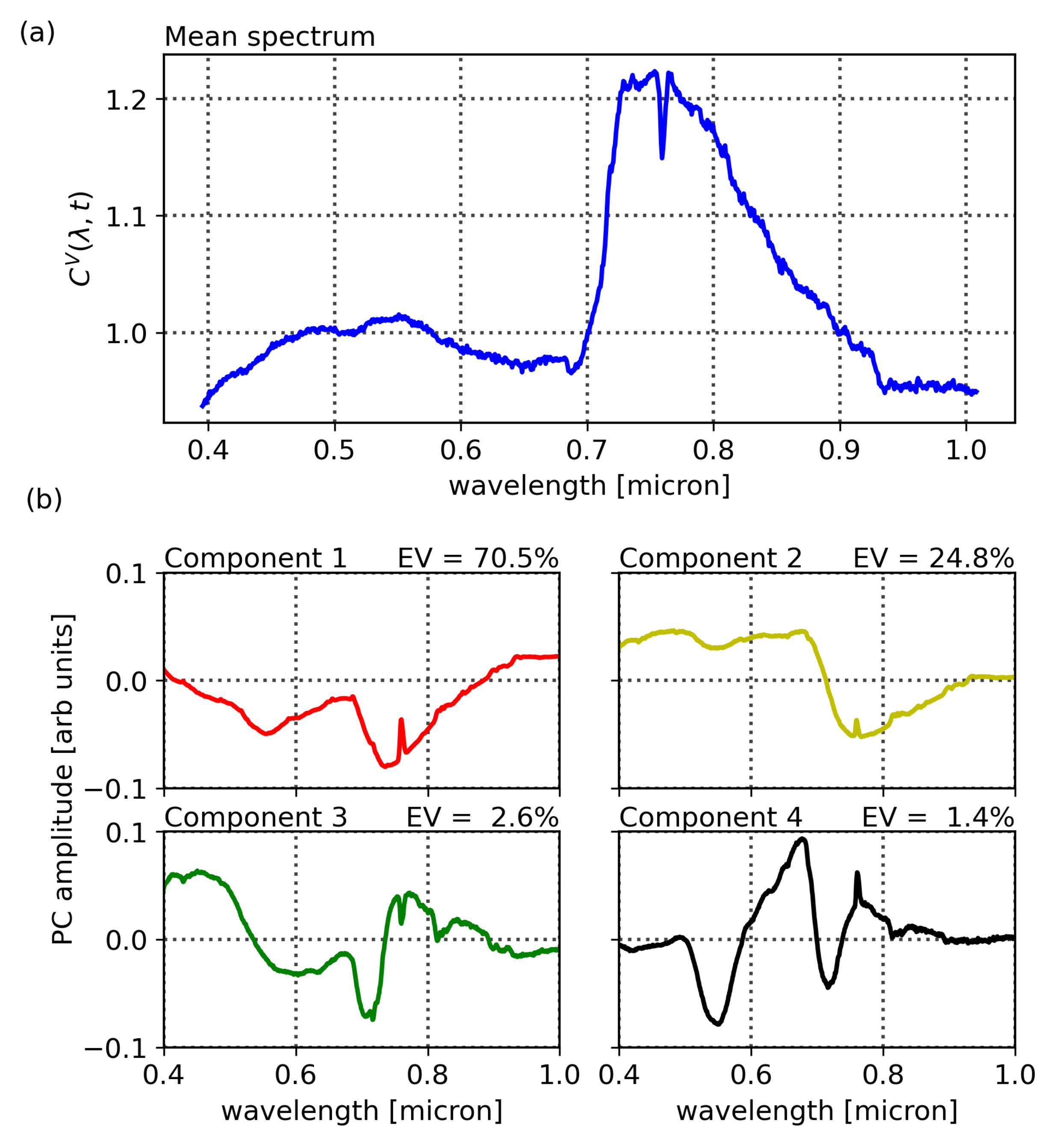
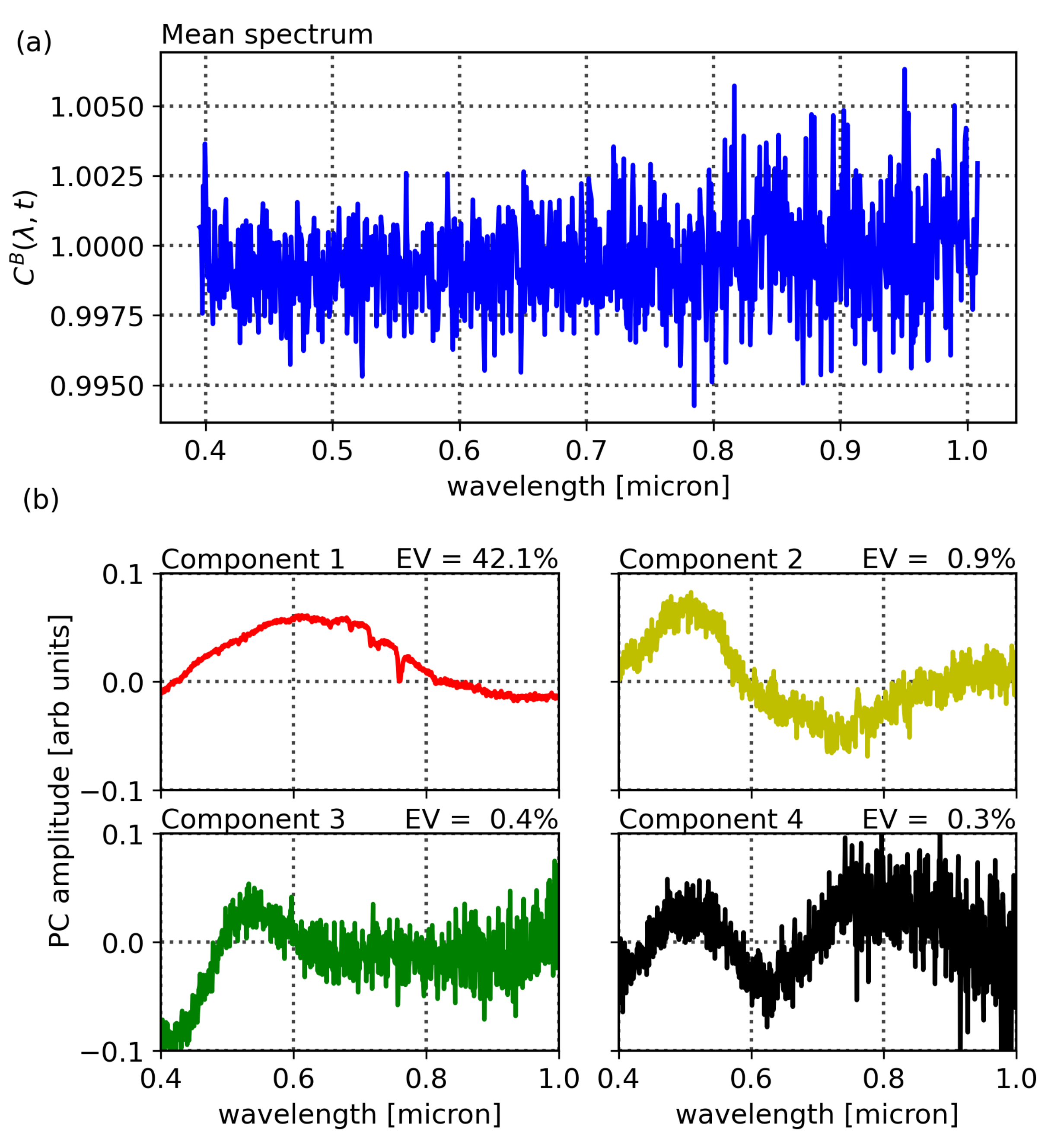
Figure 8 and
Figure 9 show the PCA decomposition of the vegetation and building spectra, respectively, where the explained variances for the components in vegetation are 70.5%, 24.8%, 2.6%, and 1.4%, while those of the buildings are 42.1%, 0.9%, 0.4%, and 0.3%. We note that their shapes clearly show the dominance of noise in the composition of the spectrum of buildings.
Dimensionality is reduced by projecting each 848-channel Compound Ratio spectrum onto the
N components and, as we describe in
Section 3.2, it is the variability in those projected amplitudes that is compared with air quality variability. This variability in amplitudes in essence is a measure of the variations in vegetation spectra, and given that changes in the health of vegetation result in variations in their spectra proportional in magnitude to changes in health status, it follows that the variability in projected amplitudes is representative of vegetation health. To test this claim, we performed the same PCA decomposition on the Compound Ratio spectra calculated from the SCOPE simulated apparent reflectances in
Figure 6. In the same manner as in
Section 2.4.1, we explore the correlation between the various principal component amplitudes and the parameters of the model and show their correlation coefficients in
Table 2. Principal component 1 shows a significant inverse correlation with the change in the rate of photosynthesis (
) and the chlorophyll AB content (
). Principal component 2 exhibits a weaker correlation with photosynthesis rate (
), but shows a significant inverse correlation with dry matter content (
). Principal component 3 shows levels of correlation with photosynthesis (
), chlorophyll AB content (
), dry matter content (
), and senescent material fraction (
), but it also exhibits stronger correlation with carotenoid content (
). Lastly, component 4 shows only a weak correlation with chlorophyll AB content (
), and stronger correlation with carotenoid content (
).
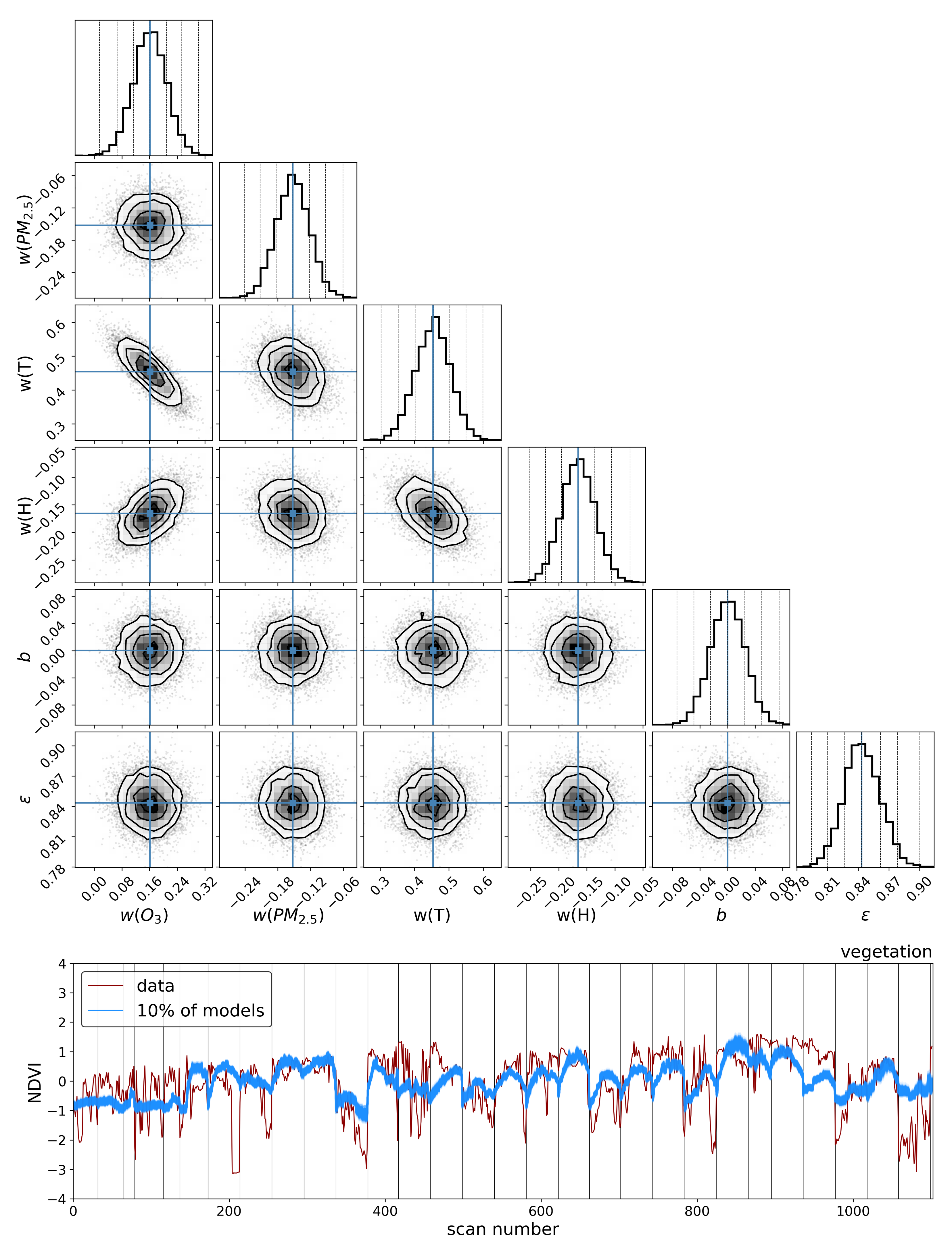
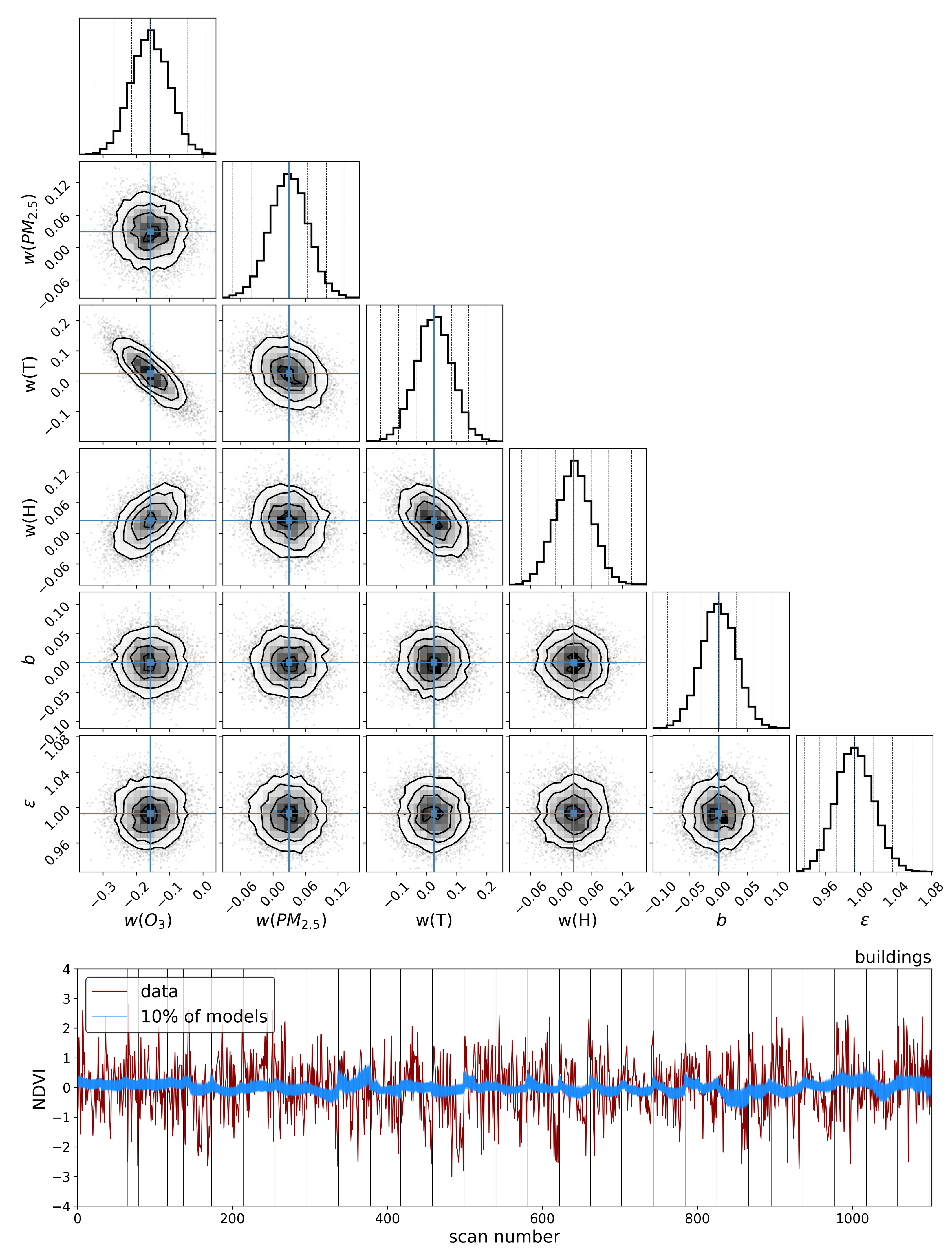
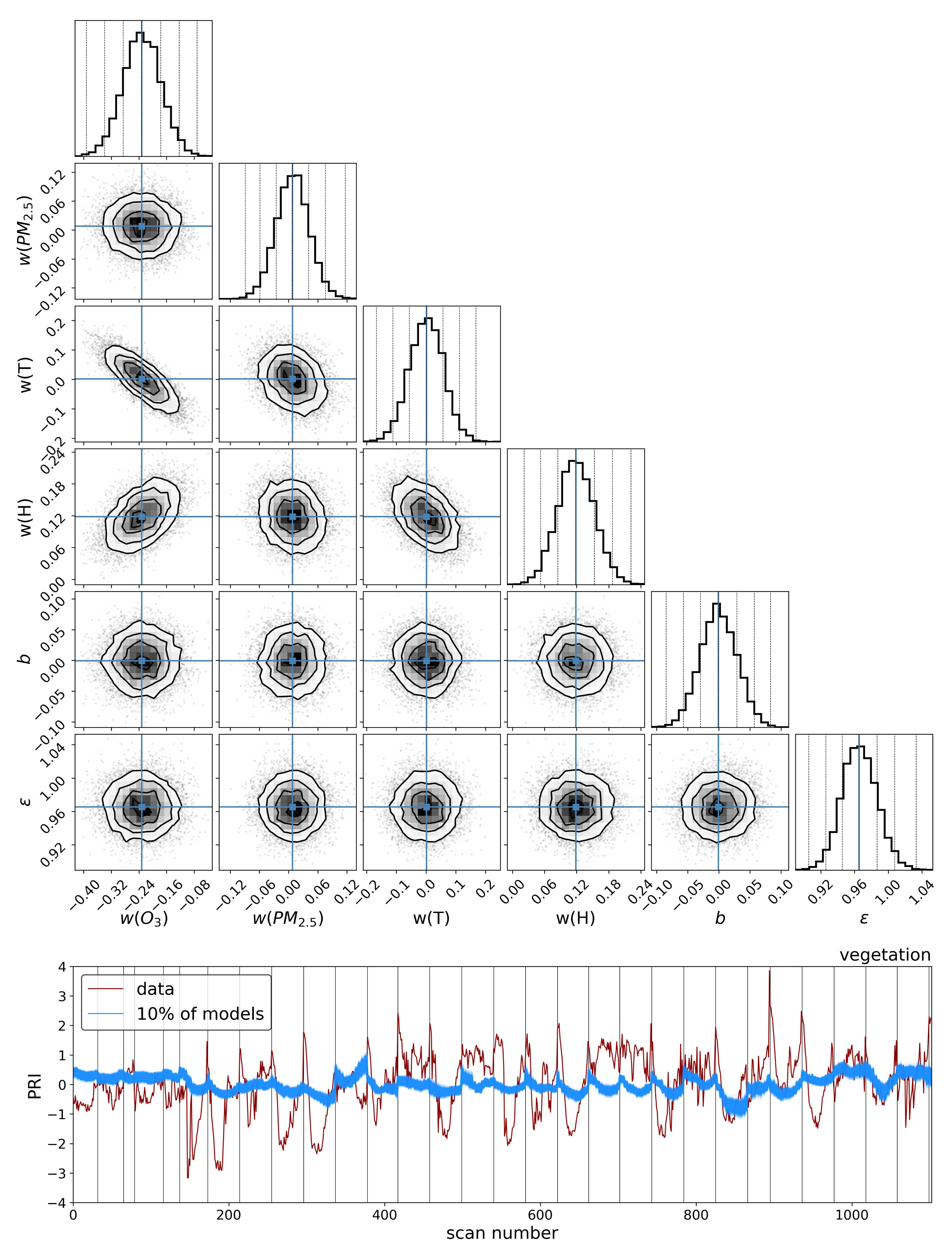
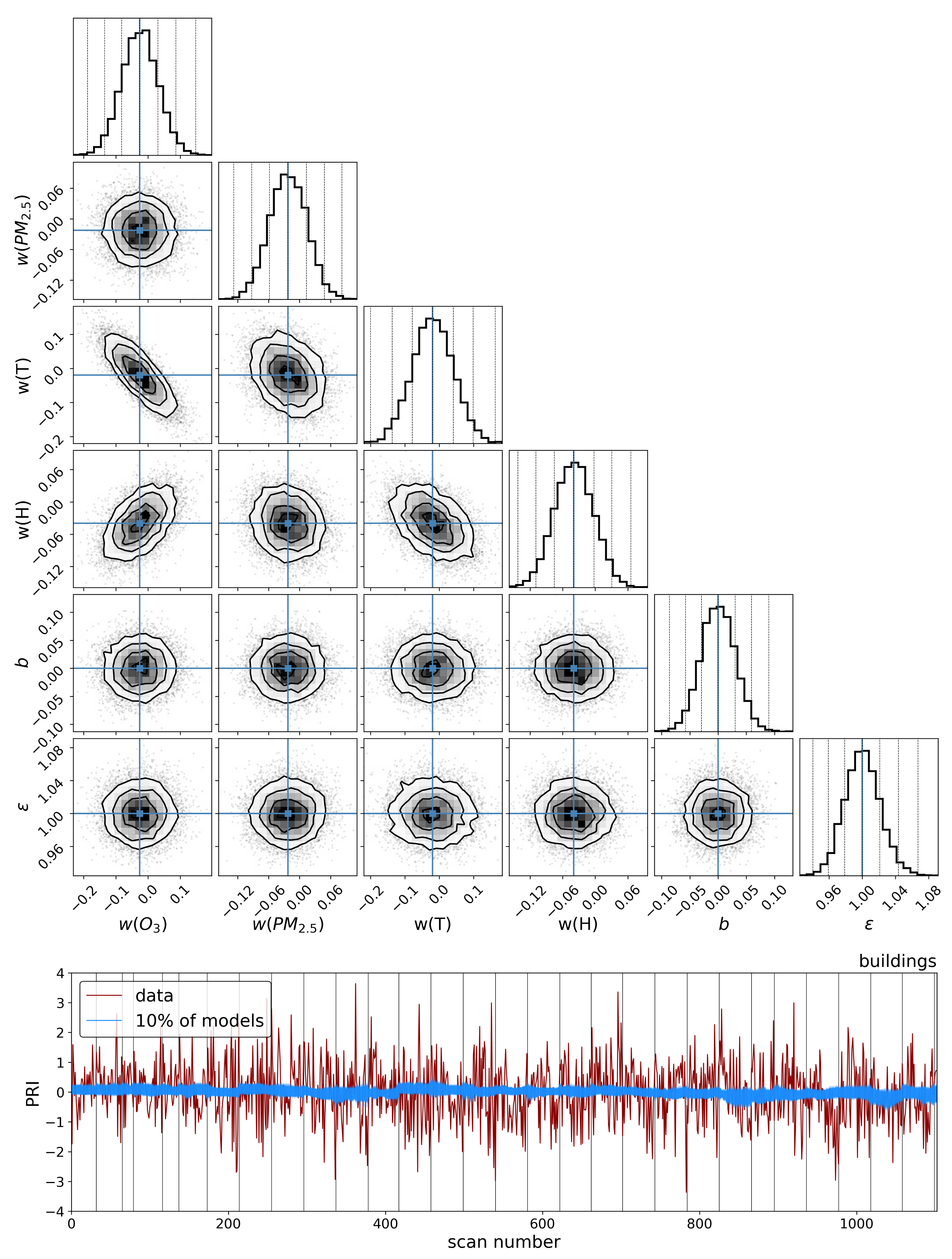
2.4.3. Linear Model
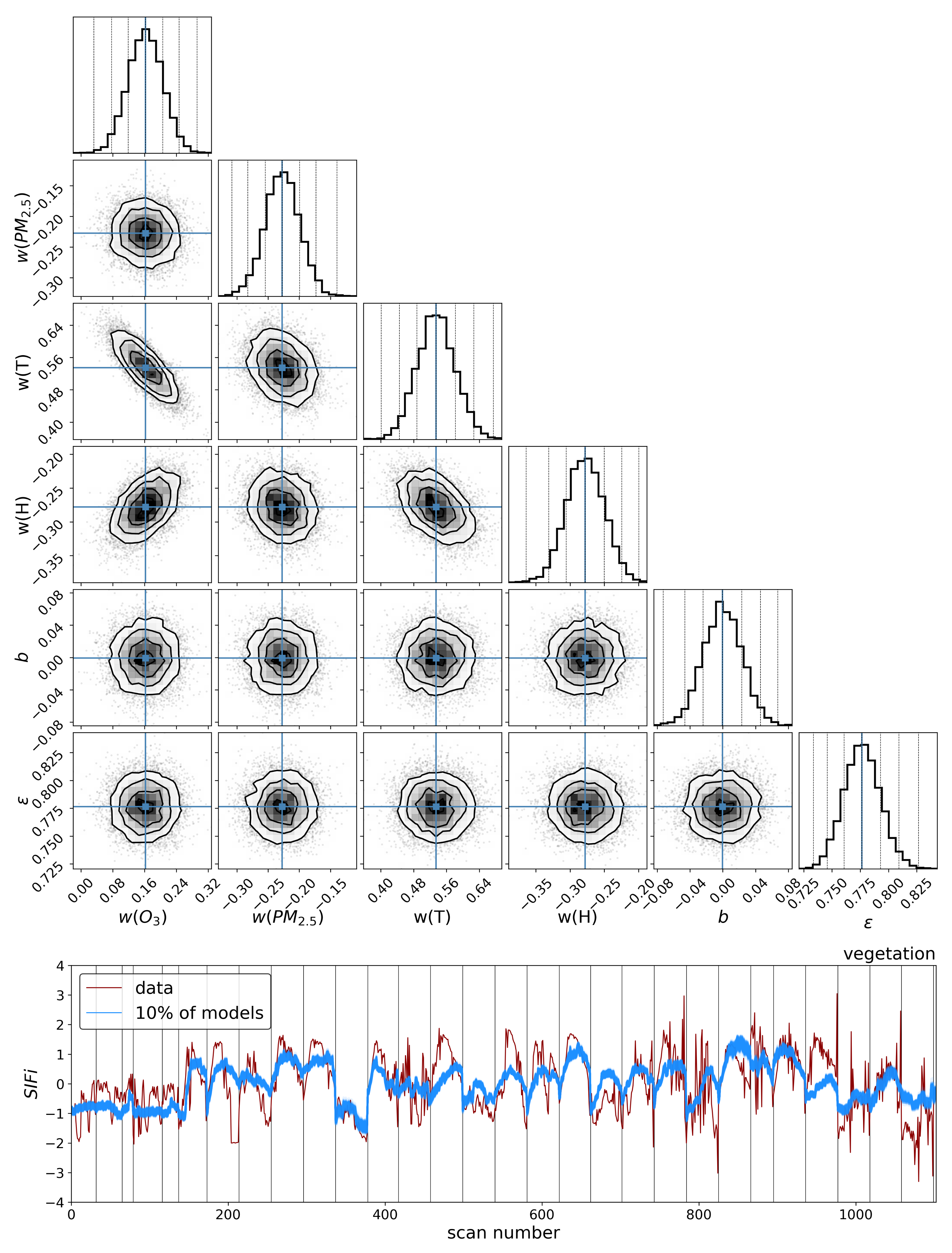
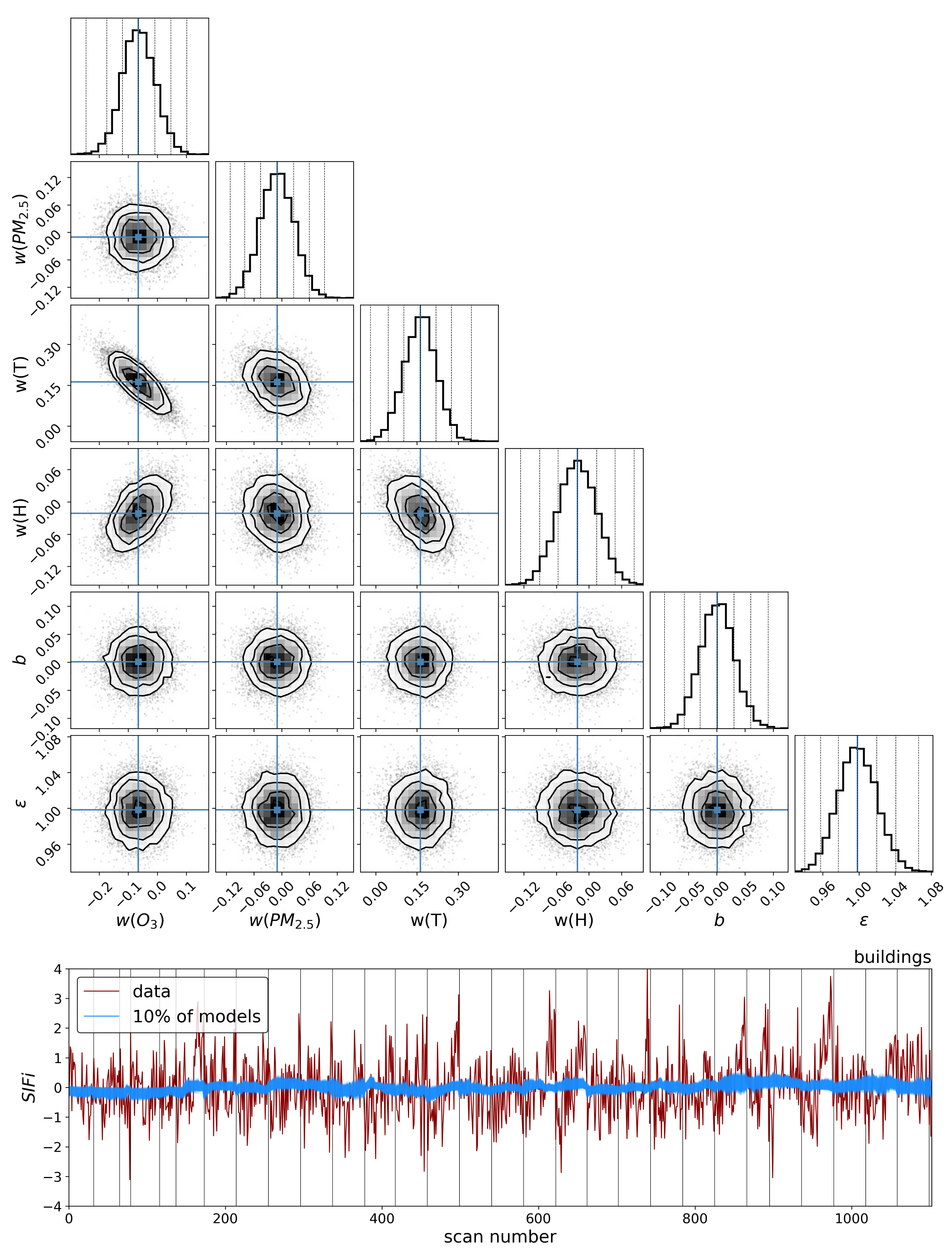
To explore the dependence of these vegetation health indicators on air quality, we model each indicator as a simple linear function of the air quality parameters:
where
is the quantified vegetation health measure extracted from the Compound Ratio spectra as a function of time and represents both the SIF indicator (
) as seen in
Section 3.1 and PCA component amplitudes in
Section 3.2,
is a vector containing the air quality parameter coefficients, and
contains the normalized measured O
3, PM
2.5, temperature (
T), and humidity (
H) as functions of time together with a constant. Markov Chain Monte Carlo (MCMC) sampling, implemented with the
emcee package in Python [
133], is used to estimate the probability distribution of the parameters
in each model. This MCMC approach generates samples of the likelihood function, which we define here as
where
y is the observed quantified vegetation health measure extracted from the spectra as a function of time and
represents an amount by which the noise is underestimated. By generating sufficient samples of the posterior surface, the maximum likelihood and (fully covariant) uncertainties for the air quality parameter coefficients
are determined.
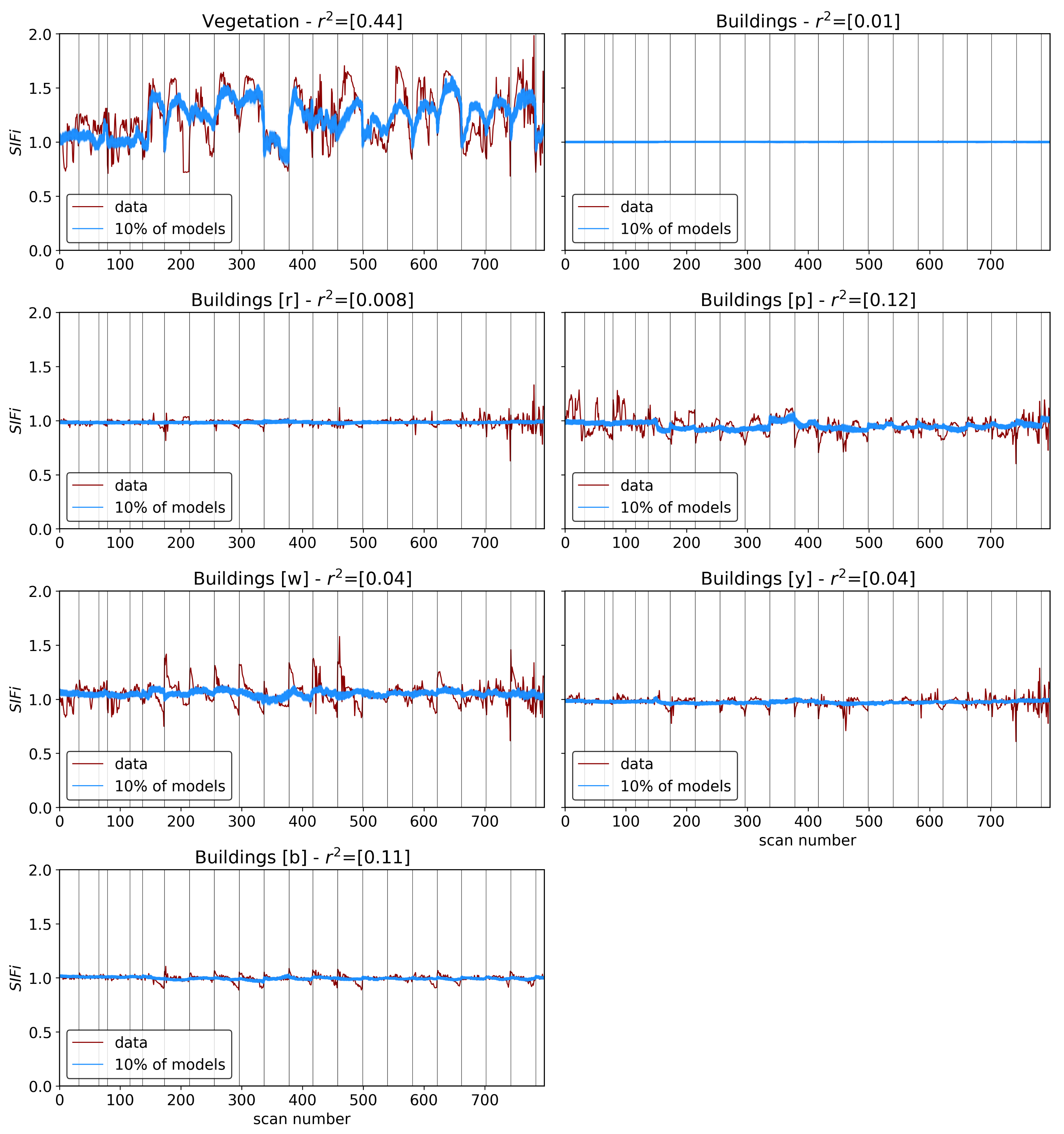
4. Discussion
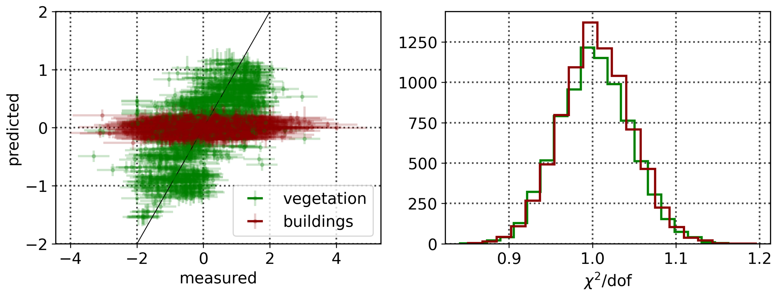
The results in the previous sections show that, regardless of the indicator used to quantify vegetation health, following our proposed method for atmospheric correction, there is a far stronger correlation between time-dependent changes in air quality and vegetation health than with that same indicator applied to nearby building spectra. Using the simple ratio of Compound Ratios at 0.75 μm to 0.9 μm to indicate the change in Solar-Induced Fluorescence (SIF), 40% of variation in the SIF indicator () with time is explained using the simple linear model of air quality parameters (O3, PM2.5, temperature, and humidity). On the other hand, <2% of the variation is explained in the values of buildings. Given that the changes provide cues concerning the health of vegetation, particularly the chlorophyll AB content and photosynthetic rates, it can be inferred from this result that the high explained variance of air quality parameters with changes is an indication that air quality is producing a measurable impact on the health of vegetation. Furthermore, all air quality parameter coefficients in the linear model of the for buildings are consistent with zero to within 3 uncertainty (fully covariant uncertainties derived from MCMC sampling of the likelihood), while none are consistent with zero for vegetation.
Similar results were obtained using Principal Component Analysis (PCA), where the variations in the amplitude of each of the four Principal Components (PCs) with time were used in the modeling. Component 1 showed an
of 38% for vegetation and 4% for buildings and, while components 2 and 3 showed lower correlation with changes in air quality than components 1 and 4, their correlations were still larger than those between building PCA amplitudes and air quality. Even though component 4 shows the least Explained Variance (EV) of 1.4%, it exhibited the strongest correlation of 47% for vegetation and only 4% for buildings. Interpreting this result is challenging since PCA produces components that are orthogonal by design and so explicating their structure as being representative of a physical property is not feasible. However, qualitatively assessing the shape of component 4 in
Figure 8 reveals characteristic structures such as an inverted green peak, red edge, and SIF peaks that are particularly effective at indicating vegetation health. The fact that the principal component with the least explained variance shows these features together with the greatest correlation with changes in air quality is an indication that much of the spectrum of vegetation does not contain important information regarding its health. At high spectral resolutions, it is inevitable that redundant information will be present, as well as temporal variation that is not related to vegetation health. Therefore, the practice of using the ratio of particular wavelengths, as is the case with the
, or dimensionality reduction processes such as PCA lends itself to extracting the essential information needed to infer vegetation health.
MCMC results showed a positive correlation for changes in ozone and temperature with changes in
values, and a negative correlation for variation in PM
2.5 and humidity. This result is also seen with NDVI in
Appendix A.1, and the opposite is seen in component 1 of PCA (noting that the amplitude of this component resembles the mean spectrum of vegetation reflected about the x-axis). Given the functional connection between photosynthesis and
, and the negative effects of PM
2.5 on photosynthetic rate, the obtained negative correlation is expected. Humidity is known to increase with increased opaque cloud cover [
139], which results in reduced sunshine and can therefore explain the resulting negative correlation with photosynthetic rate. Ozone, on the other hand, shows a counter-intuitive correlation given the known adverse effects it has on photosynthesis. The prevalent consensus in the literature over the past two decades suggests that increased surface ozone results in a decrease in chlorophyll content, causing adverse effects on tree biomass and visible leaf injury, leading to decreased photosynthesis [
21,
22,
23,
24]. However, studies demonstrating these effects are traditionally carried out under controlled environmental conditions using plant chambers to expose plants to known O
3 concentrations. While values vary by species, O
3 levels of 200–300 ppb are required for the impact on plant physiology to be measurable [
28]. Ozone levels in excess of 100 ppb are relatively rare in New York City, our data peak at ~80 ppb (see
Figure 5). Since O
3 does not accumulate in plant tissue and given the difficulty in separating its impacts from those of other environmental variables, conclusive proof of its impact on urban vegetation is lacking in the literature, and our results do not contradict previous findings. The positive correlation of ozone concentration with
values found in this work can potentially be explained by several environmental correlations and dependencies that cause this observed result. One such explanation is the co-occurrence of ozone with carbon dioxide. Since the Industrial Revolution, the concentrations of atmospheric carbon dioxide and ozone have increased in tandem [
140]. CO
2 generally enhances vegetation productivity and growth, and given the co-occurrence of O
3 and CO
2, the positive correlation obtained in this work between variations in vegetation health indicators and O
3 may be the result of increased CO
2 concentrations.
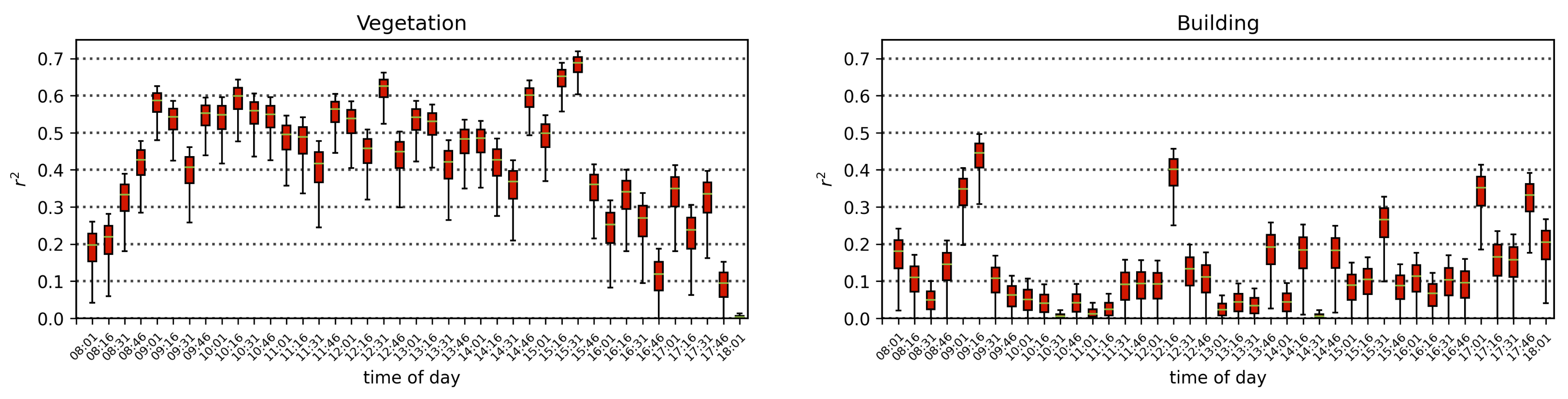
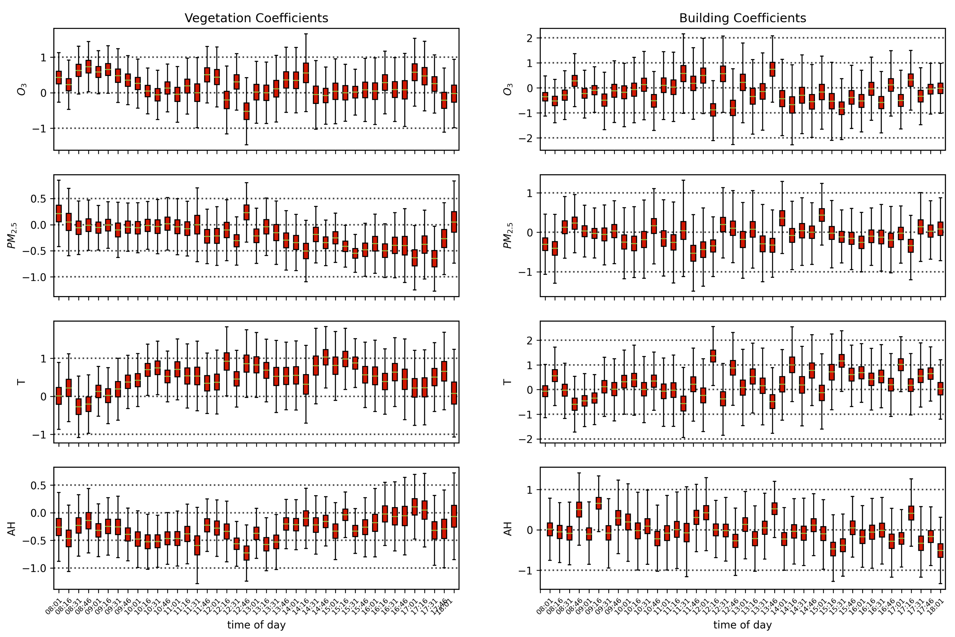
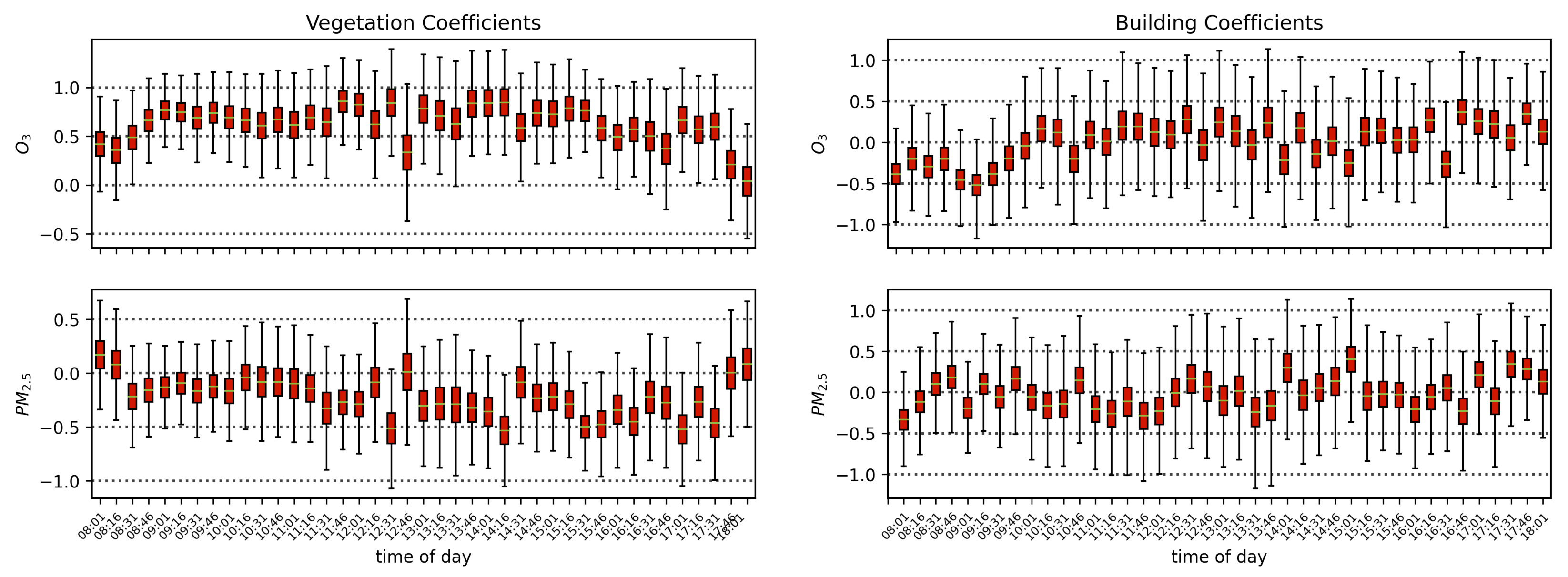
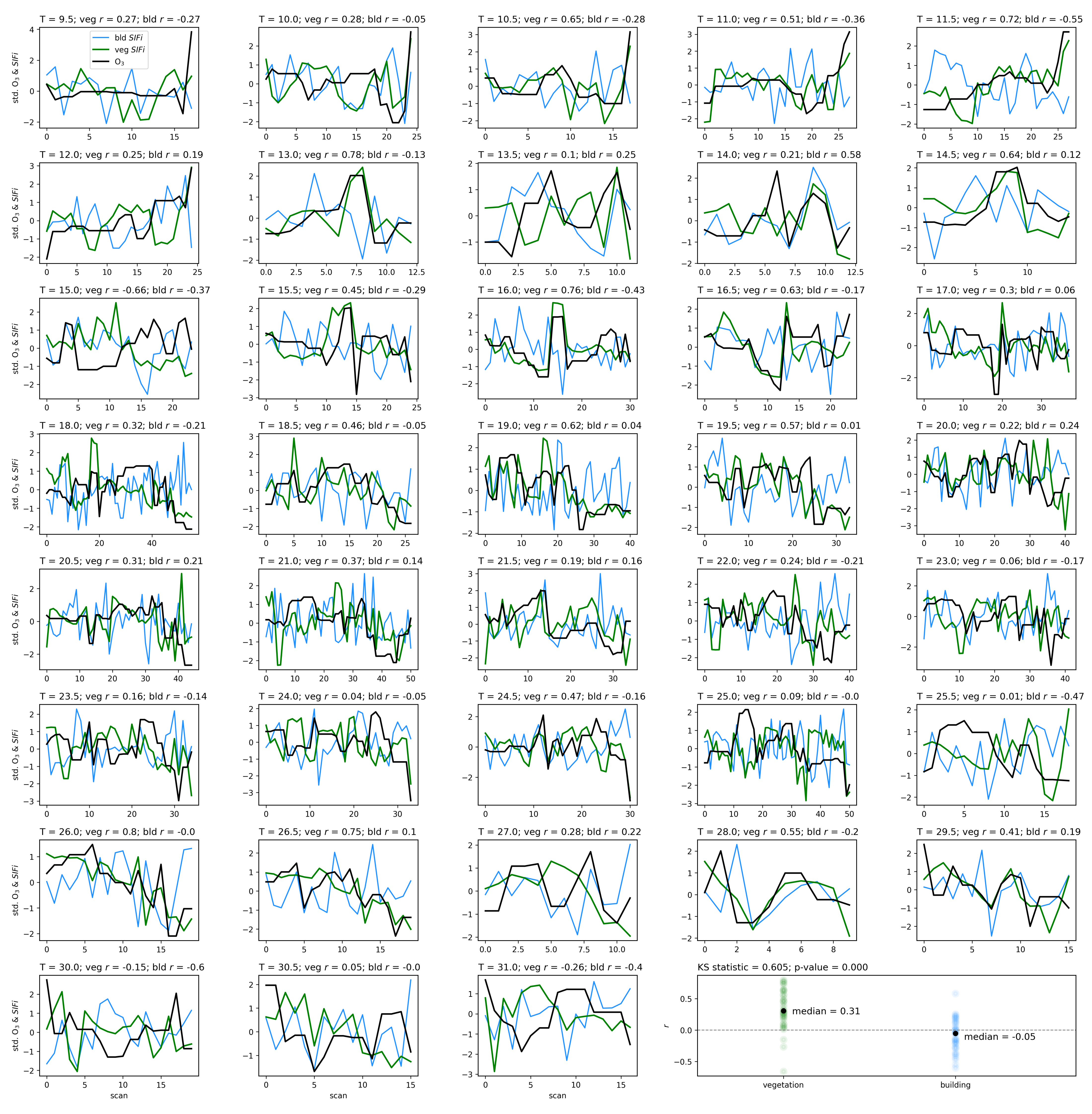
Air quality parameters, particularly O3 concentrations and temperatures, are known to exhibit a diurnal behavior that is correlated with solar angle. Solar-induced fluorescence is also known to vary with sun-sensor geometry, and with a fixed sensor view, the variation in solar zenith angle can result in a diurnal pattern in SIF that resembles the diurnal change in temperature, which also affects O3 concentrations. By separating the obtained scans into independent time series by the time of day of their acquisition, we isolate the impact of air quality from that of the diurnal cycle and observe that with a linear model of air quality parameters fit to each time-of-day series separately, the vegetation exhibits a median of 0.51, while the buildings show a far lower median value of 0.16. Furthermore, by isolating the scans into independent series based on their temperature, we find that vegetation on average has a Pearson’s correlation coefficient value of 0.31 with ozone, while the buildings’ is −0.05. These results show that while perhaps some correlation of air quality with vegetation health may be influenced by diurnal changes in solar angle and temperature, it is clear that the impact of O3 on vegetation health remains significant when controlling for solar angle and temperature.
In all test cases, the amount of variation explained by models fitting a linear combination of air quality parameters to the change in quantified measures of the spectra of vegetation was higher than that for buildings, however, it did not exceed 50%. The relatively low
in the vegetation models may be due to a variety of factors. While we expect that the effect is small given the unique spectrum of vegetation, one such factor is the accuracy of
k-means clustering, whereby non-vegetation pixels can potentially be mislabeled as vegetation. The inclusion of misidentified pixels could reduce the correlation with air quality if, for example, built structures are mislabeled as vegetation since (as we have found for building spectra) the correlation with air quality is weaker for built structures than vegetation. However, a likely more important consideration is that in this work we assume a simple linear combination of air quality parameters. Given the complexity in the interactions between air quality and vegetation, the results could potentially be improved using a more complex model. Finally, another important consideration potentially affecting the goodness of fit of the model is the fact that vegetation health is dependent on a complex variety and combination of factors besides the air quality parameters selected in this work. Vegetation health is also dependent on soil quality [
141], water runoff and retention [
142], direct sunlight and shade [
143], pests, disease, invasive species and weeds [
58,
61], and a plethora of other factors that are outside the scope of this work. Nonetheless, we argue that the
values for the linear air quality models and vegetation health found here are sufficient to indicate a robust correlation, especially in comparison with those obtained for the buildings.
5. Conclusions
Using a Visible and Near-Infrared (VNIR) single slit, scanning spectrograph, deployed by the Urban Observatory (UO) [
71,
72,
73,
74] in New York City, that captures 848 spectral channels in the 0.4–1.0 μm wavelength range, we obtained side-facing scans of an urban scene in 15 min intervals between 08h00 and 18h00 for 30 days between 3 May and 6 June 2016. Selecting vegetation pixels using unsupervised
k-means clustering, together with nearby building pixels split into two random sets (sets
a and
b) as controls, we present the use of the
Compound Ratio to remove the contribution of solar irradiance and atmospheric attenuation from the change in apparent reflectance in the mean spectra over time. We then correlated vegetation health indicators from the Compound Ratio of vegetation and buildings with publicly available concentrations of ozone (O
3) and particulate matter (PM
2.5), temperature, and humidity temporally coincident with the VNIR scans. For the vegetation health indicators, we used both a two-channel Solar-Induced Fluorescence (SIF) ratio of 0.75 μm to 0.9 μm (
) as well as amplitudes of a Principal Component Analysis (PCA) decomposition designed to capture broader spectral features.
Modeling these vegetation health indicators as a simple linear combination of the air quality and environmental parameters, and using Markov Chain Monte Carlo (MCMC) sampling of the likelihood to generate posterior distributions and determine parameter covariances, we found a strong correlation between changes in air quality parameters and variations in both indicators for vegetation health. Variations in values show significantly stronger correlation with air quality parameters for vegetation () compared to our control sample of buildings (), and all air quality parameter coefficients for the building model were consistent with zero to within 3 uncertainty. Similar results were obtained for PC amplitudes, with the strongest correlation between air quality parameters and variations in vegetation health measures found with the fourth PCA component (). By isolating the impact of the diurnal sun-sensor geometry on changes in solar-induced fluorescence, we show that the influence of air quality on vegetation health remains significant () in comparison with that of the buildings (). Furthermore, separating into series of constant temperature, we find that the impact of O3 on vegetation health is measurably independent of the correlations between diurnal sun-sensor geometry, solar-induced fluorescence, and temperature.
The strong correlation between a simple linear combination of air quality parameters and variations in all vegetation health indicators, especially the PCA decomposition results that encode information from the full resolution spectra, demonstrates the potential of reversing the analysis and using urban vegetation as a bioindicator for air quality. Specifically, the results indicate that it may be possible to extract the air quality parameters from the atmospherically corrected Compound Ratio spectra of urban vegetation by leveraging the ability of statistical models to learn coherent associations between the various spectral channels and their relation with air quality parameters. Evaluating the efficacy of such models to extract air quality from Compound Ratio spectra of vegetation as a function of spectral resolution will be the subject of future work.


