Article

Evaluation of Methods for Estimating Lake Surface Water Temperature Using Landsat 8

1
Laboratory of Applied Geoinformatics, Adam Mickiewicz University, Krygowskiego 10, 61-680 Poznan, Poland
2
Instituto Português do Mar e da Atmosfera (IPMA), 1749-077 Lisbon, Portugal
3
Department of Hydrology and Water Management, Adam Mickiewicz University, Krygowskiego 10, 61-680 Poznan, Poland
4
Department of Environmental Remote Sensing and Soil Science, Adam Mickiewicz University, Krygowskiego 10, 61-680 Poznan, Poland
5
Department of Land Improvement, Environmental Development and Spatial Management, Poznan University of Life Sciences, Piątkowska 94E, 60-649 Poznan, Poland
*
Author to whom correspondence should be addressed.
Remote Sens. 2022, 14(15), 3839; https://doi.org/10.3390/rs14153839
Submission received: 1 July 2022 / Revised: 29 July 2022 / Accepted: 4 August 2022 / Published: 8 August 2022
(This article belongs to the Special Issue Remote Sensing Image Processing in Poland)

Abstract

:
Changes in lake water temperature, observed with the greatest intensity during the last two decades, may significantly affect the functioning of these unique ecosystems. Currently, in situ studies in Poland are conducted only for 38 lakes using the single-point method. The aim of this study was to develop a method for remote sensing monitoring of lake water temperature in a spatio-temporal context based on Landsat 8 imagery. For this purpose, using data obtained for 28 lakes from the period 2013–2020, linear regression (LM) and random forest (RF) models were developed to estimate surface water temperature. In addition, analysis of Landsat Level-2 Surface Temperature Science Product (LST-L2) data provided by United States Geological Survey (USGS) and the National Aeronautics and Space Administration (NASA) was performed. The remaining 10 lakes not previously used in the model development stage were used to validate model performance. The results showed that the most accurate estimation is possible using the RF method for which RMSE = 1.83 °C and R2 = 0.89, while RMSE = 3.68 °C and R2 = 0.8 for the LST-L2 method. We found that LST-L2 contains a systematic error in the coastal zone, which can be corrected and eventually improve the quality of estimation. The satellite-based method makes it possible to determine water temperature for all lakes in Poland at different times and to understand the influence of climatic factors affecting temperature at the regional scale. On the other hand, spatial presentation of thermics within individual lakes enables understanding the influence of local factors and morphometric conditions.

Graphical Abstract

1. Introduction

Water ecosystems are characterized by considerable dynamics of energy and matter exchange, and therefore reflect modern transformations of the natural environment. Among the key properties of rivers and lakes is water temperature. Its course and distribution strongly determine a number of other processes [1]. It is therefore not surprising that the first water temperature measurements in lakes date back to the 18th century, and the frequency and accuracy of such measurements have been successively improving since. Traditional methods of temperature records based on in situ measurements are of point character, and are often not representative for complex and dynamic ecosystems such as lakes. The methods also have logistic limitations, and are costly and time consuming [2]. Moreover, the measurements are performed at various time intervals and at different depths, leading to high heterogeneity of the available data [3]. A complex understanding of the functioning of lake ecosystems requires collecting credible data on the state of water at the global scale, over long time periods, with high spatial and temporal resolution [2,4]. Data regarding the surface temperature of lakes have been collected using remote sensing for many years [5]. Satellite image data have been recorded at the global scale since 1972, when the first civil Earth observation mission commenced under the name Landsat (formerly known as the Earth Resources Technological Satellite). For the first time in the Landsat program, a sensor with a thermal band was installed on the Landsat 3 satellite (launched in 1978), but it quickly failed. Each of the following satellites of this program was equipped with sensors that recorded thermal radiation emitted from the Earth’s surface. An increase in water temperature in lakes shows a rate approximate to that of the growth of regional air temperature [6,7], although in the region of the Great Lakes and in northern Europe, a faster increase in lake water temperature was recorded than that of the surrounding air [7,8]. Satellite sensors used for the observation of the temperature of the surface water layer record emitted radiation at a range of 7–13 μm. The temperature of a very thin water layer is measured that can be referred to the temperature of the epilimnion in the conditions of lack of wind, although the external water layer is usually cooler than the 50 cm layer of sub-surface water [9]. Thermal scanners mounted on planes measure the temperature of the water layer on the interface of air and water with a thickness of 10–20 μm, but it can be several tenths of a degree warmer than temperature measured by a conventional sensor [10]. The difference between the temperature of the surface water layer and temperature in water depths is determined by factors such as the time of day, cloudiness, and wind speed [11,12]. To estimate the surface water temperature, data from one (“mono-window method”) or two (“split-window method”) thermal bands of the Landsat satellite can be used. The latter method is based on the difference in energy intensity in two thermal bands, which has the potential to improve temperature estimation [13]. In research determining the correlation between water temperature measured in situ and estimated from satellite data, thermal bands with low spatial resolution (i.e., Advanced Very High Resolution Radiometer) obtained very high values of determination coefficients (R2 > 0.9) [14]. Similar results were obtained using data from Landsat satellites with higher spatial resolution, although with lower temporal resolution. Tavares et al. [15] recommends the use of thermal data from the Landsat 7 ETM+ sensor for the observation of small lakes because at a relatively high spatial resolution the temperature estimation error is very close to the error obtained from the MODIS sensor (RMSE 1.07 and 1.05 °C, respectively). The usefulness of other medium-resolution thermal satellite sensors for water surface temperature assessment, such as Landsat TM, ETM+, TIRS [16,17,18,19,20] and Terra ASTER [21,22,23], was also investigated. Lake temperature is primarily determined by meteorological factors (insolation, cloudiness, air temperature, and wind speed), and to a lower degree by geomorphometric factors (surface area and depth) [24]. The temperature of the surface layer of the lake increases with its insolation, although an increase in temperature also causes cloudiness, because the amount of long-wave radiation reaching the surface increases [25]. A negative correlation occurs between water temperature and mean lake depth, i.e., shallow lakes warm up faster and to higher temperatures [26,27].
In the case of the territory of Poland, a lot of research has been recently conducted on lake water temperature, in reference to both measurement techniques [28,29] and improvement of methods of its modelling [30]. Polish lakes (approximately 7000 natural lakes in total) with multiannual in situ datasets are suitable for searching solutions in both of the aforementioned aspects of research. Water temperature measurements in Polish lakes have a history of several decades, and systematic observations commenced at the end of the 1950s. Over the years, the population of lakes covered by field measurements has changed, and today it concerns several tens of objects. No comprehensive research with the application of satellite images in reference to lake water temperature in Poland has been undertaken to date, although studies in the scope dynamically develop in different regions of the globe [31,32,33,34]. Polish research so far covers three lakes, and the obtained results revealed high cohesion with in situ measurements [35], encouraging a broader approach to the issue. Polish lakes already currently show a considerable increase in water temperature [29,36] that will continue to progress in the future [37,38].
The objective of this article is the comparison of four methods of estimation of water surface temperature in lakes in Poland based on thermal images from Landsat 8. Other detailed objectives include identification of limitations of the applied methods, and determination of the spatial variability of water temperature within the selected lakes and in a broader regional approach.

2. Materials and Methods

To organize the presentation of the results obtained in the subsequent stages, the following subsections were distinguished in this paper. Section 2.1 describes the study lakes, while Section 2.2 presents methods for conducting daily water temperature measurements. Section 2.3 and Section 2.4 describe the acquisition of Landsat 8 Collection 2 Level 1 (L8L1) data and Landsat Level-2 Surface Temperature Science Product data (LST-L2). Section 2.5, Section 2.6 and Section 2.7 describe the method of calculating lake water temperature using linear regression model (LM), random forest regression (RF), and Ermida et al. (2020) [39] method (LST), respectively. Section 2.8 describes the validation process. Finally, Section 2.9 shows the possibility of using results to present the spatial variability of water temperature at the scale of a single lake and at the regional scale for multiple lakes. The flowchart of this study is shown in Figure 1.

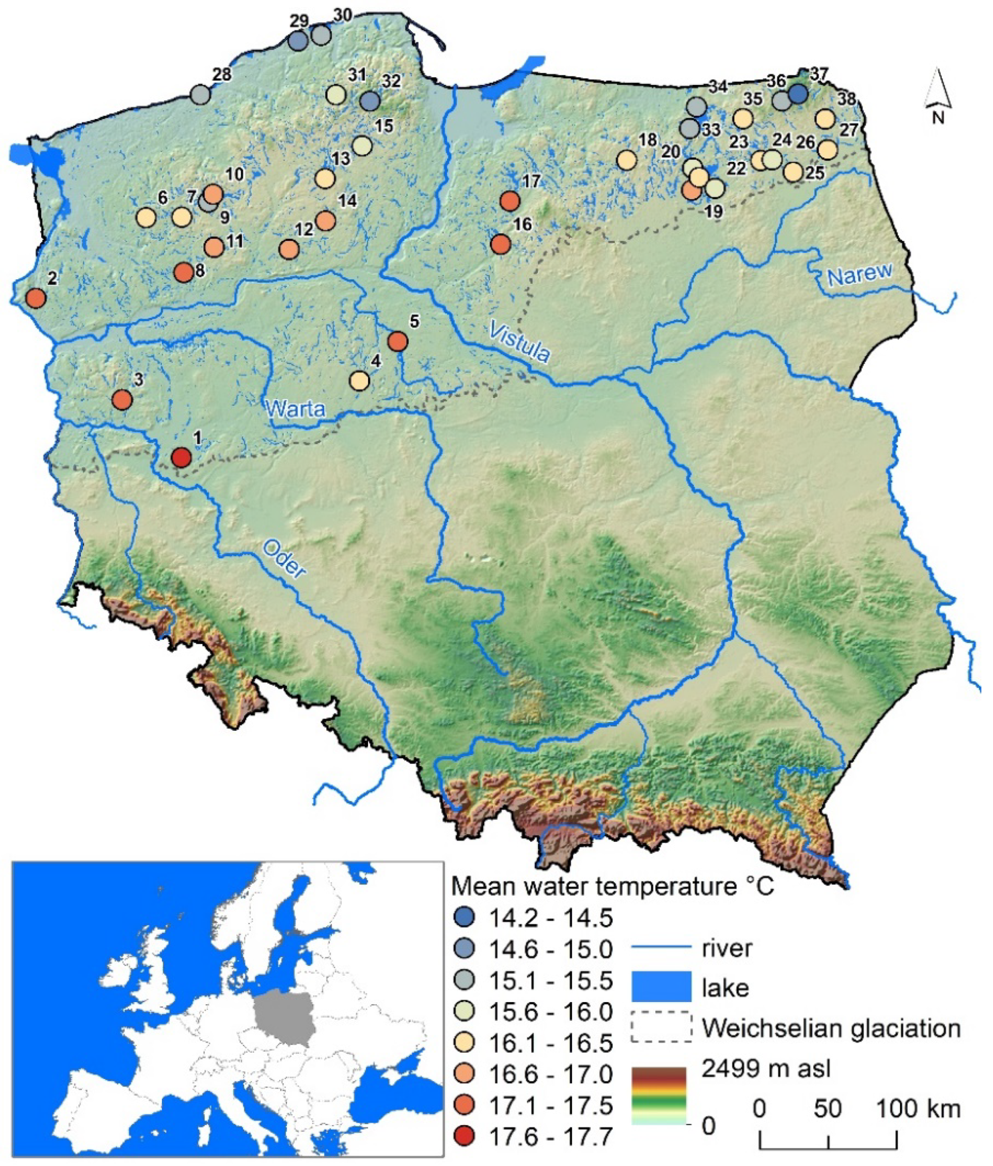
2.1. Study Sites Description

The analysis of the quality of water temperature determination based on satellite images from Landsat 8 covered 38 lakes in north Poland (Figure 2). All lakes selected for the analysis are natural water bodies. Their genesis is primarily related to the course of geomorphological processes during the Weichselian glaciation. The maximum extent of the ice during the Weichselian in north Poland is marked with a dotted line in Figure 2. It also constitutes the boundary of three main lakelands. The northern area of Poland is the richest in lakes, covering more than 500 lakes with a surface area larger than 1 km2. Lakes selected for the study have a variable surface area from 1.6 to 111.9 km2, and mean depths from 1.3 to 38.7 m. In genetic terms, postglacial lakes are largely dominant (channel, moraine, and kettle) related both to the erosional and accumulation activity of the Scandinavian ice sheet. Lakes developed in the Holocene also occur, namely Jamno (No. 28), Gardno (No. 29) and Łebsko (No. 30) which are also the northernmost study objects. Lake Sławskie (No. 1) is the southernmost one. Lake Morzycko (No. 2) is the westernmost lake, and Lake Studzieniczne (No. 27) has the easternmost location. Details of the morphometric parameters of lakes are presented in Supplementary Table S1. Mean annual temperatures of the analyzed lakes are at a level from 8.6 to 11.4 °C. In the regional approach, evident differences are observed in the period of winter–spring, when ice cover is still present on the lakes in the eastern part of Poland, but already absent in the lakes of west Poland. It is due to the features of transitional climate of the analyzed region, when a longer effect of cold continental air is recorded in the east.

2.2. In Situ Data

In this study, the results of daily water temperature measurements conducted between 2013 and 2020 by the Institute of Meteorology and Water Management—National Research Institute (IMWM) were used. The period from April to October, when there is generally no ice cover on the analyzed lakes, was selected for the analysis. Water temperature measurements by the IMWM are performed with a frequency of once a day at 6 UTC. The measurement points are located in the coastal zone and the sensor is placed approximately 0.4 m under the water level. Temperature measurements are performed both automatically and manually (especially for previous years), and their accuracy is 0.1 °C. Based on earlier hourly measurements of lake water temperature in Poland [40], it was evidenced that the difference between water temperature measurements at 6 UTC (in accordance with the IMWM standard) and ~9 UTC (overpass time of Landsat) in the summer half-year averages 0.1 °C, reflecting high thermal stability of water. Moreover, it should be emphasized that water temperature variability in the near-surface water layer (from the surface to a depth of 1 m) is inconsiderable, and as shown by earlier studies in the case of lakes in Poland [41], it averages 0.2 °C.

2.3. Landsat 8 TOA Data

In this paper, Landsat 8 data provided by the United States Geological Survey (USGS) was used. The data from April 2013 to October 2020 over north Poland were analyzed. The Landsat 8 Collection 2 Level 1 Tier 1 (L8L1) data were obtained using the Google Earth Engine (GEE; accessed on 24 February 2022) [42]. The L8L1 dataset contains calibrated top-of-atmosphere (TOA) reflectance derived from the data produced by the Operational Land Imager (OLI) and Thermal Infrared Sensor (TIRS). These L8L1 products contain 5 visible and near-infrared (VNIR) bands, 2 short-wave infrared (SWIR) bands with spatial resolution 30 m and 2 thermal infrared (TIR) bands resampled from 100 m to 30 m. Only scenes covering positions in the reference in situ data were considered (Figure 3). Due to the fact that in situ lake water temperature measurement sites are located within the shoreline range, it is not possible to obtain L8L1 data for these locations specifically. That results in the pixels (resolution 30 m) that extend over land or shoreline vegetation as well. Therefore, L8L1 data were collected from a point located 60 m inside the lake in relation to the in situ lake water temperature measurement sites. The water difference in this neighborhood is negligible, and we have the confidence to exclude pixels that are land. For the analysis all scenes with cloud cover less than 60% were taken. Moreover, we excluded data marked as clouds and cloud shadows based on the CFMask algorithm [43]. CFMask derives from the Function of Mask (FMask) developed by Zhu and Woodcock [44] and Zhu et al. [45]. Additionally, we removed data with reflectance values below 0, temperature values below 0 °C in thermal band B10, and outliers based on the ultra-blue band (B1 values ≥ 0.14). Additionally, some observations were made on two scenes on the same day—we treated them as duplicates and removed them.
Due to cloud cover patterns in Poland, for each of the analyzed lakes a slightly different imagery dataset was obtained. The least, 38 L8L1 images were acquired for Białe Augustowskie Lake (No. 26), while 83 images were acquired for Niesłysz Lake (No. 3). The dates for Niesłysz Lake (No. 3) are shown in Figure 4. The red dots indicate imageries that were rejected from the analysis and did not meet previously defined criteria, while the green dots indicate imageries that were used for estimating water temperature in the lake. Only 43% of all available scenes were suitable for analysis. Supplementary Figure S1 shows the exact availability of satellite scenes by lake, month, year and water temperature.

2.4. Landsat Level-2 Surface Temperature Science Product

In this paper, the results of Landsat Level-2 Surface Temperature Science Product provided by the USGS were used [46]. The LST-L2 product contains the temperature of the Earth’s surface in Kelvin (K). This product is generated mainly from the top-of-atmosphere thermal infrared data using a single-channel algorithm. Nevertheless, the algorithm is very extensive and uses auxiliary data, including data from the ASTER satellite and atmospheric data from reanalysis. The product is available in a resolution of 30 m as georeferenced rasters (.tif format) in the Universal Transverse Mercator coordinate system. Information on the applied techniques related to atmospheric compensation, calibration methodology, and validation are widely presented and discussed by Cook [47], Cook et al. [48], Malakar et al. [18], Schaeffer et al. [49]. In the case of LST-L2, the data availability differed for all analyzed lakes due to cloud cover pattern in Poland. From among all analyzed lakes, the least number of LST-L2 images, i.e., 38, was acquired for Biale Augustowskie Lake (No. 26), while the most number of 88 was acquired for Jamno Lake (No. 28).

2.5. Simple Linear Model

We used multiple linear regression as the first choice method because of its simplicity. The purpose of this model is to determine the relationship between multiple explanatory variables and the modelled (response) variable. In other words, we want to predict the unknown values of one variable based on the known values of other variables using the following formula:
f ( x ) = b 1 x 1 + b 2 x 2 + + b n x n + a
where
  • f ( x ) —is the response variable;
  • b 1 ,   b 2 ,   b n —are regression coefficients calculated for individual explanatory variables;
  • x 1 ,   x 2 ,   x n —are the values of the explanatory variables;
  • a —is the intercept.
Therefore, our modelled variable is water temperature and our explanatory variables are the two thermal bands B10 and B11. The main assumption of linear regression is the linear relationship between the modelled variable and the predictors, which is obviously not clear in the case of complex natural processes. However, this is not the only assumption—further limitations are related to the lack of multicollinearity, independence and normal distribution of errors, and a limited number of explanatory variables. For this reason, a more robust machine learning model may be a better solution.

2.6. Random Forest Model

Random Forest (RF) is a method that enables the estimation of searched values based on a large set of uncorrelated and random trees [50]. In our work, we used it for regression analysis. RF is based on bagging and random subspace methods. Bagging is related to the creation of regression trees, which are then combined into ensembles to obtain an overall prediction. To design regression trees, a number of independent bootstrap samples are created from the original training dataset. Each bootstrap sample (Db) is created by randomly sampling n subsamples from the original training data D, containing N subsamples. The bootstrap sample (Db) usually consists of 2/3 of D and contains no duplicate subsamples. Then, K independent regression trees are created for bootstrap samples with input vector x. In the regression analyses, the average prediction of the K regression trees, hk(x), is calculated to obtain an overall prediction [51,52] as follow,
y = 1 K k = 1 K   h k ( x )
Since the regression trees have high variance, the bagging is designed to reduce the variance and to prevent overfitting the complex RF model. Therefore, the learning trees cannot be correlated. Samples derived from the dataset that were not selected to train the k-th regression tree during the bagging process are compiled into an out-of-bag (OOB) subdataset. The OOB subdataset contains the remainder of D dataset (⅓ samples). Based on OOB subdataset, the performance of the k-th regression tree is calculated by the mean squared error (MSEOOB) as,
M S E O O B = 1 n i = 1 n ( y i y i ¯ ) 2
where y i and y i ¯ are the prediction and the mean of the i-th prediction from all regression trees. The determination coefficient R O O B 2 of the OOB subdataset, can be calculated based on MSEOOB and the total variance Vary, of the output parameter, using the following formula,
R O O B 2 = M S E O O B V a r y
The input data during the RF analyses were TOA reflectance values (B1, B2, B3, B4, B5, B6, B7, B10, and B11). Moreover, the spectral indices the Normalized Difference Vegetation Index (NDVI) [53] and the Normalized Difference Water Index (NDWI) [54], the month index as auxiliary variables to maximize prediction performance were used. All calculations related to the RF were accomplished using the ranger [55] package within the statistical software R 4.1.2 [56].

2.7. Land Surface Temperature Model

Ermida et al. (2020) [39] provides a code on GEE to derive LST from Landsat Collection 1 Level-1 thermal infrared bands. The method, referred to hereafter as LST, is based on the Statistical Mono-Window (SMW) algorithm developed by the Climate Monitoring Satellite Application Facility (CM-SAF) for deriving LST climate data records from Meteosat First and Second Generation [57]. The algorithm uses a single thermal infrared band (band 10 in the case of the Landsat 8) for consistency across all Landsat series. This method also uses the ASTER Global Emissivity Dataset (GED) database and applies vegetation cover correction based on Landsat NDVI. Since not all lakes considered in this study were correctly identified by the ASTER GED dataset, we have updated the code to use the Landsat water mask (available through the quality flag). For water bodies, the emissivity was set to 0.99.

2.8. Model Validation Procedure

To assess the accuracy of the LM, RF, LST and LST-L2 model predictions, we randomly selected 10 of the 38 lakes studied. In total, we used 538 in situ lake water temperature measurements to validate the temperature prediction results, which is approximately 23% of the input dataset. The root mean square error (RMSE), mean bias error (MBE), coefficient of Pearson correlation (R), between measured and predicted values were used for validation. Additionally, we calculated the standard deviation (SD) of the predicted values.

2.9. Model Application

Results obtained from the best model were used for the presentation of the spatial distribution of water temperature in lakes in the studied area at the local and regional scale. The objective of the presentation of the spatial variability of water temperature in single lakes was to show the role of local factors, i.e., the morphometry of the lake basin, range of impact of river waters, groundwater supply, and effect of wind on the distribution of water temperatures in the lake. The presentation of the thermal regime of lake waters at the regional scale aimed at illustrating the effect of climatic factors on the spatial distribution of water temperature in the lakes of north Poland in different time periods from April to October.
We tested the applicability of the developed RF model for the entire example scene of 28 April 2021 (ID: LC08_191023_20210428) and made the temperature prediction for 1568 lakes located in the north-western part of Poland with an area larger than 3 ha (approximately 30 pixels). On a local scale, we chose 4 lakes on different dates—Gopło, Łebsko, Drawsko, Ełckie (IDs: LC08_190023_20210608, LC08_191022_20150818, LC08_192023_20180529, and LC08_187022_20211025). We used the terra [58] package to process spatial data (both raster and vector) and perform spatial predictions.

3. Results

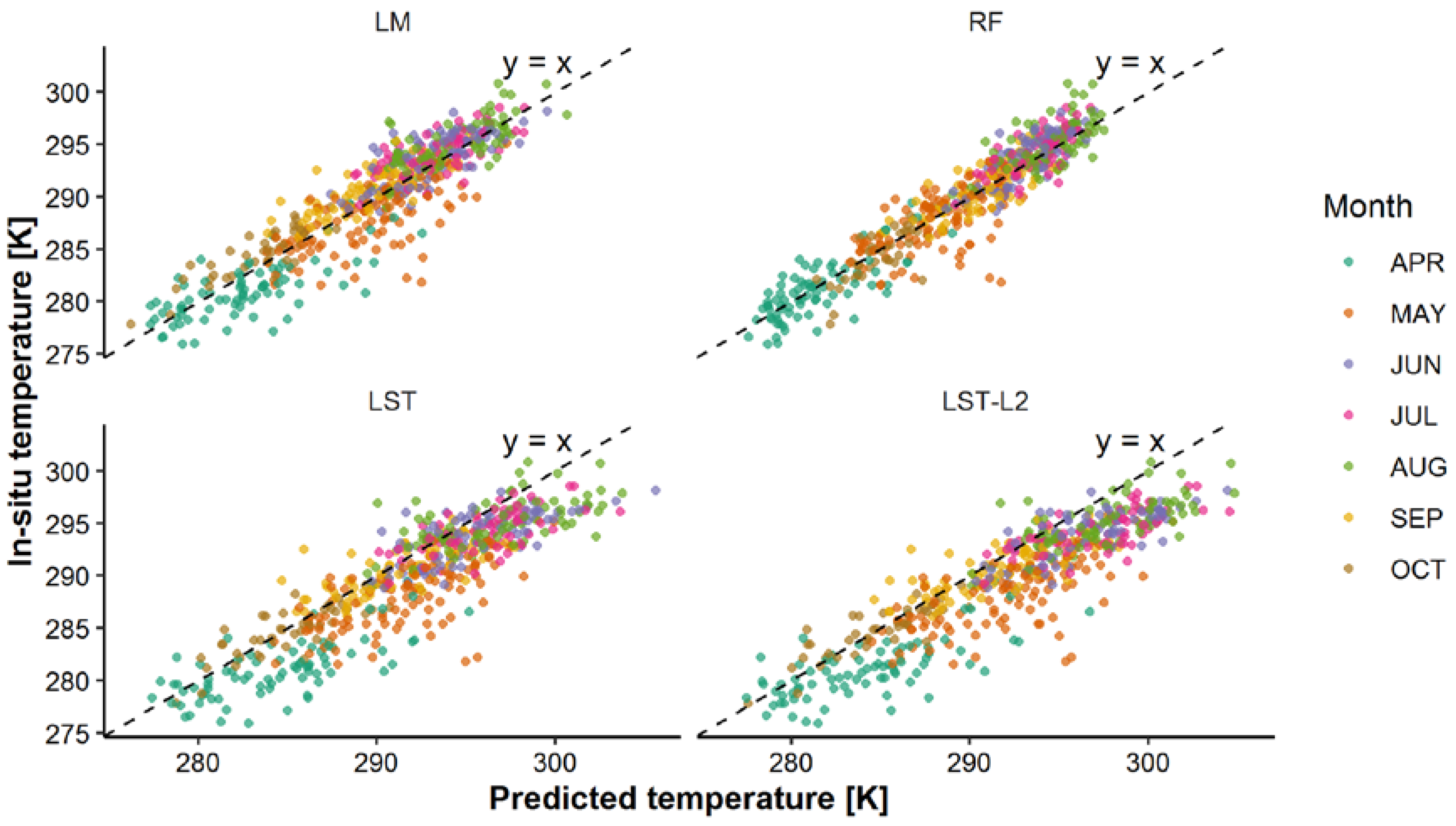
3.1. Comparison of Methods

At the first stage of work, based on a training sample covering measurement data from 28 lakes (1828 measurements) and the corresponding data from Landsat 8 Collection 2 Level 1 (L8L1) meeting the criteria described in the methodology, a multiple linear regression model (LM) was developed, as well as a random forest model (RF). The following equation parameters were obtained for the linear model:
Water temperature = 2.9 × B10 − 2.07 × B11 + 48.48
where bands B10 and B11 represent Top of Atmosphere Reflectance in Kelvins.
For model LM at the stage of development, the following statistics were obtained: R = 0.91, MBE = 0 °C, and RMSE = 2.28 °C. Considerably better statistics were obtained for the RF model, where the values were R = 0.95, MBE = 0.01 °C, and RMSE = 1.66 °C. Notice, however, that the RF algorithm strongly fits the training data. The analysis of the effectiveness of the RF model at the stage of its development within particular lakes showed very high results of correlation coefficients at a range from 0.98 to 1.0. MBE values were at a level from −0.52 to 0.58 °C, and RMSE values from 0.44 to 1.24 °C. The best results of temperature prediction at the stage of development of the RF model were obtained for Lake Ińsko (No. 6), and the worst for Lake Gopło (No. 5). Considering model LM, results obtained for particular lakes were as follows: R from 0.84 to 0.97, MBE from −1.48 to 1.86 °C, RMSE from 1.22 to 3.54 °C. The best results of temperature prediction at the stage of development of model LM were obtained for Lake Roś (No. 22), and the worst for Lake Gopło (No. 5). See Supplementary Table S2 for detailed results.
Considerably more credible from the point of view of further application of the model are results of the validation of statistical models on independent data not used at the stage of model development. The results are obviously worse than those obtained at the stage of model development. In this study, for LM, the obtained values R and RMSE were lower than in the case of RF model (Table 1). In the case of the LST model, RMSE values were almost twice higher than for results obtained from the RF model. The worst results of the estimation of lake water temperature were obtained for Landsat Level-2 Surface Temperature Science Product (LST-L2). In this case, MBE and RMSE values were 2.55 and 3.68 °C, respectively.
Considering the fact that next to values of global statistics obtained for the entire dataset, the selection of the appropriate model for the estimation of water temperature in lakes requires broader analysis, at least in the temporal approach—of particular months. In the period from April to October, a substantial change in water temperature occurs in particular lakes (from 0.3 °C to 28.3 °C), and a thermal gradient occurs from the east to the west of Poland modified between lakes by the impact of the Baltic Sea. The analysis of results obtained from the validation of LM and RF models evidently shows that RMSE results are lower than those obtained from finished products LST-L2 and LST (Table 2). An advantage of LST-L2 and LST models is their global cover and no requirement for measurement data for their calibration. The comparison of RMSE values between LM and RF models using the Wilcoxon signed-rank test showed a significant difference between them (p-value < 0.05). It suggested that RMSE values are lower for RF model than for LM. Differences between the estimation of water temperature are particularly evident in April (more than 1 °C), and the smallest differences occur in August (0.13 °C). Considering all models, the lowest RMSE values occur in October, and the highest in May. The analysis of the values of correlation coefficients for all methods showed that they are at a similar level, and the occurring differences are not statistically significant.
Results of the validation of the LM, RF, LST, and LST-L2 models are presented in Figure 5. The greatest dispersion of points presenting the comparison of measured and estimated values evidently occurs for April and May. According to Skowron [59], in that period water temperature shows high dynamics due to water mixing related to the development of stratification. Moreover, water temperatures estimated by means of the LST and LST-L2 models are evidently higher than the measured ones, suggesting the occurrence of a systematic error. For models RF and LM, the dispersion of points focuses within a straight line of y = x , suggesting the occurrence of only incidental/random errors.
Differences between measured water temperatures and those estimated by means of particular models are presented in Figure 6. Distributions of deviations obtained for the LST and LST-L2 models are evidently shifted right from the value of 0, pointing to the occurrence of systematic errors of 2.0 and 2.6 °C, respectively (for a testing sample of 10 lakes, 538 measurements). Due to this, improvement of the estimation of water temperatures can be relatively easily obtained by means of LST and LST-L2 by introducing a correction factor. Results of such analyses are presented in the next sub-chapter. In the case of the remaining LM and RF models, the average deviation between the measured and forecasted value is 0.0 and 0.1 °C, respectively. This points to the lack of occurrence of systematic errors. Histograms between actual and predicted values by all models indicate that they are normally distributed, although this is not apparent from the Shapiro–Wilk tests (p-value < 0.05). This is mainly due to single outliers.
The results obtained both globally and for individual months suggest that the best estimate of lake water temperature is possible using the RF model. This probably results, among others, from the fact that the collection of explanatory (independent) variables covers as many as 12 parameters (B1, B2, B3, B4, B5, B6, B7, B10, B11, the NDVI, the NDWI and the month index), and in LM only 2 parameters are used (B10 and B11). Therefore, an analysis of the suitability of the explanatory variables for estimating water temperature using the impurity algorithm from the random forest model was conducted (Figure 7). We found that B10 was more significant than B11, which is consistent with other publications. This is also confirmed by the result obtained for the linear model—a slightly higher Pearson correlation coefficient was noted for band B10 (R = 0.88) than for band B11 (R = 0.84). The results of the study by Barsi et al. [60] showed that due to the occurrence of out-of-field stray light, the calibration system of the TIR sensor is unstable, and the recorded thermal data may carry a substantial error. The effect of dispersed light on data recorded in band B10 is relatively small and therefore should be preferred. Considerably greater errors can occur in the case of data in band B11, they should be subject to additional external calibration. Another important variable is the month index—this is related to the seasonality of water temperature. Specifying the month significantly reduces errors resulting from incorrect satellite measurements. For example, in the warm months, we expect statistically higher temperatures than in the cold months. Thus, excluding weather anomalies, it can be expected that the water temperature range in June will be approximately from 18 °C (lower quartile) to 21.6 °C (upper quartile). The other variables are of little importance. Of the remaining spectral bands, the green band (B3) is the most significant. Green radiation that carries a lot of energy easily penetrates water. The depth of such penetration determines the magnitude of changes in water temperature, and depends on, among others, water transparency. Therefore, the amount of radiation reflected from water recorded in the green band can be related to water temperature [61,62,63].
We also evaluated the usefulness of spectral indices, the NDVI (used to calculate emissivity) and the NDWI (used to distinguish water from land), but they did not significantly affect the results.
Although the LM provides somewhat worse prediction results than the RF model, it has its evident advantages. Predictions of RF model employ 12 independent variables, which in the case of the analysis of the entire Landsat scene requires a total of approximately 5.4 GB RAM. In the case of LM, it will be only approximately 900 MB (2 variables). Next to the number of variables, the complexity of the model is also important—the linear model is much simpler, allowing for considerably faster prediction in terms of calculations. The last difference is related to the application of the month index—in the case of RF, it substantially improves prediction results, although it results in limiting the applicability of the model only to the geographic area of Poland (approximate latitudes and longitudes related to climate). In LM, no such assumptions were adopted; therefore, the potential of its applications is greater. Nonetheless, part of predictors can also be excluded post hoc in RF with no loss of effectiveness.
The spatial analysis of values of RMSE characteristics for the best RF model shows better adjustment of the model to the training sample of lakes (orange color) than for the test sample (points marked with red color) (Figure 8). The spatial analysis of RMSE values within the training sample showed no occurrence of spatial autocorrelation, i.e., grouping of lakes with evidently lower or higher RMSE values. Among the lakes used for testing the model, the lowest RMSE values were obtained for Lake Ełckie (No. 23): 1.40 °C. The highest RMSE values were obtained for Lake Hańcza (No. 37): 2.83 °C. Both Lakes Hańcza and Ełckie are located in east Poland. The correlation analysis between RMSE values and lakes’ areas, depths and volumes showed no significant relationship for both the training set and the test set.

3.2. LST-L2 Calibration

Because LST-L2 data are a finished product that can be practically applied by a large group of scientists, including hydrologists, limnologists, and water ecologists with no knowledge of specialized tools for obtaining and processing satellite data or development of statistical models (such as LM or RF), a decision was made to develop a calibration system for Poland for the estimation of water temperatures in lakes based on LST-L2 data provided by USGS. The analysis employed an identical method of determination of calibration parameters (based on 1828 measurements) and validation (538 measurements) as described in Section 2. The comparison of LST-L2 values with values of temperature measured in situ showed the occurrence of a systematic error of approximately 2.42 °C (Figure 9).
We tested three ways of correcting it using a linear equation (with and without an intercept) and adding the mean value of this error. We obtained successively RMSE values on the test set: 2.59, 2.86, and 2.88 °C (the initial RMSE value of LST-L2 was 3.68 °C). We strongly recommend calibrating the LST-L2 data for estimating the water surface temperature by using the formula below:
LST-L2 corrected = 0.806 × LST-L2 + 54.37

4. Discussion

Satellite images are an important tool in the case of research on water ecosystems, and find application in reference to many issues concerning both biotic [64,65,66] and abiotic processes [67,68,69]. A number of papers refer to the elementary feature, namely water temperature, and the applied methods analyze the issue at various temporal and spatial scales [15,70,71,72,73,74]. As mentioned in the introduction to this paper, research on lake water temperature in Poland with the application of satellite images has found no broader application to date, as confirmed by scarce papers in the scope. Ptak et al. [35] compared in situ water measurements with Landsat images (4, 5 and 7) for three coastal lakes, obtaining high coefficients of determination R2 (0.87–0.95). Based on in situ measurements and Landsat 8 data regarding surface water temperature in Lake Raduńskie Górne, Szkwarek and Wochna [75] obtained credible results allowing for detailed presentation of its spatial distribution. Monitoring programs are often based on a limited spatial and temporal range. Remote sensing offers promising tools for large-scale observation, improving our possibilities of comprehensive research of the indices of lake properties [32]. Therefore, in the context of dynamically progressing remote sensing technology, its limited scope of applicability in the analysis of lake water temperature in Poland constitutes a research gap that is attempted to be filled based on Landsat 8.
The application of Landsat images in this paper corresponds with the intensively addressed global research trend regarding lake water temperature. The applied methodical approach showed an RMSE error at a level of 1.8 °C, a result approximate to that in other studies using Landsat images. Simon et al. (2014), analyzing two freshwater lakes in France, determined the relationship between Landsat thermal data and water temperature by measuring the temperature in situ at various depths, from 0 to 0.5 m [20]. The authors concluded that the obtained results (R2 ranging from 0.90 to 0.94 and RMSE ranging from 1.753 to 2.397 °C) were satisfactory and coherent with literature data, where the values of mean square error are within a range from 1 to 2 °C. Giardino et al. [17] presented the Landsat TM-derived surface temperature of the sub-alpine lake with the RMSE of 0.328 °C; however, the procedure they used was not based on empirical relationships between satellite data and in situ measurements. For several hundred lakes analyzed based on data from the period 1999–2016 (Landsat 5 and 7), the total RMSE of temperature measurements obtained from the satellite was approximately 1.2 °C [19].
Mean absolute error for the analyzed lakes averaging from 1.38 to 2.39 °C (depending on the applied method) was approximate to the results of research conducted by Schaeffer et al. (2018) for lake waters in the United States, and reached 1.34 and 4.89 °C [49]. Results obtained in the study were also very approximate to those obtained by Tavares et al. (2019), who compared different methods of temperature estimation based on data from Landsat 7 and MODIS satellite [15]. In the estimation of water temperature (LSWT), the authors applied the single-channel algorithm method and two databases, SAFREE and TIGR3, obtaining similar R2 values (0.936 and 0.938, respectively) as in this study. A weaker correlation with in situ water temperature was also shown by MOD28 data from the MODIS satellite (R2 = 0.906), and a stronger one by MOD11 data (R2 = 0.962). The most useful for the estimation of temperature (R2 = 0.964) proved to be data from Landsat 7 satellite with the application of radiative transfer equation applied with atmospheric correction parameters from AtmCorr.
Considering the lack of possibility of conducting regular field observations, satellite remote sensing was recognized as a cost-effective way of monitoring water surface temperature at large spatial and temporal scales [76]. This statement is confirmed by results obtained in this paper, as exemplified by Figure 10, presenting a set of thermal data regarding three hundred lakes—including only several monitored through field observations. It should be emphasized that it is the first elaboration of the type for a fragment of the Polish territory, providing a promising basis for conducting monitoring of water temperature in lakes for a population of objects not achievable so far. Because water temperature is an elementary property of lake ecosystems [77,78] directly determining a number of processes and phenomena (biotic and abiotic), detailed information in the scope is necessary in reference to each lake. The obtained spatial image presented in Figure 10 points to the thermal variability of the analyzed lakes. The distribution in the orientation from the north (middle fragment) to the south is generally relatively clear, with occurrence of, respectively, cooler and warmer lakes. The situation illustrates the effect of a combination of environmental factors responsible for the thermal conditions of lakes. They include the surface area of the lake, land use structure around the lake, length, location (coordinates), and elevation above sea level [36]. According to the conducted research, multiple regression results showed that the recorded spatial distribution was significantly determined by, among others, the latitude, surface area, distance from the sea, presence of forests, and elevation above sea level. Similar research conducted for lakes on the Arctic coastal plain showed that, among others, parameters such as geographic location and morphometry of the lakes control their temperature at the regional scale [79].
The analyzed lakes with cooler water temperature occurred with greater density in the catchments of the Gwda and Drawa Rivers, on postglacial outwash plains built of highly permeable formations, i.e., gravels and sands. The situation is evident in the case of runoff, where the groundwater component is dominant in both of the aforementioned catchments [80], causing greater supply of cooler waters to the lakes.
Detailed distribution of water temperature is presented for two lakes with variable morphometric parameters (Figure 11). In both cases, certain patterns were recorded also observed in other studies of the type, i.e., distribution of water temperature referring to the depth of particular sectors of the lake and changes in water temperature in estuarial zones of rivers. According to Cao et al. [81], temperature in the center of the East Lake (Wuhan, China) is higher than in the surrounding area. Maps of surface temperature obtained by means of Landsat 8 satellite for three lakes (Maggiore, Lugano, and Como) showed variability reaching two or three degrees between different areas, i.e., between centers of lakes and coastal zones where inlets of rivers are located [82]. Based on data from Landsat 8 satellite, Sener and Sener [83] determined surface water temperature for Lake Beysehir (Turkey), recording a range of water temperature from 20.1 to 26.8 °C. They also determined that it was the highest in shallower sectors of the analyzed lake. Aïtelghazi et al. [84] emphasise that important parameters to be considered in the context of thermal changes include depth and suspended particles transported by the river. In the case of dimictic Lake Drawsko (Figure 11a), the distribution of water temperature in reference to depth is evident—the warmest in the coastal zone, and coldest in the deepest areas. A different situation is recorded in the case of polymictic Lake Łebsko (Figure 11b), where water temperature is uniform throughout the water column, and its variability on the surface is determined by inflows of surface waters—the coldest zone occurs in the south-eastern part (mouth of the Łeba River with average water flow), and in the north-eastern part (inflow of marine water), as well as in the north-western part, where a cooler water mass was pushed to an isolated bay with limited circulation.
The potential of Landsat images for monitoring small water bodies can be used for forecasting their evolution, and will be useful in the future [85]. It is important in the context of the progressing climate change and the related threat in reference to, among others, water quality or species composition of the fauna and flora of lake ecosystems.

5. Conclusions

This study concerned the comparison of the effectiveness of four methods of estimation of lake temperature based on satellite data. Two empirical models were developed (linear regression and random forest), and compared with two state of the art approaches employing atmospheric calibration. The comparative analysis shows the best performance of the random forest method, providing the highest correlation coefficient and the lowest RMSE.
Many papers recommend the application of atmospheric correction before using satellite data for the estimation of lake water temperature. It should be remembered, however, that the accuracy of these correction methods can be considerably reduced under certain conditions, e.g., with high content of water vapor in the atmosphere, and atmospheric models themselves show substantial limitations in spatial and temporal resolution. Therefore, continuous work on the improvement of correction algorithms should be accompanied by research on the possibility of application of new methods of data analysis (e.g., machine learning) and consideration of empirical data in the improvement of prediction results. This paper proposes an appropriate calibration correction for data from Landsat Level-2 Surface Temperature Science Product (LST-L2) that considerably improves results (root mean square error reduced by 30%) of estimation of lake temperature in the territory of Poland. Nevertheless, despite the correction, the random forest model provided the best results.
Future works should focus on determining the pixel based temperature uncertainty, analyzing the potential of using low-resolution data from the MODIS sensor for small surface lakes in Poland and determining the effectiveness of other water and vegetation indices. As of 31 October 2021, imagery is available from the next Landsat series satellite with the improved TIRS-2 sensor. Along with the increase in data availability, it should also be used for analysis to maintain continuous monitoring.

Supplementary Materials

The following supporting information can be downloaded at: https://www.mdpi.com/article/10.3390/rs14153839/s1, Table S1: Morphometric parameters of the analyzed lakes. Table S2: Linear and random forest model performance per lake on train and test sets. Test lakes are marked with “x”. Figure S1: Availability of satellite scenes depending on (a) lake; (b) month; (c) year; (d) water temperature (as intervals). Reference [86] is cited in the Supplementary Table S1.

Author Contributions

K.D.: methodology, software, validation, formal analysis, data curation, writing—original draft preparation, review, editing, and visualization. S.E.: software and writing—review, editing. M.P.: writing—original draft preparation, review, and editing. J.P.: writing—original draft preparation, review, and editing. M.S.: formal analysis, writing—original draft preparation, review, editing, and visualization. All authors have read and agreed to the published version of the manuscript.

Funding

This research received no external funding.

Data Availability Statement

In this study, we used publicly available datasets. Hydrologic data, satellite measurements, random forest regression model, and statistical analysis results are available in this repository: https://github.com/kadyb/lakes_temp (accessed on 1 May 2022). This repository also includes fully functional and reproducible codes under the MIT license.

Acknowledgments

The source of the hydrological data is the Institute of Meteorology and Water Management—National Research Institute (https://www.imgw.pl/). Landsat-8 images courtesy of the U.S. Geological Survey (https://earthexplorer.usgs.gov/). Both websites accessed on 1 May 2022.

Conflicts of Interest

The authors declare no conflict of interest.

References

  1. Ptak, M.; Sojka, M.; Graf, R.; Choiński, A.; Zhu, S.; Nowak, B. Warming Vistula River—The Effects of Climate and Local Conditions on Water Temperature in One of the Largest Rivers in Europe. J. Hydrol. Hydromech. 2022, 70, 1–11. [Google Scholar] [CrossRef]
  2. Hestir, E.L.; Brando, V.E.; Bresciani, M.; Giardino, C.; Matta, E.; Villa, P.; Dekker, A.G. Measuring Freshwater Aquatic Ecosystems: The Need for a Hyperspectral Global Mapping Satellite Mission. Remote Sens. Environ. 2015, 167, 181–195. [Google Scholar] [CrossRef] [Green Version]
  3. Lieberherr, G.; Wunderle, S. Lake Surface Water Temperature Derived from 35 Years of AVHRR Sensor Data for European Lakes. Remote Sens. 2018, 10, 990. [Google Scholar] [CrossRef] [Green Version]
  4. van Puijenbroek, P.J.T.M.; Evers, C.H.M.; van Gaalen, F.W. Evaluation of Water Framework Directive Metrics to Analyse Trends in Water Quality in the Netherlands. Sustain. Water Qual. Ecol. 2015, 6, 40–47. [Google Scholar] [CrossRef]
  5. Birk, S.; Ecke, F. The Potential of Remote Sensing in Ecological Status Assessment of Coloured Lakes Using Aquatic Plants. Ecol. Indic. 2014, 46, 398–406. [Google Scholar] [CrossRef]
  6. Livingstone, D.M.; Lotter, A.F. The Relationship between Air and Water Temperatures in Lakes of the Swiss Plateau: A Case Study with Palaeolimnological Implications. J. Paleolimnol. 1998, 19, 181–198. [Google Scholar] [CrossRef]
  7. Schneider, P.; Hook, S.J. Space Observations of Inland Water Bodies Show Rapid Surface Warming since 1985. Geophys. Res. Lett. 2010, 37, L22405. [Google Scholar] [CrossRef] [Green Version]
  8. Austin, J.; Colman, S. A Century of Temperature Variability in Lake Superior. Limnol. Oceanogr. 2008, 53, 2724–2730. [Google Scholar] [CrossRef]
  9. Crosman, E.T.; Horel, J.D. MODIS-Derived Surface Temperature of the Great Salt Lake. Remote Sens. Environ. 2009, 113, 73–81. [Google Scholar] [CrossRef]
  10. George, G.D. Using Airborne Remote Sensing to Study the Physical Dynamics of Lakes and the Spatial Distribution of Phytoplankton. Freshw. Rev. 2012, 5, 121–140. [Google Scholar] [CrossRef]
  11. Schluessel, P.; Emery, W.J.; Grassl, H.; Mammen, T. On the Bulk-Skin Temperature Difference and Its Impact on Satellite Remote Sensing of Sea Surface Temperature. J. Geophys. Res. 1990, 95, 13341. [Google Scholar] [CrossRef]
  12. Wick, G.A.; Emery, W.J.; Kantha, L.H.; Schlüssel, P. The Behavior of the Bulk—Skin Sea Surface Temperature Difference under Varying Wind Speed and Heat Flux. J. Phys. Oceanogr. 1996, 26, 1969–1988. [Google Scholar] [CrossRef]
  13. Rozenstein, O.; Qin, Z.; Derimian, Y.; Karnieli, A. Derivation of Land Surface Temperature for Landsat-8 TIRS Using a Split Window Algorithm. Sensors 2014, 14, 5768–5780. [Google Scholar] [CrossRef]
  14. Politi, E.; Cutler, M.E.J.; Rowan, J.S. Using the NOAA Advanced Very High Resolution Radiometer to Characterise Temporal and Spatial Trends in Water Temperature of Large European Lakes. Remote Sens. Environ. 2012, 126, 1–11. [Google Scholar] [CrossRef] [Green Version]
  15. Tavares, M.; Cunha, A.; Motta-Marques, D.; Ruhoff, A.; Cavalcanti, J.; Fragoso, C.; Martín Bravo, J.; Munar, A.; Fan, F.; Rodrigues, L. Comparison of Methods to Estimate Lake-Surface-Water Temperature Using Landsat 7 ETM+ and MODIS Imagery: Case Study of a Large Shallow Subtropical Lake in Southern Brazil. Water 2019, 11, 168. [Google Scholar] [CrossRef] [Green Version]
  16. Cheval, S.; Popa, A.-M.; Șandric, I.; Iojă, I.-C. Exploratory Analysis of Cooling Effect of Urban Lakes on Land Surface Temperature in Bucharest (Romania) Using Landsat Imagery. Urban Clim. 2020, 34, 100696. [Google Scholar] [CrossRef]
  17. Giardino, C.; Pepe, M.; Brivio, P.A.; Ghezzi, P.; Zilioli, E. Detecting Chlorophyll, Secchi Disk Depth and Surface Temperature in a Sub-Alpine Lake Using Landsat Imagery. Sci. Total Environ. 2001, 268, 19–29. [Google Scholar] [CrossRef]
  18. Malakar, N.K.; Hulley, G.C.; Hook, S.J.; Laraby, K.; Cook, M.; Schott, J.R. An Operational Land Surface Temperature Product for Landsat Thermal Data: Methodology and Validation. IEEE Trans. Geosci. Remote Sens. 2018, 56, 5717–5735. [Google Scholar] [CrossRef]
  19. Prats, J.; Reynaud, N.; Rebière, D.; Peroux, T.; Tormos, T.; Danis, P.-A. LakeSST: Lake Skin Surface Temperature in French Inland Water Bodies for 1999–2016 from Landsat Archives. Earth Syst. Sci. Data 2018, 10, 727–743. [Google Scholar] [CrossRef] [Green Version]
  20. Simon, R.N.; Tormos, T.; Danis, P.-A. Retrieving Water Surface Temperature from Archive LANDSAT Thermal Infrared Data: Application of the Mono-Channel Atmospheric Correction Algorithm over Two Freshwater Reservoirs. Int. J. Appl. Earth Obs. Geoinf. 2014, 30, 247–250. [Google Scholar] [CrossRef]
  21. Becker, M.; Daw, A. Influence of Lake Morphology and Clarity on Water Surface Temperature as Measured by EOS ASTER. Remote Sens. Environ. 2005, 99, 288–294. [Google Scholar] [CrossRef]
  22. Kay, J.E.; Kampf, S.K.; Handcock, R.N.; Cherkauer, K.A.; Gillespie, A.R.; Burges, S.J. Accuracy of Lake and Stream Temperatures Estimated from Thermal Infrared Images. J. Am. Water Resour. Assoc. 2005, 41, 1161–1175. [Google Scholar] [CrossRef]
  23. Sabol, D.E., Jr.; Gillespie, A.R.; Abbott, E.; Yamada, G. Field Validation of the ASTER Temperature–Emissivity Separation Algorithm. Remote Sens. Environ. 2009, 113, 2328–2344. [Google Scholar] [CrossRef]
  24. Sharma, S.; Walker, S.C.; Jackson, D.A. Empirical Modelling of Lake Water-Temperature Relationships: A Comparison of Approaches. Freshw. Biol. 2008, 53, 897–911. [Google Scholar] [CrossRef]
  25. Edinger, J.E.; Duttweiler, D.W.; Geyer, J.C. The Response of Water Temperatures to Meteorological Conditions. Water Resour. Res. 1968, 4, 1137–1143. [Google Scholar] [CrossRef]
  26. Oswald, C.J.; Rouse, W.R. Thermal Characteristics and Energy Balance of Various-Size Canadian Shield Lakes in the Mackenzie River Basin. J. Hydrometeorol. 2004, 5, 129–144. [Google Scholar] [CrossRef]
  27. Snucins, E.; John, G. Interannual Variation in the Thermal Structure of Clear and Colored Lakes. Limnol. Oceanogr. 2000, 45, 1639–1646. [Google Scholar] [CrossRef]
  28. Choiński, A.; Ptak, M.; Strzelczak, A. Changeability of Accumulated Heat Content in Alpine-Type Lakes. Pol. J. Environ. Stud. 2015, 24, 2363–2369. [Google Scholar] [CrossRef]
  29. Ptak, M.; Sojka, M.; Kozłowski, M. The Increasing of Maximum Lake Water Temperature in Lowland Lakes of Central Europe: Case Study of the Polish Lakeland. Ann. Limnol. Int. J. Limnol. 2019, 55, 6. [Google Scholar] [CrossRef]
  30. Heddam, S.; Ptak, M.; Zhu, S. Modelling of Daily Lake Surface Water Temperature from Air Temperature: Extremely Randomized Trees (ERT) versus Air2Water, MARS, M5Tree, RF and MLPNN. J. Hydrol. 2020, 588, 125130. [Google Scholar] [CrossRef]
  31. De Santis, D.; Del Frate, F.; Schiavon, G. Analysis of Climate Change Effects on Surface Temperature in Central-Italy Lakes Using Satellite Data Time-Series. Remote Sens. 2021, 14, 117. [Google Scholar] [CrossRef]
  32. Huovinen, P.; Ramírez, J.; Caputo, L.; Gómez, I. Mapping of Spatial and Temporal Variation of Water Characteristics through Satellite Remote Sensing in Lake Panguipulli, Chile. Sci. Total Environ. 2019, 679, 196–208. [Google Scholar] [CrossRef]
  33. Irani Rahaghi, A.; Lemmin, U.; Barry, D.A. Surface Water Temperature Heterogeneity at Subpixel Satellite Scales and Its Effect on the Surface Cooling Estimates of a Large Lake: Airborne Remote Sensing Results From Lake Geneva. J. Geophys. Res. Ocean. 2019, 124, 635–651. [Google Scholar] [CrossRef] [Green Version]
  34. Yu, Z.; Yang, K.; Luo, Y.; Wang, P.; Yang, Z. Research on the Lake Surface Water Temperature Downscaling Based on Deep Learning. IEEE J. Sel. Top. Appl. Earth Obs. Remote Sens. 2021, 14, 5550–5558. [Google Scholar] [CrossRef]
  35. Ptak, M.; Choiński, A.; Piekarczyk, J.; Pryłowski, T. Applying Landsat Satellite Thermal Images in the Analysis of Polish Lake Temperatures. Pol. J. Environ. Stud. 2017, 26, 2159–2165. [Google Scholar] [CrossRef]
  36. Ptak, M.; Sojka, M.; Choiński, A.; Nowak, B. Effect of Environmental Conditions and Morphometric Parameters on Surface Water Temperature in Polish Lakes. Water 2018, 10, 580. [Google Scholar] [CrossRef] [Green Version]
  37. Czernecki, B.; Ptak, M. The Impact of Global Warming on Lake Surface Water Temperature in Poland—The Application of Empirical-Statistical Downscaling, 1971–2100. J. Limnol. 2018, 77, 330–348. [Google Scholar] [CrossRef]
  38. Piccolroaz, S.; Zhu, S.; Ptak, M.; Sojka, M.; Du, X. Warming of Lowland Polish Lakes under Future Climate Change Scenarios and Consequences for Ice Cover and Mixing Dynamics. J. Hydrol. Reg. Stud. 2021, 34, 100780. [Google Scholar] [CrossRef]
  39. Ermida, S.L.; Soares, P.; Mantas, V.; Göttsche, F.-M.; Trigo, I.F. Google Earth Engine Open-Source Code for Land Surface Temperature Estimation from the Landsat Series. Remote Sens. 2020, 12, 1471. [Google Scholar] [CrossRef]
  40. Ptak, M.; Sojka, M.; Nowak, B. Characteristics of Daily Water Temperature Fluctuations in Lake Kierskie (West Poland). Quaest. Geogr. 2019, 38, 41–49. [Google Scholar] [CrossRef] [Green Version]
  41. Ptak, M.; Nowak, B. Variability of Oxygen-Thermal Conditions in Selected Lakes in Poland. Ecol. Chem. Eng. 2016, 23, 639–650. [Google Scholar] [CrossRef] [Green Version]
  42. Gorelick, N.; Hancher, M.; Dixon, M.; Ilyushchenko, S.; Thau, D.; Moore, R. Google Earth Engine: Planetary-Scale Geospatial Analysis for Everyone. Remote Sens. Environ. 2017, 202, 18–27. [Google Scholar] [CrossRef]
  43. Foga, S.; Scaramuzza, P.L.; Guo, S.; Zhu, Z.; Dilley, R.D.; Beckmann, T.; Schmidt, G.L.; Dwyer, J.L.; Joseph Hughes, M.; Laue, B. Cloud Detection Algorithm Comparison and Validation for Operational Landsat Data Products. Remote Sens. Environ. 2017, 194, 379–390. [Google Scholar] [CrossRef] [Green Version]
  44. Zhu, Z.; Woodcock, C.E. Object-Based Cloud and Cloud Shadow Detection in Landsat Imagery. Remote Sens. Environ. 2012, 118, 83–94. [Google Scholar] [CrossRef]
  45. Zhu, Z.; Wang, S.; Woodcock, C.E. Improvement and Expansion of the Fmask Algorithm: Cloud, Cloud Shadow, and Snow Detection for Landsats 4–7, 8, and Sentinel 2 Images. Remote Sens. Environ. 2015, 159, 269–277. [Google Scholar] [CrossRef]
  46. USGS Landsat 8-9 Collection 2 (C2) Level 2 Science Product (L2SP) Guide; United States Geological Survey: Asheville, NC, USA, 2022; pp. 1–42.
  47. Cook, M. Atmospheric Compensation for a Landsat Land Surface Temperature Product; Rochester Institute of Technology: Rochester, NY, USA, 2014. [Google Scholar]
  48. Cook, M.; Schott, J.; Mandel, J.; Raqueno, N. Development of an Operational Calibration Methodology for the Landsat Thermal Data Archive and Initial Testing of the Atmospheric Compensation Component of a Land Surface Temperature (LST) Product from the Archive. Remote Sens. 2014, 6, 11244–11266. [Google Scholar] [CrossRef] [Green Version]
  49. Schaeffer, B.A.; Iiames, J.; Dwyer, J.; Urquhart, E.; Salls, W.; Rover, J.; Seegers, B. An Initial Validation of Landsat 5 and 7 Derived Surface Water Temperature for U.S. Lakes, Reservoirs, and Estuaries. Int. J. Remote Sens. 2018, 39, 7789–7805. [Google Scholar] [CrossRef]
  50. Breiman, L. Random Forests. Mach. Learn. 2001, 45, 5–32. [Google Scholar] [CrossRef] [Green Version]
  51. Ganesh, N.; Jain, P.; Choudhury, A.; Dutta, P.; Kalita, K.; Barsocchi, P. Random Forest Regression-Based Machine Learning Model for Accurate Estimation of Fluid Flow in Curved Pipes. Processes 2021, 9, 2095. [Google Scholar] [CrossRef]
  52. Seo, D.; Kim, Y.; Eo, Y.; Park, W.; Park, H. Generation of Radiometric, Phenological Normalized Image Based on Random Forest Regression for Change Detection. Remote Sens. 2017, 9, 1163. [Google Scholar] [CrossRef] [Green Version]
  53. Rouse, J.W., Jr.; Haas, R.H.; Deering, D.W.; Schell, J.A.; Harlan, J.C. Monitoring the Vernal Advancement and Retrogradation (Green Wave Effect) of Natural Vegetation; Texas A&M University: College Station, TX, USA, 1974. [Google Scholar]
  54. McFeeters, S.K. The Use of the Normalized Difference Water Index (NDWI) in the Delineation of Open Water Features. Int. J. Remote Sens. 1996, 17, 1425–1432. [Google Scholar] [CrossRef]
  55. Wright, M.N.; Ziegler, A. Ranger: A Fast Implementation of Random Forests for High Dimensional Data in C++ and R. J. Stat. Softw. 2017, 77, 1–17. [Google Scholar] [CrossRef] [Green Version]
  56. R Core Team. R: A Language and Environment for Statistical Computing; R Core Team: Vienna, Austria, 2022. [Google Scholar]
  57. Duguay-Tetzlaff, A.; Bento, V.; Göttsche, F.; Stöckli, R.; Martins, J.; Trigo, I.; Olesen, F.; Bojanowski, J.; da Camara, C.; Kunz, H. Meteosat Land Surface Temperature Climate Data Record: Achievable Accuracy and Potential Uncertainties. Remote Sens. 2015, 7, 13139–13156. [Google Scholar] [CrossRef] [Green Version]
  58. Hijmans, R.J. Terra: Spatial Data Analysis, USA, 2022.
  59. Skowron, R. Zróżnicowanie i Zmienność Wybranych Elementów Reżimu Termicznego Wody w Jeziorach Na Niżu Polskim; Uniwersytetu Mikołaja Kopernika: Toruń, Poland, 2011; ISBN 978-83-231-2695-9. [Google Scholar]
  60. Barsi, J.; Schott, J.; Hook, S.; Raqueno, N.; Markham, B.; Radocinski, R. Landsat-8 Thermal Infrared Sensor (TIRS) Vicarious Radiometric Calibration. Remote Sens. 2014, 6, 11607–11626. [Google Scholar] [CrossRef] [Green Version]
  61. Hashim, N.S.; Windupranata, W.; Sulaiman, S.A.H. Shallow-Water Bathymetry Estimation Using Single Band Algorithm and Green Band Algorithm. In Proceedings of the 2020 11th IEEE Control and System Graduate Research Colloquium (ICSGRC), Shah Alam, Malaysia, 8 August 2020; pp. 214–219. [Google Scholar]
  62. Jia, X.; Willard, J.; Karpatne, A.; Read, J.S.; Zwart, J.A.; Steinbach, M.; Kumar, V. Physics-Guided Machine Learning for Scientific Discovery: An Application in Simulating Lake Temperature Profiles. ACMIMS Trans. Data Sci. 2021, 2, 1–26. [Google Scholar] [CrossRef]
  63. Magee, M.R.; Wu, C.H.; Robertson, D.M.; Lathrop, R.C.; Hamilton, D.P. Trends and Abrupt Changes in 104 Years of Ice Cover and Water Temperature in a Dimictic Lake in Response to Air Temperature, Wind Speed, and Water Clarity Drivers. Hydrol. Earth Syst. Sci. 2016, 20, 1681–1702. [Google Scholar] [CrossRef] [Green Version]
  64. Binding, C.E.; Zastepa, A.; Zeng, C. The Impact of Phytoplankton Community Composition on Optical Properties and Satellite Observations of the 2017 Western Lake Erie Algal Bloom. J. Gt. Lakes Res. 2019, 45, 573–586. [Google Scholar] [CrossRef]
  65. Damtew, Y.T.; Verbeiren, B.; Awoke, A.; Triest, L. Satellite Imageries and Field Data of Macrophytes Reveal a Regime Shift of a Tropical Lake (Lake Ziway, Ethiopia). Water 2021, 13, 396. [Google Scholar] [CrossRef]
  66. Qing, S.; Runa, A.; Shun, B.; Zhao, W.; Bao, Y.; Hao, Y. Distinguishing and Mapping of Aquatic Vegetations and Yellow Algae Bloom with Landsat Satellite Data in a Complex Shallow Lake, China during 1986–2018. Ecol. Indic. 2020, 112, 106073. [Google Scholar] [CrossRef]
  67. Hao, X.; Yang, Q.; Shi, X.; Liu, X.; Huang, W.; Chen, L.; Ma, Y. Fractal-Based Retrieval and Potential Driving Factors of Lake Ice Fractures of Chagan Lake, Northeast China Using Landsat Remote Sensing Images. Remote Sens. 2021, 13, 4233. [Google Scholar] [CrossRef]
  68. Khanesar, M.A.; Branson, D.T. Prediction Interval Identification Using Interval Type-2 Fuzzy Logic Systems: Lake Water Level Prediction Using Remote Sensing Data. IEEE Sens. J. 2021, 21, 13815–13827. [Google Scholar] [CrossRef]
  69. Shu, S.; Liu, H.; Beck, R.A.; Frappart, F.; Korhonen, J.; Lan, M.; Xu, M.; Yang, B.; Huang, Y. Evaluation of Historic and Operational Satellite Radar Altimetry Missions for Constructing Consistent Long-Term Lake Water Level Records. Hydrol. Earth Syst. Sci. 2021, 25, 1643–1670. [Google Scholar] [CrossRef]
  70. Aguilar-Lome, J.; Soca-Flores, R.; Gómez, D. Evaluation of the Lake Titicaca’s Surface Water Temperature Using LST MODIS Time Series (2000–2020). J. S. Am. Earth Sci. 2021, 112, 103609. [Google Scholar] [CrossRef]
  71. Du, J.; Jacinthe, P.; Zhou, H.; Xiang, X.; Zhao, B.; Wang, M.; Song, K. Monitoring of Water Surface Temperature of Eurasian Large Lakes Using MODIS Land Surface Temperature Product. Hydrol. Process. 2020, 34, 3582–3595. [Google Scholar] [CrossRef]
  72. Kishcha, P.; Starobinets, B.; Lechinsky, Y.; Alpert, P. Absence of Surface Water Temperature Trends in Lake Kinneret despite Present Atmospheric Warming: Comparisons with Dead Sea Trends. Remote Sens. 2021, 13, 3461. [Google Scholar] [CrossRef]
  73. Moukomla, S.; Blanken, P. Remote Sensing of the North American Laurentian Great Lakes’ Surface Temperature. Remote Sens. 2016, 8, 286. [Google Scholar] [CrossRef] [Green Version]
  74. Wan, W.; Li, H.; Xie, H.; Hong, Y.; Long, D.; Zhao, L.; Han, Z.; Cui, Y.; Liu, B.; Wang, C.; et al. A Comprehensive Data Set of Lake Surface Water Temperature over the Tibetan Plateau Derived from MODIS LST Products 2001–2015. Sci. Data 2017, 4, 170095. [Google Scholar] [CrossRef] [Green Version]
  75. Szkwarek, K.; Wochna, A. Wyznaczanie temperatury powierzchniowej jeziora Raduńskiego Górnego na podstawie zdjęć satelitarnych Landsat 8. Tutor. Gedanensis 2020, 5, 41–45. [Google Scholar]
  76. Sharaf, N.; Fadel, A.; Bresciani, M.; Giardino, C.; Lemaire, B.J.; Slim, K.; Faour, G.; Vinçon-Leite, B. Lake Surface Temperature Retrieval from Landsat-8 and Retrospective Analysis in Karaoun Reservoir, Lebanon. J. Appl. Remote Sens. 2019, 13, 044505. [Google Scholar] [CrossRef]
  77. Martinsen, K.T.; Andersen, M.R.; Sand-Jensen, K. Water Temperature Dynamics and the Prevalence of Daytime Stratification in Small Temperate Shallow Lakes. Hydrobiologia 2019, 826, 247–262. [Google Scholar] [CrossRef]
  78. Tokuda, D.; Kim, H.; Yamazaki, D.; Oki, T. Development of a Global River Water Temperature Model Considering Fluvial Dynamics and Seasonal Freeze-Thaw Cycle. Water Resour. Res. 2019, 55, 1366–1383. [Google Scholar] [CrossRef]
  79. Huang, Y.; Liu, H.; Hinkel, K.; Yu, B.; Beck, R.; Wu, J. Analysis of Thermal Structure of Arctic Lakes at Local and Regional Scales Using in Situ and Multidate Landsat-8 Data. Water Resour. Res. 2017, 53, 9642–9658. [Google Scholar] [CrossRef]
  80. Wrzesiński, D.; Brychczyński, A. Zróżnicowanie reżimu odpływu rzek w północno-zachodniej Polsce. Bad. Fizjogr. 2014, 65, 261–274. [Google Scholar]
  81. Cao, B.; Kang, L.; Yang, S. Retrieval of Lake Water Temperature Based on LandSat TM Imagery: A Case Study in East Lake of Wuhan; Tian, J., Ma, J., Eds.; SPIE: Bellingham, WA, USA, 2013; p. 892108. [Google Scholar]
  82. Luciani, G.; Bresciani, M.; Biraghi, C.A.; Ghirardi, N.; Carrion, D.; Rogora, M.; Brovelli, M.A. Satellite Monitoring System of Subalpine Lakes with Open Source Software: The Case of SIMILE Project. Balt. J. Mod. Comput. 2021, 9, 135–144. [Google Scholar] [CrossRef]
  83. Sener, S.; Sener, E. Estimation of Lake Water Temperature with ASTER and Landsat 8 OLI-TIRS Thermal Infrared Bands: A Case Study Beysehir Lake (Turkey). Living Planet Symp. 2016, 740, 256. [Google Scholar]
  84. Aïtelghazi, A.; Rhinane, H.; Bensalmia, A.; Giuliani, G. Using the Landsat-7 Data to Study the Correlation between the Surface Temperature and Phytoplankton Turbidity Case Study: Al Massira Lake (Settat-Morocco). Mater. Today Proc. 2019, 13, 496–504. [Google Scholar] [CrossRef]
  85. Chao Rodríguez, Y.; el Anjoumi, A.; Domínguez Gómez, J.A.; Rodríguez Pérez, D.; Rico, E. Using Landsat Image Time Series to Study a Small Water Body in Northern Spain. Environ. Monit. Assess. 2014, 186, 3511–3522. [Google Scholar] [CrossRef]
  86. Choiński, A. Katalog jezior Polski; Wydawnictwo Naukowe Uniwersytetu im. Adama Mickiewicza: Poznań, Poland, 2006. [Google Scholar]
Figure 1. Flowchart of lake water temperature prediction. One method was developed by Ermida et al. (2020) [39].
Remotesensing 14 03839 g001
Figure 2. Location of the studied lakes with average water temperature from April to October. Numbering of lakes (1–38) according to Supplementary Table S1.
Remotesensing 14 03839 g002
Figure 3. Landsat 8 Collection 2 Level 1 processed scenes. Numbering of lakes (1–38) according to Supplementary Table S1.
Remotesensing 14 03839 g003
Figure 4. Data availability of Landsat 8 Collection 2 Level 1 in the background of the daily water temperatures of the Niesłysz Lake—the dark blue line presents the water temperatures in the period from April to October, the light blue line presents the water temperatures in the period from November to March, green and red dots present the dates of the imageries applied and excluded from the analysis, respectively.
Remotesensing 14 03839 g004
Figure 5. Scatterplots for the models tested. The black dashed line indicates the ideal prediction. A systematic error can be noticed for the LST and LST-L2 models.
Remotesensing 14 03839 g005
Figure 6. Differences between measured water temperatures and water temperatures estimated by models. The red dashed line marks the error equal to 0 K.
Remotesensing 14 03839 g006
Figure 7. Feature importance using impurity algorithm.
Remotesensing 14 03839 g007
Figure 8. Spatial variability of RMSE values for the training sample and test sample in the random forest model. Orange color signifies training lakes, and red color marks test lakes. Numbering of lakes (1–38) according to Supplementary Table S1.
Remotesensing 14 03839 g008
Figure 9. The difference between in situ temperature and LST-L2 in the scatter plot (first column) and histogram (second column). The first row represents uncalibrated training data, while the second row represents calibrated testing data. The blue dashed line indicates the mean systematic error of approximately 2.42 K. After the calibration, the systematic error was corrected.
Remotesensing 14 03839 g009
Figure 10. Median surface temperatures of non-monitored lakes as of 28 April 2021.
Remotesensing 14 03839 g010
Figure 11. The surface temperature of (a) Drawsko Lake on 28 May 2018; (b) Łebsko Lake on 18 August 2015. The black lines labeled AB show a temperature profile from north-west (A) to south-east (B).
Remotesensing 14 03839 g011
Table 1. Statistics comparing model performance on a test set. The last row with band 10 Top of Atmosphere Reflectance (uncalibrated) is given as a reference.
MethodMBE [°C]RMSE [°C]CORSD [°C]
LM−0.012.290.914.98
RF−0.061.830.944.92
LST2.043.350.885.52
LST-L22.553.680.95.94
B10 TOA−2.112.700.884.83
Table 2. Model performance per month on a test set. Note that the month index was used as a predictor in the random forest model.
MonthRMSECorrelation
LM [°C]RF [°C]LST [°C]LST-L2 [°C]LMRFLSTLST-L2
April2.911.844.394.280.710.750.70.69
May2.972.434.424.870.690.660.680.67
June1.811.482.843.390.760.820.740.76
July1.81.462.683.590.680.710.660.71
August21.873.133.420.720.670.630.69
September1.931.452.22.40.810.80.750.77
October1.751.581.81.620.880.790.80.84
Publisher’s Note: MDPI stays neutral with regard to jurisdictional claims in published maps and institutional affiliations.

