
Scanning Inside Volcanoes with Synthetic Aperture Radar Echography Tomographic Doppler Imaging

Department of Electronic and Electrical Engineering, University of Strathclyde, Glasgow G1 1XW, UK
†
Current address: Via Luca Benincasa 21/B Corciano, 06073 Perugia, Italy.
Remote Sens. 2022, 14(15), 3828; https://doi.org/10.3390/rs14153828
Submission received: 24 April 2022
/
Revised: 23 July 2022
/
Accepted: 25 July 2022
/
Published: 8 August 2022
(This article belongs to the Section Remote Sensing in Geology, Geomorphology and Hydrology)
Abstract
:A problem with synthetic aperture radars (SARs) is that due to the poor penetrating action of electromagnetic waves within solid bodies, the ability to see through distributed targets is precluded. In this context, indeed, imaging is only possible for targets distributed on the scene surface. This work describes an imaging method based on the analysis of micro-motions present in volcanoes and generated by the Earth’s underground heat. Processing the coherent vibrational information embedded in a single SAR image, in the single-look-complex configuration, the sound information is exploited, penetrating tomographic imaging over a depth of about 3 km from the Earth’s surface. Measurement results are calculated by processing a single-look-complex image from the COSMO-SkyMed Second Generation satellite constellation of Vesuvius. Tomographic maps reveal the presence of the magma chamber, together with the main and the secondary volcanic conduits. This technique certainly paves the way for completely new exploitation of SAR images to scan inside the Earth’s surface.
1. Introduction
Vesuvius is an active volcano and dominates the central part of the Campanian coast, located in Italy. The morphology of the volcanic complex (including the Campi Flegrei) clearly reveals its active nature, characterized by eruptive cones and magmatic fluids flows [1]. From a morphological point of view, Vesuvius is a volcanic complex composed of Mount Somma, whose activity ended with the formation of a summit caldera. All this has led to Vesuvius being characterized as one of the most dangerous volcanoes in the world [2]. The reinterpretation of the volcanological and historical evidence shows that the eruption of Vesuvius in 79 AD consisted of two main phases. The initial Plinian phase, lasting 18–20 h, caused a large pumice fallout, resulting in the slow accumulation of a layer of pumice up to 2.8 m thick over Pompeii and other regions to the south [3]. Research [4] gave the general model for the behaviour of the Somma-Vesuvius, distinguishing three classes in the eruptive pattern. The authors of [5] gave the seismic evidence of an extended magmatic sill under Vesuvius. The authors found evidence of an extended (at least 400 km) low-velocity layer at about 8 km depth. The inferred seismic velocities (about 2.0 km/s), as well as other evidence, indicate an extended sill with magma interspersed in a solid matrix.
The velocity structure of the Somma-Vesuvius volcano, obtained by joint inversion of P-and S-wave arrival times from both local earthquakes and shot data collected during the TOMOVES 1994 and 1996 experiments, is presented in [6]. The entire seismic catalog available from 1987 to 2000 (1003 events) was relocated in the 3D velocity model obtained. The thermal model and the 2D numerical scheme of the Vesuvius magma chamber, locating it at a depth of approximately 6 km, has been studied in [7]. Given the high risk of the Vesuvius crater, an efficient numerical modeling and the methodology adopted to evaluate the resistance of buildings under the combined action of volcanic phenomena is developed in [8].
Numerous works have been carried out in the field of sonic-inspired imaging, especially in the medical field, through the use of ultrasound. Theoretical studies conducted in the early 1980s suggested that ultrasonic imaging using the correlation technique can overcome some of the drawbacks of classical pulse echography. An efficient high-resolution technique was developed in [9] by transmitting coded signals using high-frequency transducers, up to 35–50 MHz, for ophthalmic echography to image fine eye structures. The first high-frequency echographic images obtained with the prototype probe are presented in [10]. An attractive description of the first mechanical scanning probe for ophthalmic echography based on a small piezoelectric ultrasound motor is reported in [11]. A novel method for line restoration in speckle images addressing a sparse estimation problem using both convex and non-convex optimization techniques is reported in [12]. Lung ultrasound imaging is a fast evolving field of application for ultrasound technologies. The authors of [13] design an image formation process to work on lung tissue, and ultrasound images are generated with four orthogonal bands centered at 3, 4, 5, and 6 MHz which can be acquired and displayed in real time.
In the field of seismic tomography, several works have been carried out. In [14], scientific methods are developed for the design of linear tomographic reconstruction algorithms with specified properties. An experimentation reconstruction method for seismic transmission travel-time tomography was developed in [15]. The method is implemented via the combinations of singular value decomposition, appropriate weighting matrices, and variable regularization parameters. A cross-correlation of environmental seismic noise from 1 month of recordings at USArray stations in California that produced hundreds of seismic wave group velocity measurements was implemented in [16]. The authors used data to construct tomographic images of the principal geological units of California, with low-speed anomalies corresponding to the main sedimentary basins and high-speed anomalies corresponding to the igneous cores of the major mountain ranges. In [17], ambient seismic noise signal processing demonstrated the feasibility of measuring very small relative seismic velocity perturbations in the order of 0.05%. The ability to record volcanic edifice inflation in this way should improve the ability to predict eruptions, their intensity, and the potential environmental impact.
The foundations of diffraction tomography for offset vertical seismic profiling and well-to-well tomography are presented in [18]. Computer simulations are used for underground vertical seismic profiling. The influence of quality in tomographic reconstructions obtained via the filtered back-propagation algorithm is investigated in [19]. To better understand the volcanic phenomena acting on Montserrat, a subset of the data, recorded at several land stations located from the southeast to the northwest line, was analyzed in [20]. The resulting velocity model reveals the presence of high-velocity underground body movements at the volcanic edifice cores. The development and assessment of three novel muon tracing methods and two scattering angle projection methods for muon-tomography are provided in [21]. The reconstructed images shows an expected improvement in image quality when compared with conventional techniques. Three-dimensional models of the P-wave velocity (Vp), the ratio of P- to S-wave velocity (Vs), , and the P-wave quality factor (Qp) are determined [22]. Vp and models were determined by jointly inverting P travel times and S–P travel-time intervals, and a Qp model by inverting observations derived from modeling the velocity amplitude spectrum of P wave arrivals. The upper crustal isotropic and radial anisotropic structures of the Jeju Island offshore Volcano were imaged in [23]. Results of an ambient seismic noise tomography study of the Merapi–Merbabu complex are presented in [24]. A seismic survey for the characterization of the main subsurface features of the Solfatara was developed in [25]. Using the complete dataset, the authors carried out surface wave inversion with high spatial resolution. A classical minimization of a least-squares objective function was computed to retrieve the dispersion curves of the surface waves. The recognition and localization of magmatic fluids are pre-requisites for evaluating the volcano hazard of the highly urbanized area of Mt Vesuvius. Evidence and constraints for the volumetric estimation of magmatic fluids underneath this sleeping volcano were studied in [26]. Experimental measurements revealed the presence of magma at relatively shallow depths. The volume of fluids (approx. 30 km) is sufficient to contribute to future explosive eruptions. Finally, controlled source audio-magnetotelluric sounding tomography performed in the past in the volcanic area of Mt. Vesuvius by [27] allowed a reliable electrical structure to be recovered down to a few km of depth.
In the field of vibration estimation by processing SAR images, there are other relevant works. A new critical infrastructure monitoring procedure was developed in [28]. The technique was applied by processing COSMO-SkyMed data to detect and monitor the destabilization of the Mosul dam, which is the largest hydraulic structure in Iraq. The procedure consists of an in-depth modal evaluation based on micro-motion (m-m) estimation through Doppler tracing of sub-apertures and multi-chromatic analysis (MCA). On the other hand, a comprehensive damage detection procedure was designed using micro-motion estimation of critical sites based on modal property analysis developed in [29]. Specifically, the m-m is processed to extract modal features such as natural frequencies and mode shapes generated by large infrastructure vibrations. Several case studies were considered, and the "Morandi" bridge (Polcevera Viaduct) in Genoa, Italy, was analyzed in depth, highlighting anomalous vibration modes in the period before the bridge collapse. After conducting a deep analysis of the state of the art, it becomes clear that to date there is a lack of a versatile, cost-effective, and widely applicable tool for internal monitoring of volcanoes. In this context, a new method that employs m-m estimation to perform deep scanning of volcanoes is presented. This approach appears to be tailored to fill this gap technology when today there is direct access to SAR satellite data, which is a day–night sensor, and is also able to penetrate clouds.
The experimental results are obtained by processing one SAR Spotlight image, observing Vesuvius, and revealing its internal structure. Tomographic maps show the main crater section, the volcanic conduit, and the main vent. In depth, the magma chamber and the presence of a secondary magmatic fluid conduit are also visible. In addition, the internal structure of the currently plugged main magmatic fluid conduit reveals several different structures of debris layers.
2. Methodology
In this work, the m-m technique is used to perform sonic imaging by processing a single synthetic aperture radar (SAR) image in the single-look-complex (SLC) configuration. The technique involves the m-m estimation belonging to the Vesuvius volcano and is generated by the intensive underground seismic activity that reflects superficial vibrations. The m-m estimation is carried out through MCA, performed in the Doppler direction. Multiple Doppler sub-apertures, SAR images with lower azimuth resolution, are generated to estimate the vibrational trend of some pixels of interest. The infra-chromatic displacement is calculated through the pixel-tracking technique [30,31], using high-performance sub-pixel coregistration [28,29]. Vibrations observed along the tomographic view direction, embedded into the multi-chromatic Doppler diversity, are focused along the height (or depth) dimension, and develop high-resolution tomographic underground imaging.
The SAR synthesizes the electromagnetic image through a ”side looking” acquisition, according to the observation geometry shown in Figure 1, where:
- r is the zero-Doppler distance (constant);
- R is the slant-range;
- is the reference range at ;
- is the physical antenna aperture length;
- V is the platform velocity;
- d is the distance between two range acquisitions;
- is the total synthetic aperture length;
- t is the acquisition time variable;
- T is the observation duration;
- and are the start and stop time acquisition, respectively;
- is the azimuth electromagnetic footprint width;
- is the incidence angle of the electromagnetic radiation pattern.
Figure 1.
SAR acquisition geometry.

All the above parameters are related to the staring-spotlight SAR acquisition that is adopted in this work. Considering what is formalized in Appendix A, the MCA technique, based on Doppler sub-apertures, is used to estimate the following master–slave pixel shift complex parameters (A12):
- (due to range velocity);
- (due to range acceleration);
- (due to azimuth velocity).
Thus, the above terms modify the received signal, as shown in [32], and should be taken into account in Equation (A6).
2.1. Tomographic Model
Considering a single SLC image from which we applied the MCA according to the frequency allocation strategy depicted in Figure 2, the tomogram represented by the line of contiguous pixels shown in Figure 3 is calculated. The vibrations present on the tomographic plane extending from the Earth’s surface to a depth of a few kilometres is assessed. The figure represents a series of harmonic oscillators anchored on each pixel of the tomographic line, symbolically represented as a spring linked to a mass and oscillating due to the application of harmonic vibrations. Each wave generated by each harmonic oscillator bounces off the surface of the Earth as there is an abrupt variation in the density of the medium (the ground–air boundary). On each pixel, a vibrational phasor is observed in time applying Doppler MCA [28,29]. Through the orbital change of view (which is performed in azimuth), an effective subsurface in-depth vibrational scan of the Earth is achieved.
2.2. Vibrational Model of the Earth
The proposed vibrational model of the Earth’s surface is schematically shown in Figure 3a,b. The geometrical reference system for both sub-pictures is the range, azimuth and altitude three-dimensional space. For the present case, the vertical dimension represents the depth below the topographic level (for this specific case the medium boundary is represented by the green plane). The tomographic line of interest is constituted of the series of contiguous pixels laying on the green plane. As can be seen from Figure 3a, on each pixel belonging to the tomographic line, a mass is hanging using a spring. This system is now induced to oscillate harmonically, helped by the Earth magma instability. These oscillations are schematized as the vibration energy function visible in Figure 3b. In this context, the radar instantaneously perceives this coherent harmonic oscillation. From a mathematical point of view, the Earth’s displacement is perceived as a complex shift belonging on each pixel of interest. Each instantaneous displacement is estimated between the master image with respect to the slave, where oversimplification shifts are estimated through the pixel tracking technique [28,29]. The number of tomographic independent looks (depending on the total number of Doppler sub-apertures) is defined by the parameter k.
We suppose now the spring being perturbed by an impulsed force. According to this perturbation, the rope begins to vibrate, describing a harmonic motion (in this context we are not considering any form of friction). The resulting perturbation moves the rope through the space–time in the form of a sinusoidal function. The seismic wave will then reach a constraint end that will cause it to reflect in the opposite direction. The reflected wave will then reach the opposite constraint that will make it reflect in the original direction and return to the initial location, maintaining the same frequency and amplitude. According to classical physics principles, the rebounding wave is superimposed on the arriving wave, and the interference of two sine waves with the same amplitude and frequency propagating in opposite directions leads to the generation of an ideal and perpetual standing wave on the spring. Each vibrational channel is now considered when the spring is able to oscillate into the three-dimensional space, according to specific perturbation nature. When the Earth vibrates, it happens that the length of the spring must also fluctuate. This phenomenon causes oscillations in the tension domain of the spring. It is clear that these oscillations (i.e., the longitudinal ones) propagate through a frequency approximately twice as high as the frequency value of the transverse vibrations. The coupling between the transverse and longitudinal oscillations of the spring can essentially be modeled through non-linear phenomena.
Figure 3c,d illustrates the oscillating model in the Euclidean space–time coordinates (x,y,z,t), where the satellite motion has been purified from any orbital distortions, so that the geometric parameters used to perform the tomographic focusing can be rigorously understood. From Figure 3c, L is the length of the spring when it is at its maximum tension while is its length when no mass is present. Finally, the spring has been considered to have an elastic constant equal to . The vibrational force applied to the mass of Figure 3c is equal to [33]:
if , (1) is expanded in the following series:
where a precise approximation of (2) is the following cubic restoring force:
Considering (3), we have:
if we consider damping and forcing (6) is modified as:
where is the forcing term and is the damping coefficient. If non-linearity of (7) is sufficiently low, it can be reduced to the following two-degrees-of-freedom linear harmonic oscillator:
In (8), are the instantaneous shifts estimated by the coregistrator. The harmonic oscillator (8) is the displacement parameters estimated by (A12). According to Figure 3d, the vector representation of k samples of the time-domain function (8) consisting in the following multi-frequency data input is considered:
The steering matrix , contains the phase information of the Doppler frequency variation of the sub-aperture strategy, associated with a source located at the elevation position ,
where , , is the i-th orthogonal baseline, which is visible in Figure 3d, and is the th slant-range distance. The standard sonic tomographic model is given by the following relation:
where in (11) , inverting (11) I finally find the following tomographic solution:
In (12), the steering matrix represents the best approximation of a matrix operator performing the digital Fourier transform (DFT) of . The tomographic image , which represents the spectrum of , is obtained by carrying out pulse compression.
The tomographic resolution is equal to , where is the sound wavelength over the earth, R is the slant range, and A is the orbit aperture considered in the tomographic synthesis; in other words, it consists in the Doppler bandwidth used to synthesize the sub-apertures. The maximum tomographic resolution obtainable using this SLC data, synthesized at 24 kHz, is as follows. Considering an average speed of propagation of the seismic waves of about (approximately ), a frequency of investigation set by us equal to 200 Hz, the wavelength of these vibrations is equal to about m. Considering the above parameters, extending the tomography to the maximum orbital aperture equal to half the total length of the orbit, therefore about 42,000 m, with m, the tomographic resolution is equal to m. This is the tomographic resolution set to calculate all the experimental parts shown in Section 3.
2.3. Computational Scheme
Here, the computational steps required to perform seismic tomography are explained. This subsection is proposed to effectively explain the computational scheme to ensure the repeatability of the experiments. The computational scheme, consisting of 11 interconnected blocks, is depicted in Figure 4. Block number 1 contains the SAR image in SLC format, processed to obtain tomography, while block number 2 represents the two-dimensional DFT (DFT2) operator. The input of computational stages 3 and 4 represents the copy of the DFT2 of 1, and therefore contains the same data, having a common source. Computational stage 3 is programmed to generate the sub-aperture represented by the black squared Doppler spectrum visible in Figure 2, while block 4 is programmed to generate the blue squared spectrum, also visible in Figure 2. Computational blocks 5 and 6 perform the inverse DFT2 (IDFT2) which is used to return to a lower azimuth resolution SLC SAR image. Computational block 7 performs pixel-tracking for all those pixels for which tomography needs to be trained. The result of pixel-tracking is the generation of complex vectors that will form block 8 (non-computational), which represents the raw tomographic complex data that must be focused on in elevation or depth but in the orthogonal dimension of the slant range. The focus of the raw tomographic signal is effected by computational block 9, representing the DFT mathematical operator. Block 10 (this is also not computational) represents the focused tomographic image. Finally, block 11 performs the geocoding of the tomogram, using a three-dimensional geographic coordinate reference system.
3. Experimental Results
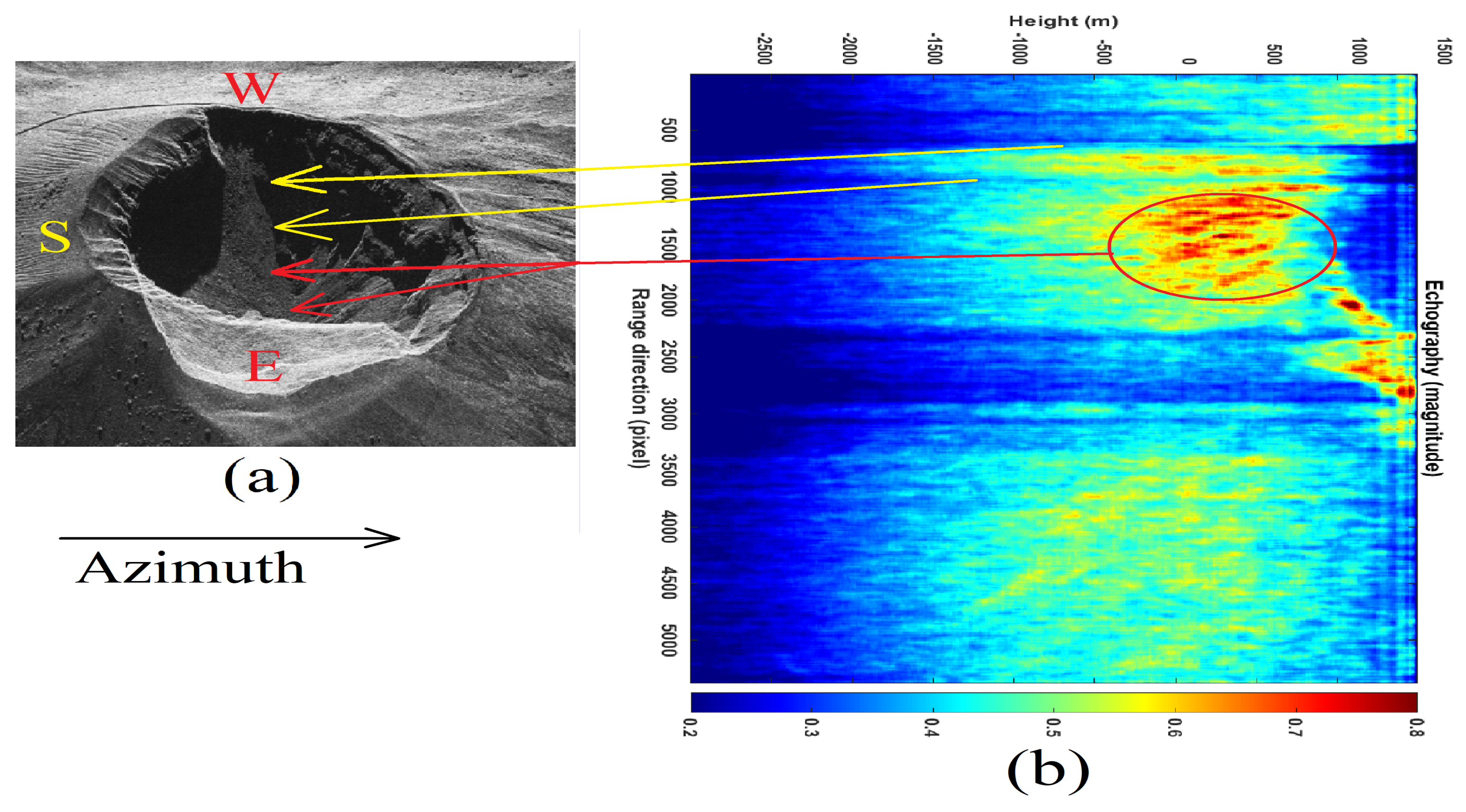
In this section, all the experimental results are described by processing a SAR image acquired by the COSMO-SkyMed Second Generation (CSG) satellite constellation. The data concerns a spotlight-2A acquisition mode, in the horizontal–horizontal (HH) polarization, with a Doppler band of about 22.5 kHz, and a chirp band of about 450 MHz. For this first case study, both the optical and the SLC image in magnitude are depicted in Figure 5a,b, respectively. The characteristics of the employed SAR image are listed in Table 1. Figure 6a is the representation of the SAR (magnitude) image where Vesuvius with its main crater is visible. Yellow line 1 is where the seismic tomogram is calculated. The test dataset is constituted by an entire range line belonging between the near range and the far range of the SAR image. Figure 6b is the result representing the estimated seismic tomography. The depth of investigation is about 3 km. In the figure, the surface topography of the volcano and its entire interior are visible. From the tomogram, it is possible to observe the crater of the main conduit inside red box 1. From this result, we observe the presence of vibration energy accumulations located in depth. This discontinuity suggests the presence of material that vibrates more concerning the background. This anomaly could be associated with the presence of denser material, and therefore with a sort of cap located below the main crater of Vesuvius. On the left side of the cap, there are two ducts, probably created by the pressure of the vapors or fluid gasses coming from underground. The maximum depth measured by the tomogram is approximately 3 km from the maximum topographic surface height of the volcano. Figure 6a,b is a detailed analysis of the of the volcano feeder conduit. In this figure, two apertures, probably excavated by high-pressure magmatic fluid gases, and the presence of a large portion of a denser material (having higher vibrational energy), residing below the surface of the main crater at a depth of about 1 km, are visible.
Figure 7a shows the SAR image (in magnitude) of Vesuvius according to a new tomographic line inserted, slightly more inclined, to cover as much as possible, in radar visibility, the volcano crater diameter, on the condition of having the greater scattering energy. On those pixels, we calculated the seismic tomogram visible in Figure 7b. In this case, the possible presence of a cap constituted by dense rocky material and the presence of an energetic gap where the seismic waves oscillate with less intensity is visible.
Figure 8a represents the SAR SLC image where the tomographic line 1 is shown where we investigate the acoustic response in depth. The result obtained, thus the tomography of the entire line is proposed in Figure 8b. The topographic height is correctly detected through line 2.
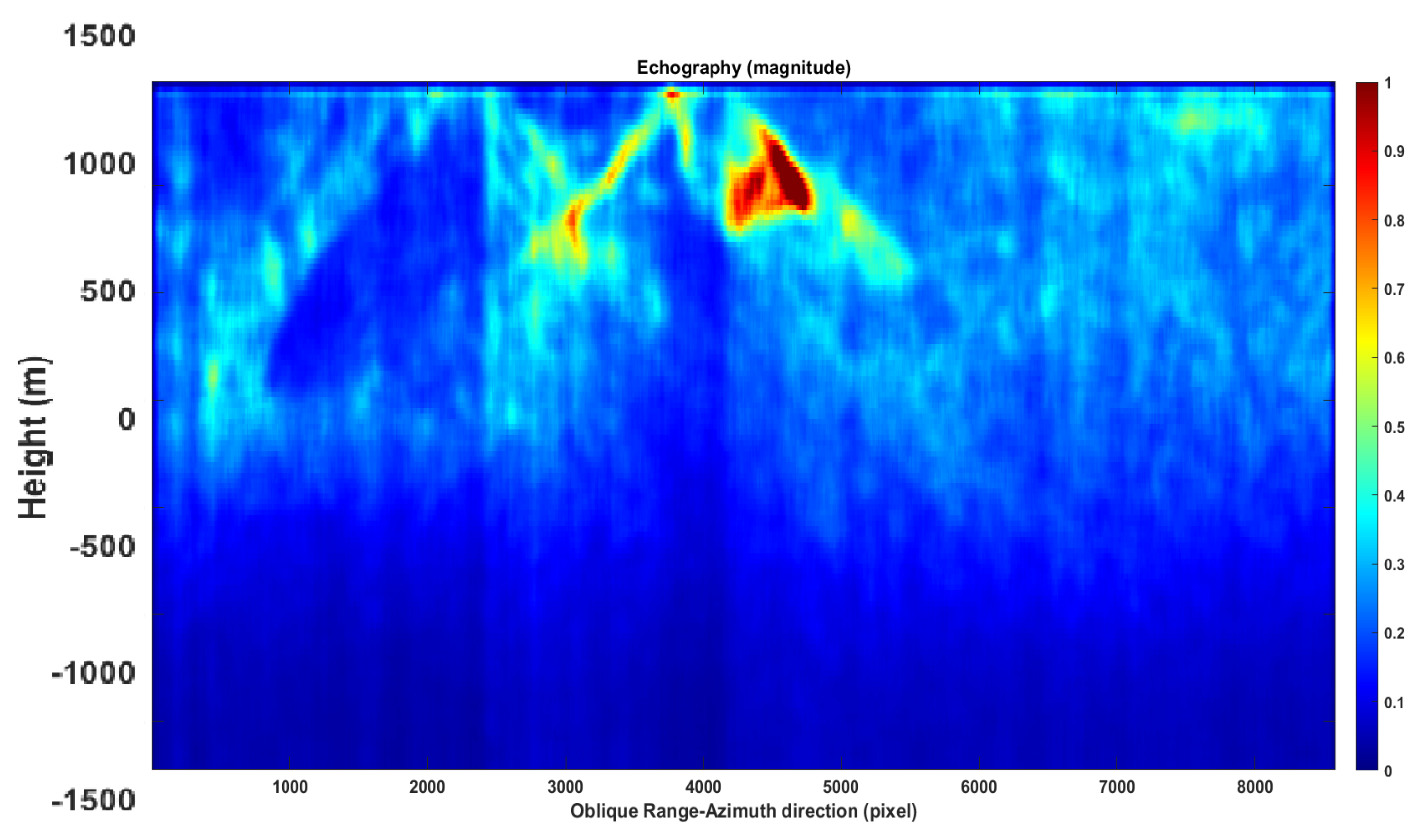
In Figure 9a, the detailed seismic tomography of the Vesuvius crater is depicted (particolar of box numer 1 of Figure 8b), and details of the SAR image are proposed in Figure 9b. Figure 9c is the sonic tomogram of a range line spanning the entire crater. Through yellow arrows 3 and 4, pointing to the SAR image, two conduits are shown; finally, through arrow 4, the presence of a massive debris accumulation is detected. This facility appears to be composed of several layers having different physical compositions. The debris layers are detailed within circle 1 (visible in Figure 9b). The maximum depth of the layers is measured to be about 2 km deep, relative to the top surface of the volcano. Figure 10 is an overview of Vesuvius for which the seismic tomogram has been calculated through a purely azimuth-oriented line, which is visible in Figure 10a, and tracked through yellow line 1. The tomographic result is shown in Figure 10b, for which the main section is shown within the red circle visible in Figure 10a. The result shows probable magmatic fluid conduits, detected in terms of vibrational energy discontinuities. Figure 11 represents the tomographic result obtained considering an oblique section, visible in Figure 11a. For this case, the tomographic line is traced through yellow line 1. The proposed tomographic map shows the entire volcano internal section (Figure 11b). The tomogram was calculated at a higher resolution and taking into account a longer orbital variation.
The following information is obtained from the calculated tomograms:
- The inner western volcano crater tomographic slopes consist of layered material, visible within yellow circle 1 of Figure 9b;
- The main volcano crater can be plugged by a cap of material consistent with vibration energy singularity, depicted within the yellow circle 2 of Figure 11b;
- The main conduits from the magma chamber rise from the east and west tomographic sections, indicated by arrows 3 and 4 of Figure 11b;
- The same results are obtained by calculating the sonic tomogram at a lower vibrational frequency, for which the result is visible in Figure 12.
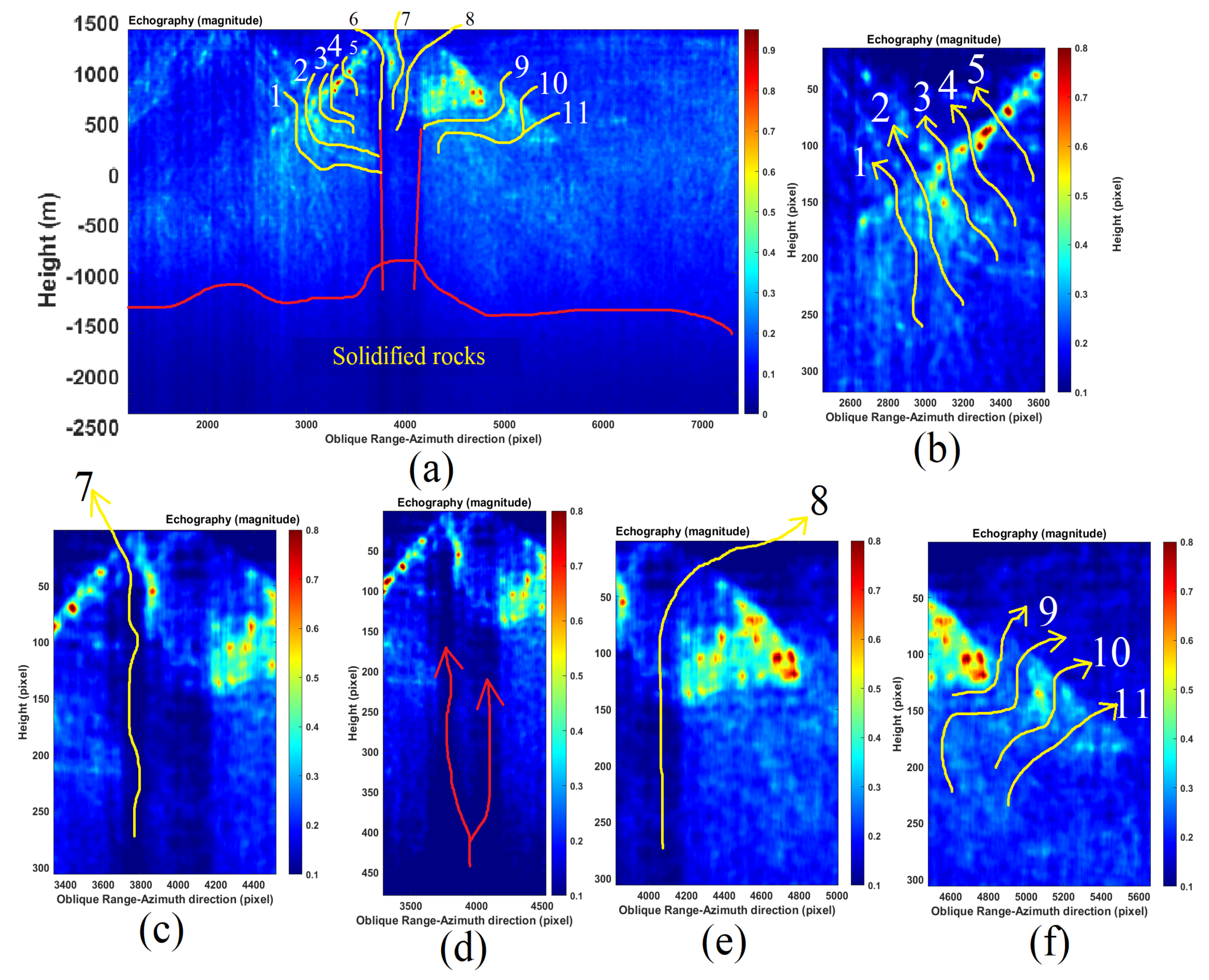
A detailed list of feeder conduits is proposed in Figure 13. These natural passages are made of material that does not resonate. We consider this characteristic as possible magmatic fluid paths that a hypothetical new eruption might prefer. From the western side of the great crater, it is possible to edit 11 fractures. The ones belonging from 1 through 5 are located within the main crater, while fractures 9–11 may extend outside the crater. The complete list of possible magmatic fluid paths can be seen in Figure 13a. A detailed tomographic section of the fractures finishing inside the crater can be seen in Figure 13b, while a detailed tomogram of the upper magmatic fluid ducts is visible in Figure 13c–e, and finally some external magmatic fluid paths are depicted in Figure 13f.
4. Validation of the Sonic Tomographic SAR Results
4.1. Topographic Validation
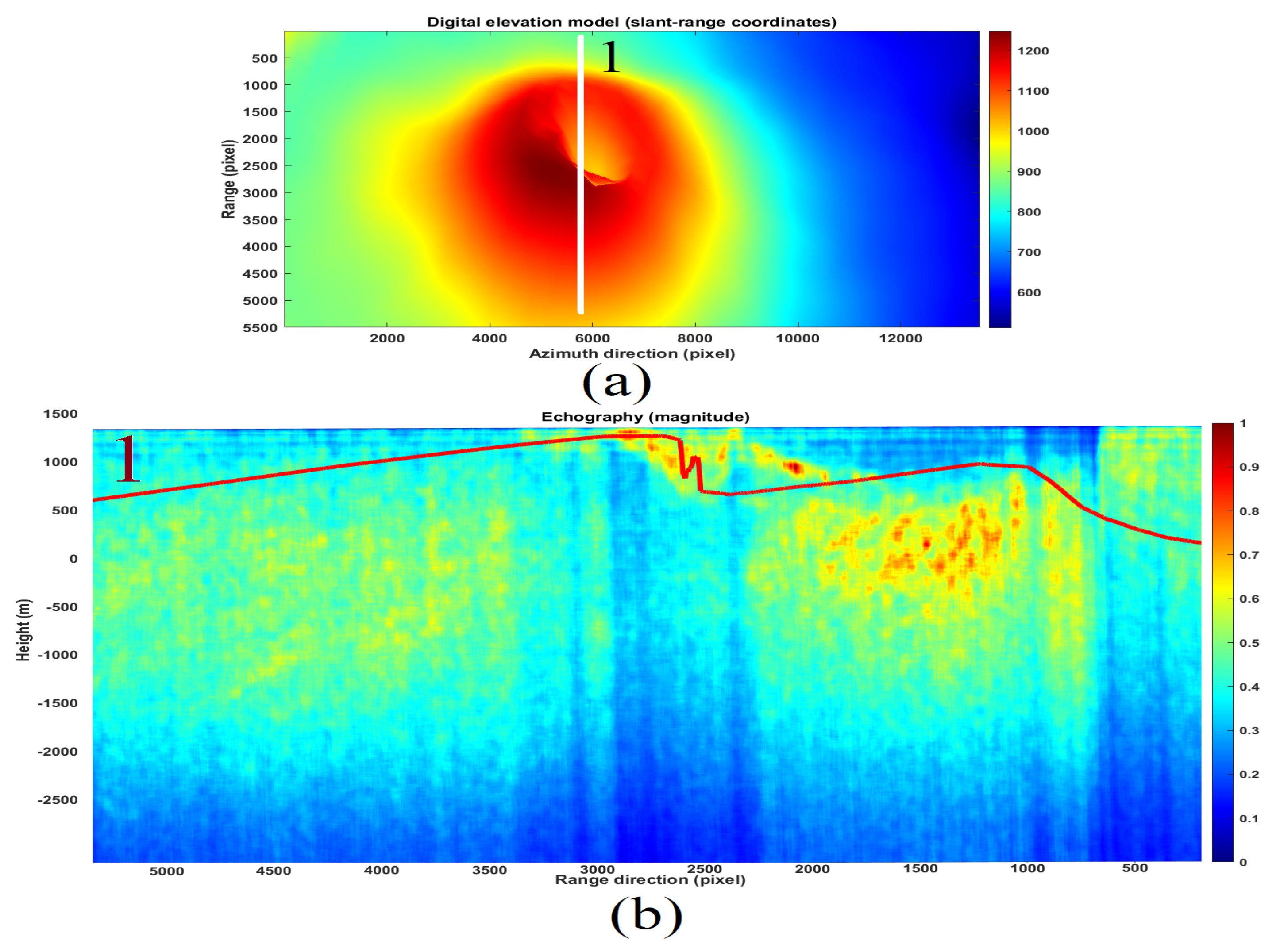
In this section, the topographic validation of the estimated tomograms is performed. The topographic elevation lines are provided by the digital elevation model (DEM) generated by the Shuttle Radar Topography Mission (SRTM). The topographic lines are superimposed on the estimated tomographic sections. In this specific case, the topographic line 1 visible in Figure 14a has been extrapolated from the global SRTM topographic surface, which is coincident with the tomographic line 1 shown in Figure 11a. The topographic line has been merged on the tomogram and the total information is visible in Figure 15b. The visual analysis shows the surface tomogram overlapping almost perfectly with the topographic line, which is represented by yellow line 1.
The next validation case is to compare the position of the topographic line 1 visible in Figure 16a (always extrapolated from the SRTM-DEM) with the top of the tomography coincident to line 1 shown in Figure 8a and the consequent merged information is visible in Figure 15b. The visual analysis shows the almost perfect overlap of the superficial component of the tomogram with the topographic line, which is represented by yellow line 1. The last performance analysis case study is shown in Figure 14a,b. For this case, the tomographic line is perfectly oriented along the range direction. The objective was to study the tomographic reconstruction robustness under heavy foreshortening and layover effects. The tomographic picture is reported in Figure 14b. In this case, the eastern side of the crater (the one characterized by layover) is better seen than the western side (the one characterized by foreshortening). However, possible magmatic fluid conduits communicating with both the inner and outer parts of the main volcano cone remain visible on the eastern side of the crater. The tomogram has been divided into three portions: result numbers 2, 3, and 4, which are compartmentalized by three red squares visible in Figure 14b. Each tomographic surface is pointed at its tomographic line reference, which is visible in Figure 14a. The portion of the tomogram characterized by layover is number 2, while result number 3 is the one representing the interior of the main crater. Finally, result number 4 refers to the descending side of the volcanic cone. Results confirm the presence of vibratory material, similar to rock, probably composed of cooled compact solidified magma that produces a substantial blockage mass located deeply inside the main volcanic conduit. This blockage is visible within box 5 of Figure 14b.
4.2. Vibration Validation
Vibrational validation is carried out by comparing data estimated by the satellite with those observed by the "in situ" seismological stations installed at Vesuvius. In situ data are provided in open source from the Italian National Institute of Geophysics and Volcanology (INGV), and are downloadable from the following website: https://eida.ingv.it/it/, accessed on 23 April 2022. In this context, the vibrational data estimated by the satellite and those provided by the seismic in situ stations listed in Table 2 are synchronized in space and time.
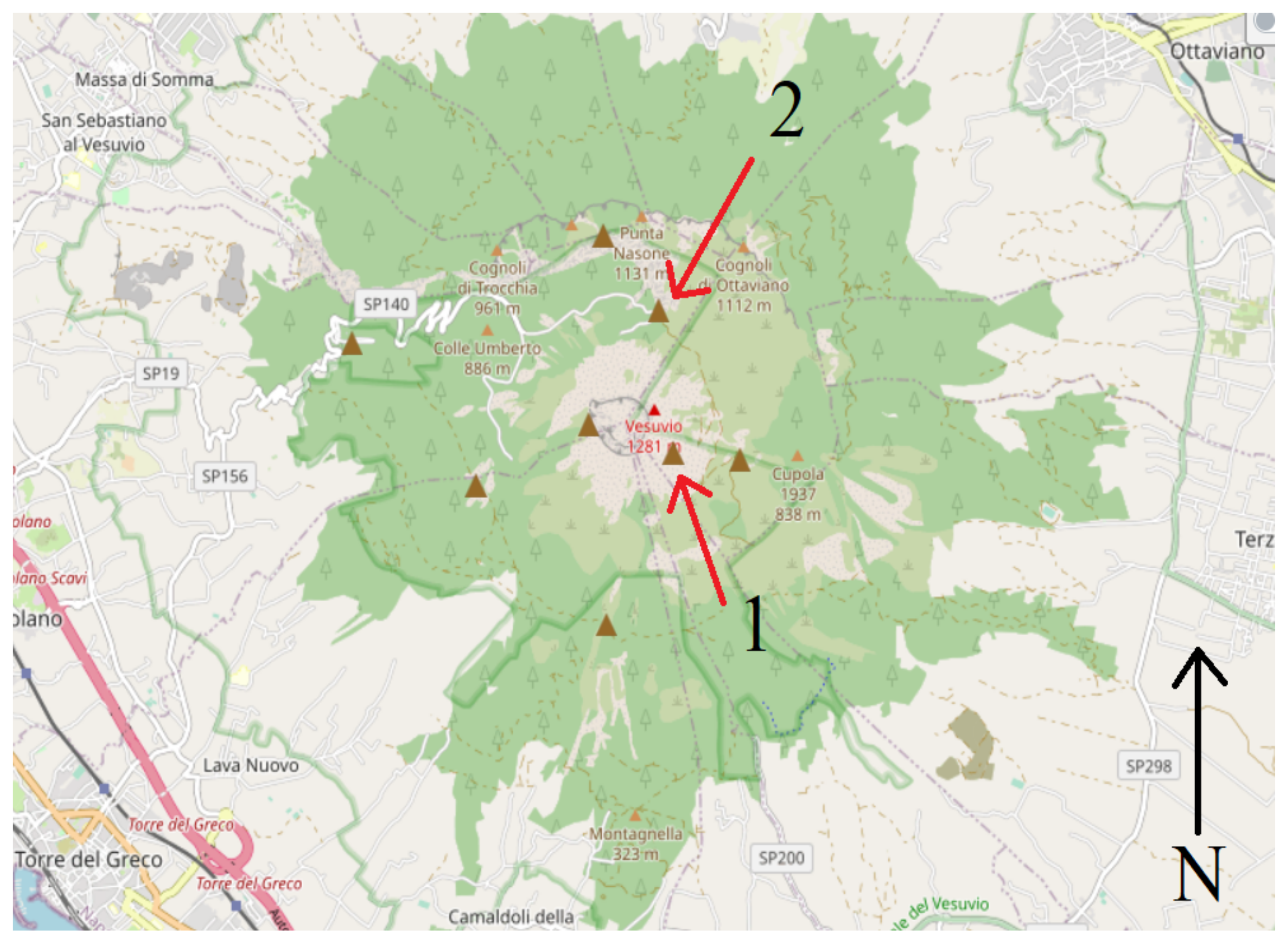
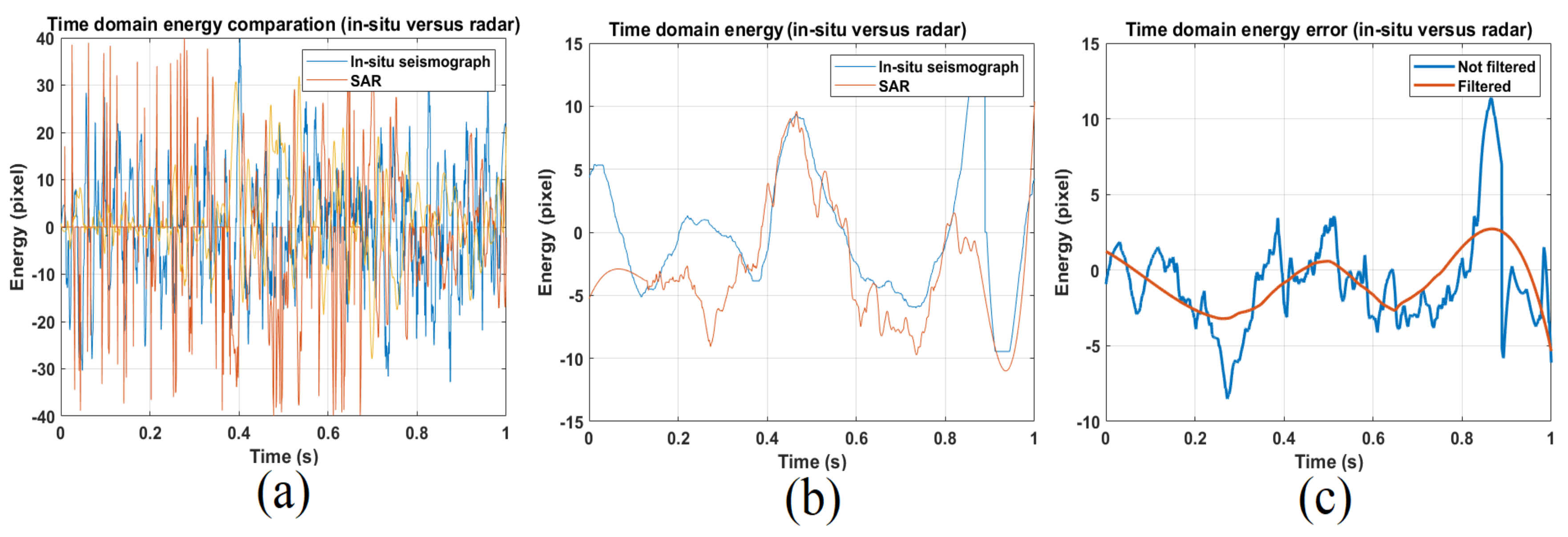
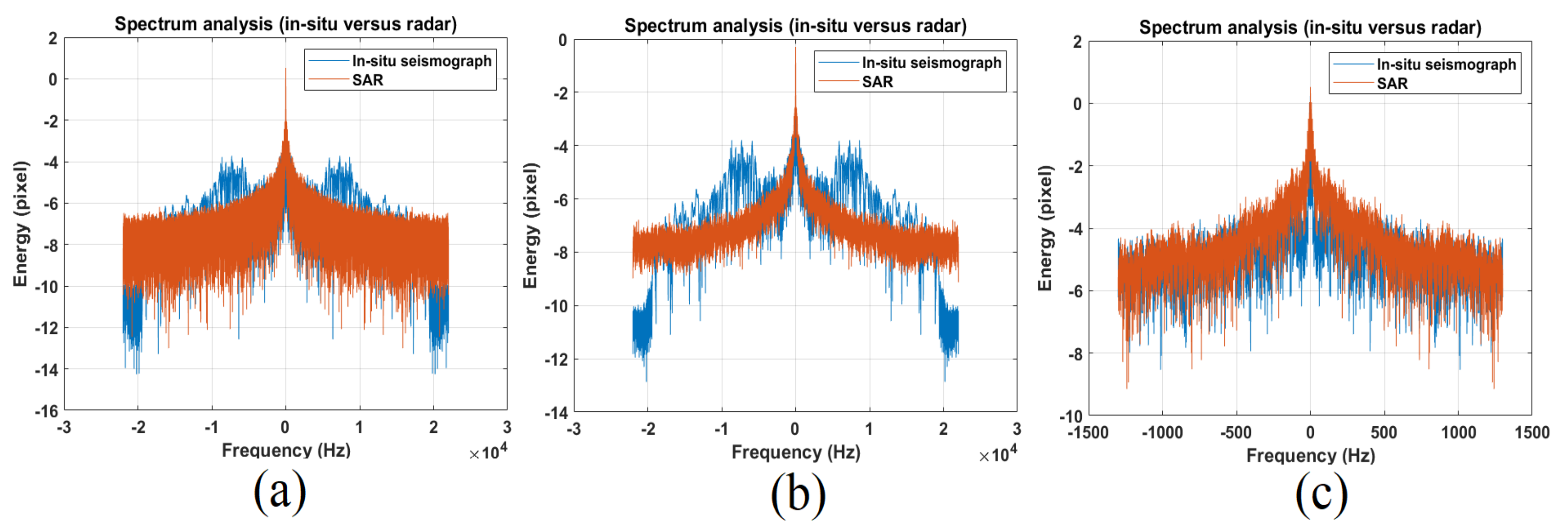
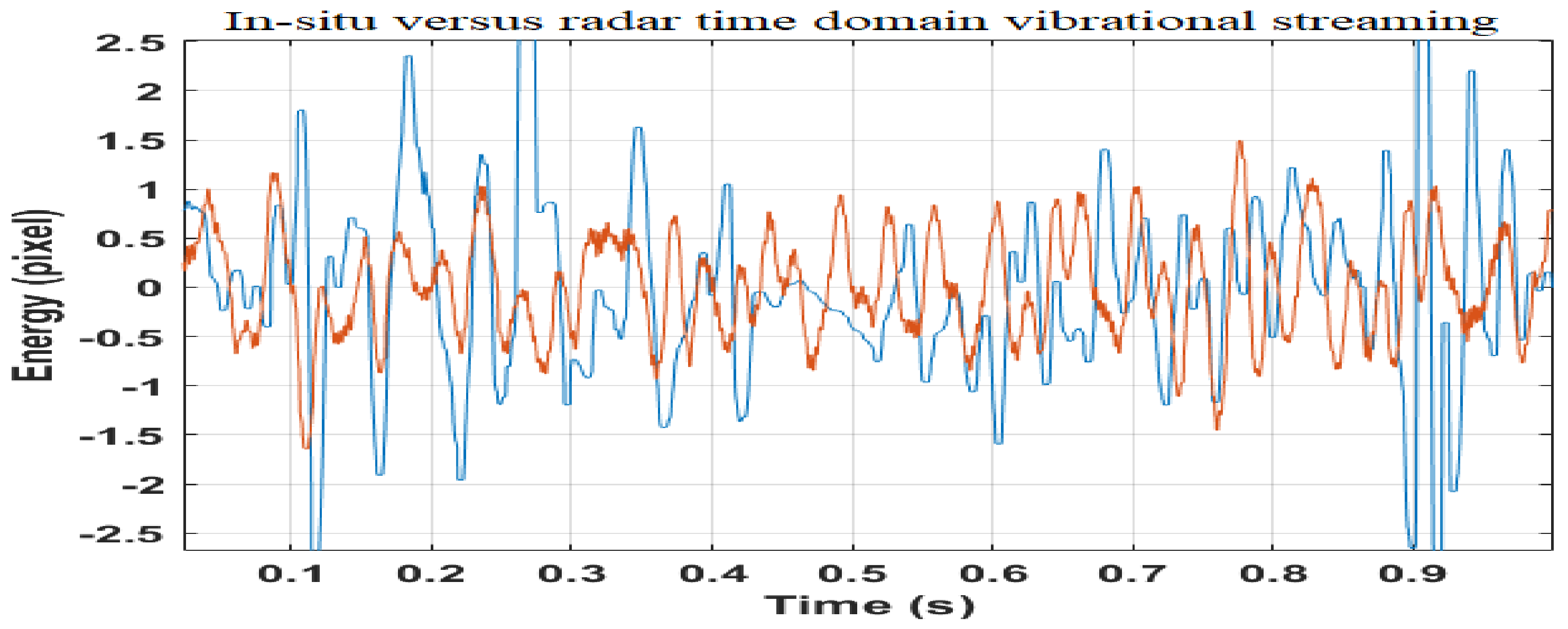
Figure 17 shows the map where the Vesuvius seismic stations are located. IV-VCRE and VBKN in situ station data are considered in this stage and are the only ones compatible with line-of-sight radar visibility. All other measurement stations were either not visible or were located outside the SAR imaging scene. Figure 18a,b and Figure 19a,b represent the optical and radar observations, respectively, of the seismographic stations. The first facility is located at the east side of the crater and the second one is installed toward the northern side. The two stations are successfully represented on both the optical and radar images (indicated both by arrows number 1). In Figure 20a–c, the vibrational spectrum streaming recorded by the IV-VCRE seismographic station, superimposed to the respective spectrogram recorded by radar, is depicted. Figure 20a represents the unfiltered full-bandwidth spectrum, while Figure 20b is the filtered spectrum; finally Figure 20c represents a narrowed detail spectrum at approximately 1 kHz of bandwidth. The blue color function is that of the “in situ” station, while the brown color function is the radar-estimated vibrational spectrum. The native time trend (1 s of synchronized streaming) is shown in Figure 21a. The filtered time-domain plot (approximately composed of 1-s wide synchronized data streaming) is reported in Figure 21b, finally the IV-VCRE in situ station versus SAR vibrational streaming measurement errors is proposed in Figure 21c. The blue function represents the unfiltered error, while the one in brown is the filtered error. It can be seen that this error, while oscillating around zero, remains confined to very low values. In Figure 22a–c, the spectrum of the vibrational streaming recorded by the IV-VBKN seismographic station is represented. Figure 22a represents the spectrum in its entirety, Figure 22b is the filtered spectrum, while Figure 22c represents a narrowed detail dataset at approximately 1 kHz of bandwidth. Also, in this case the blu and the brown functions are the in situ and the radar estimated vibrational spectrum, respectively. The unfiltered time-domain sampled vibrations (approximately 1-s synchronized streaming) are shown in Figure 23. Although it is very difficult to perfectly synchronize two different measurement instruments—the first one is located on the ground, while the second one is located in space—such time synchronization turns out to be very acceptable. Both instruments measure the seismic background of the area. This result brings the SAR’s effective measurement accuracy to attention.
4.3. Tomographic Validation
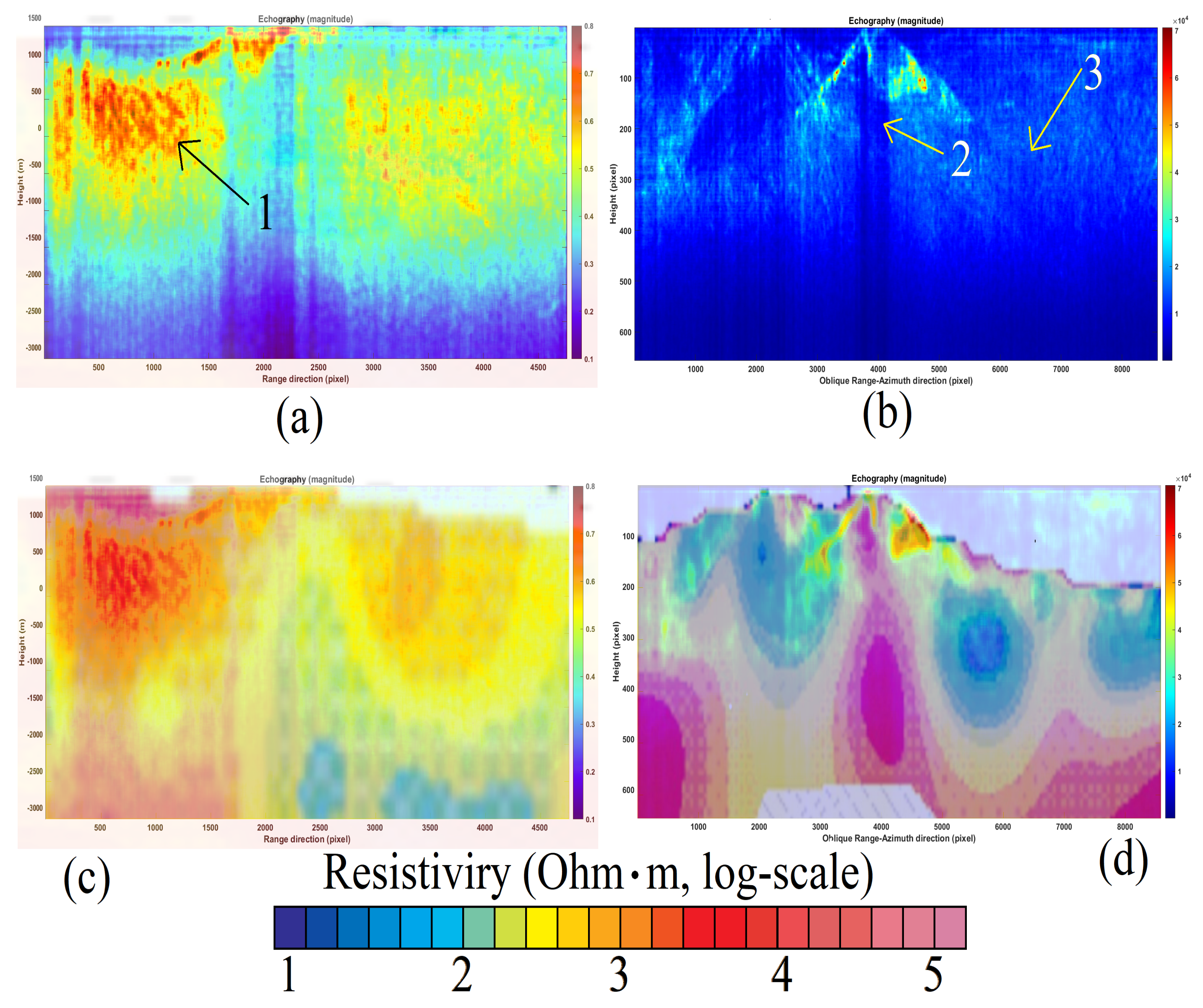
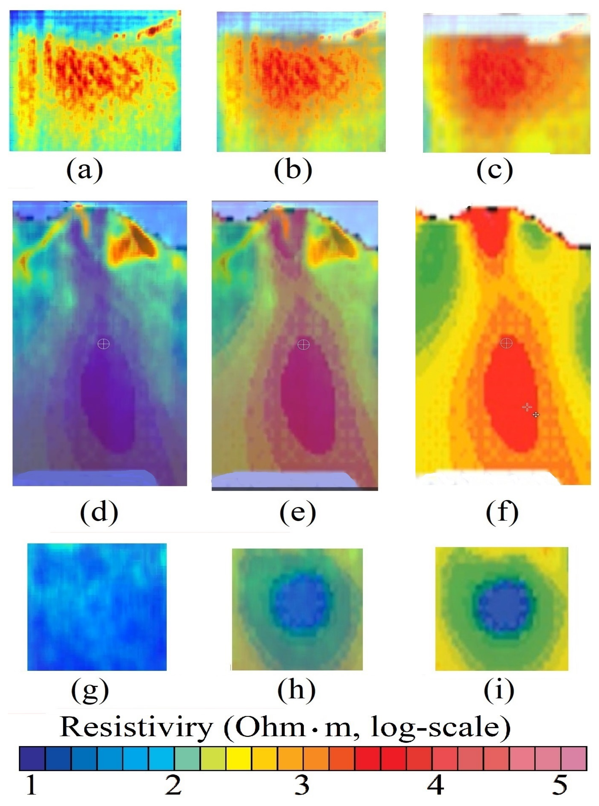
In this section, the comparison of data estimated through magnetotelluric tomography with those estimated through SAR tomography is evaluated. Successively, the visual comparison relates the magnitude of the earthquakes that occurred during the month, within which the SAR observation is made. The estimated tomographic planes found the perfect overlap of the estimated results with the radar. In Figure 24a–d, we report the radar-estimated tomographic maps superimposed on the magnetotelluric tomography results. More precisely, Figure 24a is the in-range SAR tomography; Figure 24c is the superposition of Figure 24a radar tomography with magnetotelluric tomography. On the other hand, Figure 24b shows the range-azimuth oblique SAR tomography, while Figure 24c is the superposition of the oblique radar tomography in Figure 24b with the magnetotelluric tomography. In Figure 25a,i, some details are depicted to better show the existing tomographic overlay. The images in Figure 25a–c refer to the topographic detail of Figure 24a, where a reference area is indicated by arrow number 1. Figure 25a is the radar data alone, Figure 25b is the 50% overlay of the radar data on the magnetotelluric tomography, and finally Figure 25c is the magnetotelluric tomography map shown alone. The images of Figure 25d–f refer to the tomographic detail of Figure 24b, indicated by arrow 2. Figure 25d is the radar data alone, Figure 25e is the 50% overlay of the radar data with the magnetotelluric tomography, and finally Figure 25f is the magnetotelluric tomography, again shown alone.
Finally, the images of Figure 25g–i refer to the tomographic detail of Figure 24b, indicated by arrow 3. Figure 25g is the radar data alone, Figure 25h is the 50% overlay of the radar data with the magnetotelluric tomography, and finally Figure 25i is the magnetotelluric tomography without any overlay. The comparative assessment formed by the visual validation between the results estimated through the seismic sensors network installed in the proximity of Vesuvius and measured satellite results are secondly performed. The data were extrapolated from the public and institutional websites of the INGV. In this context, the seismic values map is shown in Figure 26, and is correlated to the SAR tomographic results of Figure 14b. In the Figure, blue and colored circles represent some seismic events. The center of each point is placed in the 3D space on which the source of the seismic event was measured, while the radius of each circle measures its magnitude. The Figure also contains the magnitude legend and four scales can be distinguished, the number 0 value represents all seismic events between 0 and 1 Richter scale magnitude. Number 1 represents all events of magnitude between 1 and 2, circle 2 between 2 and 3, and finally, the largest circle is the number 3, which represents all seismic events greater than 3 degrees of magnitude on the Richter scale. The blue circles represent seismic events that occurred throughout January 2022, while the red color represents only those seismic events that occurred in February 2022, which is the month in which the SAR data was acquired. From a visual comparison, we keep a good correspondence of the data if compared to the one estimated through SAR tomography. It is clear that the temporal correspondence of the SAR acquisition which consists of a few seconds is not comparable with the large temporal duration of the measurements made through the “in situ” sensors, but we find a good correlation between the red seismic events that coincide very much in space with the magmatic consistency estimated through the SAR seismic tomography. The depth also coincides greatly.
5. Discussion
This is the first time that a SAR has been employed to estimate the consistency of depth structures, down to 3 km, considering also that the observations are performed from space. This preliminary work may pave the way for a new type of radar exploitation, where the carrier physical phenomenon is formed by coherent electromagnetic X-band transmissions and azimuth focusing made using ad hoc designed matched filters tuned at the zero Doppler. This procedure can grab phononic (intended to be the vibration of matter) physical parameters. In this context, photons are used as a carrier medium that contains phononic information as well. It seems that this system, although still to be improved and refined, works. This technique can be extended to maybe detect crude oil, or natural gas underground pockets, to quickly search for veins in metals and rare earth, or to assess the consistency of the matter from which all the world’s great infrastructures are made. In the present work, we first thought about both nature and humanity preservation, and then found a method (which at present remains unresolved), namely that of looking inside volcanoes with high-resolution imaging from space. It seemed natural to us to focus our research on one of the world’s most dangerous volcanoes. It is located in Italy in the middle of the highly populated city of Naples, Vesuvius. In addition, this technique allows the construction of an accurate and truthful model of the Earth’s subsurface. This possibility appears very important and could serve in helping to strengthen predictive models useful in both the volcanological and seismological fields. According to [34], there is an electromagnetic interaction with the atmosphere. The technique employs the single SAR image, acquired in a time of about 14 s; surely there is an electromagnetic phase delay due to the atmosphere. However, this delay, in practice, does not affect the correct estimation of the tomography, as it is constant in time (this effect is assumed to be time-invariant), so we assume that atmospheric delay remains constant within the SAR acquisition. However, the proposed technique is very robust in terms of compensating for atmospheric interaction as we scan in the Doppler domain, within the single SAR image. To this end, MCA of atmospheric issues is fully described and solved in [28]. Concluding, the proposed technique, can be considered a potential “gap-filler”, thus allowing us to look inside rigid bodies, like volcanoes, even over high spatial resolution. Authors employed specifically designed software for processing tomographic slices. At the present, there is no commercial software capable of extracting the phonon information embedded in the SAR data. The authors are available in collaborating with other research groups for reproducing the proposed tomographic method specifically, for all those sites that need to be studied in depth.
6. Conclusions
This work describes an imaging method based on the analysis of micro-motions present on volcanoes and generated by underground Earth tremors. We showed a series of tomographic maps representing the internal echography of volcanoes. Processing the coherent vibrational information present on the single SAR image, in the single-look-complex configuration, we exploited the sound information penetrating tomographic imaging over a depth of about 3 km from the Earth’s surface. The experimental results were calculated processing an SLC image from the COSMO-SkyMed Second Generation satellite constellation of the Italian volcano Vesuvius. Tomographic maps revealed the presence of the solidified magma, and the main and the secondary feeder conduit. In addition, both the main and secondary fractures are visible. Concluding, we also declare that although the results of the considered case study are promising, they should be confirmed by using other case studies in the future.
Funding
This research received no external funding.
Data Availability Statement
Data used for this work can be requested at https://www.e-geos.it/ or at https://www.asi.it/ (accessed on 1 April 2022).
Acknowledgments
We would like to thank Daniele Perissin for making the SARPROZ software available, through which many calculations were carried out more easily and quickly. We also thank the Italian Space Agency for providing the SAR data. The in situ seismic numerical data were kindly provided by the Italian Institute of Geophysics and Volcanology (INGV), which can be downloaded from the website: https://eida.ingv.it/it/ (accessed on 23 April 2022). Finally, We thank Corrado Malanga, Professor of Industrial Chemistry at the Faculty of Chemistry, University of Pisa (Italy), for guiding me in formulating the idea of extrapolating phononic information through photonic processing of SAR data. (https://corradomalangaexperience.com/, accessed on 1 January 2022).
Conflicts of Interest
The author declare no conflict of interest.
Appendix A. Mathematical Formulation
Appendix A.1. Doppler Sub-Apertures Model
The SAR data belonging to the electromagnetic image are formed through the focusing process that involves the application of a two-dimensional matched filter acting in the range direction and in the azimuth direction. The SLC signal resulting from compression is given by [35]:
Equation (A1) represents the focused SAR signal generated by the back-scattered electromagnetic energy of a point target supposed to be stationary. The parameter is the SAR radio-frequency wavelength. The terms , and are the total chirp and Doppler bandwidths respectively. The total synthetic aperture is equal to and the azimuth resolution . In (A1) the parameter identifies the position in range where the maximum of the sinc function is positioned, while in azimuth it is centered around ”zero”. In the case where the peak of the sinc function has a nonzero coordinate along the azimuth dimension, Equation (A1) can be recast as:
in (A2) , and are the slant-range, azimuth position of the single-target beam center, into the image coordinates. In this context the DFT is equal to:
which has a rectangular shape. In (A3) the parameter DFT2 is the two-dimensional digital Fourier transform.
Appendix A.2. Doppler Sub-Apertures Model
In this paper author tests a strategy that employs Doppler sub-apertures, that are generated to measure target motion. Figure 2 represents the used bandwidth allocation strategy. From the single SAR image We calculate the DFT2 which, according to (A3), has a rectangular shape. As can be seen from Figure 2, is the total Doppler band synthesized with the SAR observation, while is the bandwidth not processed from the matched-filter boundaries, to obtain a sufficient sensitivity to estimate target motions. In this context formula (A3) is the focused SAR spectrum, at maximum resolution, thus exploiting the whole band , in accordance with the frequency allocation strategy shown in Figure 2, the following range-Doppler sub-apertures large-matrix is constructed for the Master multi-dimensional information:
and for the slave, the following large-matrix is presented:
The explanation of the chirp-Doppler sub-aperture strategy, represented in Figure 2 is the following: In Figure 2, master and slave sub-bands are generated by focusing the SAR image, where the matched-filter is set to exploit a range-azimuth bandwidth equal to . The not-processed bandwidths are divided into equally-distributed bandwidths steps respectively. At this point rigid shifts of the master–slave system are made along the azimuth bandwidth domain, this is made to populate the entire row of Equations (A4), and (A5). The process is repeated times for each shift in azimuth, in fact, Figure 2 (1), (2), and (3), represent the azimuth frequency variation strategy when the Doppler bandwidth is located at . At each Doppler frequency shift every element of (A4), and (A5) is populated.
Appendix A.3. Doppler Sub-Aperture Strategy
The decomposition of the SAR data into Doppler sub apertures is formalized in this subsection, which is performed starting from the spectral representation of the focused SAR data. To this end, notice that the generic th chirp sub-aperture 2-dimensional DFT of (A2) is given by:
from the last equation, it turns out that a single point stationary target has a two-dimensional rectangular nature with total length proportional to the range-azimuth bandwidths respectively. The phase term is due to the sinc function dislocation in range and azimuth when the SLC SAR data are considered. In the SAR, the movement of a point target with velocity in both range and azimuth direction is immediately warned by the focusing process, resulting in the following anomalies:
- azimuth displacement in the presence of target constant range velocity;
- azimuth smearing in the presence of target azimuth velocity or target range accelerations;
- range-walking phenomenon, visible as range defocusing, in the presence of target range speed, backscattered energy can be detected over one or more range resolution cells.
In practical cases, the backscattered energy from moving targets is distributed over several range-azimuth resolution cells. As a matter of fact, considering the point-like target (of Figure 1) that is moving with velocity whose range-azimuth and acceleration components are , and , respectively, then it is possible to highlight
considering the following Taylor expansion:
and that , and , (A7) can be written in the following form:
the term can be neglected and by approximating Equation (A10) can be written like:
recasting (A11) in terms of , We obtain [32]:
where:
- (due to range velocity);
- (due to range acceleration);
- (due to azimuth velocity).
References
- Moe, N.J. The View from Vesuvius; University of California Press: Berkeley, CA, USA, 2002. [Google Scholar]
- Sigurdsson, H.; Cashdollar, S.; Sparks, S.R. The eruption of Vesuvius in AD 79: Reconstruction from historical and volcanological evidence. Am. J. Archaeol. 1982, 86, 39–51. [Google Scholar] [CrossRef] [Green Version]
- Papale, P.; Dobran, F. Modeling of the ascent of magma during the plinian eruption of Vesuvius in AD 79. J. Volcanol. Geotherm. Res. 1993, 58, 101–132. [Google Scholar] [CrossRef]
- Santacroce, R. A general model for the behavior of the Somma-Vesuvius volcanic complex. J. Volcanol. Geotherm. Res. 1983, 17, 237–248. [Google Scholar] [CrossRef]
- Auger, E.; Gasparini, P.; Virieux, J.; Zollo, A. Seismic evidence of an extended magmatic sill under Mt. Vesuvius. Science 2001, 294, 1510–1512. [Google Scholar] [CrossRef] [PubMed]
- De Natale, G.; Troise, C.; Trigila, R.; Dolfi, D.; Chiarabba, C. Seismicity and 3-D substructure at Somma–Vesuvius volcano: Evidence for magma quenching. Earth Planet. Sci. Lett. 2004, 221, 181–196. [Google Scholar] [CrossRef]
- De Lorenzo, S.; Di Renzo, V.; Civetta, L.; D’antonio, M.; Gasparini, P. Thermal model of the Vesuvius magma chamber. Geophys. Res. Lett. 2006, 33, 16. [Google Scholar] [CrossRef]
- Zuccaro, G.; Cacace, F.; Spence, R.; Baxter, P. Impact of explosive eruption scenarios at Vesuvius. J. Volcanol. Geotherm. Res. 2008, 178, 416–453. [Google Scholar] [CrossRef]
- Benkhelifa, M.; Gindre, M.; Le Huerou, J.Y.; Urbach, W. Echography using correlation techniques: Choice of coding signal. IEEE Trans. Ultrason. Ferroelectr. Freq. Control. 1994, 41, 579–587. [Google Scholar] [CrossRef]
- Carotenuto, R.; Caliano, G.; Caronti, A.; Savoia, A.; Pappalardo, M. Fast scanning probe for ophthalmic echography using an ultrasound motor. IEEE Trans. Ultrason. Ferroelectr. Freq. Control. 2005, 52, 2039–2046. [Google Scholar] [CrossRef]
- Matani, A.; Shigeno, T. Phase series echography with prior waveform distortion for evaluating posterior waveform distortion. IEEE Trans. Ultrason. Ferroelectr. Freq. Control. 2006, 53, 2019–2025. [Google Scholar] [CrossRef]
- Anantrasirichai, N.; Hayes, W.; Allinovi, M.; Bull, D.; Achim, A. Line detection as an inverse problem: Application to lung ultrasound imaging. IEEE Trans. Med. Imaging 2017, 36, 2045–2056. [Google Scholar] [CrossRef] [Green Version]
- Demi, L.; Demi, M.; Prediletto, R.; Soldati, G. Real-time multi-frequency ultrasound imaging for quantitative lung ultrasound–first clinical results. J. Acoust. Soc. Am. 2020, 148, 998–1006. [Google Scholar] [CrossRef]
- Berryman, J.G. Weighted least-squares criteria for seismic traveltime tomography. IEEE Trans. Geosci. Remote. Sens. 1989, 27, 302–309. [Google Scholar] [CrossRef]
- Song, L.p.; Zhang, S.y. Singular value decomposition-based reconstruction algorithm for seismic traveltime tomography. IEEE Trans. Image Process. 1999, 8, 1152–1154. [Google Scholar] [CrossRef]
- Shapiro, N.M.; Campillo, M.; Stehly, L.; Ritzwoller, M.H. High-resolution surface-wave tomography from ambient seismic noise. Science 2005, 307, 1615–1618. [Google Scholar] [CrossRef] [Green Version]
- Brenguier, F.; Shapiro, N.M.; Campillo, M.; Ferrazzini, V.; Duputel, Z.; Coutant, O.; Nercessian, A. Towards forecasting volcanic eruptions using seismic noise. Nat. Geosci. 2008, 1, 126–130. [Google Scholar] [CrossRef] [Green Version]
- Devaney, A. Geophysical diffraction tomography. IEEE Trans. Geosci. Remote. Sens. 1984, 1, 3–13. [Google Scholar] [CrossRef]
- Witten, A.J.; Long, E. Shallow applications of geophysical diffraction tomography. IEEE Trans. Geosci. Remote. Sens. 1986, 24, 654–662. [Google Scholar] [CrossRef]
- Paulatto, M.; Minshull, T.; Baptie, B.; Dean, S.; Hammond, J.O.; Henstock, T.; Kenedi, C.; Kiddle, E.; Malin, P.; Peirce, C.; et al. Upper crustal structure of an active volcano from refraction/reflection tomography, Montserrat, Lesser Antilles. Geophys. J. Int. 2010, 180, 685–696. [Google Scholar] [CrossRef] [Green Version]
- Liu, Z.; Chatzidakis, S.; Scaglione, J.M.; Liao, C.; Yang, H.; Hayward, J.P. Muon tracing and image reconstruction algorithms for cosmic ray muon computed tomography. IEEE Trans. Image Process. 2018, 28, 426–435. [Google Scholar] [CrossRef]
- Sherburn, S.; White, R.S.; Chadwick, M. Three-dimensional tomographic imaging of the Taranaki volcanoes, New Zealand. Geophys. J. Int. 2006, 166, 957–969. [Google Scholar] [CrossRef] [Green Version]
- Lee, S.J.; Kim, S.; Rhie, J.; Kang, T.S.; Kim, Y. Upper crustal shear wave velocity and radial anisotropy beneath Jeju Island volcanoes from ambient noise tomography. Geophys. J. Int. 2021, 225, 1332–1348. [Google Scholar] [CrossRef]
- Yudistira, T.; Métaxian, J.P.; Putriastuti, M.; Widiyantoro, S.; Rawlinson, N.; Beauducel, F.; Zulfakriza, Z.; Nugraha, A.; Laurin, A.; Fahmi, A.; et al. Imaging of a magma system beneath the Merapi Volcano complex, Indonesia, using ambient seismic noise tomography. Geophys. J. Int. 2021, 226, 511–523. [Google Scholar] [CrossRef]
- Letort, J.; Roux, P.; Vandemeulebrouck, J.; Coutant, O.; Cros, E.; Wathelet, M.; Cardellini, C.; Avino, R. High-resolution shallow seismic tomography of a hydrothermal area: Application to the Solfatara, Pozzuoli. Geophys. J. Int. 2012, 189, 1725–1733. [Google Scholar] [CrossRef] [Green Version]
- Agostinetti, N.P.; Chiarabba, C. Seismic structure beneath Mt Vesuvius from receiver function analysis and local earthquakes tomography: Evidences for location and geometry of the magma chamber. Geophys. J. Int. 2008, 175, 1298–1308. [Google Scholar] [CrossRef]
- Troiano, A.; Petrillo, Z.; Di Giuseppe, M.G.; Balasco, M.; Diaferia, I.; Di Fiore, B.; Siniscalchi, A.; Patella, D. About the shallow resistivity structure of Vesuvius volcano. Ann. Geophys. 2008, 1, 1–10. [Google Scholar] [CrossRef]
- Biondi, F.; Addabbo, P.; Clemente, C.; Ullo, S.L.; Orlando, D. Monitoring of Critical Infrastructures by Micromotion Estimation: The Mosul Dam Destabilization. IEEE J. Sel. Top. Appl. Earth Obs. Remote. Sens. 2020, 13, 6337–6351. [Google Scholar] [CrossRef]
- Biondi, F.; Addabbo, P.; Ullo, S.L.; Clemente, C.; Orlando, D. Perspectives on the structural health monitoring of bridges by synthetic aperture radar. Remote. Sens. 2020, 12, 3852. [Google Scholar] [CrossRef]
- Biondi, F. COSMO-SkyMed staring spotlight SAR data for micro-motion and inclination angle estimation of ships by pixel tracking and convex optimization. Remote. Sens. 2019, 11, 766. [Google Scholar]
- Biondi, F.; Addabbo, P.; Orlando, D.; Clemente, C. Micro-motion estimation of maritime targets using pixel tracking in COSMO-SkyMed synthetic aperture radar data—An operative assessment. Remote. Sens. 2019, 11, 1637. [Google Scholar] [CrossRef] [Green Version]
- Raney, R.K. Synthetic Aperture Imaging Radar and Moving Targets. IEEE Trans. Aerosp. Electron. Syst. 1971, 3, 499–505. [Google Scholar] [CrossRef]
- Tufillaro, N.B. Nonlinear and chaotic string vibrations. Am. J. Phys. 1989, 57, 408–414. [Google Scholar] [CrossRef]
- Biondi, F.; Clemente, C.; Orlando, D. An Atmospheric Phase Screen Estimation Strategy Based on Multichromatic Analysis for Differential Interferometric Synthetic Aperture Radar. IEEE Trans. Geosci. Remote. Sens. 2019, 57, 7269–7280. [Google Scholar] [CrossRef]
- Curlander, J.C.; McDonough, R.N. Synthetic Aperture Radar: Systems and Signal Processing; Wiley: New York, NY, USA, 1991. [Google Scholar]
Figure 2.
Doppler sub-aperture strategy. (1) Spectrum explored from the beginning. (2) Spectrum explored from the middle. (3) Finally explored spectrum.
Figure 2.
Doppler sub-aperture strategy. (1) Spectrum explored from the beginning. (2) Spectrum explored from the middle. (3) Finally explored spectrum.

Figure 3.
Tomographic acquisition geometry. (a) Orbital geometry with the schematic representation of moving masses on the considered pixels. (b) Orbital geometry with the measured vibrations present on the considered pixels. (c) Details of the spring-mass scheme. (d) orthogonal baseline scheme for tomography.

Figure 4.
Computational scheme of tomographic imaging.

Figure 5.
Environment images. (a) optical image. (b) SLC SAR image in magniture.

Figure 6.
Range-line echographic tomography detailed result (magnitude). (a) SLC SAR image (in magnitude). (b) Tomographic result (in magnitude).
Figure 6.
Range-line echographic tomography detailed result (magnitude). (a) SLC SAR image (in magnitude). (b) Tomographic result (in magnitude).

Figure 7.
Range-line echographic tomography result (magnitude). (a) SLC SAR image (in magnitude). (b) Tomographic result (in magnitude).
Figure 7.
Range-line echographic tomography result (magnitude). (a) SLC SAR image (in magnitude). (b) Tomographic result (in magnitude).

Figure 8.
Range-line echographic tomography result (magnitude). (a) SLC SAR image (in magnitude). (b) Tomographic result (in magnitude). The yellow tomographic line is indicated by the number 1.
Figure 8.
Range-line echographic tomography result (magnitude). (a) SLC SAR image (in magnitude). (b) Tomographic result (in magnitude). The yellow tomographic line is indicated by the number 1.

Figure 9.
Range-line echographic tomography result (magnitude). (a) Tomographic result (in magnitude). (b) SLC SAR image (in magnitude). (c) Tomographic result (in magnitude).
Figure 9.
Range-line echographic tomography result (magnitude). (a) Tomographic result (in magnitude). (b) SLC SAR image (in magnitude). (c) Tomographic result (in magnitude).

Figure 10.
Range-line echographic tomography result (magnitude). (a) SLC SAR image (in magnitude). (b) Tomographic result (in magnitude). The yellow tomographic line is indicated by the number 1.
Figure 10.
Range-line echographic tomography result (magnitude). (a) SLC SAR image (in magnitude). (b) Tomographic result (in magnitude). The yellow tomographic line is indicated by the number 1.

Figure 11.
Range-azimuth line echographic tomography result (magnitude). (a) SLC SAR image (in magnitude). (b) Tomographic result (in magnitude). The yellow tomographic line is indicated by the number 1.
Figure 11.
Range-azimuth line echographic tomography result (magnitude). (a) SLC SAR image (in magnitude). (b) Tomographic result (in magnitude). The yellow tomographic line is indicated by the number 1.

Figure 12.
Range-azimuth line echographic tomography result (magnitude).

Figure 13.
Tomographic results and analysis. (a) Tomographic analysis of the external eastern slope of Vesuvius, where potentially 11 magmatic fluid fractures are visible. At the bottom of the tomogram, the presence of a magma chamber is evident. (b) Tomographic results and analysis. (a) Tomographic analysis of the internal eastern slope of Vesuvius, where potentially five magmatic fluid fractures are visible. At the bottom of the tomogram, the presence of a magma chamber is evident. (c) Detail of the eastern slope showing an internal feeder conduit. (d) Detail of the deepest part of the conduit showing a splitting of the magmatic fluid conduit. (e) Detail of the external magmatic fluid conduit (upper part). (f) Detail of the eastern slope on the external side (lower part).

Figure 14.
Tomographic results and analysis. (a) SLC SAR data of Vesuvius. (b) Tomographic results and analysis.
Figure 14.
Tomographic results and analysis. (a) SLC SAR data of Vesuvius. (b) Tomographic results and analysis.

Figure 15.
Range-line echographic tomography result (magnitude), and validation through DEM. (a) DEM result in the slant-range coordinates. (b) Tomographic result (in magnitude), and topographic height (yellow line taken from the white line 1 of Figure (a)).
Figure 15.
Range-line echographic tomography result (magnitude), and validation through DEM. (a) DEM result in the slant-range coordinates. (b) Tomographic result (in magnitude), and topographic height (yellow line taken from the white line 1 of Figure (a)).

Figure 16.
Range-line echographic tomography result (magnitude), and validation through DEM. (a) DEM results in the slant-range coordinates. (b) Tomographic map (in magnitude), and topographic height (yellow line). The result is calculated over the white line drown on the DEM reported in Figure (a). The yellow tomographic line is indicated by the number 1.

Figure 17.
“In situ” seismograph stations.

Figure 18.
IV-VCRE seismograph station, located on the east side of the crater. (a) Optical image. (b) SAR image.
Figure 18.
IV-VCRE seismograph station, located on the east side of the crater. (a) Optical image. (b) SAR image.

Figure 19.
IV-VBKN seismograph station, located on the north side of the crater. (a) Optical image. (b) SAR image.
Figure 19.
IV-VBKN seismograph station, located on the north side of the crater. (a) Optical image. (b) SAR image.

Figure 20.
IV-VCRE seismograph station versus SAR frequency-domain vibrational streaming. (a) Native (b) low-pass filtered. (c) Narrow-band particular.
Figure 20.
IV-VCRE seismograph station versus SAR frequency-domain vibrational streaming. (a) Native (b) low-pass filtered. (c) Narrow-band particular.

Figure 21.
IV-VCRE seismograph station versus SAR synchronized time-domain vibrational streaming. (a) Native (b) low-pass filtered. (c) errors.
Figure 21.
IV-VCRE seismograph station versus SAR synchronized time-domain vibrational streaming. (a) Native (b) low-pass filtered. (c) errors.

Figure 22.
IV-VCRE seismograph station versus SAR synchronized signals spectrum. (a) unfiltered. (b) low-pass filtered. (c) 1 kHz filtered particular.
Figure 22.
IV-VCRE seismograph station versus SAR synchronized signals spectrum. (a) unfiltered. (b) low-pass filtered. (c) 1 kHz filtered particular.

Figure 23.
IV-VCRE seismograph station versus SAR synchronized time-domain vibrational streaming.

Figure 24.
Overlay of SAR Doppler tomography with magnetotelluric tomography. (a,b) tomographic results. (c,d) Tomographic versus resistivity tomography results. The resistivity scale refers to captures (c,d). The symbol · represents the scalar multiplication.
Figure 24.
Overlay of SAR Doppler tomography with magnetotelluric tomography. (a,b) tomographic results. (c,d) Tomographic versus resistivity tomography results. The resistivity scale refers to captures (c,d). The symbol · represents the scalar multiplication.

Figure 25.
Overlay of SAR Doppler tomography with magnetotelluric tomography (particulars). (a,d,g) Radar tomographic results. (b,e,h) Radar tomographic results 50% overlapped to magnetotelluric tomographic results. (c,f,i) Magnetotelluric tomographic results. The symbol · represents the scalar multiplication.

Figure 26.
Cartographic representation of the seismic events that occurred during the year 2022 at Vesuvius. The pegs represent the position in which one actually occurred in 3D space (latitude–longitude and depth), the radius the magnitude. The red roundels represent those that occurred the month where the SAR acquisition was taken. The magnitude legend has four scales of earthquake in the Richter scale, from the smallest (0 to 1) to the largest (greater than 3).


Table 1.
Characteristics of the SAR acquisitions.
| SAR Parametrer | Value |
|---|---|
| Chirp bandwidth | 450 MHz |
| Doppler Bandwidth | 22 kHz |
| PRF | 2·(Doppler bandwidth) |
| Antenna length | 6 m |
| Type of acquisition | Spotlight |
| Polarization | HH |
| Acquisition duration | 14 s |
| Platform velocity | 7 km/s |
| Observation height | 650,000 m |
| Acquisition date | 17 January 2022 m |
| Acquisition geometry | Right-ascending |
Table 2.
Characteristics of the “in situ” seismographs.
| “In-Situ” Station | Network | Channel | Location (Lat, Lon) |
|---|---|---|---|
| Vesuvius-East Crater | IV-VCRE | HH | 40.818999, 14.431419 |
| Vesuvius-North Bunker | IV-VBKN | HH | 40.829959, 14.429881 |
Publisher’s Note: MDPI stays neutral with regard to jurisdictional claims in published maps and institutional affiliations. |
© 2022 by the author. Licensee MDPI, Basel, Switzerland. This article is an open access article distributed under the terms and conditions of the Creative Commons Attribution (CC BY) license (https://creativecommons.org/licenses/by/4.0/).
Share and Cite
MDPI and ACS Style
Biondi, F. Scanning Inside Volcanoes with Synthetic Aperture Radar Echography Tomographic Doppler Imaging. Remote Sens. 2022, 14, 3828. https://doi.org/10.3390/rs14153828
AMA Style
Biondi F. Scanning Inside Volcanoes with Synthetic Aperture Radar Echography Tomographic Doppler Imaging. Remote Sensing. 2022; 14(15):3828. https://doi.org/10.3390/rs14153828
Chicago/Turabian StyleBiondi, Filippo. 2022. "Scanning Inside Volcanoes with Synthetic Aperture Radar Echography Tomographic Doppler Imaging" Remote Sensing 14, no. 15: 3828. https://doi.org/10.3390/rs14153828
Note that from the first issue of 2016, this journal uses article numbers instead of page numbers. See further details here.