Comparison of UAV RGB Imagery and Hyperspectral Remote-Sensing Data for Monitoring Winter Wheat Growth

Abstract

Although crop-growth monitoring is important for agricultural managers, it has always been a difficult research topic. However, unmanned aerial vehicles (UAVs) equipped with RGB and hyperspectral cameras can now acquire high-resolution remote-sensing images, which facilitates and accelerates such monitoring. To explore the effect of monitoring a single crop-growth indicator and multiple indicators, this study combines six growth indicators (plant nitrogen content, above-ground biomass, plant water content, chlorophyll, leaf area index, and plant height) into the new comprehensive growth index (CGI). We investigate the performance of RGB imagery and hyperspectral data for monitoring crop growth based on multi-time estimation of the CGI. The CGI is estimated from the vegetation indices based on UAV hyperspectral data treated by linear, nonlinear, and multiple linear regression (MLR), partial least squares (PLSR), and random forest (RF). The results are as follows: (1) The RGB-imagery indices red reflectance (r), the excess-red index (EXR), the vegetation atmospherically resistant index (VARI), and the modified green-red vegetation index (MGRVI), as well as the spectral indices consisting of the linear combination index (LCI), the modified simple ratio index (MSR), the simple ratio vegetation index (SR), and the normalized difference vegetation index (NDVI), are more strongly correlated with the CGI than a single growth-monitoring indicator. (2) The CGI estimation model is constructed by comparing a single RGB-imagery index and a spectral index, and the optimal RGB-imagery index corresponding to each of the four growth stages in order is r, r, r, EXR; the optimal spectral index is LCI for all four growth stages. (3) The MLR, PLSR, and RF methods are used to estimate the CGI. The MLR method produces the best estimates. (4) Finally, the CGI is more accurately estimated using the UAV hyperspectral indices than using the RGB-image indices.

1. Introduction

The characteristics of individual plants or groups of plants can be used to evaluate crop growth [1] and can reveal various levels of crop growth within regions [2]. However, in precision agriculture, effective monitoring of growth conditions can provide not only real-time information for field management but also a basis for estimating crop yield [2,3,4]. Traditionally, field managers determine crop-growth status by visual inspection, which is laborious and time-consuming. However, in precision agriculture, remote sensing technology has become increasingly informative and can now collect spectral information from the crop canopy over a wide range of electromagnetic bands, which may then be translated into physiological and biochemical information about the crop canopy [5]. Thus, field managers may now rely on remote-sensing technology to monitor crop growth.

Crop growth monitoring mainly traces crop growth status and variations in crop growth. Although crop growth is affected by many factors and the growth process is quite complex, it can be estimated using biochemical parameters such as biomass, leaf area index, and chlorophyll content. The crop canopy spectrum obtained by remote sensing technology provides further access to crop canopy biochemical information [6]. The crop canopy spectrum is determined by the leaves, canopy structure, and soil background [7]. Therefore, the relationship between spectral information and crop parameters can be established for estimating crop parameters, such as leaf area index (LAI), above-ground biomass, density, chlorophyll, plant nitrogen content, and photosynthetic pigments [8,9,10,11,12].

Acquiring images from unmanned aerial vehicles (UAV) constitute a remote sensing technology that offers high resolution, high efficiency, rapidity, and low cost, which lead to more timely and accurate crop monitoring [13,14]. Its spatial resolution exceeds that of satellite-based remote sensing, and unlike ground remote sensing, it can generate orthophotos [15,16,17]. Compared with traditional remote sensing, the flight pattern, time, maneuverability, and the cost of UAV remote sensing is more advantageous [18]. UAV remote sensing technologies are increasingly used in agriculture to monitor crop growth and have achieved good results.

Vegetation indices, which are mathematical constructions involving the reflectance of different spectral bands, lead to more accurate information about vegetation [8]. With the widespread application of remote sensing technology in agriculture, vegetation indices are often used to estimate crop parameters. Chen et al. [19] used vegetation indices and a neural network algorithm to improve the estimation accuracy of maize leaf area index. Han et al. [20] used four machine learning algorithms (multiple linear regression, support vector machine, artificial neural network, and random forest) to invert maize above-ground biomass (AGB) to improve the inversion effect. Swain et al. [21] obtained high-resolution images of rice using an unmanned-helicopter, low-altitude, remote sensing platform to demonstrate that such images work well for estimating rice biomass. Chang et al. [22] constructed a model to estimate corn chlorophyll content using the spectral vegetation indices and difference vegetation index. Schirrmann et al. [23] used low-cost UAV images to monitor the physiological parameters and nitrogen content of wheat. Li et al. [24] used four methods: partial least squares regression (PLSR), support vector machines (SVM), stepwise multiple linear regression (SMLR), and back-propagation neural network (BPN) to estimate the nitrogen content of winter wheat and used partial least squares and support vector machine to improve estimates. These studies all focused on empirical models, whereas others have studied semi-empirical models and physical models. For example, Duan et al. [25] used the PROSAIL model to estimate the LAI of maize, potatoes, and sunflowers and showed that incorporating the direction information improves the estimation accuracy. In addition, Li et al. [26] used the PROSPECT + SAIL model to invert the LAI of multiple crops with high inversion accuracy.

Crop growth is closely related to plant nitrogen content, above-ground biomass, plant water content, chlorophyll, LAI, plant height, and other factors [15]. Therefore, to monitor crop growth, many studies use remote-sensing data to estimate a single parameter (e.g., LAI, AGB) related to crop growth and thereby determine growth status [15]. The estimation of crop growth by a single growth parameter has been extensively studied; however, studies that combine multiple growth parameters to monitor crop growth have not been found. To explore the use of multiple crop-growth indicators to monitor crop growth, the present study uses UAV remote sensing data to monitor surface-scale crop growth. Specifically, we combine plant nitrogen content (PNC), above-ground biomass (AGB), plant water content (PWC), chlorophyll (CHL), LAI, and plant height (H) into a comprehensive growth index (CGI). We take into account the different winter wheat growing stages when monitoring single growth phases versus the entire growth phase. More precisely, we evaluate crop-growth monitoring from the vegetation index based on UAV digital images and compare the results with those obtained from the vegetation-index-based UAV hyperspectral multi-temporal images. In addition, we combine multiple linear regression (MLR), partial least squares (PLSR), and random forest (RF) with the vegetation index to estimate the CGI and map its spatial distribution.

The structure of this paper is as follows:

Section 2 presents the study area, the experimental design, the techniques used for ground sampling, data acquisition, and the processing of digital and hyperspectral remote-sensing data from UAVs. In addition, analytical methods, statistical methods, and vegetation indices are also discussed. Section 3 discusses the selection of indices and how they affect the accuracy of the resulting CGI. Specifically, we use the vegetation index based on UAV RGB imagery, the vegetation index based on UAV hyperspectral imagery, and the PNC, AGB, PWC, CHL, LAI, and H. We also contrast the use of only a single vegetation index with the use of multiple vegetation indices combined with MLR, PLSR, or RF. Section 4 analyzes the advantages and disadvantages of the various methods and of the resulting estimates based on UAV RGB and hyperspectral remote sensing. Finally, Section 5 discusses the potential applications of UAV RGB imagery and hyperspectral imagery in remote monitoring of agriculture.

2. Materials and Methods

2.1. Survey and Test Design of the Research Area

This study was conducted at the National Precision Agriculture Research and Demonstration Base of Xiaotangshan Town, Changping District, Beijing, China. It is located around in the area of the Yanshan branch vein and plain. The north latitude of this region is 40°00′–40°21′, and the east longitude is 116°34′–117°00′. The annual precipitation is approximately 645 mm. The highest and lowest temperatures can reach +40 and −10 °C, and the average temperature is 11.7 °C (from China Meteorological Data Service). The experimental field held a total of 48 plots. There are two winter wheat varieties, J9843 and ZM175, and three water treatments: 200, 100 mm, and rainfall. Water irrigation was applied on 20 October 2014, 9 April 2015, and 30 April 2015. To accentuate the differences in crop nitrogen content between the experimental plots, different amounts of nitrogen were supplied: each plot was provided with either 0(N1), 195(N2), 390(N3), or 585(N4) kg urea/hm². Each treatment scheme was repeated three times, and a total of 48 experimental plots were constructed. Figure 1 shows the location of the test area and the experimental design.

2.2. Acquisition of Ground Data

We collected the PNC, AGB, PWC, CHL, LAI, and H data of winter wheat at (GS 31) (21 April 2015), (GS 47) (26 April 2015), and (GS 65) (13 May 2015). For the PNC, we used Buchi B-339 (Switzerland) and measured the nitrogen content of each organ (leaves, stems, and spikes) of 20 samples. We selected 20 plants in each growth period that represent the overall growth of the plot and investigated the wheat density of the plot to calculate the biomass of the plot. The dryness and freshness of the spikes in the flowering and filling stages of winter wheat were also considered. For AGB acquisition, 20 samples were taken from each growing area (6 × 8 m²), and stems and leaves were separated. The above-ground parts were heated to 105 °C in an oven for 30 min, then dried at 70 °C for about 24 h (i.e., until achieving a constant weight). The result is the dry mass per sampling area, which is the biomass. We calculated the PWC from the fresh and dry mass of sample stems, leaves, and ears. The total fresh quality was subtracted from the total dry quality which was then divided by the total fresh quality. Twenty leaves of different parts of the plant were randomly selected, and the leaf CHL content was measured by using a Dualex 4 nitrogen balance. Each leaf was measured five times, and the average value of the 20 leaves was used as the chlorophyll content of the sampling plot. To measure the LAI, 20 plant stems and leaves were separated. The leaf area was measured using a CID-203 Laser Leaf Area Meter (CID Company, Bethesda, MD, USA) to obtain the leaf area of a single stem. Next, the number of stems per unit area was determined through field investigation and multiplied by the total number of stems per unit area to calculate the LAI. Before the winter wheat began heading, a ruler was used to measure H from the stem base to the flag leaf tip. After heading, the distance from the stem base to the topmost end was measured.

2.3. UAV RGB-Data Acquisition and Processing

The experimental UAV remote sensing platform consisted of a DJI S1000 UAV (SZ DJI Technology Co., Ltd., Sham Chun, China) with eight rotors and equipped with two 18,000 mA h (25 V) batteries. It has 30 min of autonomy, its payload capacity is 6 kg, and its flight speed is 8 m/s. It was equipped with an RGB camera (Sony DSC–QX100, Sony, Tokyo, Japan) that weighed 0.179 kg and provided images of 5472 × 3648 pixels. The RGB images obtained were acquired under stable lighting conditions, so the flight time started after 12 a.m. (21 April 2015, 26 April 2015, and 13 May 2015), and the flight height was 80 m. The weather was clear with no wind and few clouds. High-resolution digital images were obtained of winter wheat at (GS 31), (GS 47), (GS 65), with a spatial resolution of 0.013 m. After obtaining the RGB imagery, we used Agisoft PhotoScan software (Agisoft PhotoScan Professional Pro, Version 1.1.6, Agisoft LLC, 11 Degtyarniy per., St. Petersburg, Russia, hereinafter referred to as PhotoScan) to stitch the RGB images. RGB image stitching requires input POS (position point altitude system) data. The POS data contained longitude, latitude, altitude, yaw angle, pitch angle, and rotation angle at the moment of image acquisition. To stitch the UAV RGB imagery, we used the POS data and RGB imagery from the UAV to restore the spatial attitude at the time of image capture and then generated sparse point clouds. A spatial grid was established based on the sparse point cloud, and ground control point information was added to optimize the spatial pose of the image to obtain a sparse point cloud with spatial information. We built a dense point cloud based on the sparse point cloud with spatial information to generate a three-dimensional polygon grid and construct spatial texture. This procedure allowed us to produce a high-definition digital orthophoto mosaic of the UAV flying area.

2.4. UAV Hyperspectral Data Acquisition and Processing

Hyperspectral data acquisition was carried using the FIREFLEYE imaging spectrometer (also known as UHD185, Germany). The UHD185 weighs 0.47 kg and covers a wavelength range from 450 to 950 nm. The hyperspectral data were sampled at 4 nm intervals, producing a 1000 × 1000 pixel image with 125 bands. Before the UAV hyperspectral flight, the UHD185 was calibrated using a black-and-white board. The flight height was 80 m. The acquired UAV hyperspectral images have a spatial resolution of 0.021 m, including the gray pixel with a spatial resolution of 0.01 m. The same flight routes were used to acquire remote-sensing images for the three winter wheat growth stages.

UAV hyperspectral data processing mainly involved image correction, image stitching, and extraction of reflectance. Image correction of hyperspectral images converts the digital number (DN) to the ground surface reflectance [27].

The hyperspectral images have rich spectral information but lack texture information. For the stitching, we used the Cubert Cube-Pilot software (Cube-Pilot, Version 1.4, Cubert GmbH, Ulm, Baden-Württemberg, Germany) to fuse the hyperspectral images with the corresponding full-color image acquired at the same time to generate the fused hyperspectral image. We then used Agisoft PhotoScan software with the point cloud data from the full-color image to complete the stitching. The final spatial resolution of the hyperspectral image was about 5 cm [28].

2.5. Research Methods

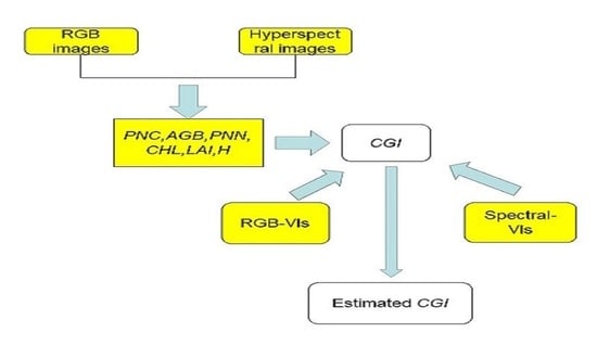
Specifically (see Figure 2), we calculated the vegetation indices from both the UAV RGB imagery and from the UAV hyperspectral images and analyzed them both by comparison with PNC, AGB, PWC, CHL, LAI, H, and CGI. The CGI estimation model was constructed using MLR, PLSR, and RF, and the maps of the CGI distribution based on the UAV-based RGB and spectral vegetation indices were generated.

2.6. Analysis Methods

We analyzed the correlation between the vegetation index and CGI and used multiple MLR, PLSR, and RF methods to build an estimation model. To estimate the CGI from a single vegetation index, to deal with multiple variables, we used MLR, PLSR, and RF. MLR can be used to accurately measure the degree of correlation between various factors and the degree of regression fitting to improve the prediction equation. The larger the absolute value of the standardized regression coefficient, the greater the effect of the corresponding independent variable on the dependent variable.

$$y=a_0+a_1{x}_{1n}+\cdots +a_m{x}_{mn}+w_m$$

(1)

In Equation (1), n is the number of modeling factors and a (= 1, …, m) is the coefficient.

PLSR can effectively eliminate collinearity among multiple variables, reduce multiple variables to fewer unrelated latent variables, maximize covariance between independent and dependent variables, and then establish regression models [29,30]. RF is based on the bootstrap sampling method whereby multiple samples are extracted from the original sample. The number of random forest algorithm trees we use is set to 1000, and the number of nodes is 50. Each bootstrap sample is modeled using a decision tree, and multiple decision trees are then combined for prediction. Finally, the prediction is determined by voting [31,32].

We used WiMATLAB2018a software (Matrix Laboratory 2014a, MathWorks, Inc., Natick, MA, USA) to calibrate and verify the model with the vegetation index as the input variable and the CGI as the output variable.

2.7. Selection of RGB Imagery Indices and Hyperspectral Indices

The vegetation index combines two or more pieces of spectral information, which can simply the measurement of vegetation states. The vegetation index is widely used for monitoring grassland, forest, and drought. To build a model to estimate the CGI, 13 RGB-imagery-based vegetation indices and 13 hyperspectral-image-based vegetation indices were selected (

Table 1. Indices from RGB imagery and from hyperspectral images.

Type	Index	Formula	References
RGB-imagery-based vegetation indices	R	R = R	[15]
	G	G = G	[15]
	B	B = B	[15]
	r	r = R/(R + G + B)	[15]
	g	g = G/(R + G + B)	[15]
	b	b = B/(R + G + B)	[15]
	EXR	EXR = 1.4 r − g	[33]
	VARI	VARI = (g − r)/(g + r − b)	[34]
	GRVI	GRVI = (g − r)/(g + r)	[35]
	MGRVI	MGRVI = (g2 − r2)/(g2 + r2)	[35]
	CIVE	CIVE = 0.441 r − 0.881 g + 0.385 b + 18.78745	[36]
	EXG	EXG = 2 g − b − r	[37]
	GLA	GLA = (2G – B − R)/(2G + B + R)	[38]
Hyperspectral-imagery-based vegetation indices	NDVI	(R800 − R680)/(R800 + R680)	[39]
	SR	R750/R550	[40]
	MSR	(R800/R760 − 1)/(R800/R670 + 1)1/2	[41]
	MCARI	((R700 − R670) − 0.2 × (R700 − R550))(R700/R670)	[42]
	TCARI	3[(R700 − R670) − 0.2(R700 − R550)(R700/R670)]	[42]
	MSAVI	0.5[2R800 + 1 − ((2R800 + 1)2 − 8(R800 − R670))1/2]	[43]
	OSAVI	1.16 × (R800 − R670)/(R800 + R670 + 0.16)	[8]
	EVI2	2.5 × (R800 − R670)/(R800 + 2.4 × R670 + 1)	[9]
	SPVI	0.4[3.7(R800 − R670) − 1.2|R530 − R670|]	[44]
	LCI	(R850 − R710)/(R850 + R680)	[45]
	RDVI	(R800 − R670)/(R800 + R670)1/2	[46]
	BGI	R460/R560	[47]
	NPCI	(R670 − R460)/(R670 + R460)	[48]

Note: R: red reflectance; G: green reflectance; B: blue reflectance; r: normalized red reflectance; g: normalized green reflectance; b: normalized blue reflectance; EXR: excess-red index; VARI: vegetation atmospherically resistant index; GRVI: green-red vegetation index; MGRVI: modified green-red vegetation index; CIVE: color index of vegetation; EXG: excess-green index; GLA: green leaf algorithm index; NDVI: normalized difference vegetation index; SR: simple ratio vegetation index; MSR: modified simple ratio index; MCARI: modified chlorophyll absorption ratio index; TCARI: transformed chlorophyll absorption ratio index; MSAVI: modified soil-adjusted vegetation index; OSAVI: optimized soil-adjusted vegetation index; EVI2: two-band enhanced VI; SPVI: spectral polygon vegetation index; LCI: linear combination index; RDVI: renormalized difference vegetation index; BGI: bare ground index; NPCI: normalized pigment chlorophyll ratio index.

).

2.8. Construction of Comprehensive Growth Index

In this study, we combine PNC, AGB, PWC, CHL, LAI, and H into a CGI. We take into account the different winter wheat growth stages when monitoring single growth phases versus the entire growth phase. In order to combine multiple agronomic parameters into a new index and provide guidance for future remote sensing yield monitoring, the PNC, AGB, PWC, CHL, LAI, and H are combined into CGI, which can not only reflect the growth information of crops but can also be correlated with yield. It is also of great significance to the monitoring of crops. Each parameter that constructs the CGI contributes to the construction of the model, so it is calculated in a weighted manner. For the time being, the contribution of each factor is the same; that is, the contribution of each factor to the construction of the model is the same. The PNC, AGB, PWC, CHL, LAI, and H are normalized separately:

$$W_t=X_t/max(X_t)$$

(2)

After normalizing PNC, AGB, PWC, CHL, LAI, and H, they are weighted by one-sixth and summed to form the CGI [15]:

$$CGI=\frac{1}{6} {{\displaystyle \sum }}_{t=1}^{6 } W_t$$

(3)

$$CGI=a\times W_{PNC}+b\times W_{AGB}+c\times W_{PWC}+d\times W_{CHL}+e\times W_{LAI}+f\times W_H$$

(4)

where t = PNC, AGB, PWC, CHL, LAI, and H; $X_t$ is the value of PNC, AGB, PWC, CHL, LAI, and H at each the growth stage; $max\left(X_t\right)$ is the maximum of PNC, AGB, PWC, CHL, LAI, and H at each the growth stage; $W_{t }$ is the normalized value; and a, b, c, d, e, f are each one-sixth.

2.9. Verification of Accuracy

We took the 48 data from each of the three winter wheat growth stages, used two sets of data as calibration sets (plant field 1, plant field 2; see Figure 1), and used the remaining set (plant field 3, Figure 1) as the validation set for constructing the model. The correlation coefficient was used to evaluate how the vegetation indices were related to the CGI. To evaluate the performance of the proposed model, we use the coefficient of determination R², the root-mean-squared error (RMSE), and the normalized root-mean-squared error (NRMSE). As a model evaluation standard [15], statistically speaking, higher R² values and lower RMSE and NRMSE correspond to a more accurate model. R², RMSE, and NRMSE are calculated as follows:

$$R^2=\frac{{{\displaystyle \sum }}_{i=1}^n{\left(x_i-\overline{x}\right)}^2{\left(y_i-\overline{y}\right)}^2}{{{\displaystyle \sum }}_{i=1}^n{\left(x_i-\overline{x}\right)}^2{{\displaystyle \sum }}_{i=1}^n{\left(y_i-\overline{y}\right)}^2}$$

(5)

$$RMSE=\sqrt{\frac{{{\displaystyle \sum }}_{i=1}^n{\left(x_i-y_i\right)}^2}{n}}$$

(6)

$$NRMSE=\frac{RMSE}{\overline{X}}\times 100\%$$

(7)

where $x_i$ is the measured CGI for winter wheat, $\overline{x}$ is the average measured CGI, $y_{i }$ is the predicted CGI, $\overline{y}$ is the average predicted CGI, and n is the number of model samples.

3. Results and Analysis

3.1. Correlation Analysis

To construct the proposed CGI and vegetation index, the RGB imagery indices and spectral indices of (GS 31), (GS 47), (GS 65) and for all three stages were combined with PNC, AGB, PWC, CHL, LAI, and H.

Table 2. Results of correlation analysis between RGB imagery indices and single indicator and the CGI.

Stages	Index	Correlation Coefficient
		PNC	AGB	PWC	CHL	LAI	H	CGI
(GS 31)	R	−0.56 **	−0.72 **	−0.66 **	−0.65 **	−0.78 **	−0.50 **	−0.85 **
	r	−0.72 **	−0.61 **	−0.69 **	−0.69 **	−0.65 **	−0.50 **	−0.81 **
	EXR	−0.64 **	−0.63 **	−0.63 **	−0.65 **	−0.69 **	−0.51 **	−0.81 **
	G	−0.47 **	−0.72 **	−0.64 **	−0.59 **	−0.78 **	−0.46 **	−0.80 **
	VARI	0.63 **	0.63 **	0.62 **	0.64 **	0.69 **	0.52 **	0.80 **
	MGRVI	0.63 **	0.63 **	0.61 **	0.64 **	0.69 **	0.52 **	0.80 **
	GRVI	0.63 **	0.63 **	0.61 **	0.64 **	0.69 **	0.52 **	0.80 **
	B	−0.35 *	−0.69 **	−0.52 **	−0.50 **	−0.76 **	−0.45 **	−0.73 **
	CIVE	−0.47 **	−0.61 **	−0.49 **	−0.52 **	−0.69 **	−0.49 **	−0.72 **
	GLA	0.45 **	0.60 **	0.48 **	0.51 **	0.68 **	0.49 **	0.71 **
	EXG	0.45 **	0.60 **	0.48 **	0.51 **	0.68 **	0.49 **	0.71 **
	g	0.45 **	0.60 **	0.48 **	0.51 **	0.68 **	0.49 **	0.71 **
	b	0.66 **	0.23	0.54 **	0.51 **	0.18	0.19	0.43 **
(GS 47)	R	−0.51 **	−0.68 **	−0.66 **	−0.45 **	−0.63 **	−0.48 **	−0.69 **
	r	−0.64 **	−0.73 **	−0.68 **	−0.53 **	−0.74 **	−0.70 **	−0.81 **
	EXR	−0.56 **	−0.71 **	−0.69 **	−0.43 **	−0.72 **	−0.72 **	−0.77 **
	G	−0.41 **	−0.57 **	−0.56 **	−0.41 **	−0.49 **	−0.23	−0.55 **
	VARI	0.55 **	0.70 **	0.69 **	0.42 **	0.72 **	0.72 **	0.76 **
	MGRVI	0.53 **	0.70 **	0.69 **	0.40 **	0.71 **	0.73 **	0.75 **
	GRVI	0.53 **	0.70 **	0.69 **	0.40 **	0.71 **	0.73 **	0.75 **
	B	−0.13	−0.40 **	−0.47 **	−0.11	−0.32	−0.13	−0.31 *
	CIVE	−0.24	−0.53 **	−0.62 **	−0.08	−0.56 **	−0.68 **	−0.52 **
	GLA	0.20	0.50 **	0.60 **	0.03	0.53 **	0.66 **	0.48 **
	EXG	0.20	0.50 **	0.60 **	0.03	0.53 **	0.66 **	0.48 **
	g	0.20	0.50 **	0.60 **	0.03	0.53 **	0.66 **	0.48 **
	b	0.76 **	0.70 **	0.56 **	0.72 **	0.69 **	0.56 **	0.83 **
(GS 65)	R	−0.40 **	−0.63 **	−0.67 **	−0.41 **	−0.63 **	−0.48 **	−0.79 **
	r	−0.49 **	−0.71 **	−0.79 **	−0.45 **	−0.74 **	−0.72 **	−0.81 **
	EXR	−0.37 **	−0.69 **	−0.72 **	−0.35 *	−0.68 **	−0.71 **	−0.79 **
	G	−0.39 **	−0.51 **	−0.55 **	−0.42 **	−0.51 **	−0.20	−0.67 **
	VARI	0.37 **	0.69 **	0.72 **	0.35 *	0.69 **	0.71 **	0.80 **
	MGRVI	0.35 *	0.68 **	0.71 **	0.33 *	0.67 **	0.70 **	0.79 **
	GRVI	0.35 *	0.68 **	0.71 **	0.33 *	0.67 **	0.70 **	0.79 **
	B	−0.14	−0.43 **	−0.39 **	−0.20	−0.39 **	−0.22	−0.59 **
	CIVE	−0.13	−0.59 **	−0.54 **	−0.16	−0.54 **	−0.63 **	−0.69 **
	GLA	0.11	0.57 **	0.52 **	0.15	0.52 **	0.62 **	0.68 **
	EXG	0.11	0.57 **	0.52 **	0.15	0.52 **	0.62 **	0.68 **
	g	0.11	0.57 **	0.52 **	0.15	0.52 **	0.62 **	0.68 **
	b	0.78 **	0.52 **	0.75 **	0.64 **	0.64 **	0.46 **	0.56 **
Total for three stages	R	−0.47 **	−0.64 **	−0.63 **	−0.48 **	−0.51 **	−0.50 **	−0.68 **
	r	−0.64 **	−0.65 **	−0.27 **	−0.45 **	−0.46 **	−0.68 **	−0.71 **
	EXR	−0.55 **	−0.67 **	−0.42 **	−0.44 **	−0.57 **	−0.67 **	−0.74 **
	G	−0.36 **	−0.53 **	−0.65 **	−0.42 **	−0.40 **	−0.32 **	−0.55 **
	VARI	0.54 **	0.68 **	0.42 **	0.43 **	0.57 **	0.68 **	0.74 **
	MGRVI	0.53 **	0.67 **	0.44 **	0.43 **	0.58 **	0.66 **	0.73 **
	GRVI	0.53 **	0.67 **	0.44 **	0.43 **	0.58 **	0.66 **	0.73 **
	B	−0.07	−0.36 **	−0.69 **	−0.24 **	−0.36 *	−0.15	−0.36 **
	CIVE	−0.19 *	−0.50 **	−0.59 **	−0.28 **	−0.57 **	−0.44 **	−0.55 **
	GLA	0.5	0.47 **	0.59 **	0.25 **	0.55 **	0.41 **	0.52 **
	EXG	0.15	0.47 **	0.59 **	0.25 **	0.56 **	0.41 **	0.52 **
	g	0.15	0.47 **	0.59 **	0.25 **	0.56 **	0.41 **	0.52 **
	b	0.61 **	0.41 **	−0.11	0.33 **	0.15	0.48 **	0.44 **

Note: * indicates a significant correlation at 0.05 level; ** indicates a significant correlation at 0.1 level.

and

Table 3. Results of correlation analysis between the spectral indices, single indicator, and the CGI.

Stages	Index	Correlation Coefficient
		PNC	AGB	PWC	CHL	LAI	H	CGI
(GS 31)	LCI	0.62 **	0.67 **	0.65 **	0.75 **	0.70 **	0.48 **	0.83 **
	MSR	0.63 **	0.64 **	0.63 **	0.69 **	0.66 **	0.48 **	0.80 **
	SR	0.64 **	0.63 **	0.65 **	0.67 **	0.65 **	0.49 **	0.79 **
	NDVI	0.57 **	0.62 **	0.57 **	0.70 **	0.65 **	0.45 **	0.77 **
	NPCI	−0.68 **	−0.58 **	−0.63 **	−0.67 **	−0.62 **	−0.42 **	−0.77 **
	OSAVI	0.52 **	0.44 **	0.42 **	0.66 **	0.49 **	0.32 *	0.62 **
	BGI	0.57 **	0.45 **	0.70 **	0.49 **	0.45 **	0.26	0.58 **
	RDVI	0.49 **	0.37 **	0.35 *	0.61 **	0.42 **	0.27	0.54 **
	EVI2	0.45 **	0.30 *	0.30 *	0.56 **	0.35 *	0.22	0.47 **
	MSAVI	0.45 **	0.29 *	0.30 *	0.56 **	0.35 *	0.23	0.47 **
	SPVI	0.38 **	0.20	0.21	0.49 **	0.25	0.15	0.36 **
	TCARI	−0.12	−0.31 *	−0.42 **	−0.09	−0.28	−0.27	−0.29 *
	MCARI	0.19	0.01	−0.07	0.22	0.06	0.02	0.11
(GS 47)	LCI	0.68 **	0.78 **	0.64 **	0.60 **	0.74 **	0.69 **	0.85 **
	MSR	0.63 **	0.76 **	0.62 **	0.51 **	0.73 **	0.73 **	0.82 **
	NDVI	0.63 **	0.76 **	0.58 **	0.53 **	0.70 **	0.74 **	0.81 **
	SR	0.62 **	0.75 **	0.63 **	0.49 **	0.73 **	0.72 **	0.81 **
	OSAVI	0.67 **	0.74 **	0.46 **	0.51 **	0.68 **	0.79 **	0.81 **
	NPCI	−0.61 **	−0.75 **	−0.65 **	−0.49 **	−0.71 **	−0.71 **	−0.80 **
	RDVI	0.68 **	0.70 **	0.39 **	0.49 **	0.66 **	0.80 **	0.78 **
	MSAVI	0.67 **	0.70 **	0.38 **	0.48 **	0.65 **	0.80 **	0.78 **
	EVI2	0.67 **	0.69 **	0.36 *	0.47 **	0.64 **	0.80 **	0.77 **
	SPVI	0.66 **	0.63 **	0.28	0.44 **	0.60 **	0.79 **	0.72 **
	BGI	0.58 **	0.65 **	0.67 **	0.54 **	0.61 **	0.44 **	0.71 **
	TCARI	−0.24	−0.37 **	−0.61 **	−0.38 **	−0.37 **	0.01	−0.38 **
	MCARI	0.06	0.05	−0.26	−0.16	0.01	0.45 **	0.05
(GS 65)	LCI	0.55 **	0.77 **	0.79 **	0.53 **	0.78 **	0.66 **	0.84 **
	MSAVI	0.48 **	0.80 **	0.75 **	0.41 **	0.77 **	0.79 **	0.83 **
	SPVI	0.48 **	0.80 **	0.74 **	0.41 **	0.77 **	0.80 **	0.83 **
	EVI2	0.48 **	0.79 **	0.75 **	0.42 **	0.77 **	0.79 **	0.82 **
	RDVI	0.48 **	0.78 **	0.76 **	0.43 **	0.76 **	0.79 **	0.82 **
	SR	0.45 **	0.81 **	0.78 **	0.40 **	0.80 **	0.69 **	0.82 **
	MSR	0.46 **	0.80 **	0.79 **	0.42 **	0.78 **	0.71 **	0.82 **
	OSAVI	0.48 **	0.77 **	0.77 **	0.44 **	0.76 **	0.77 **	0.82 **
	NDVI	0.45 **	0.73 **	0.76 **	0.44 **	0.72 **	0.71 **	0.77 **
	BGI	0.61 **	0.71 **	0.62 **	0.61 **	0.69 **	0.42 **	0.77 **
	NPCI	−0.40 **	−0.75 **	−0.76 **	−0.38 **	−0.72 **	−0.74 **	−0.76 **
	MCARI	−0.05	0.49 **	0.45 **	−0.03	0.40 **	0.81 **	0.40 **
	TCARI	−0.20	0.20	0.19	−0.20	0.12	0.72 **	0.14
Total for three stages	LCI	0.63 **	0.74 **	0.40 **	0.60 **	0.65 **	0.60 **	0.82 **
	MSR	0.58 **	0.74 **	0.52 **	0.52 **	0.63 **	0.65 **	0.80 **
	SR	0.58 **	0.74 **	0.52 **	0.50 **	0.63 **	0.64 **	0.80 **
	NDVI	0.55 **	0.69 **	0.50 **	0.54 **	0.59 **	0.62 **	0.76 **
	OSAVI	0.54 **	0.63 **	0.54 **	0.49 **	0.48 **	0.62 **	0.70 **
	NPCI	−0.55 **	−0.65 **	−0.51 **	−0.41 **	−0.40 **	−0.67 **	−0.67 **
	RDVI	0.52 **	0.58 **	0.54 **	0.46 **	0.42 **	0.61 **	0.65 **
	MSAVI	0.50 **	0.56 **	0.53 **	0.43 **	0.39 **	0.59 **	0.62 **
	EVI2	0.50 **	0.55 **	0.53 **	0.43 **	0.38 **	0.59 **	0.62 **
	SPVI	0.46 **	0.49 **	0.51 **	0.38 **	0.32 **	0.55 **	0.55 **
	BGI	0.50 **	0.49 **	0.43 **	0.33 **	0.15	0.47 **	0.48 **
	TCARI	−0.11	−0.13	0.23 **	−0.16	−0.28 **	0.13	−0.16
	MCARI	0.07	0.13	0.39 **	0.01	−0.05	0.34 **	0.12

Note: * indicates a significant correlation at 0.05 level; ** indicates a significant correlation at 0.1 level.

list the correlation between CGI, RGB imagery indices, and spectral indices. These results show that the correlation between the RGB imagery indices and PNC, AGB, PWC, CHL, LAI, and H depends on the growth period, and most of these correlations are very significant (significance level of 0.01).

We find that the RGB imagery indices r, EXR, VARI, and MGRVI correlate with the CGI during different growth stages, and the correlation coefficients are all higher than those between (i) r, EXR, VARI, MGRVI and (ii) PNC, AGB, PWC, CHL, LAI, and H. Thus, the correlation coefficients between RGB imagery indices r, EXR, VARI, MGRVI, and the CGI for the four growth stages are greater than the correlation coefficients between the individual crop-growth indicators. For the spectral indices, the correlation between the hyperspectral CGI and PNC, AGB, PWC, CHL, LAI, and H also hovers around 0.01. From (GS 31) to the total for the three stages, the correlation between the spectral index and the six crop-growth indicators varies irregularly. However, the spectral indices LCI, MSR, SR, and NDVI are more strongly correlated with the CGI than with the six crop-growth indicators. Thus, the CGI provides more accurate estimates of the crop-growth parameters.

3.2. Estimate of CGI Based on RGB Imagery and Spectral Indices

According to the results given in Table 2 and Table 3, we select the RGB-imagery indices r, EXR, VARI, and MGRVI and the spectral indices LCI, MSR, SR, and NDVI to estimate CGI.

The RGB-imagery indices r, EXR, VARI, and MGRVI and the spectral indices LCI, MSR, SR, and NDVI are taken as factors in (GS 31), (GS 47), (GS 65) and for all three stages, respectively. We then construct the CGI models based on the RGB-imagery indices r, EXR, VARI, and MGRVI and on the spectral indices LCI, MSR, SR, and NDVI for the different growth stages (see

Table 4. CGI estimation model for the single index of winter wheat in different stages.

Growth Stages	Parameters	Equations	Calibration			Verification
			R2	RMSE	NRMSE (%)	R2	RMSE	NRMSE (%)
(GS 31)	r	y = 8.7269 × e−6.874x	0.67	0.05	6.55	0.78	0.04	4.98
	EXR	y = 1.0729 × e−3.196x	0.65	0.05	6.73	0.73	0.04	5.49
	VARI	y = 0.6664 × e1.8637x	0.64	0.05	6.78	0.72	0.04	5.58
	MGRVI	y = 0.6655 × e1.449x	0.64	0.05	6.79	0.71	0.04	5.66
	LCI	y = 0.3945 × e1.067x	0.72	0.04	5.92	0.74	0.04	5.38
	MSR	y = 0.5264 × e0.1375x	0.67	0.05	6.48	0.69	0.05	5.93
	SR	y = 0.5844 × e0.0259x	0.66	0.05	6.65	0.68	0.05	6.03
	NDVI	y = 0.3222 × e1.0736x	0.63	0.05	6.84	0.65	0.05	6.25
(GS 47)	r	y = −5.5464x + 2.6602	0.57	0.06	8.14	0.84	0.04	5.09
	EXR	y = −2.9535x + 1.0445	0.50	0.07	8.71	0.75	0.05	6.32
	VARI	y = 1.5784x + 0.615	0.50	0.07	8.74	0.75	0.05	6.36
	MGRVI	y = 1.3382x + 0.6099	0.49	0.07	8.84	0.73	0.05	6.61
	LCI	y = 0.2967 × e1.4913x	0.69	0.05	7.04	0.84	0.04	5.50
	MSR	y = 0.1306x + 0.3858	0.62	0.06	7.67	0.81	0.04	5.63
	SR	y = 0.0223x + 0.5101	0.60	0.06	7.80	0.80	0.04	5.73
	NDVI	y = 0.1654 × e1.8498x	0.62	0.06	7.71	0.80	0.04	5.80
(GS 65)	r	y = −5.74x + 2.7027	0.55	0.06	7.80	0.70	0.05	7.33
	EXR	y = −2.5008x + 0.9961	0.45	0.07	8.65	0.59	0.06	8.56
	VARI	y = 1.3211x + 0.6346	0.46	0.07	8.62	0.59	0.06	8.50
	MGRVI	y = 1.0881x + 0.6362	0.43	0.07	8.78	0.57	0.06	8.76
	LCI	y = 0.32 × e1.3239x	0.67	0.05	6.74	0.75	0.05	6.46
	MSR	y = 01141x + 0.4495	0.62	0.06	7.24	0.72	0.05	7.02
	SR	y = 0.0209x + 0.5405	0.62	0.06	7.19	0.75	0.05	6.65
	NDVI	y = 0.2602 × e1.3278x	0.58	0.06	7.50	0.64	0.06	7.83
Total for three stages	r	y = 4.138x + 2.1912	0.54	0.06	8.04	0.62	0.06	7.67
	EXR	y = −2.4047x + 1.0012	0.57	0.06	7.75	0.52	0.07	8.69
	VARI	y = 1.3196x + 0.6485	0.57	0.06	7.79	0.52	0.07	8.65
	MGRVI	y = 1.0988x + 0.6455	0.57	0.06	7.78	0.50	0.07	8.86
	LCI	y = 0.893x + 0.2007	0.69	0.05	6.64	0.70	0.05	6.84
	MSR	y = 0.4986 × e0.1513x	0.63	0.06	7.25	0.66	0.06	7.19
	SR	y = 0.0203x + 0.5462	0.62	0.06	7.31	0.67	0.05	7.17
	NDVI	y = 0.265 × e1.3008x	0.59	0.06	7.57	0.61	0.06	7.72

).

The CGI model based on the RGB imagery indices r, EXR, VARI, and MGRVI generally performs well for all three growth stages and for the total of the three stages. The best performance for the RGB imagery index model is for the (GS 31). Overall, R² is higher and the RMSE and NMRSE are lower. At the same time, several pairs of RGB imagery–index calibration sets have the same R² and RMSE, such as VARI and MGRVI. The effect of the model becomes apparent only upon comparing NRMSE. The smaller the NRMSE, the higher the prediction accuracy. Of course, we also need to consider R², RMSE, and NRMSE for the validation set. Similarly, the effects of EXR, VARI, and the two RGB imagery indices used to construct the CGI model during (GS 47) need to be analyzed by NRMSE. The CGI effect of each growth stage is compared. The best-performing RGB indices are r, r, r, and EXR.

In the estimation model based on the spectral indices LCI, MSR, SR, and NDVI, evaluating models based on different spectral indices also requires comparing the magnitudes of R², RMSE, and NRMSE. We find that the difference between the R² of different estimation models is relatively clear. Combining these spectral indices with the results of the validation model allows us to evaluate the performance of different spectral index models. A comparison of the results of each model shows that the estimation model based on LCI gives the most accurate results.

3.3. Using RGB VIs and Spectral VIs with Machine Learning to Estimate CGI

Table 5. Results of using different methods to estimate the CGI for different winter wheat growth stages.

Growth Stages	Methods	Data	R2	RMSE	NRMSE (%)
(GS 31)	MLR	RGB, VIs	0.73	0.04	5.69
		Spectral, VIs	0.77	0.04	5.29
	PLSR	RGB, VIs	0.65	0.05	6.54
		Spectral VIs	0.66	0.05	6.40
	RF	RGB, VIs	0.53	0.06	7.64
		Spectral, VIs	0.64	0.05	6.66
(GS 47)	MLR	RGB, VIs	0.65	0.06	7.37
		Spectral, VIs	0.72	0.05	6.57
	PLSR	RGB, VIs	0.50	0.07	8.73
		Spectral, VIs	0.60	0.06	7.80
	RF	RGB, VIs	0.42	0.08	9.65
		Spectral, VIs	0.50	0.07	8.76
(GS 65)	MLR	RGB, VIs	0.68	0.05	6.63
		Spectral, VIs	0.78	0.04	5.44
	PLSR	RGB, VIs	0.62	0.05	6.93
		Spectral, VIs	0.65	0.05	5.88
	RF	RGB, VIs	0.54	0.06	7.97
		Spectral, VIs	0.60	0.06	7.38
Total for three stages	MLR	RGB, VIs	0.58	0.06	7.71
		Spectral, VIs	0.69	0.05	6.61
	PLSR	RGB, VIs	0.57	0.06	7.77
		Spectral, VIs	0.62	0.06	7.30
	RF	RGB, VIs	0.48	0.07	8.62
		Spectral, VIs	0.57	0.06	7.81

shows the modeling analysis based on the four RGB imagery indices, the four spectral indices, and the CGI estimated by using MLR, PLSR, and RF.

Comparing the estimation of the CGI result based on indices built from RGB imagery with that based on the spectral indices from the different growth stages, we find that the latter is superior to the former. In addition, a comparison with different machine learning methods shows that the CGI estimation model constructed using MLR is the most accurate of the three methods, followed by the model constructed from PLSR, and finally by the model constructed from RF, which shows that MLR method is the index, followed by PLSR, and finally by RF. We now use the verification set data to verify the RGB-imagery -based index and spectral-based index combined with the MLR, PLSR, and RF methods to estimate the CGI. Figure 3 and Figure 4 show the relationship between the measured and predicted values (y = ax + b, R², RMSE, NRMSE). The results show that the verification is consistent with the modeling, and the fit is very good (the fit to the spectral index is better than the fit to the RGB-imagery index). Comprehensive modeling and verification (see Table 5 and Figure 3 and Figure 4) show that the MLR, PLSR, and RF methods all provide a more accurate estimate of the CGI than the single RGB-imagery index or the single spectral index (see Table 4 and Table 5 and Figure 3 and Figure 4). Thus, these three methods all provide good estimates of the CGI.

3.4. Map of CGI Distribution

Estimating the CGI by using machine learning and based on RGB-imagery-based indices and spectral-based indices allows us to select the best estimation model for the different growth stages. Figure 5 and Figure 6 show the results of applying the MLR estimation model to the UAV RGB and hyperspectral imagery of (GS 31), (GS 47), and (GS 65).

From jointing to flowering, the average RGB-based CGI ranges from 0.74 to 0.79 (Figure 5) and hyperspectral-based CGI averages from 0.74 to 0.78 (Figure 6). In addition, the corresponding CGI map is greener, indicating a higher CGI. The current map also shows that the CGI has increased during the three growing seasons of winter wheat. These results are consistent with the actual observations. The CGI distribution based on the RGB and hyperspectral UAV images shows the difference between CGI estimation models based on the two types of data (Figure 7). The predicted CGI values differ, which leads to different CGI distributions for the same growth stage. However, the results for the three growth stages show that winter wheat growth is best in plant field 2 and is relatively stable over the different growth stages. The map of the CGI distribution clearly differentiates between the better-growing areas and the poorer-growing areas.

4. Discussion

4.1. Single Growth-Monitoring Indicators and CGI for Winter Wheat

From (GS 31) to the total for the three stages, most of the RGB imagery indices and hyperspectral indices are significantly correlated with PNC, AGB, PWC, CHL, LAI, H, and CGI (Table 2 and Table 3). The RGB imagery indices R, EXR, VARI, MGRVI, and CGI are more strongly correlated than r, EXR, VARI, MGRVI and PNC, AGB, PWC, CHL, LAI, and H, which shows that the four RGB imagery indices for the CGI are very sensitive. Zhou et al. [49] used EXR and VARI to monitor rice growth and obtained more accurate predictions. Niu et al. [50] used UAV RGB imagery to show that r and MGRVI can provide good estimates of the LAI.

Over the four growth stages, the hyperspectral indices LCI, MSR, SR, and NDVI are more strongly correlated with the CGI than LCI, MSR, SR, and NDVI are with PNC, AGB, PWC, CHL, LAI, and H. These four spectral indices are more sensitive to the CGI, mainly because the CGI contains more information about crop growth. Yue et al. [15] found that the LCI is useful for monitoring the AGB and LAI of winter wheat. Wu et al. [42] explored the use of the MSR and NDVI to estimate CHL. Liang et al. [51] accurately estimated crop parameters by using the SR. These studies show that these spectral indices are reliable for monitoring crop parameters. At present, the monitoring of crop growth focuses on single indices, which monitor crop growth based on a single growth parameter. Zhu et al. [52] used several spectral LNC indices to confirm their effectiveness for quantitatively inversing the LNC of winter wheat. However, the sensitivities of the RGB imagery, spectral index, and various growth parameters differ. Some RGB imagery and spectral indices may be highly sensitive to one growth parameter and less sensitive to another. The proposed CGI combines six growth-monitoring parameters and considers various combinations of growth parameters. Based on the correlation between the RGB-imagery and hyperspectral indices and the CGI, the CGI can be used as an index to monitor crop growth.

4.2. Estimation of CGI Based on a Single Index

The RGB imagery indices r, EXR, VARI, and MGRVI and the spectral indices LCI, MSR, SR, and NDVI, which are strongly correlated with the CGI, are used to construct the CGI estimation model. The results show that the models constructed for single growth stages and multiple growth stages both provide good estimates (Table 4). Moreover, the findings indicate that the CGI can be accurately estimated from a single RGB imagery index or from a single hyperspectral index. The optimal CGI models of the RGB imagery index at (GS 31), (GS 47), (GS 65), and all three stages have different indices that reflect the various sensitivities of the RGB imagery indices in different growth stages. In addition, the indices provide CGI predictions of varying accuracy. The performance of the spectral parameters and RGB imagery indices varies over the four stages. In conclusion, the LCI provides the best spectral index for estimating the CGI over the different growth stages, and the models constructed for the four growth stages are the most satisfactory. Therefore, the optimal estimation of the CGI based on the spectral index is more stable than that based on an RGB imagery index.

Some RGB imagery and spectral indices saturate the growth parameters. Thus, we should further investigate how to estimate the growth parameters [53]. The PNC, AGB, PWC, CHL, LAI, and H from the (GS 31) to the (GS 65) of winter wheat all change to varying degrees, and these changes modify the CGI in the different growth stages. At (GS 31) and (GS 47), the photosynthates are mainly stored in stems and leaves, whereas, at the flowering stage, they are stored in flowers and in the wheat ear. Thus, using a visible-light vegetation index is not recommended for estimating AGB [15]. Although the RGB-image and hyperspectral indices at various growth stages are related to six growth parameters, the vegetation index monitoring crop growth effect is related to dry matter and pigment [6], which means that the sensitivity of an index to the CGI also depends on the winter wheat’s growth stage. For instance, the LCI is highly sensitive to the four growth stages of winter wheat. Therefore, the optimal predictive factor for estimating CGI should be determined.

4.3. Estimation of CGI Based on Multiple Indices Combined with Machine Learning

Machine learning methods are increasingly used to estimate parameters to monitor crop growth. The results of this study show that machine-learning estimates of growth parameters based on multiple RGB imagery or spectral indices are more accurate than single-index estimates. Yue et al. [54] used the PLSR to obtain better estimates of the AGB than is possible by using a single vegetation index. Han et al. [20] used multiple linear regression, partial least squares regression, artificial neural networks, and the random forest algorithm to improve the accuracy of estimates of AGB. Better estimates of crop parameters can be obtained by using machine learning methods, which is consistent with the research results presented herein. The CGI estimation model constructed by MLR is better than a model based on a single RGB imagery index or a single spectral index. Estimates made using the PLSR or RF models are also better than most (but not all) single RGB imagery index or spectral index models (see Table 4 and Table 5 and Figure 3 and Figure 4), which may be related to the number of variables involved in the construction of these models. According to Yue et al. [15], given sufficient input variables, the models constructed by PLSR and RF provide better estimation.

The MLR model based on RGB imagery and spectral indices is superior to the PLSR and RF models over the different growth stages (see Table 5 and Figure 3 and Figure 4), which we attribute to one of the three following reasons: (i) An index that is strongly correlated with the CGI is preferable for the construction of the model. (ii) A model made from a linear estimate by a single index provides good results. The sensitivity of multiple indices is combined with the CGI, resulting in an abundant amount of information. (iii) RF is suitable for processing large amounts of data but is disadvantaged for processing small data sets. Han et al. [20] and Ozlem et al. [55] used large sample data and the RF algorithm to improve the prediction the model.

In addition, since this paper uses empirical models, although Zhou et al. [49], Niu et al. [50], Yue et al. [15], Wu et al. [42], and Liang et al. [51] used the vegetation index from the estimation model used herein, the crop parameters were estimated by using empirical methods. However, to estimate crop canopy variables, one must consider confounding factors that also affect the estimation, such as leaf or canopy structure and the understory in multiple-scattering processes, soil parameters, and some external parameters [56,57,58,59,60,61]. To determine how canopy structure affects estimates of crop parameters, Bendig et al. [62] used UAV RGB imagery to obtain crop surface models, extract crop heights, and use the extracted crop heights to estimate biomass, which improved the accuracy of the estimates. In the next step, we further study how to estimate crop parameters based on crop height to explore how various sensors affect estimates.

4.4. CGI Estimation Based on Different Sensors

The results of this study show that using a single index versus multiple indices combined with machine learning to estimate CGI produces different results. This research shows that an RGB camera mounted on a UAV can be used to accurately estimate crop-growth parameters, assess the data of cameras mounted on UAVs are reliable [63], but the accuracy of such estimates based on UAV hyperspectral data estimation is higher. Yue et al. [15] monitored crop LAI and AGB and found that the monitoring by using UAV hyperspectral cameras is better than by using UAV RGB cameras. The results are consistent with the performance of the two sensors and with the two estimated CGIs. The CGI model estimated by the UAV hyperspectral data is superior to that estimated by the UAV RGB imagery. Therefore, hyperspectral sensors are preferred for monitoring crop growth. The results of the RGB camera are close to the results of using a hyperspectral sensor, considering the cost issue, and the simpler data processing of RGB, it is recommended to use an RGB sensor on the UAV.

Note that this study still has several shortcomings. The research area is limited to Changping District, Beijing, China. The growth of winter wheat in other regions, as well as other varieties of wheat grown in different years, should be further investigated to verify the findings of this research. In addition, the CGI calculates the average weight of the growth indicators at different growth stages, so the weight of the growth index should be distributed on the basis of growth stages to improve the results. At present, we use UAV to carry RGB cameras and hyperspectral cameras for experiments. In the future, we can use multispectral or lidar sensors to conduct experiments to explore the impact of different sensors on the experimental results. At the same time, in the future, different weight ratios will be assigned to the contribution of different factors in the model construction to explore the estimation effect of the model under different ratios.

5. Conclusions

Six growth indicators were used to construct a new CGI index. The CGI of winter wheat at different growth stages was estimated by using UAV RGB imagery and hyperspectral data. The linear, nonlinear, MLR, PLSR, and RF models were further developed. The main conclusions are as follows: The RGB imagery indices r, EXR, VARI, and MGRVI are more strongly correlated with the CGI for the growth stages than are PNC, AGB, PWC, CHL, LAI, and H. The spectral indices LCI, MSR, SR, and NDVI are more strongly correlated with the CGI than the single growth-monitoring index for the four stages, which indicates that the CGI can be used to monitor crop growth. On the one hand, the CGI model from a single RGB imagery index has different optimal indices at different growth stages. On the other hand, the model constructed by using a single spectral index has the best index in each growth stage, all of which are in terms of the LCI. By combining multiple RGB imagery indices and spectral indices with MLR, PLSR, and RF to estimate the CGI, the MLR model is optimal for different growth stages, the PLSR model is second best, and the RF model is the worst. The best model based on RGB-imagery indices gives R², RMSE, and NRMSE of 0.73, 0.04, 5.69%, and the best model based on hyperspectral data gives an R², RMSE, and NRMSE of 0.78, 0.04, and 5.29%, respectively. The CGI can be accurately estimated by using UAV RGB imagery and hyperspectral data. Both methods can estimate the CGI. However, the hyperspectral data lead to more accurate estimates of the CGI than the RGB imagery, which demonstrates that UAV hyperspectral imaging provides more accurate results. Currently, developments are underway for UAV payloads, including hyperspectral, LIDAR, synthetic aperture radars, and thermal infrared sensors. Fully comparing the advantages of each sensor type requires further study.

References

1. Li, X.; Zhang, Y.; Luo, J.; Jin, X.; Xu, Y.; Yang, W. Quantification winter wheat LAI with HJ-1CCD image features over multiple growing seasons. Int. J. Appl. Earth Obs. Geoinf. 2016, 44, 104–112. [Google Scholar] [CrossRef]
2. Campos, M.; García, F.J.; Camps, G.; Grau, G.; Nutini, F.; Crema, A.; Boschetti, M. Multitemporal and multiresolution leaf area index retrieval for operational local rice crop monitoring. Remote Sens. Environ. 2016, 187, 102–118. [Google Scholar] [CrossRef]
3. Jin, X.; Kumar, L.; Li, Z.; Xu, X.; Yang, G.; Wang, J. Estimation of winter wheat biomass and yield by combining the aquacrop model and field hyperspectral data. Remote Sens. 2016, 8, 972. [Google Scholar] [CrossRef] [Green Version]
4. Launay, M.; Guerif, M. Assimilating remote sensing data into a crop model to improve predictive performance for spatial applications. Agric. Ecosyst. Environ. 2005, 111, 321–339. [Google Scholar] [CrossRef]
5. Di Gennaro, S.F.; Toscano, P.; Gatti, M.; Poni, S.; Berton, A.; Matese, A. Spectral comparison of UAV-Based hyper and multispectral cameras for precision viticulture. Remote Sens. 2022, 14, 449. [Google Scholar] [CrossRef]
6. Berger, K.; Atzberger, C.; Danner, M.; D’Urso, G.; Mauser, W.; Vuolo, F.; Hank, T. Evaluation of the PROSAIL model capabilities for future hyperspectral model environments: A review study. Remote Sens. 2018, 10, 85. [Google Scholar] [CrossRef] [Green Version]
7. Taniguchi, K.; Obata, K.; Yoshioka, H. Derivation and approximation of soil isoline equations in the red–near-infrared reflflectance subspace. J. Appl. Remote Sens. 2014, 8, 083621. [Google Scholar] [CrossRef] [Green Version]
8. Wang, W.; Gao, X.; Cheng, Y.; Ren, Y.; Zhang, Z.; Wang, R.; Cao, J.; Geng, H. QTL mapping of leaf area index and chlorophyll content based on UAV remote sensing in wheat. EconPapers. 2022, 12, 595. [Google Scholar] [CrossRef]
9. Zhang, H.; Tang, Z.; Wang, B.; Meng, B.; Qin, Y.; Sun, Y.; Lv, Y.; Zhang, J.; Yi, S. A non-destructive method for rapid acquisition of grassland aboveground biomass for satellite ground verification using UAV RGB images. Glob. Ecol. Conserv. 2022, 33, e01999. [Google Scholar] [CrossRef]
10. Xu, L.; Zhou, L.; Meng, R.; Zhang, F.; Lv, Z.; Xu, B.; Zeng, L.; Yu, X.; Peng, S. An improved approach to estimate ratoon rice aboveground biomass by integrating UAV-based spectral, textural and structural features. Precis. Agric. 2022, 23, 1276–1301. [Google Scholar] [CrossRef]
11. Jin, X.; Liu, S.; Baret, F.; Hemerlé, M.; Comar, A. Estimates of plant density of wheat crops at emergence from very low altitude UAV imagery. Remote Sens. Environ. 2017, 198, 105–114. [Google Scholar] [CrossRef] [Green Version]
12. Yu, N.; Li, L.; Schmitz, N.; Tian, L.F.; Greenberg, J.A.; Diers, B.W. Development of methods to improve soybean yield estimation and predict plant maturity with an unmanned aerial vehicle based platform. Remote Sens. Environ. 2016, 187, 91–101. [Google Scholar] [CrossRef]
13. Maimaitijiang, M.; Ghulam, A.; Sidike, P.; Hartling, S.; Maimaitiyiming, M.; Peterson, K.; Shavers, E.; Fishman, J.; Peterson, J.; Kadam, S.; et al. Unmanned Aerial System (UAS)-based phenotyping of soybean using multi-sensor data fusion and extreme learning machine. ISPRS J. Photogramm. Remote Sens. 2017, 134, 43–58. [Google Scholar] [CrossRef]
14. Adar, S.; Sternberg, M.; Paz-Kagan, T.; Henkin, Z.; Dovrat, G.; Zaady, E. Argaman E. Estimation of aboveground biomass production using an unmanned aerial vehicle (UAV) and VENμS satellite imagery in Mediterranean and semiarid rangelands. Remote Sens. Appl. Soc. Environ. 2022, 26, 100753. [Google Scholar]
15. Yue, J.; Feng, H.; Jin, X.; Yuan, H.; Li, Z.; Zhou, C.; Yang, G.; Tian, Q. A Comparison of Crop Parameters Estimation Using Images from UAV-Mounted Snapshot Hyperspectral Sensor and High-Definition Digital Camera. Remote Sens. 2018, 10, 1138. [Google Scholar] [CrossRef] [Green Version]
16. Geipel, J.; Link, J.; Claupein, W. Combined spectral and spatial modeling of corn yield based on aerial images and crop surface models acquired with an unmanned aircraft system. Remote Sens. 2014, 6, 10335–10355. [Google Scholar] [CrossRef] [Green Version]
17. Zaman-Allah, M.; Vergara, O.; Araus, J.; Tarekegne, A.; Magorokosho, C.; Zarco-Tejada, P.; Hornero, A.; Albà, A.; Das, B.; Craufurd, P.; et al. Unmanned aerial platform-based multi-spectral imaging for field phenotyping of maize. Plant Methods 2015, 11, 35. [Google Scholar] [CrossRef] [Green Version]
18. Kefauver, S.C.; Vicente, R.; Vergara-Diaz, O.; Fernandez-Gallego, J.A.; Serret, M.M.D.; Araus, J.L.; Kerfal, S.; Lopez, A.; Melichar, J.P.E. Comparative UAV and field phenotyping to assess yield and nitrogen use efficiency in hybrid and conventional barley. Front. Plant Sci. 2017, 8, 1733. [Google Scholar] [CrossRef]
19. Chen, P.; Li, G.; Shi, Y.; Xu, Z.; Yang, F.; Cao, Q. Validation of an unmanned aerial vehicle hyperspectral sensor and its application in maize leaf area index estimation. Sci. Agric. Sin. 2018, 51, 1464–1474. [Google Scholar]
20. Han, L.; Yang, G.; Dai, H.; Xu, B.; Yang, H.; Feng, H.; Li, Z.; Yang, X. Modeling maize above-ground biomass based on machine learning approaches using UAV remote-sensing data. Plant Methods 2019, 15, 10. [Google Scholar] [CrossRef] [Green Version]
21. Swain, K.; Thomson, S.; Jayasuriya, H. Adoption of an Unmanned Helicopter for Low-Altitude Remote Sensing to Estimate Yield and Total Biomass of a Rice Crop. Trans. ASABE 2010, 53, 21–27. [Google Scholar] [CrossRef] [Green Version]
22. Chang, X.; Chang, Q.; Wang, X.; Chu, D.; Guo, R. Estimation of maize leaf chlorophyll contents based on UAV hyperspectral drone image. Agric. Res. Arid. Areas 2019, 37, 66–73. [Google Scholar]
23. Schirrmann, M.; Giebel, A.; Gleiniger, F.; Pflanz, M.; Lentschke, J.; Dammer, K.-H. Monitoring agronomic parameters of winter wheat crops with low-cost UAV imagery. Remote Sens. 2016, 8, 706. [Google Scholar] [CrossRef] [Green Version]
24. Li, Z.; Nie, C.; Wei, C.; Xu, X.; Song, X.; Wang, J. Comparison of four chemometric techniques for estimating leaf nitrogen concentrations in winter wheat (Triticum aestivum) based on hyperspectral features. J. Appl. Spectrosc. 2016, 83, 240–247. [Google Scholar] [CrossRef]
25. Duan, S.; Li, Z.; Wu, H.; Tang, B.; Ma, L.; Zhao, E.; Li, C. Inversion of the PROSAIL model to estimate leaf area index of maize, potato, and sunflower fields from unmanned aerial vehicle hyperspectral data. Int. J. Appl. Earth Obs. Geoinf. 2014, 26, 12–20. [Google Scholar] [CrossRef]
26. Li, J.; Zhu, X.; Ma, L.; Zhao, Y.; Qian, Y.; Tang, L. Leaf Area Index Retrieval and Scale Effect Analysis of Multiple Crops from UAV-based Hyperspectral Data. Remote Sens. Technol. Appl. 2017, 32, 427–434. [Google Scholar]
27. Lucieer, A.; Malenovsky, Z.; Veness, T.; Wallace, L. HyperUAS-imaging spectroscopy from a multirotor unmanned aircraft system. J. Field Robot. 2014, 31, 571–590. [Google Scholar] [CrossRef] [Green Version]
28. Turner, D.; Lucieer, A.; Wallace, L. Direct Georeferencing of Ultrahigh-Resolution UAV Imagery. IEEE Trans. Geosci. Remote Sens. 2014, 52, 2738–2745. [Google Scholar] [CrossRef]
29. Darvishzadeh, R.; Skidmore, A.; Schlerf, M.; Atzberger, C.; Corsi, F.; Cho, M. Lai and chlorophyll estimation for a heterogeneous grassland using hyperspectral measurements. ISPRS J. Photogramm. Remote Sens. 2008, 63, 409–426. [Google Scholar] [CrossRef]
30. Kuangnan, F.; Jianbin, W.; Jianping, Z.; Bangchang, X. A review of technologies on random forests. Stat. Inf. Forum 2011, 26, 32–38. [Google Scholar]
31. Breiman, L. Random Forests. Mach. Learn. 2001, 45, 5–32. [Google Scholar] [CrossRef] [Green Version]
32. Yue, J.; Feng, H.; Yang, G.; Li, Z. A comparison of regression techniques for estimation of above-ground winter wheat biomass using near-surface spectroscopy. Remote Sens. 2018, 10, 66. [Google Scholar] [CrossRef] [Green Version]
33. Atzberger, C.; Darvishzadeh, R.; Immitzer, M.; Schlerf, M.; Skidmore, A.; le Maire, G. Comparative analysis of different retrieval methods for mapping grassland leaf area index using airborne imaging spectroscopy. Int. J. Appl. Earth Obs. Geoinf. 2015, 43, 19–31. [Google Scholar] [CrossRef] [Green Version]
34. Gitelson, A.; Kaufman, Y.; Stark, R.; Rundquist, D. Novel algorithms for remote estimation of vegetation fraction. Remote Sens. Environ. 2002, 80, 76–87. [Google Scholar] [CrossRef] [Green Version]
35. Bendig, J.; Yu, K.; Aasen, H.; Bolten, A.; Bennertz, S.; Broscheit, J.; Gnyp, M.; Bareth, G. Combining UAV-based plant height from crop surface models, visible, and near infrared vegetation indices for biomass monitoring in barley. Int. J. Appl. Earth Obs. Geoinf. 2015, 39, 79–87. [Google Scholar] [CrossRef]
36. Kataoka, T.; Kaneko, T.; Okamoto, H.; Hata, S. Crop growth estimation system using machine vision. In Proceedings of the IEEE/ASME International Conference on Advanced Intelligent Mechatronics, Kobe, Japan, 20–24 July 2003; pp. 1079–1083. [Google Scholar]
37. Torressnchez, J. Multi-temporal mapping of the vegetation fraction in early-season wheat fields using images from UAV. Comput. Electron. Agric. 2014, 103, 104–113. [Google Scholar] [CrossRef]
38. Chianucci, F.; Disperati, L.; Guzzi, D.; Bianchini, D.; Nardino, V.; Lastri, C.; Rindinella, A.; Corona, P. Estimation of canopy attributes in beech forests using true colour digital images from a small fixed-wing UAV. Int. J. Appl. Earth Obs. Geoinf. 2016, 47, 60–68. [Google Scholar] [CrossRef] [Green Version]
39. Penuelas, J.; Isla, R.; Filella, I.; Araus, J. Visible and near-infrared reflectance assessment of salinity effects on barley. Crop Sci. 1997, 37, 198–202. [Google Scholar] [CrossRef]
40. Baret, F.; Guyot, G.; Major, D.J. TSAVI: A vegetation index which minimizes soil brightness effects on LAI and APAR estimation. Symp. Remote Sens. Geosci. Remote Sens. Symp. 1989, 3, 1355–1358. [Google Scholar]
41. Wu, C.; Niu, Z.; Tang, Q.; Huang, W. Estimating chlorophyll content from hyperspectral vegetation indices: Modeling and validation. Agric. For. Meteorol. 2008, 148, 1230–1241. [Google Scholar] [CrossRef]
42. Haboudane, D.; Miller, J.R.; Tremblay, N.; Zarco-Tejada, P.J.; Dextraze, L. Integrated narrow-band vegetation indices for prediction of crop chlorophyll content for application to precision agriculture. Remote Sens. Environ. 2002, 81, 416–426. [Google Scholar] [CrossRef]
43. Huete, A. A Modified soil adjusted vegetation index. Remote Sens. Environ. 1994, 48, 119–126. [Google Scholar]
44. Vincini, M.; Frazzi, E. Angular dependence of maize and sugar beet VIs from directional CHRIS/Proba data. Cuore 2005, 2, 5–9. [Google Scholar]
45. Datt, B. A new reflectance index for remote sensing of chlorophyll content in higher plants: Tests using Eucalyptus leaves. J. Plant Physiol. 1999, 154, 30–36. [Google Scholar] [CrossRef]
46. Roujean, J.L.; Breon, F.M. Estimating PAR absorbed by vegetation from bidirectional reflectance measurements. Remote Sens. Environ. 1995, 51, 375–384. [Google Scholar] [CrossRef]
47. Zarco-Tejada, P.J.; Berjón, A.; López-Lozano, R.; Miller, J.R.; Martín, P.; Cachorro, V.; González, M.R.; De Frutos, A. Assessing vineyard condition with hyperspectral indices: Leaf and canopy reflflectance simulation in a row-structured discontinuous canopy. Remote Sens. Environ. 2005, 99, 271–287. [Google Scholar] [CrossRef]
48. Peñuelas, J.; Gamon, J.A.; Fredeen, A.L.; Merino, J.; Field, C.B. Reflectance indices associated with physiological changes in nitrogen- and water-limited sunflower leaves. Remote Sens. Environ. 1994, 48, 135–146. [Google Scholar] [CrossRef]
49. Zhou, X.; Zheng, H.B.; Xu, X.Q.; He, J.Y.; Ge, X.K.; Yao, X.; Cheng, T.; Zhu, Y.; Cao, Y.X.; Tian, Y.C. Predicting grain yield in rice using multi-temporal vegetation indices from UAV-based multispectral and digital imagery. ISPRS J. Photogramm. Remote Sens. 2017, 130, 246–255. [Google Scholar] [CrossRef]
50. Niu, Q.; Feng, H.; Yang, G.; Yang, H.; Xu, B.; Zhao, Y. Monitoring plant height and leaf area index of maize breeding material based on UAV digital images. Nongye Gongcheng Xuebao/Trans. Chin. Soc. Agric. Eng. 2018, 34, 73–82. [Google Scholar]
51. Liang, L.; Di, L.; Zhang, L.; Deng, M.; Qin, Z.; Zhao, S.; Lin, H. Estimation of crop LAI using hyperspectral vegetation indices and a hybrid inversion method. Remote Sens. Environ. 2015, 165, 123–134. [Google Scholar] [CrossRef]
52. Zhu, H.; Liu, H.; Xu, Y.; Yang, G. UAV-based hyperspectral analysis and spectral indices constructing for quantitatively monitoring leaf nitrogen content of winter wheat. Appl. Opt. 2018, 57, 7722–7732. [Google Scholar] [CrossRef] [PubMed]
53. Nguy-Robertson, A.; Gitelson, A.; Peng, Y.; Viña, A.; Arkebauer, T.; Rundquist, D. Green leaf area index estimation in maize and soybean: Combining vegetation indices to achieve maximal sensitivity. Agron. J. 2012, 104, 1336–1347. [Google Scholar] [CrossRef] [Green Version]
54. Yue, J.; Yang, G.; Li, C.; Li, Z.; Wang, Y.; Feng, H.; Xu, B. Estimation of Winter Wheat Above-Ground Biomass Using Unmanned Aerial Vehicle-Based Snapshot Hyperspectral Sensor and Crop Height Improved Models. Remote Sens. 2017, 9, 708. [Google Scholar] [CrossRef] [Green Version]
55. Ozlem, A. Mapping land use with using Rotation Forest algorithm from UAV images. Eur. J. Remote Sens. 2017, 50, 269–279. [Google Scholar]
56. Knyazikhin, Y.; Schull, M.A.; Stenberg, P.; Mõttus, M.; Rautiainen, M.; Yang, Y.; Marshak, A.; Carmona, P.L.; Kaufmann, R.K.; Lewis, P.; et al. Hyperspectral remote sensing of foliar nitrogen content. Proc. Natl. Acad. Sci. USA 2013, 110, 811–812. [Google Scholar] [CrossRef] [Green Version]
57. Knyazikhin, Y.; Lewis, P.; Disney, M.I.; Mottus, M.; Rautiainen, M.; Stenberg, P.; Kaufmann, R.K.; Marshak, A.; Schull, M.A.; Carmona, P.L.; et al. Reply to Ollinger et al.: Remote sensing of leaf nitrogen and emergent ecosystem properties. Proc. Natl. Acad. Sci. USA 2013, 110, 2438. [Google Scholar] [CrossRef] [Green Version]
58. Ollinger, S.V.; Richardson, A.D.; Martin, M.E.; Hollinger, D.Y.; Frolking, S.E.; Reich, P.B.; Plourde, L.C.; Katul, G.G.; Munger, J.W.; Oren, R.; et al. Canopy nitrogen, carbon assimilation, and albedo in temperate and boreal forests: Functional relations and potential climate feedbacks. Proc. Natl. Acad. Sci. USA 2008, 105, 19336–19341. [Google Scholar] [CrossRef] [Green Version]
59. Knyazikhin, Y.; Lewis, P.; Disney, M.I.; Stenberg, P.; Mõttus, M.; Rautiainen, M.; Kaufmann, R.K.; Marshak, A.; Schull, M.A.; Carmona, P.L.; et al. Reply to Townsend et al.: Decoupling contributions from canopy structure and leaf optics is critical for remote sensing leaf biochemistry. Proc. Natl. Acad. Sci. USA 2013, 110, 1075. [Google Scholar] [CrossRef] [Green Version]
60. Townsend, P.A.; Serbin, S.P.; Kruger, E.L.; Gamon, J.A. Disentangling the contribution of biological and physical properties of leaves and canopies in imaging spectroscopy data. Proc. Natl. Acad. Sci. USA 2013, 110, 1074. [Google Scholar] [CrossRef] [Green Version]
61. Dashti, H.; Glenn, N.F.; Ustin, S.; Mitchell, J.J.; Qi, Y.; Ilangakoon, N.T.; Flores, A.N.; Silván-Cárdenas, J.L.; Zhao, K.; Spaete, L.P.; et al. Empirical Methods for Remote Sensing of Nitrogen in Drylands May Lead to Unreliable Interpretation of Ecosystem Function. IEEE Trans. Geosci. Remote Sens. 2019, 57, 3993–4004. [Google Scholar] [CrossRef]
62. Bendig, J.; Bolten, A.; Bennertz, S.; Broscheit, J.; Eichfuss, S.; Bareth, G. Estimating biomass of barley using crop surface models (CSMs) derived from UAV-based RGB imaging. Remote Sens. 2014, 6, 10395–10412. [Google Scholar] [CrossRef] [Green Version]
63. Rasmussen, J.; Ntakos, G.; Nielsen, J.; Svensgaard, J.; Christensen, S.; Poulsen, R.N. Are vegetation indices derived from consumer-grade cameras mounted on UAVs sufficiently reliable for assessing experimental plots? Eur. J. Agron. 2016, 74, 75–92. [Google Scholar] [CrossRef]
Figure 1. Test area location and experimental design: (a) location of Changping District in Beijing City; (b) design of experimental and images obtained by UAV.
Remotesensing 14 03811 g001
Figure 2. Flowchart showing data processing.
Remotesensing 14 03811 g002
Figure 3. Relationship between the CGI predicted vs. the CGI measured by RGB VIs using (ac) MLR, PLSR, and RF models at (GS 31), respectively; (df) MLR PLSR, and RF models at (GS 47), respectively; (gi) MLR, PLSR, and RF models at (GS 65), respectively; and (jl) MLR, PLSR, and RF models over the three stages, respectively.
Remotesensing 14 03811 g003
Figure 4. Relationship between the CGI predicted vs. the CGI measured by Spectral VIs using (ac) MLR, PLSR, and RF models at (GS 31), respectively; (df) MLR, PLSR, and RF models at (GS 47), respectively; (gi) MLR, PLSR, and RF models at (GS 65), respectively; and (jl) MLR, PLSR, and RF models over the three stages, respectively.
Remotesensing 14 03811 g004
Figure 5. Map of CGI distribution based on UAV RGB imagery: (a) (GS 31); (b) (GS 47); (c) (GS 65).
Remotesensing 14 03811 g005
Figure 6. Map of CGI distribution based on UAV hyperspectral images: (a) (GS 31); (b) (GS 47); (c) (GS 65).
Remotesensing 14 03811 g006
Figure 7. UAV images obtained at different growth stages.
Remotesensing 14 03811 g007