Article

Experimental Study of Maritime Moving Target Detection Using Hitchhiking Bistatic Radar

Maritime Target Detection Research Group, Naval Aviation University, Yantai 264001, China
*
Author to whom correspondence should be addressed.
Remote Sens. 2022, 14(15), 3611; https://doi.org/10.3390/rs14153611
Submission received: 26 May 2022 / Revised: 24 July 2022 / Accepted: 25 July 2022 / Published: 28 July 2022
(This article belongs to the Special Issue Radar High-Speed Target Detection, Tracking, Imaging and Recognition)

Abstract

:
Hitchhiking bistatic radar system takes the direct wave signal that is transmitted by the non-cooperative radar emitter as the reference to detect and analyze the target echo signal, so as to realize the positioning and tracking of the target. This radar system has the advantages of low cost and strong survivability. Aiming at the problem of passive radar to covert the detection of maritime targets, this paper develops a hitchhiking bistatic radar system for maritime target detection, which uses the shore-based radar as the non-cooperative radar emitter. By continuously collecting the direct wave and target echo data of the non-cooperative radar, the direct wave reference signal reconstruction, pulse compression, interference suppression and synchronization processing, non-coherent integration, MTI (moving target indication), clutter map processing, and adaptive CFAR (constant false alarm rate) detection are completed to obtain the azimuth, bistatic range, and Doppler frequency of the target, and finally realize the positioning of non-cooperative maritime targets. This paper first introduces and demonstrates the composition principle of the system, introduces the signal processing implementation method of the system in detail, and tests and analyzes the key algorithms. The experimental results show that the system can realize the passive coherent detection of maritime moving targets and locate multiple targets at the same time. The experiment obtains a very clear PPI (plane position indicator) display picture of the hitchhiking bistatic radar system, and the radar detection data of the experimental system is in good agreement with the AIS (automatic identification system) data.

Graphical Abstract

1. Introduction

Radar in the general sense refers to active radar, which is a traditional radar that radiates electromagnetic waves to illuminate the target for detection, positioning, and tracking. The electromagnetic signal that is transmitted by active radar can be found and located by the enemy, leading to “fatal disaster”. Therefore, people began to study a new radar system that does not radiate electromagnetic waves. Passive bistatic radar is a kind of radar that detects and locates objects with the help of non-cooperative external illuminators [1,2,3].
At present, the research of passive bistatic radar detection technology mainly focuses on the civil opportunistic illuminators of continuous waves, especially the passive bistatic radar that is based on DTV (digital television) or digital FM broadcasting DAB (digital audio broadcasting), WiMAX (worldwide interoperability for microwave access), and WiFi (wireless fidelity) signals and GSM (global system for mobile communication) mobile phone signals [4,5,6,7,8]. In addition, the research of passive radar technology that is based on global navigation satellite systems (GNSS), such as GPS (global position system) and GLONASS (global navigation satellite system), has also made some progress [9,10,11], which has attracted extensive attention. However, the above passive bistatic radar system that is based on civilian opportunistic illuminators still has some shortcomings: (1) For maritime target detection, especially in the far sea, civil signal resources are very limited, and there is almost no TV broadcast signal in the sea area that is hundreds of kilometers away from the coast; (2) for mobile platforms such as UAVs (unmanned aerial vehicles), due to the limited size of the mobile platforms, it is difficult to carry antennas of TV broadcasting signals that need to achieve a certain gain; and (3) signals such as FM/TV or GPS are not specially designed for target detection and imaging, their signal power and bandwidth are often inferior to radar signals, so they cannot have the same detection performance as radar signals.
Therefore, the value of using radar signal as a non-cooperative illuminator to form passive bistatic radar with a local receiving system is highlighted. The system “borrows” the electromagnetic wave signal of other radar illuminators, which is called the passive bistatic radar that is based on non-cooperative radar illuminators and is also vividly called “hitchhiking bistatic radar (HBR)” [12,13,14].
The HBR system is simple, small in size, can be installed on a mobile platform, easy to deploy, and low in order and maintenance costs. Compared with the traditional active radar system, the system does not transmit the signal illuminating the target, so it is not easy to be perceived by the other party. Generally, there is no problem of interference, and there is no need for frequency allocation. Therefore, it can be deployed in areas where conventional radar cannot be deployed.
In recent years, the research on the detection technology of HBR at home and abroad has made some progress in the core technologies such as system synchronization, direct wave extraction, target detection, and location [15,16,17,18]. At present, field experiments mainly focus on air target detection. However, there are many difficulties and challenges in maritime target detection due to the more complex sea environment, the slower moving speed of sea target, the smaller Doppler frequency shift, and the strong interference of direct wave and ground or sea clutter in the target channel. Therefore, the special experimental research on maritime target detection by HBR, especially the system verification that is based on measured data, needs to be further strengthened and improved.

2. Method

2.1. System Configuration and Working Principle

The typical HBR system for maritime target detection is shown in Figure 1. The system uses the electromagnetic radiation signal of a non-cooperative radar emitter such as shore-based radar, shipborne radar, or airborne radar. The receiver adopts a multi-channel receiver, including reference channel and surveillance channel receiver. The reference channel receiver receives the direct wave from the non-cooperative radar radiation source, and the surveillance channel receiver receives the scattered echo from the maritime target. Using the direct wave as the reference signal, the weak scattering signal of the surveillance channel can be detected by using the passive coherent detection technology.
The structure of the HBR system is basically similar to that of monostatic radar, but there are still many significant differences. The control of the antenna scanning position is based on the direct wave reference signal. Similarly, the LO (local oscillator) frequency and sampling are controlled by reference synchronization. In addition, the reference waveform that is used by the signal processor for pulse compression processing of echo signal is also from the direct wave reference signal. If the direct wave pulse is mixed with the target echo in the time domain, the direct wave interference suppression is very necessary, otherwise the dynamic range of the receiver is difficult to meet the normal reception of direct wave and target echo at the same time. However, due to the time-domain separation characteristics of pulse signals, the direct wave interference problem is not as serious as that of passive radar based on radio and television signals. Under certain conditions, the interference problem of strong direct wave in target echo can be avoided.
Under the condition of non-cooperative detection, the receiver needs to complete the synchronization independently [19,20]. When the transmitter and the receiver have a direct view, and the side lobe level of the transmitting antenna is high and 360 degree azimuth scanning, the bistatic radar receiver can use an auxiliary reference receiving channel to intercept the direct wave signal of the transmitter and extract the synchronization information [21]. The HBR antenna adopts a multi-beam array antenna. The signal processor carries out direct wave reference signal reconstruction, pulse compression, space-time-frequency synchronization processing, bistatic MTI (moving target indication)/MTD (moving target detection)/clutter map processing, and adaptive CFAR detection on the output signal of the receiver. Finally, the detection results are sent to the data processor for tracking, display, and recording.

2.2. Geometrical Relationship and Performance Analysis

The geometrical relationship of the HBR system is shown in Figure 2. T X is the transmitting station of the non-cooperative radar emitter, R X is the receiving station, and T g is the maritime target. The distance from T X to R X is the baseline distance L . θ T and θ R are the target azimuth of the transmitting station and the receiving station, respectively. R T and R R are the distance from the target to the transmitting station and the receiving station, respectively. The bistatic distance difference is R D = R T + R R L .
Generally, the target and the receiver are not covered by the main lobe of the transmitter antenna at the same time, and the direct wave often comes from the side lobe radiation of the transmitter. Therefore, the interception of the direct wave from the non-cooperative radar emitter by the reference receiver is the side lobe interception in most cases. The side lobe level of the radar antenna is generally 20~50 dB lower than the peak value of the main lobe, so the direct wave power of side lobe interception at the receiving station P D can be calculated as follows:
P D = P T G T G R λ 2 G S ( 4 π ) 2 l T l R L 2
According to the bistatic radar equation, the target echo power at the receiving station P R can be calculated as follows:
P R = P T G T G R λ 2 σ ( 4 π ) 3 l T l R ( R T R R ) 2
where P T is the peak power of the transmitter, G T is the antenna gain of the transmitter, G R is the antenna gain of the receiver, λ is the radar wavelength, G S is the antenna gain of sidelobe, l T is the transmission loss, l R is the reception loss, σ is the bistatic radar cross section of the target, L is the baseline distance, R T , and R R is the distance from the target to the transmitting station and the receiving station respectively.
Next, use a common navigation radar as the non-cooperative radar emitter to simply analyze and evaluate the system performance. The typical working parameters of the system are shown in Table 1.
Based on the above equation and the typical system working parameters, it can be roughly estimated that the range of direct wave power of the reference channel is about −70~−10 dBm, and the range of the echo signal power of surveillance channel is about −120~−90 dBm. The power difference between the direct wave and target echo is very great. In fact, the value R T and R R will be limited by the geometrical relationship of the bistatic radar. Therefore, the distribution of target echo power on the bistatic plane under different baseline distances can be investigated, as shown in Figure 3. Figure 3a,b correspond to the contour of target echo power when the baseline distance is 20 km and 40 km, respectively. The unit of value of the target echo power in Figure 3 is dBm.
In order to investigate the receiver’s ability to receive direct wave and target echo, it is necessary to estimate the receiver sensitivity. The receiver sensitivity P i min is defined as follows:
P i min = k T 0 B n F n D
where k is the Boltzmann constant, T 0 is the reference temperature, B n is the noise bandwidth of the receiver, F n is the noise figure of the receiver, D is the detection factor, and it’s the minimum signal-to-noise ratio required for detection.
According to the typical working parameters of the receiver, the receiver sensitivity P i min can be estimated to be about −100 dBm. It can be seen that the receiver with this sensitivity can meet the reception of direct wave, but can not meet the reception of target echo in all ranges. Therefore, it is necessary to design a high-sensitivity receiver. Three aspects can be considered to improve the sensitivity: (1) reduce the noise figure of the receiver F n , which has limited potential; (2) the heterodyne receiver is used to reduce the signal bandwidth B n ; and (3) reduce the signal-to-noise ratio that is required for detection, and adopt digital signal processing technology to improve the processing gain and reduce the detection factor D .

2.3. Target Location Method

Under certain synchronization conditions, four important parameters of bistatic triangular positioning can be obtained, such as the baseline distance L , the bistatic distance difference R D , target azimuth of transmitting station θ T , and the target azimuth of the receiving station θ R . However, the measurement of these parameters is affected by the platform position of the radiation source, the scanning mode, and the antenna configuration of the receiver. For the above four bistatic measurement parameters, the target can be located by only knowing any three parameters of them. Using different combinations of observation and measurement, there can be the following four target positioning methods:
  • Method 1 (known L , R D , and θ R ):
    R R 1 = f 1 ( L , R D , θ R ) = R D 2 + 2 R D L 2 ( R D + L + L cos θ R )
  • Method 2 (known L , R D , and θ T ):
    R R 2 = f 2 ( L , R D , θ T ) = ( R D + L ) 2 + L 2 2 L ( R D + L ) cos θ T 2 ( R D + L L cos θ T )
  • Method 3 (known L , θ T , and θ R ):
    R R 3 = f 3 ( L , θ T , θ R ) = L sin θ T sin ( θ R θ T )
  • Method 4 (known R D , θ T , and θ R ):
    R R 4 = f 4 ( R D , θ T , θ R ) = R D sin θ T sin θ R + sin θ T sin ( θ R θ T )
The above four methods are feasible. In the actual system, the selection of specific method depends on which parameters can be measured. According to the possible measurement parameters, there are three situations: (1) When the radiation source is non-fixed speed scanning, fan scanning, or electronic scanning, only three parameters, such as L , R D , and θ R can be obtained. Thus, only Method 1 can be used. (2) When the radiation source is in 360 degree azimuth scanning mode and the receiving station adopts omnidirectional antenna, only three parameters, such as L , R D , and θ T can be obtained. Thus, only Method 2 can be used. (3) When the radiation source is in the 360 degree azimuth scanning mode and the receiving station adopts directional antenna or array antenna, four parameters, such as L , R D , θ T , and θ R can be obtained at the same time by using the previous parameter measurement method. Since only any three of the four parameters can locate the target, there is information redundancy. Therefore, the above four positioning methods can be used to achieve positioning optimization. According to the different spatial distribution of the accuracy of each positioning method, the method with the highest accuracy can be selected for calculation, so as to obtain better positioning performance.
In practice, for the non-cooperative radar emitter with 360 degree azimuth scanning, in order to simplify the system design, two simple omni-directional antennas or directional horn antennas can be used to process the direct wave and target scattering signal from the non-cooperative transmitting station to realize the positioning of the target. The target location method of the HBR system is shown in Figure 4.
In Figure 4, the target azimuth of the transmitting station θ T can be calculated by measuring the time interval Δ T between the main beam of the radar emitter scanning the receiver and the target and the total time T of one circle scanning of the radar emitter, then the calculation equation is θ T = ( 360 / T ) × Δ T . The bistatic range difference R D of the target can be calculated by measuring the time difference Δ t between the direct wave and the target scattering echo, then the calculation equation is R D = c Δ t . When the transmitting station is located on a fixed platform and the location is known, the baseline distance L can be determined by measuring the respective geographical coordinates of the transmitting station and the receiving station. When the transmitting station is located on the moving platform or the position is unknown, and the mechanical 360 degree azimuth scanning mode is adopted, the receiver can adopt two omni-directional antennas with a distance of d . The baseline distance L can be determined by measuring the time difference Δ t between the radar emitter signal reaching the two antennas, the scanning speed of the radar emitter antenna ω , and the azimuth of the incident signal of the radar emitter θ , then the calculation equation is L = d cos θ / ( ω Δ t ) .
In this way, with the target azimuth of the transmitting station θ T , baseline distance L , and bistatic distance difference R D between the transmitting station and the target, the azimuth θ R and distance R R from the target to the receiving station can be calculated by using the above Method 2 and Equation (5), so as to determine the position of the target relative to the receiver.

2.4. Signal Model and Accuracy Analysis

After IF digital sampling and quadrature demodulation, the complex envelope of the direct wave signal of the reference channel and the target echo signal of the surveillance channel can be extracted, which are expressed as:
s d ( t ) = k d s t ( t τ 1 ) + n d ( t )
s r ( t ) = k r s t ( t τ 2 ) e j 2 π f d ( t τ 2 ) + n r ( t )
where s t ( t ) is the transmitted signal of radar emitter; n d ( t ) and n r ( t ) are receiver noise of reference channel and surveillance channel, respectively; s t ( t ) , n d ( t ) , and n r ( t ) are not correlated with each other; k d and k r is the signal attenuation coefficient; τ 1 and τ 2 are the time delay of direct wave and target echo relative to the transmitted signal; and f d is the Doppler frequency shift of the moving target echo signal relative to the transmitted signal.
Using the direct wave as the reference signal, the target echo signal can be processed by passive coherent detection. Passive coherent detection and ambiguity function processing are equivalent. The cross-ambiguity function of the target echo signal and reference signal of the receiving channel can be expressed as:
χ s r s d ( τ , f ) = s r ( t ) s d ( t τ ) e j 2 π f t d t
For each delay value τ , the calculation of cross-ambiguity function can be regarded as the Fourier transform processing of a set of mixed products s r ( t ) s d ( t τ ) .
Substituting Equations (8) and (9) into Equation (10) can obtain the output result of cross-ambiguity function processing:
χ s r s d ( τ , f ) = k r k d χ s t s t [ ( τ ( τ 2 τ 1 ) ) , ( f f d ) ] e j 2 π f τ 2 + k r χ s t n d [ ( τ τ 2 ) , ( f f d ) ] e j 2 π f τ 2 + k d χ n r s t [ ( τ + τ 1 ) , f ] + χ n r n d ( τ , f )
Since s t ( t ) , n d ( t ) , and n r ( t ) are not correlated with each other, i.e., χ s t n d = χ n r s t = χ n r n d = 0 , therefore Equation (11) can be simplified as follows:
| χ s r s d ( τ , f ) | = k r k d | χ s t s t [ ( τ ( τ 2 τ 1 ) ) , ( f f d ) ] |
From the property of ambiguity function, it can be seen that the peak value of the cross-ambiguity function | χ s t s t [ ( τ ( τ 2 τ 1 ) ) , ( f f d ) ] | is generated at ( τ 2 τ 1 , f d ) , which corresponds to the time delay τ d of the target echo relative to the direct wave and the frequency shift f d of the target echo relative to the direct wave. Therefore, the time delay τ ^ d and frequency shift f ^ d can be jointly estimated by searching the peak of the cross-ambiguity function | χ s r s d ( τ , f ) | in two dimensions.
( τ ^ d , f ^ d ) = ( τ , f ) | max [   | χ s r s d ( τ , f ) |   ]
The estimation accuracy of time delay and frequency shift that are obtained by cross-ambiguity function processing can use the theoretical analysis results of the maximum likelihood method in signal detection theory to estimate the time delay and frequency shift. From this, it can be obtained that the Cramer–Rao Bound (CRB) of the time delay and frequency shift estimation variance:
σ 2 τ ^ = 1 ( 2 π B e ) 2 ( S N R ) o
σ 2 f ^ = 1 ( 2 π T e ) 2 ( S N R ) o
where ( S N R ) o is the output signal-to-noise ratio of the cross-ambiguity function processing, B e is the root mean square bandwidth of the signal, and T e is the root mean square time width of the signal, which means the effective duration of the signal.
It is assumed that the signal of non-cooperative radar emitter is linear frequency modulation pulse train signal, and its signal complex modulation function is:
u ( t ) = n = 0 N 1 r e c t [ ( t n T r ) / t p ] e j π B ( t n T r ) 2 / t p
where t p is the signal pulse width, B is the signal bandwidth, T r is the pulse repetition period, and N is the number of pulses.
The Cramer–Rao Bound(CRB) of time delay and frequency shift estimation variance of LFM pulse train signal can be calculated as follows:
σ 2 τ ^ = 3 [ ( S N R ) x + ( S N R ) y + 1 ] π 2 B 2 N B n t p ( S N R ) x ( S N R ) y
σ 2 f ^ = 3 [ ( S N R ) x + ( S N R ) y + 1 ] ( 2 π N T r ) 2 N B n t p ( S N R ) x ( S N R ) y
The above time delay and frequency shift estimation accuracy analysis shows that: (1) the time delay estimation accuracy of the LFM pulse train signals is affected by signal bandwidth, pulse width, number of pulses, and input signal-to-noise ratio of reference and surveillance channels. Among them, the larger the signal bandwidth B , the larger the root mean square bandwidth B e of the signal, and the higher the delay estimation accuracy; the greater the signal pulse width t p , the number of pulses N , the input signal-to-noise ratio of reference channel ( S N R ) x , and the input signal-to-noise ratio of surveillance channel ( S N R ) y , the greater the output signal-to-noise ratio of cross-ambiguity function processing ( S N R ) o , and the higher the delay estimation accuracy. (2) The frequency shift estimation accuracy of the LFM pulse train signals is affected by the signal repetition period, pulse number, bandwidth, pulse width, and the input signal-to-noise ratio of the reference and surveillance channels. Among them, the larger the signal repetition period T r and the number of pulses N , the larger the root mean square time width T e of the signal and the higher the accuracy of frequency shift estimation; the larger the signal pulse width t p , the number of pulses, the input signal-to-noise ratio of reference channel ( S N R ) x , and the input signal-to-noise ratio of surveillance channel ( S N R ) y , the larger the output signal-to-noise ratio of cross-ambiguity function processing ( S N R ) o , and the higher the accuracy of frequency shift estimation.

2.5. Signal Processing Flow

The key of signal processing in the HBR system is the correlation (ambiguity) processing between the surveillance channel and the reference channel. The correlation (ambiguity) function mainly measures the matching degree of the signal with time delay and the Doppler frequency shift. In order to realize the correlation (ambiguity) function, it is necessary to save the transmitted signal waveform as the reference signal for signal processing.
Signal processing algorithms of the HBR system mainly include reference signal reconstruction, time-frequency synchronization and azimuth synchronization processing of reference channel, passive coherent processing, and parameter estimation of the surveillance channel [22]. The signal processing flow is shown in Figure 5.
In Figure 5, the reference channel is responsible for receiving the direct wave of non-cooperative radar, and completing reference signal extraction and reconstruction, time-frequency synchronization, and azimuth synchronization. The surveillance channel is responsible for receiving the target echo, completing pulse compression, direct wave interference suppression, non-coherent integration, MTI processing/MTD processing, clutter map processing, adaptive CFAR detection, obtaining the azimuth, bistatic range and Doppler frequency of the target, and finally realizing the positioning of maritime targets. The technical principle and implementation process of the above main signal processing algorithms are introduced in detail below.

2.5.1. Reference Signal Extraction and Reconstruction

The amplitude fluctuation of the direct wave that was received by the receiving station varies greatly, and the receiving station and the target are generally not covered by the main lobe of the radar emitter at the same time. When the radar antenna points to the target, the receiving station detects the direct wave only by the side lobe or back lobe, which increases the difficulty of extracting the coherent reference signal of the direct wave. The transmission channel of the HBR system is very complex, and its characteristics change very violently. It has both time dispersion and frequency dispersion, especially near the baseline of bistatic radar system. If these interferences to the direct wave cannot be effectively removed, the performance of the system will be significantly reduced. Therefore, whether the original transmitted signal can be recovered from the direct wave signal is of great significance to the system.
The transmitted waveform is not directly available to the non-cooperative bistatic radar receiver. Therefore, the complex envelope of the transmitted signal must be derived from the direct path signal that is intercepted by the receiver. In the actual environment, the received direct path signal is corrupted by thermal noise, and possibly multi-path, clutter, and/or other propagation effects. The corruption of direct-path signal generally causes signal processing losses of ambiguity function, so the direct-path signal must be recovered before ambiguity function processing.
According to the envelope characteristics of constant modulus during pulse duration and zero modulus during pulse interval of direct wave signal, under the condition of unknown a priori information of transmitted signal, referring to the idea of blind equalization of continuous signal in communication system, the complex envelope of the transmitted pulse is estimated from direct wave that is disturbed by clutter and multipath by using an improved constant modulus algorithm (CMA) and multimode algorithm (MMA), to reconstruct the reference signal that is required for correlation processing.
The output of the adaptive equalizer is:
y ( n ) = w ( n ) x ( n ) = i w i ( n ) x ( n i ) = W T ( n ) X ( n ) = X T ( n ) W ( n )
The iterative formula of the improved CMA + MMA algorithm is as follows:
{ W ( n + 1 ) = W ( n ) μ C y ( n ) ( | y ( n ) | 2 R 2 ) X ( n ) , if   | | y ( n ) | 2 R ( n ) | > d   or   n < K W ( n + 1 ) = W ( n ) μ M y ( n ) ( | y ( n ) | 2 R ( n ) ) X ( n ) , if   | | y ( n ) | 2 R ( n ) | d
where R ( n ) is the square of the radius of the circle nearest to y ( n ) in the IQ circle of adaptive equalizer output y ( n ) at n -th moment. Assuming that the direct wave signal is distributed on N circles with known radius, R i ( i = 1 , , N ) represents the square of the radius of the i -th circle. For the pulse radar signal, the signal modulus is zero during the pulse interval, so N is usually equal to 2. K is the initial iteration threshold, μ C and μ M are the iteration steps of CMA and MMA algorithms, respectively. Since the residual error of CMA is usually larger than that of MMA, the value of μ M is usually larger than that of μ C . The value range of judgment distance d is:
r max 10 S N R / 10 < d < D m i n / 2
where D min is the minimum distance of the signal modulus and r max is the radius of the outermost circle of IQ circle. For the direct wave pulse signal, r max is equal to the modulus of the transmission envelope during the pulse duration, which is the pulse amplitude of the non-cooperative radar signal.

2.5.2. Time-Frequency Synchronization and Azimuth Synchronization Processing

Due to the separation of the transmitter and receiver, the local oscillator of the transmitter and receiver is incoherent, resulting in the frequency difference of its carrier frequency. The frequency difference will be mixed with the Doppler phase of the echo, which will affect the estimation of the real Doppler center frequency and lead to the Doppler phase mismatch of each target. As there is no information interaction with the transmitter, the real pulse repetition rate is unknown, and the obtained one-dimensional data cannot be accurately divided into two dimensions. Therefore, it is necessary to use the direct wave signal of the reference channel to complete the time-frequency synchronization processing of the surveillance channel.
The flow of time-frequency synchronization processing is as follows: after locating the approximate position of the effective data, the PRF of the transmitted signal can be estimated by pulse compression processing of the signal. According to the PRF information and sampling clock, the original signal can be coarsely synchronized. After coarse synchronization, the original one-dimensional signal becomes a two-dimensional pulse signal. According to the nominal sampling rate and PRF, the continuous collected data are discretized to obtain the two-dimensional time-domain signal. In fact, this operation completes the coarse PRF synchronization. The range migration curve and phase history are extracted after pulse compression of the direct wave signal after coarse synchronization, and the range migration and phase history are used to correct the range migration and phase of the echo signal, so as to realize fine synchronization.
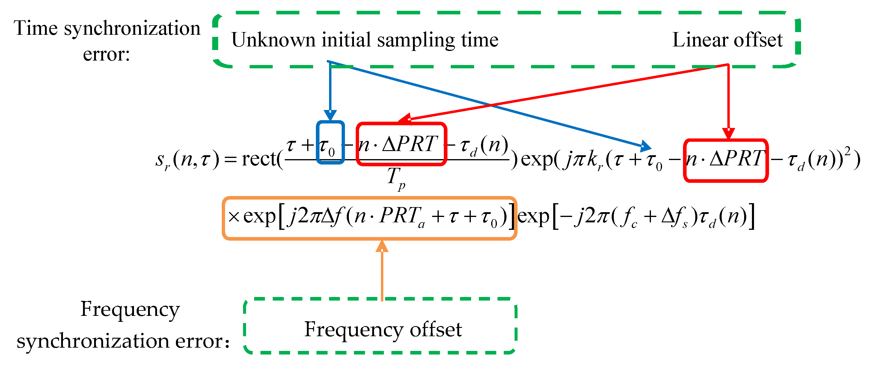
Synchronization processing is to estimate the initial sampling time, correct the linear offset, and the frequency offset of transmitting and receiving carrier frequencies. The direct wave signal after coarse synchronization is processed by pulse compression to obtain the peak position history of direct wave, and the Doppler center frequency and initial sampling distance can be estimated. According to the estimated value of the Doppler center frequency, the time synchronization error and the frequency synchronization error can be calculated. The expression of the synchronization error is shown in Figure 6.
After the synchronization error is estimated, the time and frequency synchronization error can be compensated according to the expression of the synchronization error in the signal: (1) Time synchronization: for the n -th pulse, shift n Δ P R T time to the left and (2) frequency synchronization: for the n -th pulse, multiply by phase exp [ j 2 π Δ f ( n P R T a + τ + τ 0 ) ] .
Azimuth synchronization information can also be extracted from the direct wave signal. The azimuth of the radar transmitter is estimated by the strongest pulse peak corresponding to the antenna of the transmitting station T x pointing directly to the receiving station R x . In the first few rounds of antenna scanning, the transmitted direct pulse train is sent to the azimuth synchronizer, and the average value of the antenna scanning period T N is measured as the predicted value of the next antenna scanning period. This method is suitable for the situation that the antenna of the transmitting station rotates at a uniform speed.

2.5.3. Signal Detection in Surveillance Channel

Signal detection in a surveillance channel mainly includes pulse compression, direct wave interference suppression, non-coherent integration, MTI processing/MTD processing, clutter map processing, and adaptive CFAR detection. The main procedures are summarized as follows:
  • Pulse compression: Pulse compression is accomplished by correlating the reference signal with the received target signal in the scattered echo. The reconstruction of the reference signal can be completed by the improved constant modulus algorithm and multimode algorithm (improved CMA+MMA) mentioned above. For the sake of algorithm simplicity, the pulse signal with the highest signal-to-noise ratio (SNR) in the received signal can also be directly selected as the reference signal sample.
  • Direct wave interference suppression: According to the time-domain separation characteristics of pulse signals, direct wave interference is divided into two cases: one is that the time-domain of direct wave and target echo do not overlap, and the other is that of time-domain overlap. In the first case, the time window technology is proposed to eliminate the direct wave interference. In the second case, the adaptive cancellation technique is considered to suppress the direct wave interference. The adaptive filter can adopt different adaptive algorithms. The function of these algorithms is to adjust the weighting of the filter according to the input signal and output error signal, so that the output signal of the filter is closest to the interference signal, and complete the process of adaptive interference cancellation through the cancellation of the subtractor. In the actual design of the system, the adaptive filter adopts least mean square (LMS) filter, least square (RLS) filter, and so on.
  • Non-coherent integration: When the non-cooperative radar emitter antenna scans and points to the target, the echo that is received by the surveillance channel of the receiving station is a high-frequency pulse train signal. In order to improve the detection performance of the system, the echo pulse train is usually integrated. After multi-pulse integration, the signal-to-noise ratio of the surveillance channel is improved, which is conducive to small target detection. Although the effect of non-coherent integration is not as good as coherent integration, the implementation of non-coherent integration is relatively simple and there are no strict coherence requirements for the system. Therefore, non-coherent integration is still used in many practical applications. Non-coherent integration is used to accumulate the envelope amplitude of the echo signal of the same distance unit for adjacent N repetition periods. In the actual design of the system, the small sliding window detection method is used for non-coherent integration. The window length L of the small sliding window detector is generally 5~7.
  • MTI/MTD processing: In case of strong clutter, bistatic radar can also use moving target processing equipment to detect small targets at sea. The main purpose of moving target display (MTI) technology is to enhance the target detection ability of radar and display moving targets. In the actual design of the system, three adjacent pulse cancellation plus cascaded adaptive cancellation methods are used to display moving targets. When only the dual-mode clutter (only two kinds of clutter with different velocities) is considered, because the ground clutter filter has basically filtered out the ground clutter, the cascaded adaptive filter only suppresses another kind of moving clutter (sea clutter). The main purpose of moving target processing (MTD) technology is to obtain the Range-Doppler map (R-D map) of moving targets. In the actual design of the system, the moving target processing (MTD) is carried out by FFT processing of the pulses with multiple adjacent pulse repetition periods, which is equivalent to the coherent integration of the echo pulse train.
  • Clutter map processing: This divides the whole detection area into several clutter map units. For each unit, it uses its own limited echo input to iterate repeatedly to obtain the detection threshold at the unit. Finally, the target echo in a certain detection area can be detected by the preset detection threshold of the clutter map unit. Clutter map cancellation is realized by subtracting the echo signal from the clutter map storage unit. For stationary clutter, the clutter average value of the clutter map storage unit is basically the same as that of echo, and there is basically no residue after cancellation. For a moving target that is not in the same azimuth distance unit during two antenna scans, the moving target value of the clutter map storage unit makes little contribution to the establishment of the clutter map after being averaged. Therefore, there is a large residual echo of the moving target after cancellation, so the stationary clutter can be cancelled to detect the moving target. In the actual design of the system, two time-domain clutter detection techniques, mean clutter map (ME-CM) and single pole feedback clutter map (SPFB-CM), are used.
  • CFAR detection: The detection performance of maritime targets under the background of bistatic sea clutter is easily affected by two aspects: first, when detecting at different bistatic angles, the energy distribution of sea clutter is uneven, the sea clutter is vulnerable to the clutter abnormal cell with sudden increase of power, and the false alarm rate and false detection rate are high. Second, the complex non-uniform environment that is formed by the distance sidelobes of inshore mountains, buildings, islands, and other strong scattering points makes it difficult to estimate the background power level in the formation of the CFAR detection threshold. Therefore, it is necessary to carry out adaptive CFAR detection of maritime targets under the background of bistatic sea clutter. In the actual design of the system, the cell averaging constant false alarm rate (CA-CFAR) detector and the improved variability index constant false alarm rate with abnormal cell deletion (CVI-CFAR) detector are used to detect small maritime targets.

3. Results

3.1. Experimental Scenario

Field experiments are carried out at the coastal area of the Yantai Port, China. The experimental scenario is shown in Figure 7.
There are two L-band shore-based radar transmitting coherent LFM pulse signals, which can be selected as non-cooperative radar transmitters. The parameters of non-cooperative radar transmitter 1 ( T x 1 ) are as follows: the pulse repetition frequency (PRF) is about 420 Hz, the pulse width is 160 µs, the bandwidth is about 2 MHz, the rotation speed of the radar antenna is about 6 RPM (rotation per minute) resulting in approximately 10 s scan time, and the azimuth beam width of the antenna is about 2°. The parameters of the non-cooperative radar transmitter 2 ( T x 2 ) are as follows: the pulse repetition rate (PRF) is about 450 Hz, the pulse width is 160 µs, the bandwidth is about 6 MHz, the rotation speed of the radar antenna is about 6 RPM, and the azimuth beam width of the antenna is about 2°. The HBR receiver ( R x ) is about 8 km away from non-cooperative radar transmitter 1 ( T x 1 ) and 3 km away from the non-cooperative radar transmitter 2 ( T x 2 ). The experimental targets are the ships entering and leaving the port. The maritime target area is shown in the blue shadow in Figure 7.
The physical photos of the experimental equipment are shown in Figure 8. The experimental equipment includes reference channel antenna, surveillance channel antenna, receiver and signal processor, and a PC for data processing and display. The reference antenna adopts an omnidirectional rod antenna, and the surveillance antenna adopts a directional grid antenna to point to the maritime target area to observe the scattered echo signal. The receiver and signal processor down convert the direct wave signal and the target echo signal to the baseband signal, and synchronously sample and record them in the hard disk. The PC for data processing and display completes the off-line analysis and display of the collected experimental data.

3.2. Experimental Data Acquisition

The experiments continuously collect and record the direct wave of shore-based radar and the scattering echo of maritime targets. The experimental data of the two channels are synchronously collected and recorded to the hard-disk for off-line analysis. The receiving frequency and gain of the receiver can be set by software, and the sampling rate of the data collector can also be set by software. The sampling rate range is usually 5~20 MHz. For example, for the radar with a signal bandwidth of 2 MHz, we usually set the sampling rate to 6.15 MHz. The experimental data are IQ baseband data. The data of multiple antenna rotation periods can be collected continuously according to the set sampling rate and stored in two binary files, respectively. One file is the reference channel IQ data file and the other is the surveillance channel IQ data file. The data acquisition equipment is self-developed and its photo and schematic diagram are shown in Figure 9.
The collected IQ data of the reference channel is shown in Figure 10. The data includes multiple antenna rotation periods. It can be seen that with the periodic scanning of the transmitting antenna, the received direct wave signal is periodically amplitude modulated by the transmitting antenna pattern, and the period T is about 10 s. The strongest pulse peak corresponds to the pulse that the transmitting antenna points directly to the receiving antenna.
The IQ data that were collected by the reference channel after partial magnification are shown in Figure 11 and Figure 12. It can be seen that the direct wave signal is a LFM pulse with a repetition period T r of about 2.38 ms and a pulse width τ of about 160 µs.
The time-frequency spectrum of the collected reference channel IQ data is shown in Figure 13. It can be measured that the LFM pulse signal bandwidth B is about 2 MHz. The analysis results of the collected data are consistent with the parameters of non-cooperative radar transmitter 1 that are mentioned above.
The collected IQ data of the surveillance channel is shown in Figure 14. It can be seen that t in addition to receiving the target echo, all the direct wave pulses during the rotation of the radar antenna can be received, and the received direct wave pulse may come from the side lobe of the antenna pattern.
The IQ data that were collected by the surveillance channel after partial magnification are shown in Figure 15 and Figure 16. It can be seen that the signal of the surveillance channel is obviously distorted relative to the direct wave LFM signal, which is caused by the mixing of target echo, direct wave from side lobe of antenna pattern, and clutter near the transmitting station.

3.3. Maritime Target Passive Detection and AIS Data Verification Experiment

In this experiment, the non-cooperative radar transmitter 1 ( T x 1 ) that is mentioned above is selected, and the experimental equipment that are mentioned above are used to passively detect the maritime targets entering and leaving the port. The experiment continuously collects and records the direct wave and maritime target echo data of shore-based radar. Through off-line data analysis and processing, the processing of direct wave reference signal reconstruction, time and azimuth synchronization, pulse compression, and direct wave interference suppression are completed, and the PPI-display map of HBR is drawn. At the same time, AIS ship data are recorded to dynamically track the motion state of civilian ship targets, and their position data are recorded for the verification of the experimental results of the passive detection of maritime targets. Figure 17 and Figure 18 show the comparison results between AIS map and the HBR map of maritime targets. The AIS data are used as the true value of maritime target position. Figure 19 shows the photos of the passenger ship target—BO HAI MING ZHU.
From the AIS map in Figure 17a, it can be seen that there are three passenger ships and several ships that are anchored at the anchorage in the maritime target area in Figure 7. Figure 17b is the PPI-display map of HBR at the corresponding time T1. Figure 18a is the AIS map after more than ten minutes. It can be seen that the above three passenger ships are moving away from the port. Figure 18b is the PPI-display map of HBR at the corresponding time T2. The horizontal and vertical axes represent the bistatic range samples. The horizontal and vertical axes range is ±600 (samples), and the corresponding bistatic range is about 29.5 km. It can be seen that the passive detection data of the HBR experimental system is in good agreement with the AIS data, which verifies the feasibility of the system and the correctness of the experimental results.

4. Discussion

4.1. Analysis of Moving Target Processing Results of Experimental Data

After verifying the correctness of the maritime target detection and the non-coherent processing method, it is also necessary to analyze the coherent performance of the experimental data and verify the coherent processing method that is mentioned above. As we know, under non-cooperative conditions, it is very difficult to obtain the complete coherent data of the target, and a series of synchronization technologies must be adopted, including time, frequency, and phase synchronization. With the coherent data of the targets, MTI, MTD, and other moving target processing methods can be can be applied.
Figure 20 shows one circle scanning picture of HBR map for maritime moving target detection, in which Figure 20a is a PPI display picture and Figure 20b is a range-azimuth display picture. The non-cooperative radar transmitter 2 ( T x 2 ) that is mentioned above is selected for this experiment. From the figure, we can see the ground clutter near the port and several ship targets along the port channel. The target area is marked with a black box in the figure.
Figure 21 shows the HBR map after magnification of the target area in Figure 20, in which Figure 21a is a range-azimuth map and Figure 21b is a Range-Doppler (R-D) map. As can be seen from Figure 21b, there are three targets in the target area, in which Target 1 is a moving target, and Target 1 is far away from the receiver and leaves the port because the Doppler frequency of Target 1 is negative. Target 2 and Target 3 are stationary targets because their Doppler frequency is 0 Hz. In addition, the Doppler frequency of the clutter is also 0 Hz, indicating that the clutter is a stationary clutter.
Figure 22 shows the MTI processing results of the maritime moving targets in the above target area. Among them, Figure 22a shows the original HBR map of the above target area before MTI processing, and Figure 22b shows the result after MTI processing. After MTI processing, stationary clutter and stationary targets (Target 2 and Target 3) are filtered out, and only the moving target (Target 1) is retained on the map.
The above analysis results show that the experimental data have good coherent performance, and the processing effect of MTI on moving targets is very obvious. It can be seen that it is completely feasible to use non-cooperative radar transmitter to carry out passive coherent processing on maritime targets to realize maritime moving target detection.

4.2. Analysis of Clutter Map Processing Results of Experimental Data

This section focuses on the feasibility of applying a clutter map processing method to maritime moving targets under non-cooperative conditions. The experiment needs to continuously collect and record the direct wave and maritime target echo data of multiple radar scanning cycles. Figure 23a,b and Figure 24a,b are PPI display pictures of the HBR map with four consecutive scanning cycles, respectively.
Figure 25a,b are HBR maps after the mean clutter map (ME-CM) cancellation and single pole feedback clutter map (SPFB-CM) cancellation processing, respectively.
From the experimental results of clutter map processing, the effect of the clutter map on stationary clutter cancellation is obvious, and the moving target in the map is easier to be detected after clutter map processing. The above experiment verifies the feasibility of applying a clutter map processing method to maritime moving targets by using multiple radar scanning cycle data.

5. Conclusions

In this paper, a hitchhiking bistatic radar system for maritime moving target detection is designed. The system uses the shore-based radar as the non-cooperative radar emitter. By continuously collecting the direct wave and target echo data of the non-cooperative radar, the system completes the direct wave reference signal reconstruction, pulse compression, interference suppression and synchronization processing, non-coherent integration, MTI moving target processing, clutter map processing and adaptive CFAR detection to obtain the azimuth, bistatic range and Doppler frequency of the target, and finally realizes the detection and positioning of non-cooperative maritime targets. The experiment obtained a very clear PPI display picture of HBR map, and successfully detected the ships entering and leaving the port, and the radar detection data of the experimental system is in good agreement with the AIS data. The field experiments have preliminarily verified the good detection ability of HBR for low and slow small maritime targets, and proved the feasibility of the system for maritime moving target detection.

Author Contributions

Conceptualization, J.S.; methodology, J.S.; software, Y.L.; validation, J.S. and Y.L.; formal analysis, W.X.; investigation, J.S. and W.X.; resources, W.X.; data curation, J.S. and X.C.; writing—original draft preparation, J.S. and X.C.; writing—review and editing, J.S.; visualization, Y.L.; supervision, W.X.; project administration, J.S.; funding acquisition, J.S. All authors have read and agreed to the published version of the manuscript.

Funding

This research was supported by National Natural Science Foundation of China, grant number 61971433, U1933135, 61471381, 61471380.

Data Availability Statement

Not applicable.

Acknowledgments

The authors would like to thank Caisheng Zhang and Guoqing Wang for the help of the early verification experiment.

Conflicts of Interest

The authors declare no conflict of interest.

References

  1. Kuschel, H.; O’Hagan, D. Passive Radar from History to Future. In Proceedings of the 11-th International Radar Symposium, Vilnius, Lithuania, 16–18 June 2010. [Google Scholar]
  2. Griffiths, H.D. From a Different Perspective: Principles, Practice and Potential of Bistatic Radar. In Proceedings of the International Conference RADAR 2003, Adelaide, Australia, 3–5 September 2003. [Google Scholar]
  3. Willis, N.J.; Griffiths, H.D. Advances in Bistatic Radar; SciTech Publishing Inc.: Raleigh, NC, USA, 2007; pp. 1–23. [Google Scholar]
  4. Poullin, D. Passive detection using digital broadcasters (DAB, DVB) with COFDM modulation. IEE Proc. Radar Sonar Navig. 2005, 152, 143–152. [Google Scholar] [CrossRef]
  5. Tan, D.K.P.; Sun, H.; Lu, Y. Sea and Air Moving Target Measurements Using a GSM Based Passive Radar. In Proceedings of the IEEE International Radar Conference, Arlington, VA, USA, 9–12 May 2005. [Google Scholar]
  6. Wang, Q.; Hou, C.; Long, Y. An experimental study of WiMAX-based passive radar. IEEE Trans. Microw. Theory Tech. 2010, 58, 3502–3510. [Google Scholar] [CrossRef]
  7. Colone, F.; Falcone, P.; Bongioanni, C.; Lombardo, P. WiFi-based passive bistatic radar: Data processing schemes and experimental results. IEEE Trans. Aerosp. Electron. Syst. 2012, 48, 1061–1079. [Google Scholar] [CrossRef]
  8. Mazurek, G.; Kulpa, K.; Malanowski, M.; Droszcz, A. Experimental seaborne passive radar. Sensors 2021, 21, 2171. [Google Scholar] [CrossRef] [PubMed]
  9. He, X.; Cherniakov, M.; Zeng, T. Signal detectability in SS-BSAR with GNSS non-cooperative transmitter. IEE Proc. Radar Sonar Navig. 2005, 152, 124–132. [Google Scholar] [CrossRef]
  10. Cherniakov, M.; Saini, R.; Zuo, R.; Antoniou, M. Space-surface bistatic synthetic aperture radar with global navigation satellite system transmitter of opportunity–experimental results. IET Radar Sonar Navig. 2007, 1, 447–458. [Google Scholar] [CrossRef]
  11. Dong, X.; Cui, C.; Li, Y.; Hu, C. Geosynchronous spaceborne-airborne bistatic moving target indication system: Performance analysis and configuration design. Remote Sens. 2020, 12, 1810. [Google Scholar] [CrossRef]
  12. Overrein, Y.; Olsen, K.E. Geometrical and Signal Processing Aspects Using a Bistatic Hitchhiking Radar System. In Proceedings of the IEEE International Radar Conference, Arlington, VA, USA, 9–12 May 2005. [Google Scholar]
  13. Johnsen, T.; Olsen, K.E. Hitchhiking Bistatic Radar: Principles, Processing and Experimental Findings. In Proceedings of the 2007 IEEE Radar Conference, Waltham, MA, USA, 17–20 April 2007. [Google Scholar]
  14. Strømøy, S. Hitchhiking Bistatic Radar. Master Thesis, OSLO University, Oslo, Norway, 2013. [Google Scholar]
  15. Hawkins, J.M. An Opportunistic Bistatic Radar. In Proceedings of the IEEE Radar Conference, Edinburgh, UK, 14–16 October 1997. [Google Scholar]
  16. Honda, J.; Otsuyama, T. Experimental Results of Aircraft Positioning Based on Passive Primary Surveillance Radar. In Proceedings of the 2014 Tyrrhenian International Workshop on Digital Communications, Rome, Italy, 15–16 September 2014. [Google Scholar]
  17. Hu, P.; Bao, Q.; Chen, Z. Target detection and localization using non-cooperative frequency agile phased array radar illuminator. IEEE Access 2019, 7, 111277–111286. [Google Scholar] [CrossRef]
  18. Wang, Y.; Bao, Q.; Wang, D.; Chen, Z. An experimental study of passive bistatic radar using uncooperative radar as a transmitter. IEEE Geosci. Remote Sens. Lett. 2015, 12, 1868–1872. [Google Scholar] [CrossRef]
  19. Schoenenberger, J.G.; Forrest, J.R. Principles of independent receivers for use with co-operative radar transmitters. Radaio Electron. Eng. 1982, 52, 93–101. [Google Scholar] [CrossRef]
  20. Griffiths, H.D.; Carter, S.M. Provision of moving target indication in an independent bistatic radar receiver. Radio Electron. Eng. 1984, 54, 336–342. [Google Scholar] [CrossRef]
  21. Thomas, D.D. Synchronization of Noncooperative Bistatic Radar Receivers. Ph.D. Thesis, Syracuse University, Syracuse, NY, USA, 1999. [Google Scholar]
  22. Song, J.; Cai, F.; Zhang, C.; He, Y. Experimental results of maritime moving target detection based on passive bistatic radar using non-cooperative radar illuminators. J. Eng. 2019, 20, 6763–6766. [Google Scholar]
Figure 1. Typical hitchhiking bistatic radar (HBR) system.
Remotesensing 14 03611 g001
Figure 2. Geometrical relationship of HBR system.
Remotesensing 14 03611 g002
Figure 3. Contour of the target echo power: (a) L = 20 km; (b) L = 40 km.
Remotesensing 14 03611 g003
Figure 4. Target location method of HBR system.
Remotesensing 14 03611 g004
Figure 5. Signal processing flow chart of the HBR system.
Remotesensing 14 03611 g005
Figure 6. The expression of the synchronization error.
Remotesensing 14 03611 g006
Figure 7. Scenario of the field experiment.
Remotesensing 14 03611 g007
Figure 8. The physical photos of the experimental equipment.
Remotesensing 14 03611 g008
Figure 9. Data acquisition equipment: (a) photo; (b) schematic diagram.
Remotesensing 14 03611 g009
Figure 10. The collected IQ data of the reference channel with multiple antenna rotation periods.
Remotesensing 14 03611 g010
Figure 11. The collected IQ data of the reference channel with multiple pulse repetition periods after partial magnification.
Remotesensing 14 03611 g011
Figure 12. The collected IQ data of the reference channel with single direct wave pulse after partial magnification.
Remotesensing 14 03611 g012
Figure 13. Time-frequency spectrum of the collected IQ data of the reference channel with single direct wave pulse after partial magnification.
Remotesensing 14 03611 g013
Figure 14. The collected IQ data of the surveillance channel with multiple antenna rotation periods.
Remotesensing 14 03611 g014
Figure 15. The collected IQ data of the surveillance channel with multiple pulse repetition periods after partial magnification.
Remotesensing 14 03611 g015
Figure 16. The collected IQ data of the surveillance channel with single echo after partial magnification.
Remotesensing 14 03611 g016
Figure 17. Comparison of the results between the AIS map and HBR map of maritime targets (T1 time: 10:32:13, range: 29.25 km): (a) AIS map; (b) HBR map.
Remotesensing 14 03611 g017
Figure 18. Comparison of the results between the AIS map and HBR map of maritime targets (T2 time: 10:45:02, range: 29.25 km): (a) AIS map; (b) HBR map.
Remotesensing 14 03611 g018
Figure 19. Photos of the target—BO HAI MING ZHU: (a) Docked in the port; (b) Leaving the port.
Remotesensing 14 03611 g019
Figure 20. Original HBR map for maritime moving target detection: (a) PPI display; (b) Range-azimuth display.
Remotesensing 14 03611 g020
Figure 21. HBR map after magnification of the target area: (a) Range-azimuth map; (b) Range-Doppler (R-D) map.
Remotesensing 14 03611 g021
Figure 22. HBR map of the target area before and after MTI processing: (a) Before MTI processing; (b) After MTI processing.
Remotesensing 14 03611 g022
Figure 23. HBRmap for maritime moving target detection: (a) First circle; (b) Second circle.
Remotesensing 14 03611 g023
Figure 24. HBR map for maritime moving target detection: (a) Third circle; (b) Fourth circle.
Remotesensing 14 03611 g024
Figure 25. HBRmap after clutter cancellation processing: (a) ME-CM; (b) SPFB-CM.
Remotesensing 14 03611 g025
Table 1. Typical working parameters of the HBR system.
ParametersValue
Transmitter   peak   power   ( P T )10 kw
Transmitter   antenna   gain   ( G T )30 dB
Antenna   sidelobe   gain   ( G S )−50~−20 dB
Radar   wavelength   ( λ )3 cm
Transmission   loss   ( l T )5 dB
Receiver   antenna   gain   ( G R )30 dB
Receiver   bandwidth   ( B n )10 MHz
Receiver   noise   figure   ( F n )5 dB
Reception   loss   ( l R )5 dB
Target   bistatic   radar   cross   sec tion   ( σ )10 m2
Publisher’s Note: MDPI stays neutral with regard to jurisdictional claims in published maps and institutional affiliations.

