Sensing the Urban Environment by Automotive SAR Imaging: Potentials and Challenges

Abstract

In this paper, we discuss the possibility of generating high-resolution mapping of urban (or extra-urban) environments by the application of synthetic aperture radar (SAR) processing concepts to the data collected by mm-wave automotive radars installed on-board commercial vehicles. The study is motivated by the fact that radar sensors are becoming an indispensable component of the equipment of modern vehicles, being characterized by low cost, good performance, and affordable processing; therefore, in the future, nearly every single vehicle could be potentially equipped with radar devices capable of high-resolution imaging, enabled by application of SAR processing methodologies. Throughout this paper, we aim to discuss the role of SAR imaging in the automotive context under a theoretical and experimental perspective. First, we present the resulting benefits in terms of angular resolution and signal-to-noise ratio. Then, we discuss relevant technological aspects, such as suppression of angular ambiguities, fine estimation of platform motion, and SAR processing architectures, and we present a preliminary evaluation of the required computational costs. Finally, we will present a number of experimental results based on open road campaign data acquired using an 8-channel MIMO radar at 77 GHz, considering the cases of side-looking SAR, forward SAR, and SAR imaging of moving targets.

1. Introduction

The advent of fully autonomous driving (AD), foreseen for 2030, is expected to revolutionize the automotive industry towards a safe and efficient driving experience. AD can be conceptually and technologically split into six different levels [1]. Levels from 0 to 2 involve a loose usage of onboard sensors for basic functionalities aimed at assisting the human driver, e.g., emergency braking, lane changing detection, etc. At higher AD levels, the vehicle is in charge of most of the operations concerning the driving, in any circumstance. Over the next decade, the paradigm shift will require autonomous vehicles to be able to accurately and reliably perceive the environment, in order to take real-time decisions and drive over all conditions. The reliability is the most challenging issue, as the largest part of car accidents are caused by human errors [2]. In this setting, it is widely acknowledged that the needed reliability can be achieved by sensing at both the vehicle level and network level. Network-level sensing is the ultimate goal, but enhancing the sensing capabilities of the single vehicle is the first necessary step towards AD, using multiple heterogeneous sensors [3]. Cameras, LiDARs, and radars are vital technologies for environment perception in the AD context, as they provide a multi-modal image of the surroundings. Cameras provide high-resolution images of the surrounding; deep learning techniques enable the detection and classification of objects [4]. LiDARs are active devices working in the infrared portion of the EM spectrum (800–1550 nm of wavelength), capable of providing point clouds, i.e., distance maps, of the environment [5]; however, any optical sensor (both active and passive) is sensitive to adverse weather conditions, mostly fog, challenging its stand-alone usage for safety critical applications. Automotive-legacy MIMO radars working at mm-wave (76–81 GHz [6]) are widely employed to obtain measurements of radial distance, velocity, and angular position of remote targets at comparably low cost in any weather condition, without external sources of illumination [7,8]. Current imaging performance mass-market automotive radars in terms of spatial resolution and signal-to-noise ratio (SNR) may vary depending on how data are processed, but are essentially determined by the number of antenna pairs, or channels, that form the real or virtual array. For typical automotive MIMO radars, the angular resolution is >1 deg [9]. Increasing the number of channels, thus the physical footprint of the radar, is a trivial way to improve resolution at the price of an exploding hardware cost (especially at mm-waves) with a questionable trade-off with the imaging capabilities.

A different approach is provided by synthetic aperture radar (SAR) imaging, largely employed for Earth observation and high-resolution mapping [10,11]. In essence, the SAR concept consists of exploiting the natural motion of the platform where the radar is installed to synthesize an array (aperture) of an arbitrary length. In the case of automotive mm-wave radars, SAR processing can be used to obtain a synthetic aperture of tens of centimeters or even meters, therefore producing a much finer spatial resolution than using a physical array, as well as improved SNR due to the longer observation time. Recent technological advances concerning array design, analog-to-digital conversion, and increased on-board computational resources make it possible to implement advanced signal processing techniques in real time and with low power cost [8]. The appeal exerted by this concept in the automotive scenario is well represented by the research carried out by many research groups in the last few years.

One of the first works concerning SAR in the automotive environment is the experiment carried out in [12]. In this contribution, a 300 GHz radar with 40 GHz of bandwidth was used to generate ultra-high-resolution SAR images of the urban environment, showing the capabilities of wideband SAR in mapping the urban scenario at the price of a high computational and substantially unpractical manufacturing cost for real-time mass-market deployments. In [13], the authors performed some experiments using a 77 GHz side-looking radar at 1 GHz of bandwidth. The generated SAR images map the urban environment with a resolution of 15 cm by driving on a straight path at a relatively low speed. The well-known range-Doppler focusing has been applied along a straight urban trajectory in [14], again with a side-looking configuration. Contributions [15,16] report in-lab tests carried out using a forward-looking radar combining scene scanning, synthetic aperture processing, and compressive sensing to enhance the angular resolution. A residual motion compensation scheme has been implemented in [17] with a particular focus to vehicle-based SAR images. As we explain in the following sections, autofocus plays a fundamental role in forming high-resolution images. In [18], the authors proposed a complete end-to-end algorithm composed of a pre-detection of relevant targets in the scene and a subsequent SAR image formation using time domain back projection, leading to very high angular resolution. The workflow also includes a residual motion compensation step. The work in [19] considers the role of angular diversity in SAR images, revealing some non-isotropic effects of typical urban targets. Finally, the works in [20,21] highlight the mapping capabilities of SAR imagery, with the possibility of detecting even small details as well as street conditions.

Most of these works focus on the description of a particular set-up, processing architecture, or experimental demonstration. In contrast, the scope of this paper is to consider the application of SAR imagery in the automotive scenario from a more general point of view. As discussed above, it is expected that next-generation vehicles will be equipped with radar devices and on-board processing capabilities. Accordingly, the use of SAR processing methodologies could be systematically adopted to provide radar images of the external environment with unprecedented imaging quality. In this context, we present in this paper theoretical and experimental arguments supporting of concept of automotive SAR imaging for high-resolution mapping of urban environments, and we discuss the most relevant technological aspects underpinning practical implementation. Accordingly, this paper is structured as follows. Section 2 is devoted to introducing all necessary mathematical models and notations for the understanding of the developments in this paper. The benefit of automotive SAR imaging in terms of angular resolution and SNR are discussed in Section 3. Relevant technological aspects are discussed in Section 4. In Section 5, we present experimental results based on open road campaign data acquired using an 8-channel radar at 77 GHz, considering the cases of side-looking SAR, forward SAR, and SAR imaging of moving targets. Finally, conclusions be drawn in Section 6.

2. Mathematical Model and Definitions

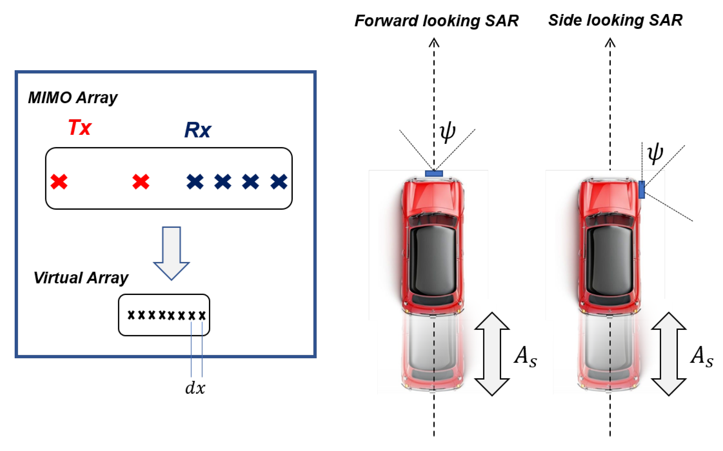
This section is intended to briefly recall data models and processing methods necessary for the understanding of the developments of this paper in later sections. As in large part of the literature on automotive radars, we assume here a typical MIMO device, where a number of transmitting (Tx) and receiving (Rx) antennas are deployed so as to form a uniformly spaced virtual array [22]. Any given pair of Tx/Rx antennas are hereafter referred to as virtual channel (or simply channel). The MIMO array is assumed to be installed on a vehicle, commonly referred to as ego-vehicle in the automotive literature, to observe the scene ahead or to the side, as sketched in Figure 1. The device is assumed to operate by transmitting pulses at a rate called pulse repetition frequency (PRF), and to store the echos received at all channels before transmitting the next pulse.

A suitable model to represent the acquired data from a single target after range compression is given as follows:

$$d_n\left(t,\tau \right)=g\left(t-{\Delta }_n\left(\tau ;{\mathit{r}}_{\mathbf{0}}\right)\right)·exp\left(-j2\pi f_0{\Delta }_n\left(\tau ;{\mathit{r}}_{\mathbf{0}}\right)\right)$$

(1)

where:

• $d_n\left(t,\tau \right)$ denotes the range-compressed signal at the n-th channel (i.e., any given pair of Tx/Rx antennas),
• $\tau$ is slow time, used to denote pulse transmission time,
• t is fast time, used to gauge delays with respect to the pulse transmission time,
• $g\left(t\right)$ is a short base-band pulse with bandwidth B,
• $f_0$ is the carrier frequency,
• ${\Delta }_n\left(\tau ;{\mathit{r}}_{\mathbf{0}}\right)$ is the total delay from the target at position ${\mathit{r}}_{\mathbf{0}}$ to the positions of the Tx and Rx antennas that form the n-th channel at time $\tau$, here defined as ${\mathit{s}}_l^{Tx}$ and ${\mathit{s}}_m^{Rx}$, where l and m are the indexes of the transmitting and receiving real elements:

  $${\Delta }_n\left(\tau ;{\mathit{r}}_{\mathbf{0}}\right)=\frac{1}{c}\left(∥{\mathit{s}}_l^{Tx}\left(\tau \right)-{\mathit{r}}_{\mathbf{0}}∥+∥{\mathit{s}}_m^{Rx}\left(\tau \right)-{\mathit{r}}_{\mathbf{0}}∥\right)$$

  (2)

It is worth noting that the waveform $g\left(t\right)$ in (1) is the resulting waveform after range compression, and is therefore assumed to be a short signal of effective duration $1/B$. For automotive radars, the transmitted (i.e.: before range compression) waveform is typically much longer, on the order of few tens of microseconds for typical frequency modulated continuous wave (FMCW) transmission schemes, see for example [13,14]. Further note that in Model (1), we implicitly assume that any residual phase term associated with the FMCW reception scheme has been compensated for [23]. This assumption is not strictly necessary, nor critical, for the developments to follow, and is here only retained to simplify the notation and improve the readability of the paper. SAR image formation, usually referred to as focusing, can be carried out under different approaches, which may largely differ concerning both underlying assumptions and computational costs, see for example [24,25,26]. Within this section, we assume image formation by time domain backprojection (TDBP), which is known in the literature as an exact algorithm for SAR imaging and is therefore considered as the reference method [26]. Following Model (1), the back-projection operator is expressed as:

$$I\left(\mathit{r}\right)=\sum _{\tau }\sum _n{d}_n\left(t={\Delta }_n\left(\tau ;\mathit{r}\right),\tau \right)·exp\left(+j2\pi f_0{\Delta }_n\left(\tau ;\mathit{r}\right)\right)$$

(3)

where:

• $I\left(\mathit{r}\right)$ is the focused SAR image,
• $\mathit{r}$, which we refer to as focusing grid, represents the spatial position associated with any pixel of the focused SAR image,
• $d_n\left(t,\tau \right)$ is the range-compressed data described in (1),
• ${\Delta }_n\left(\tau ;\mathit{r}\right)$ is the total delay from the grid position $\mathit{r}$ to the positions of the Tx and Rx antennas that form the n-th channel at time $\tau$.

The synthetic aperture, hereafter indicated with $A_s$, is defined as the length traveled by the sensor during the time it took to acquire the data used to form an SAR image (typically few tens of cm for a 77 GHz automotive sensor). Accordingly, automotive SAR imaging can be thought of as the result of a coherent integration along two different apertures, one represented by the virtual array of the MIMO device, and one synthesized by the motion of the ego-vehicle. It is interesting to note that (3) describes three specific operations. The first one is an interpolation, represented by the notation $t={\Delta }_n\left(\tau ;\mathit{r}\right)$ within the argument of $d_n\left(t,\tau \right)$. This operation allows us to read the raw data at a specific time instant as a function of grid position, slow time, and virtual channel, so as to keep track of the variation of the delay of any target within the focusing grid. In doing so, the focusing algorithm manages to account for range migration, that is for any variation of a target delay (or range, equivalently) in excess of one time bin. The second operation carried out in (3) is a phase rotation, which again is allowed to vary depending on grid position, slow time, and virtual channel. This operation allows us to account for the exact law of variation of the wave phase across different channels and different pulses, which includes the wave-front curvature as well as any possible effect that arises when platform trajectory is not straight or uniform. The third operation consists in accumulating the interpolated and phase-rotated data over all channels and pulses. Importantly, the sum over n and $\tau$ in (3) can be split to yield:

$$I\left(\mathit{r}\right)=\sum _{\tau }{I}_s\left(\mathit{r};\tau \right)$$

(4)

where $I_s\left(\mathit{r};\tau \right)$ are referred to as sub-images, and represent low-resolution MIMO images obtained by back-projecting the data associated with the transmission of a single pulse at time $\tau$, that is:

$$I_s\left(\mathit{r};\tau \right)=\sum _n{d}_n\left(t={\Delta }_n\left(\tau ;\mathit{r}\right),\tau \right)·exp\left(+j2\pi f_0{\Delta }_n\left(\tau ;\mathit{r}\right)\right)$$

(5)

As a final remark, it is worth here commenting on the key role played by the delay ${\Delta }_n\left(\tau ;\mathit{r}\right)$ in (3) and (5). In the first place, any mismatch in the calculation of delays, as for example those resulting from an erroneous knowledge of the vehicle trajectory, results in a wrong phase correction, and therefore in a degradation of image contrast and arising of side-lobes [27]. For this reason, SAR processing needs to be flanked by an accurate estimation of platform trajectory, as we discuss in Section 4. Moreover, the calculation of delays requires a preliminary choice about reference frame in which the motion takes place. For SAR, it is customary to consider a fixed reference frame in which the targets are not moving, resulting in SAR images of static targets; however, the back-projection algorithm in (3) can be seamlessly used to image moving targets as well, simply by calculating the delays in a new (and typically non-inertial) reference frame in which the targets are stationary, as we show in Section 5.

3. The Benefits of Automotive Synthetic Aperture Radar

In this section, we discuss how SAR processing contributes to improving image quality with respect to conventional radar imaging. The discussion is articulated in a quantitative manner by considering the resulting spatial resolution and SNR, as such parameters ultimately convey the capability of an imaging system to detect and localize a target in a noisy environment and/or in the presence of other closely spaced targets.

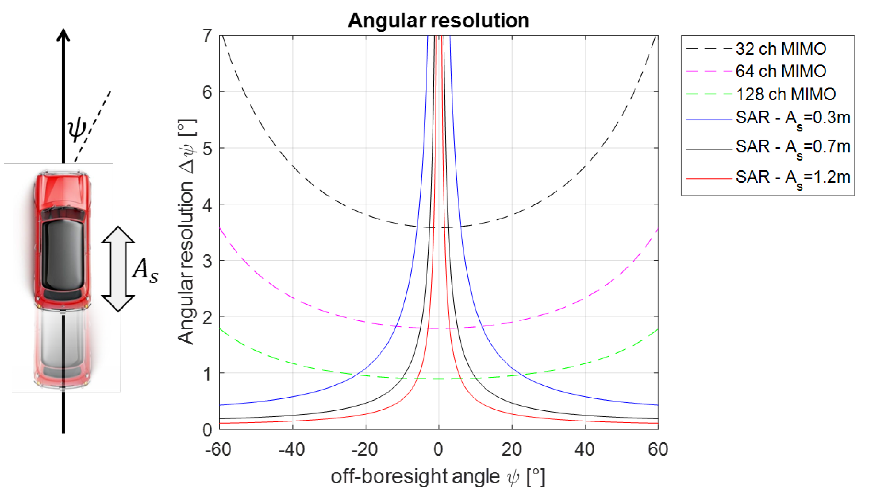
For a typical MIMO imaging radar, both resolution and SNR are largely determined by the number of channels within its virtual array. As discussed above, we consider the typical case where Tx and Rx antennas form a uniformly spaced virtual array [22], in which case the angular resolution is readily obtained as the ratio of wavelength to twice the effective array aperture. Assuming the customary forward-looking installation, one has:

$$\Delta {\psi }_{MIMO}=\frac{\lambda }{2cos\left(\psi \right)}·\frac{1}{N_{ch}dx}$$

(6)

where $\lambda$ is the carrier wavelength, $N_{ch}$ is the total number of available virtual channels, $dx$ is the spacing between nearby elements in the virtual array (assuming the virtual array is represented as a collection of monostatic elements), and $\psi$ is the off-boresight angle, as shown in Figure 2.

In the vast majority of cases, the antenna layout is such that $dx=\frac{\lambda }{4}$ to ensure non-ambiguous imaging, after which one has that angular resolution is fully determined by the geometrical factor $cos\left(\psi \right)$ and the number of elements $N_{ch}$. For any value of $dx$, the product $N_{ch}dx$ represents the length of the virtual array in Figure 1, which is upper-bounded by the physical size of the sensor. Figure 2 shows the variation of angular resolution, as obtained according to (6), for the cases of a MIMO array with 32, 64, or 128 channels.

In the case of SAR imaging, resolution is achieved by processing a chunk of data acquired as the vehicle travels the length $A_s$, which can be thought of as the length of an equivalent (monostatic) virtual array deployed longitudinally. Accordingly, the angular resolution for SAR imaging is obtained as:

$$\Delta {\psi }_{SAR}=\frac{\lambda }{2sin\left(\psi \right)}·\frac{1}{A_s}$$

(7)

where the geometrical factor is now $sin\left(\psi \right)$ due to the longitudinal deployment. Comparing (6) with (7), and by Figure 2, it is immediate to see that SAR imaging can serve as a natural complement to conventional radar in the automotive context. SAR imaging does not bring any improvement for targets right at boresight; yet, it does provide a far superior resolution for targets slightly off-boresight. 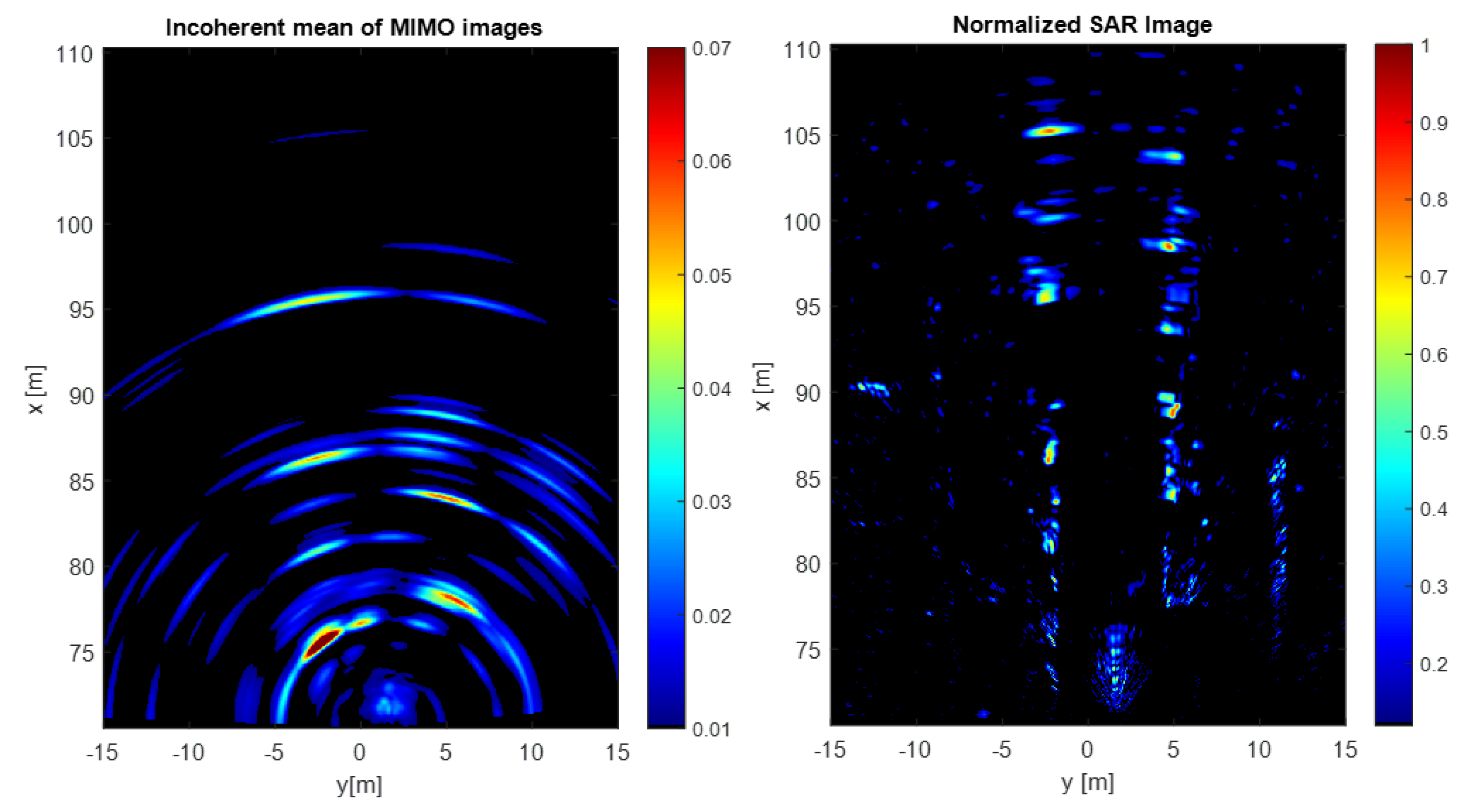Figure 3 shows of the left the incoherent mean of 256 low-resolution MIMO images. The resolution is quite poor if compared with the right image in the same figure. The latter is the SAR image obtained by coherently combining all the 256 snapshots. The improvement in resolution provided by SAR allows for an easy detection of parked cars, sidewalk, fences, and many more. We remark that these images were acquired in an open road campaign, in this case with a $PRF=7$ KHz, with the car traveling at roughly 30 km/h for a total synthetic aperture of 30 cm.

To discuss SNR for radar and SAR imaging, we simply assume some processing scheme where consecutive pulses are coherently integrated over some coherent integration time $T_c$, which is proportional to the SNR improvement factor over single-pulse data per processed channel. The effective coherent integration time depends largely on which processing scheme is adopted. As discussed in Section 2, the common trait of accurate SAR imaging algorithms is to account for any effect related to the variation of the sensor-to-target travel time across different pulses, which includes compensation of range migration and non-linear phase variations. If this is performed, the coherent integration time is only bounded by the physical antenna beam width, as it is the case for spaceborne and airborne SARs [10].

On the other hand, radar imaging is (typically) implemented under the assumptions that range migration can be neglected and phase variations are linear. Such assumptions allow for a significant simplification of the signal model and all related processing algorithms. Yet they set an upper bound for the coherent integration time. To express the upper bound quantitatively without compromising the readability of the exposition, we assume in this section that the delay in (1) can be approximated as in the case of a monostatic radar as $\Delta =\frac{2}{c}R\left(\tau \right)$, with c the wave propagation velocity and $R\left(\tau \right)$ the average distance of a target with respect to the Tx and Rx antennas in a given channel at time $\tau$ (note that this is indeed an excellent approximation as long as the MIMO array is much shorter in comparison with the distance, which is always the case for this paper).

As for range migration, the requirement to set is that delay variations do not exceed temporal resolution. Approximating the distance variation with time as being linear, the derivative of delay with respect to time is expressed as:

$$\frac{\partial \Delta \left(\tau \right)}{\partial \tau }=\frac{2}{c}\frac{\partial R\left(\tau \right)}{\partial \tau }\simeq \frac{2}{c}{v}_{ego}·cos\left(\psi \right)$$

(8)

with $v_{ego}$ the vehicle forward velocity, and $\psi$ the off-boresight angle. Requiring the delay variation not to exceed temporal resolution, one gets:

$$\frac{2}{c}{v}_{ego}·cos\left(\psi \right)·T_c<\frac{1}{B}.$$

(9)

The non-linear nature of the phase history can be accounted for by bounding the residual parabolic component of the delay. By virtue of the monostatic approximation retained in this section we have:

$$\frac{d^2\phi }{d{\tau }^2}=2\pi f_0\frac{d^2\Delta }{d{\tau }^2}=\frac{4\pi }{\lambda }\frac{d^{2}R}{d{\tau }^2}=\frac{4\pi }{\lambda }\frac{{sin}^2\left(\psi \right)}{R}{v}_{ego}^2$$

(10)

with $\lambda =\frac{c}{f_0}$ the wavelength. Setting $\frac{\pi }{2}$ as the upper threshold for the allowed phase variations we obtain:

$$\Delta \phi =\frac{1}{2}\frac{d^2\phi }{d{\tau }^2}{\left(\frac{T_c}{2}\right)}^2=\frac{\pi }{2}\frac{{sin}^2\left(\psi \right)}{\lambda R}{v}_{ego}^2{T}_c^2<\frac{\pi }{2}$$

(11)

The final upper bound on the coherent integration is readily obtained by putting together (9) and (11):

$$T_c<min\left(\frac{c}{2B·v_{ego}·cos\left(\psi \right)},\frac{\sqrt{\lambda R}}{v_{ego}·sin\left(\psi \right)}\right).$$

(12)

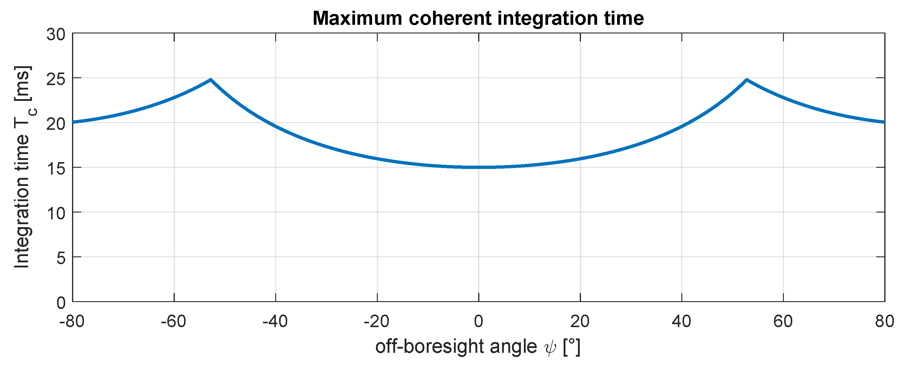
To quantify the limits on $T_c$, we assume here a set of parameters representative for high-resolution urban mapping, such as $f_0=77$ GHz, $v_{ego}=10$ m/s, $B=1$ GHz, and $R=10$ m. After (12) one finds that the coherent integration time is on the order of 20 ms for most targets, with minor variations depending on the off-boresight angle as shown in Figure 4. This value sets a physical limit to the SNR improvement factor achieved by integrating over time, unless exact SAR processing is adopted. In other words, $T_c$ is the upper limit for a coherent integration time if range migration is not compensated and if a linear phase model is adopted.

Of course, in conventional radar imaging, both SNR and angular resolution can always be improved by increasing the number of channels $N_{ch}$ that is by moving towards more sophisticated and expensive devices. On the other hand, the present analysis has just shown that SAR processing allows for large performance improvements by exploiting the natural motion of the ego-vehicle, therefore opening the way to the concept of high-resolution mapping using low-cost devices. The price to pay is obviously an increased complexity and computational burden, as we discuss in the next section.

4. Technological Aspects

This section is dedicated to discussing relevant technological aspects and challenges related to the practical implementation of automotive SAR imagery.

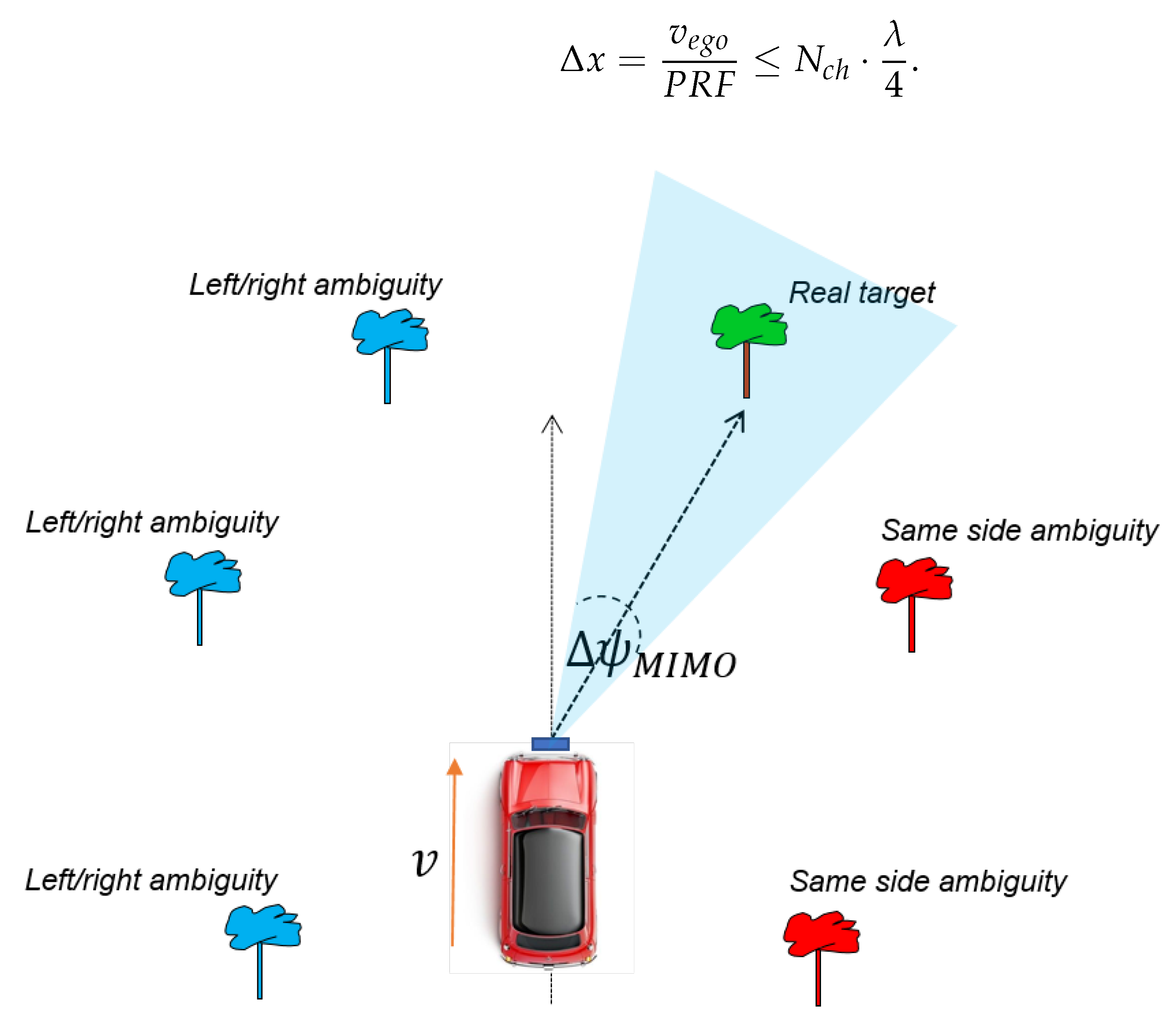
4.1. Rejection of Angular Ambiguities

A most important aspect in radar imagery is the suppression of angular ambiguities, namely spurious signals that arise due to the finite spatial sampling and that can be confused for real targets [10,11]. To discuss the matter on a quantitative basis, we define here $\Delta x$ as the distance traveled by the sensor in between two consecutive transmissions, in such a way as to form a uniformly sampled array with spacing $\Delta x$. Then, the angular positions at which ambiguities appear are obtained as the solutions of the equation:

$$cos\left({\psi }_{amb}\right)=cos\left(\psi \right)+\frac{\lambda }{2·\Delta x}·k$$

(13)

where $\psi$ is the angular position of a physical target, hereafter referred to as the real target, ${\psi }_{amb}$ is the angular position of all resulting ambiguities, and k is any integer. As a result, ambiguities in automotive SAR imagery are prone to appearing both to the same and to the opposite side of the ego-vehicle with respect to the real target, as pictorially illustrated in Figure 5.

A well-known condition to suppress same-side ambiguities in airborne SARs is to transmit pulses at a sufficiently high rate to let the spacing $\Delta x$ be no larger than a quarter of a wavelength, as in this case (13) would admit no other solution than ${\psi }_{amb}=\pm \psi$. Yet, in the case of a 77 GHz radar traveling at 20 m/s, fulfilling this requirement would result in the need for a PRF higher than 20 KHz, which is typically well beyond the capabilities of low-cost devices in terms of data throughput. A robust solution to relax this requirement while also suppressing left/right ambiguities is to use a multichannel system, as it the case of advanced SONAR and spaceborne SARs [28,29]. In few words, the principle behind ambiguity suppression by multichannel processing is that ambiguities are canceled out upon the condition that their angular distance from the real target is larger than the angular resolution of the multichannel array, as pictorially illustrated by the blueish beam in Figure 5. Discussing suppression performance over a large angular region requires careful numerical analysis to account for the radiation pattern of single antenna elements [30], and is therefore considered outside the scope of this paper. Still, an approximate condition can be stated by assuming a spacing $dx$ between nearby elements of the virtual array equal to a quarter of a wavelength, as discussed in Section 3, and under the further assumptions that array side-lobes can be neglected and the target to be imaged is stationary. In those circumstances, the maximum spacing $\Delta x$ between consecutive transmissions can be upper-bounded as:

$$\Delta x=\frac{v_{ego}}{PRF}\le N_{ch}·\frac{\lambda }{4}.$$

(14)

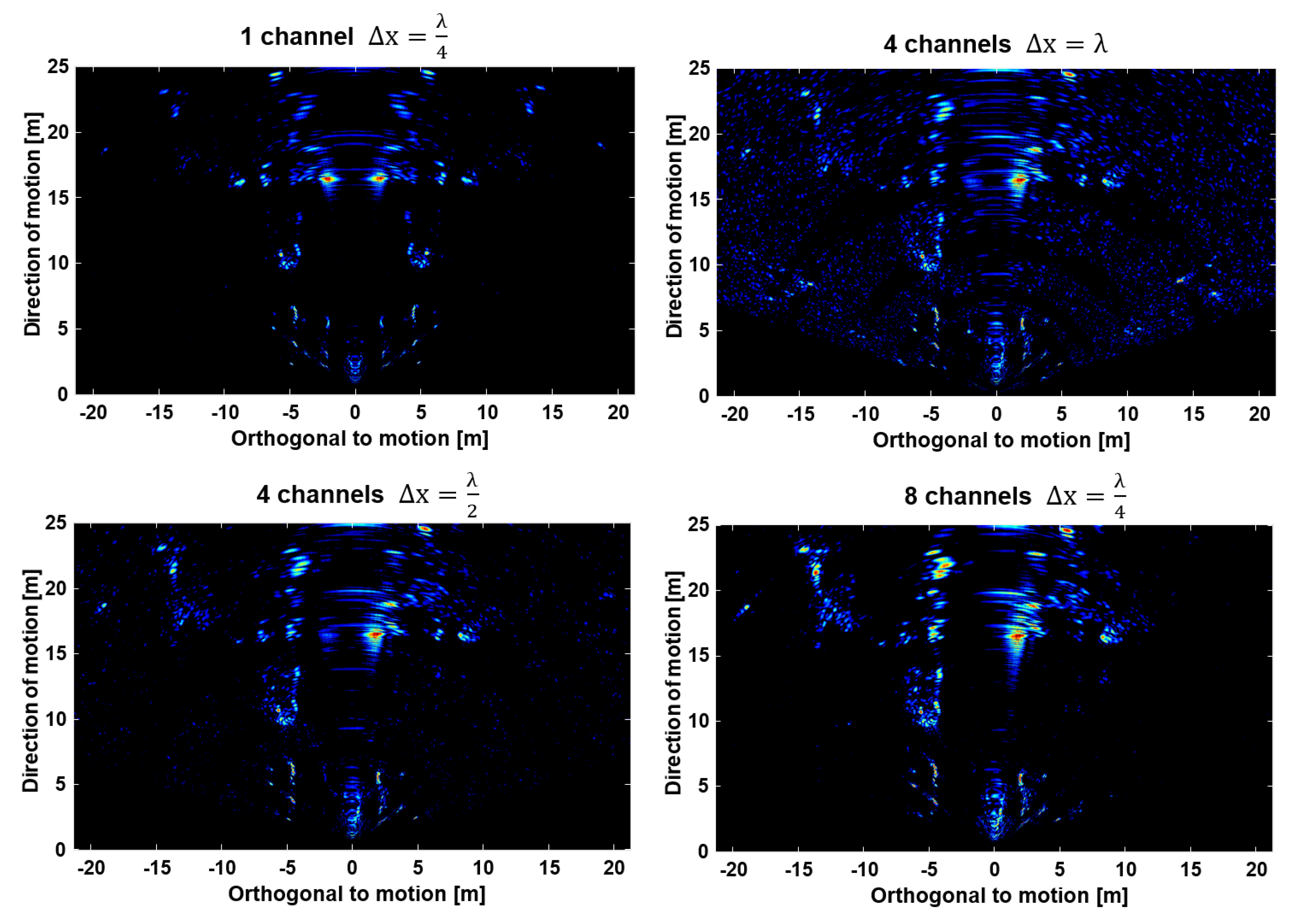
Although an approximate relation, (14) clearly states that the availability of multichannel data is key to achieving correct SAR imaging at higher speeds. For example, assuming an 8-channel device operating at 77 GHz and at a PRF of 5 KHz, (14) predicts that correct SAR imaging is possible up to a velocity of about 140 km/h. In our experience, though, the assessment in (14) is over-optimistic by about a factor of 2, resulting in the same device to be usable for SAR imaging up to a velocity of about 70 km/h. As an example, we show in Figure 6 four forward SAR images as obtained by processing the same data using a number of channels ranging from 1 to 8 and at different PRF. The image in the bottom right panel was obtained by using eight channels and by setting the PRF such that the spacing $\Delta x$ between consecutive transmissions is equal to a quarter of a wavelength. As a result, this image meets the condition in (14) with large margins, and can be taken as reference. The image in the top left panel was obtained with the same PRF, but processing a single channel. As a result, this image is contaminated by left/right ambiguities. The image in the top right panel was obtained by processing four channels and letting $\Delta x$ equal one wavelength. In doing so, this image meets the condition in (14) exactly. No ambiguity is here clearly detected; yet, the image appears to be contaminated by spurious contributions everywhere, as a result of the approximate nature of (14). A significantly better result is obtained and shown in the bottom left panel by letting $\Delta x$ equal half a wavelength. In this case, spurious contributions are strongly reduced, and imaging quality is comparable to the reference image in the bottom right panel.

4.2. Ego-Motion Retrieval

An important aspect for accurate SAR imaging is the knowledge of the platform trajectory, which should be a small fraction of a wavelength at the scale of one synthetic aperture [27]. For automotive applications, a simple condition on the accuracy of ego-velocity is derived by requiring the velocity error to be smaller than velocity resolution of the system, yielding:

$$\Delta v_{ego}<\frac{\lambda }{2T_c}.$$

(15)

with $T_c$ the coherent integration time. A velocity estimation error larger than (15) will result in a mis-localization of the target by a resolution cell. To gain insight on this condition, we consider as an example $T_c=100$ ms, after which the maximum tolerable velocity error amounts $\Delta v_{ego}=2$ cm/s. Such an accuracy is typically not met by standard navigation systems [31], and calls for a dedicated procedure to refine the platform motion estimation directly from radar data. The availability of a multichannel device greatly simplifies the task of velocity estimation, which can be carried out to within sufficient accuracy by analysis of the Doppler frequency at different off-boresight angles, see for example [18,32,33]. The idea is that if the vehicle’s trajectory is perfectly known, the TDBP properly compensates for all the distances leading to a zero residual phase over each target in the scene. If, on the other hand, the trajectory provided by the vehicle’s navigation unit is not matching the real trajectory, a residual phase term arises. The error on the estimated trajectory can be modeled as a constant velocity error. This assumption is valid over short synthetic apertures and it is the most common model in the literature [18,32,34,35]. The constant velocity error hypothesis leads to an easy expression of the residual Doppler frequency over each target in the scene:

$$f_d\left(\psi \right)=\frac{2}{\lambda }\Delta v_{ego,r}\left(\psi \right)=\frac{2}{\lambda }(\Delta v_{ego,x}cos\psi +\Delta v_{ego,y}sin\psi )$$

(16)

where $\Delta v_{ego,r}\left(\psi \right)$ is the residual radial velocity as seen by a target at angular position $\psi$, $\Delta v_{ego,x}$ is the residual velocity in the direction of motion, while $\Delta v_{ego,y}$ is the one orthogonal to motion.

The estimation of the parameters of interest ($\Delta v_{ego,x}$ and $\Delta v_{ego,y}$) can be carried out by detecting a set of N fixed ground control points (GCPs) in the scene and by retrieving the residual Doppler frequency over each of them. In this way, we obtain a linear system of equations:

$$\left[\begin{array}{c}{f}_d\left({\psi }_0\right)\\ f_d\left({\psi }_1\right)\\ f_d\left({\psi }_2\right)\\ ⋮\\ f_d\left({\psi }_N\right)\end{array}\right]=\frac{2}{\lambda }\left[\begin{array}{cc}cos{\psi }_0& sin{\psi }_0\\ cos{\psi }_1& sin{\psi }_1\\ cos{\psi }_2& sin{\psi }_2\\ ⋮& ⋮\\ cos{\psi }_N& sin{\psi }_N\end{array}\right]\left[\begin{array}{c}\Delta v_{ego,x}\\ \Delta v_{ego,y}\end{array}\right]$$

(17)

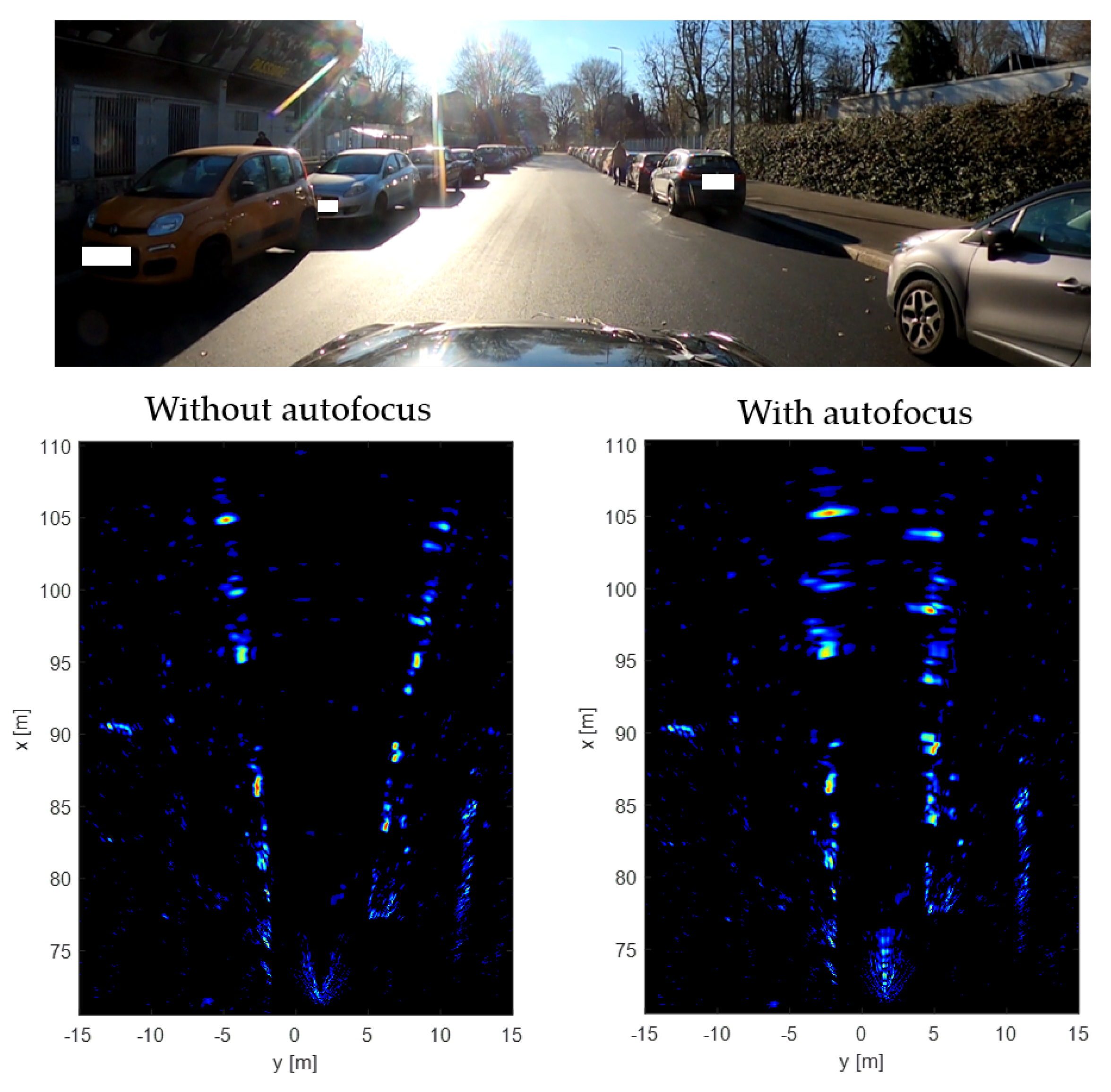
Notice that the measurement vector containing all the residual Doppler frequencies can be obtained by a simple Fourier transform of the slow-time over each detected GCP in the scene. This is the case thanks to the assumption of constant velocity error that in turn is responsible of a constant residual Doppler frequency. The design matrix is built upon the knowledge of the off-boresight position of each GCP. In this setting, a multichannel device is essential to provide an a-priori knowledge of the angular positions of the GCPs. To show the effect of a residual velocity estimation error and the corresponding impact of autofocus, Figure 7 shows two images: the first generated without employing any autofocus procedure and the second with a suitable autofocus procedure to recover residual trajectory estimation errors from navigation data with radar ones [32]. In the former, the image is corrupted and collapsed outward, not representing the true scene; it is clear that this product is useless for safety-critical automotive applications. On the other hand, the second image shows the road straighten up and the targets correctly localized in space.

4.3. SAR Processor Architecture

The discussion above allows us to draw some conclusions about the basic requirements of an automotive SAR processor:

• SAR imaging requires to exactly match the range and phase history of all targets within the radar field of view (FoV) for any motion of the ego-vehicle; therefore, the SAR processor has to account for range migration and phase curvature for both uniform and non-uniform motions.
• Multichannel processing is imperative for automotive SAR, as it is needed to suppress ambiguities at any speed.
• The SAR processor should always integrate an accurate ego-motion retrieval algorithm to fulfill the condition in (15).

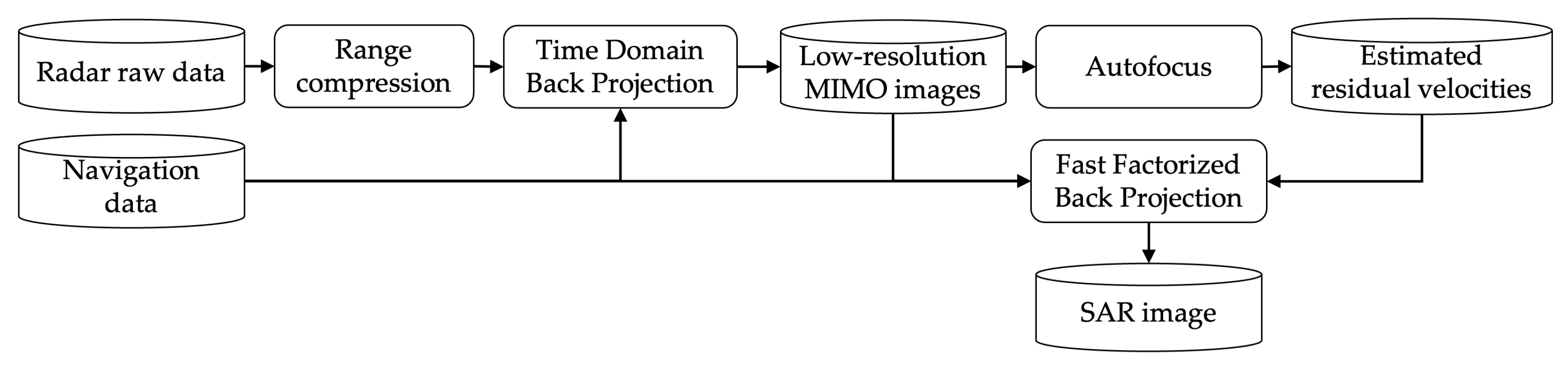
In light of these requirements, we deem the best architecture for automotive SAR processing to be based on the idea of factorized back projection (FBP) [25]. A block diagram of the complete processing scheme is depicted in Figure 8.

FBP was originally conceived out of the necessity to have a fast SAR processor that could preserve image focusing accuracy in the case of strong non-linear motions, which would invalidate the use of frequency-based approaches. For short, FBP algorithms proceed by partitioning the synthetic aperture into a number of sub-apertures, each of which is back-projected to form a low-resolution image, or sub-image. Afterwards, all sub-images are combined following a hierarchical progression to form a single high-resolution image [25]. In doing so, FBP algorithms manage to largely reduce the computational burden to within a speed-up factor well above 100, see for example [25].

This approach appears to be particularly suited to the automotive scenario since it respects all the requirements previously cited:

• It is always correctly matched to the actual motion of the ego-vehicle (errors might result from interpolation kernels, but not from approximations of the ego-motion).
• It is very easily adapted to multichannel processing: all it takes is to consider a sub-aperture as the collection of multichannel data from a single pulse, or from few pulses.
• Each of the generated sub-images represents a low-resolution snapshot where the targets are resolved in range and angle. This allows for a direct estimation of velocity by analyzing the phase variation over time at each point in the radar FoV, therefore resulting in a seamless integration of ego-motion retrieval.

4.4. Estimation of Computational Costs

In this section, we provide a preliminary assessment of the computational costs associated with SAR imaging. The discussion is proceeded by comparing two approaches, namely a direct implementation of the TDBP algorithm and a fast-factorized version (FFBP), conceptually similar to the one discussed in [25].

We start with an aperture size of $N_{\tau }$ slow-time samples, each one with $N_{ch}$ channels to be back-projected. The rough number of operations required by the classical TDBP in polar coordinates can be expressed as:

$${\mathrm{OP}}_{\mathrm{TDBP}}=\underset{\mathrm{total}\mathrm{samples}}{\underbrace{(N_{ch}\times N_{\tau })}}\times \underset{\mathrm{size}\mathrm{of}\mathrm{the}\mathrm{grid}\mathrm{in}\mathrm{angle}}{\underbrace{(N_{ch}\times N_{\tau })}}\times \underset{\mathrm{size}\mathrm{of}\mathrm{the}\mathrm{grid}\mathrm{in}\mathrm{range}}{\underbrace{N_r}}$$

(18)

Notice that the number of angular samples in the polar BP grid is proportional to the number of processed samples.

The FFBP, instead, works in stages. In the first stage, we divide the $N_{\tau }$ slow-time samples in groups, each one of size $N_{sub}$ resulting in $N_{\tau }/N_{sub}$ sub-apertures.

The stack of low-resolution images is interpolated on a new polar grid of size $N_{sub}{N}_{\psi }\times N_r$ in angle and range, respectively.

This time $N_{\psi }$ is the initial number of samples of polar BP grid that depends from the number of virtual channels ($N_{\psi }\approx 2N_{ch}$).

$$\underset{\#\mathrm{sub}-\mathrm{apertures}}{\underbrace{\frac{N_{\tau }}{N_{sub}}}}\times \underset{\#\mathrm{samples}}{\underbrace{N_{sub}}}\times \underset{\#\mathrm{angular}\mathrm{pixels}}{\underbrace{2N_{sub}{N}_{ch}}}\times \underset{\#\mathrm{range}\mathrm{pixels}}{\underbrace{N_r}}$$

(19)

In the second stage, the size of the sub-apertures remains the same, the number of sub-apertures lower by a factor $N_{sub}$ becoming $N_{\tau }/N_{sub}^2$, while the size of the polar BP grid increases by a factor $N_{sub}$ to account for the improvement in resolution, becoming $2N_{sub}^2{N}_{ch}$. It is now clear that the second stage has the same number of operations as the first one. The same reasoning can be applied recursively for all the steps.

The number of stages is roughly ${log}_{N_{sub}}{N}_{\tau }$; therefore, the total number of operations for the FFBP is

$${\mathrm{OP}}_{\mathrm{FFBP}}=N_{\tau }{log}_{N_{sub}}{N}_{\tau }\times 2N_{sub}{N}_{ch}\times N_r$$

(20)

Accordingly, the computational gain with respect to the TDBP is proportional to:

$$\frac{{\mathrm{OP}}_{\mathrm{TDBP}}}{{\mathrm{OP}}_{\mathrm{FFBP}}}\propto \frac{N_{\tau }{N}_{ch}}{2N_{sub}{log}_{N_{sub}}{N}_{\tau }}$$

(21)

As an example, assuming $N_{ch}=8$ channels, $N_{\tau }=256$ slow-time samples, and a sub-aperture size of $N_{sub}=4$ samples, the computational gain is equal to 64, whereas with 512 slow-time samples it increases to 113.

Equation (20) was used as the denominator in Equation (21) to provide a rough gain factor of the FFBP compared to the direct TDBP; however, if we want to give a more accurate figure for the number of operations requested to form an SAR image, we have to consider also all the mathematical operations at every stage of the FFBP, including demodulation, interpolation, modulation, and coherent integration.

An absolute figure can be then provided if we multiply Equation (20) by a factor K that accounts for all these mathematical operations. In our experience, the factor K is roughly 12. If we now consider also the range compression, the number of operations approaches half a billion for each image. For comparison, a 9-year-old iPhone®5S has a raw processing power of 76 GigaFlops [36], meaning it could focus an SAR image in some 7 ms.

5. SAR Imaging of an Urban Scenario

This section illustrates a few results from two open road acquisition campaigns in Milan. All data were acquired using a ScanBrick^® FMCW MIMO radar developed by Aresys based on the AWR1243 single-chip by Texas Instruments [37]. The ScanBrick^® features up to 12 channels ( four of which were for interferometric purposes, which we did not use), a large field of view (above $\pm 50$ deg), flexibility of operation mode, and, most importantly, full access to raw data. The ScanBrick^® was installed onboard an Alfa Romeo Giulia Veloce in two configurations: (i) on the right side of the hood to look sideways, and (ii) on the front grid to look forward. Side-looking data were acquired by operating the radar to continuously transmit chirp pulses with a bandwidth of 3.7 GHz at a PRF = 1 KHz, to allow for non-ambiguous imaging at a maximum velocity of approximately 15 km/h (after (14)), and accounting for some margin). Forward-looking data were acquired by operating in burst mode, with a burst duration $T_b=37$ ms and a duty cycle of 50%, and transmitting chirp pulses with a bandwidth of 1 GHz. The PRF in this second case was about 7 KHz, after we expect unambiguous imaging up to about 100 km/h. SAR processing was implemented via a multichannel FBP scheme as previously described. The radar equipment was complemented by a navigation sensor rigidly mounted on top of the radar, providing the coarse trajectory estimation. The sensor is a relatively low-cost (automotive-grade) inertial navigation solution integrating a 3D accelerometer, a 3D gyroscope, and a global navigation satellite system (GNSS) sensor. In addition, the car was equipped with a camera to visually cross check the generated images.

5.1. Side-Looking SAR

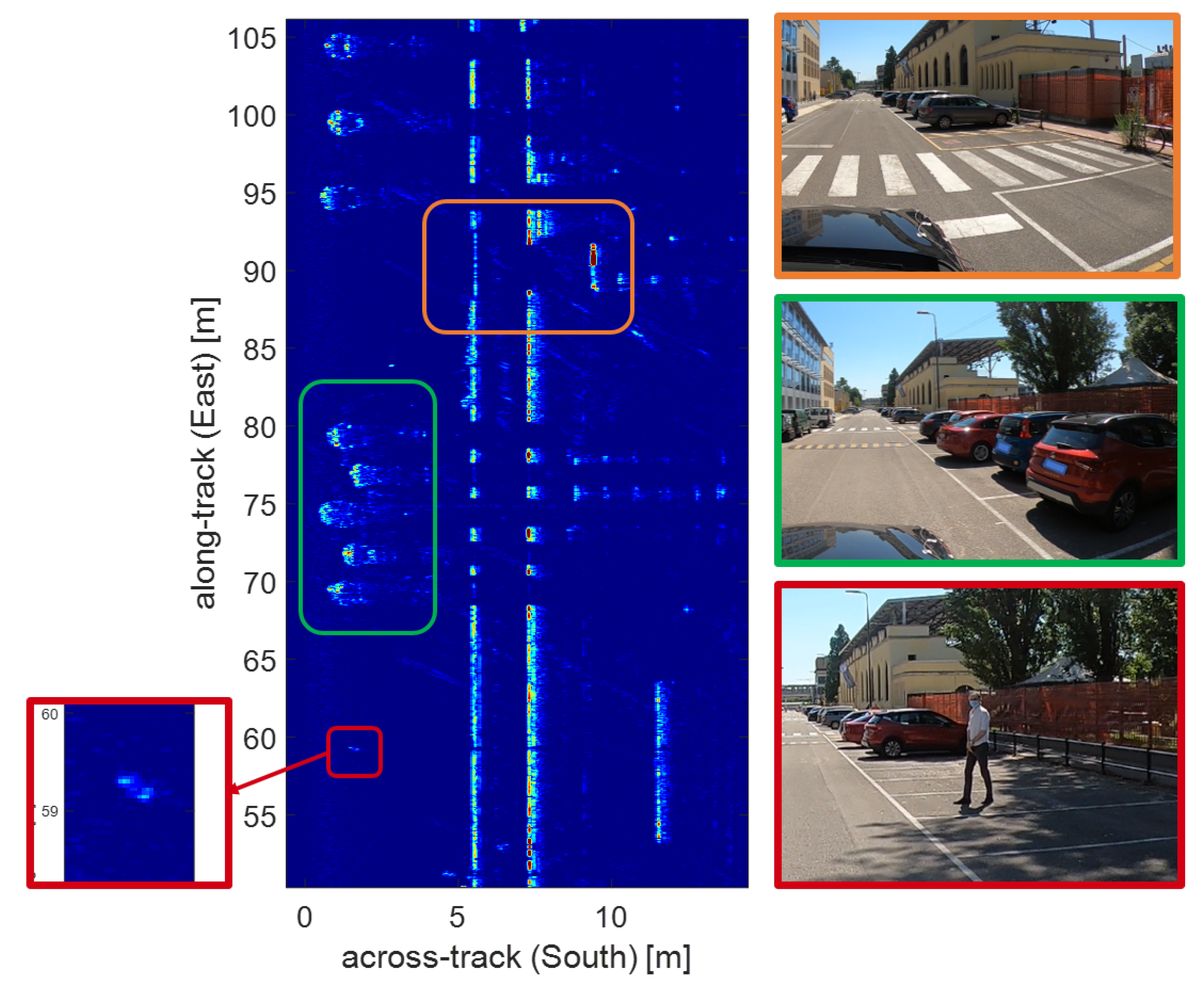
An example of side-looking SAR is shown in Figure 9. On the left an SAR image formed over a 60-m-long track is shown. This image was produced by varying the synthetic aperture length with range to achieve a uniform along-track resolution. It is easy to recognize the parked cars in the green box, which appear as very bright targets. Interestingly, the dihedral reflection from the sidewalk is also clearly detected, as highlighted in the orange box, along with a metallic fence.

Another interesting target is the standing pedestrian in the red box. In this case, the resolution is so fine that it is easily possible to recognize his posture.

5.2. Forward-Looking SAR

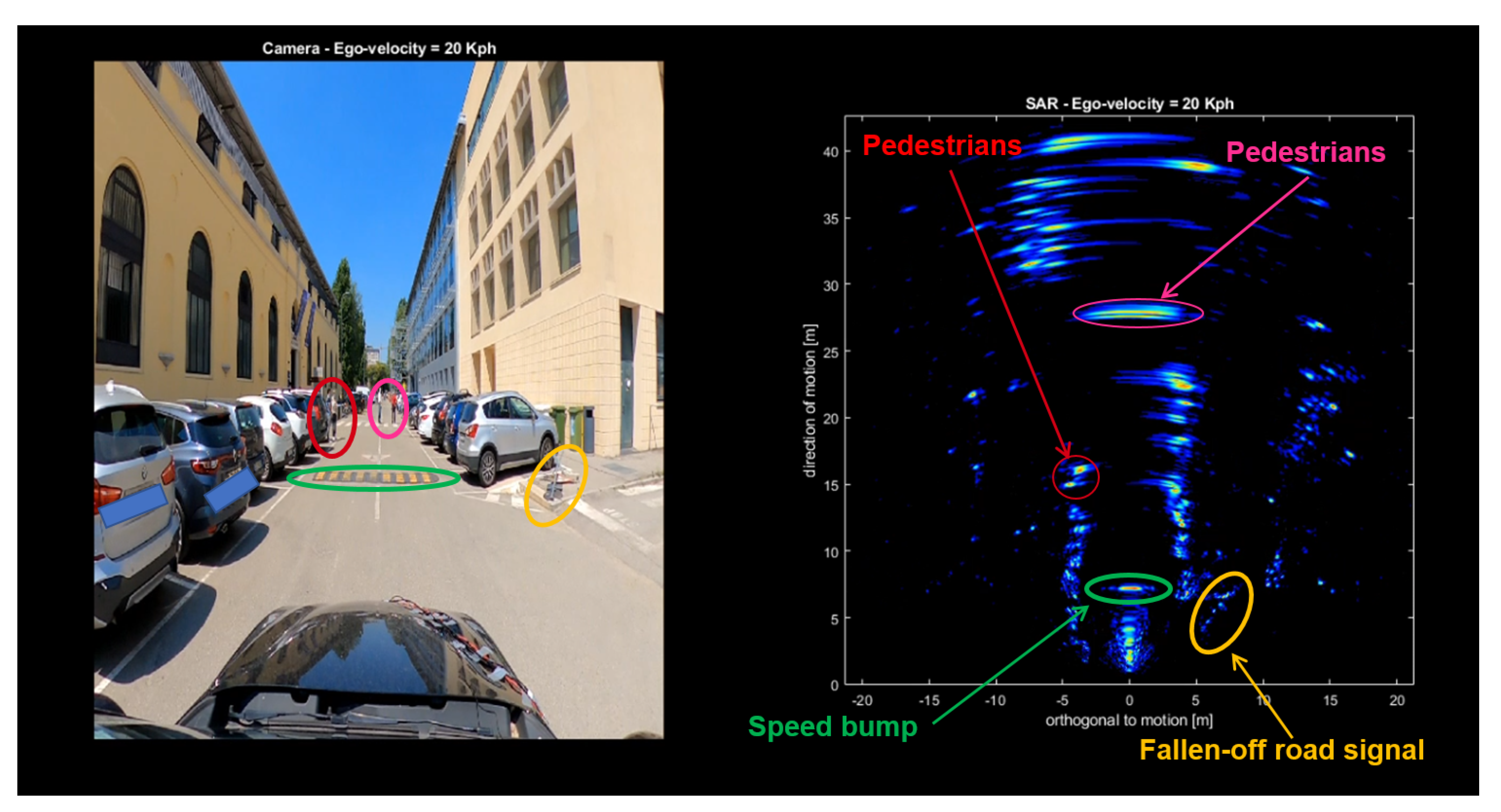
Figure 10 and Figure 11 show two examples of forward-SAR imaging in a closed road and open road, respectively. The radar was working in burst mode, the car was traveling at low speed in an urban and crowded scenario. The aperture exploited is in the order of a few tens of centimeters. Several details can immediately be recognized, including speed bumpers, road signals, parked vehicles, motorbikes, sidewalks, and standing pedestrians.

In commenting those images, it is worth recalling that forward-SAR imaging does not provide resolution right in front of the vehicle, as discussed in Section 3. This is noticeable in Figure 10 where the pedestrians in the purple circle are smeared out in the angular direction. Still, it is sufficient to consider a slightly off-boresight angle to have a considerable resolution improvement compared to standard MIMO radars (see, for example, the pedestrians in the red circle in Figure 10). In the same figure it is also possible to recognize the reflection from the ground in front of the car at very near range. The same kind of reflection can be seen in all the images later on in the paper.

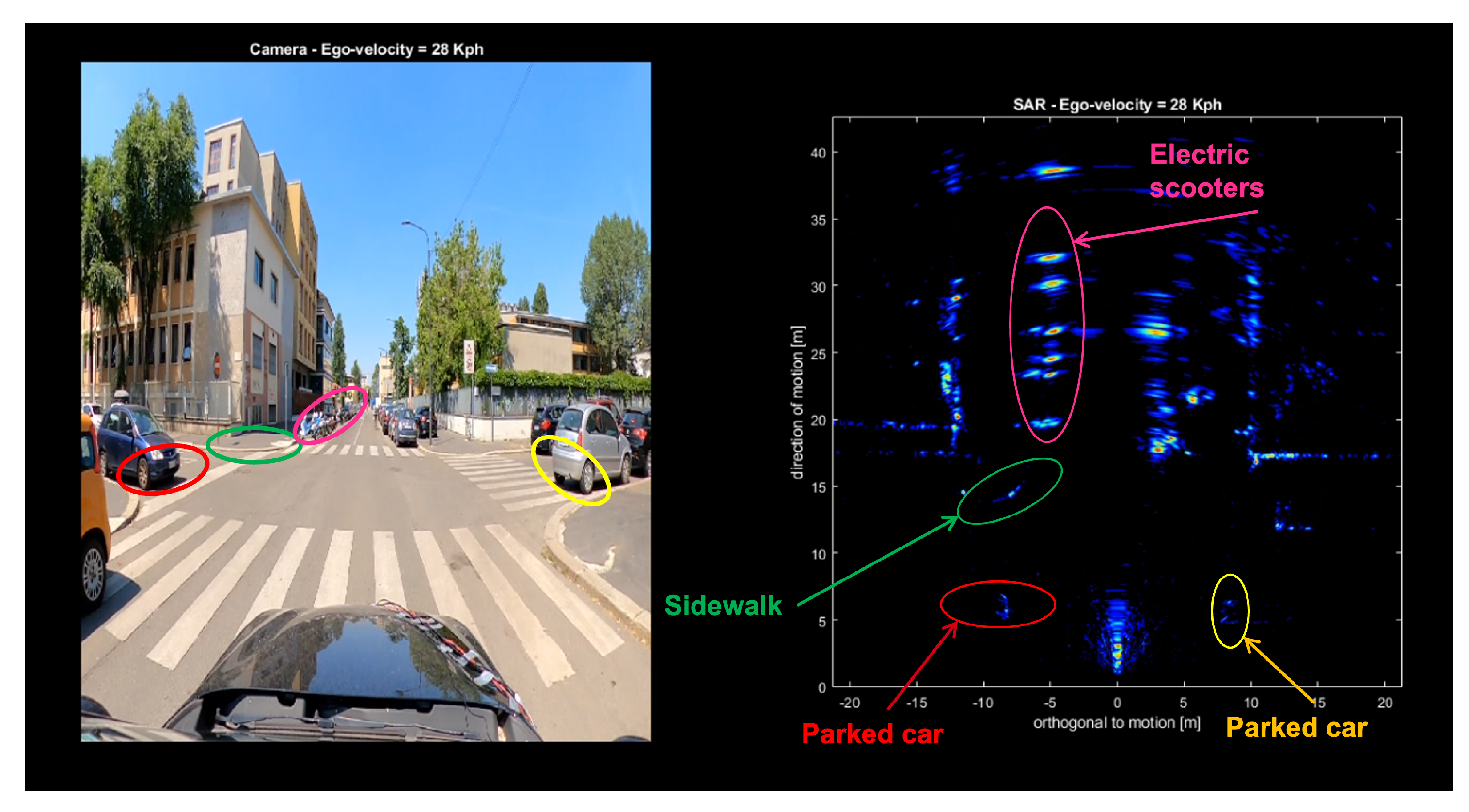
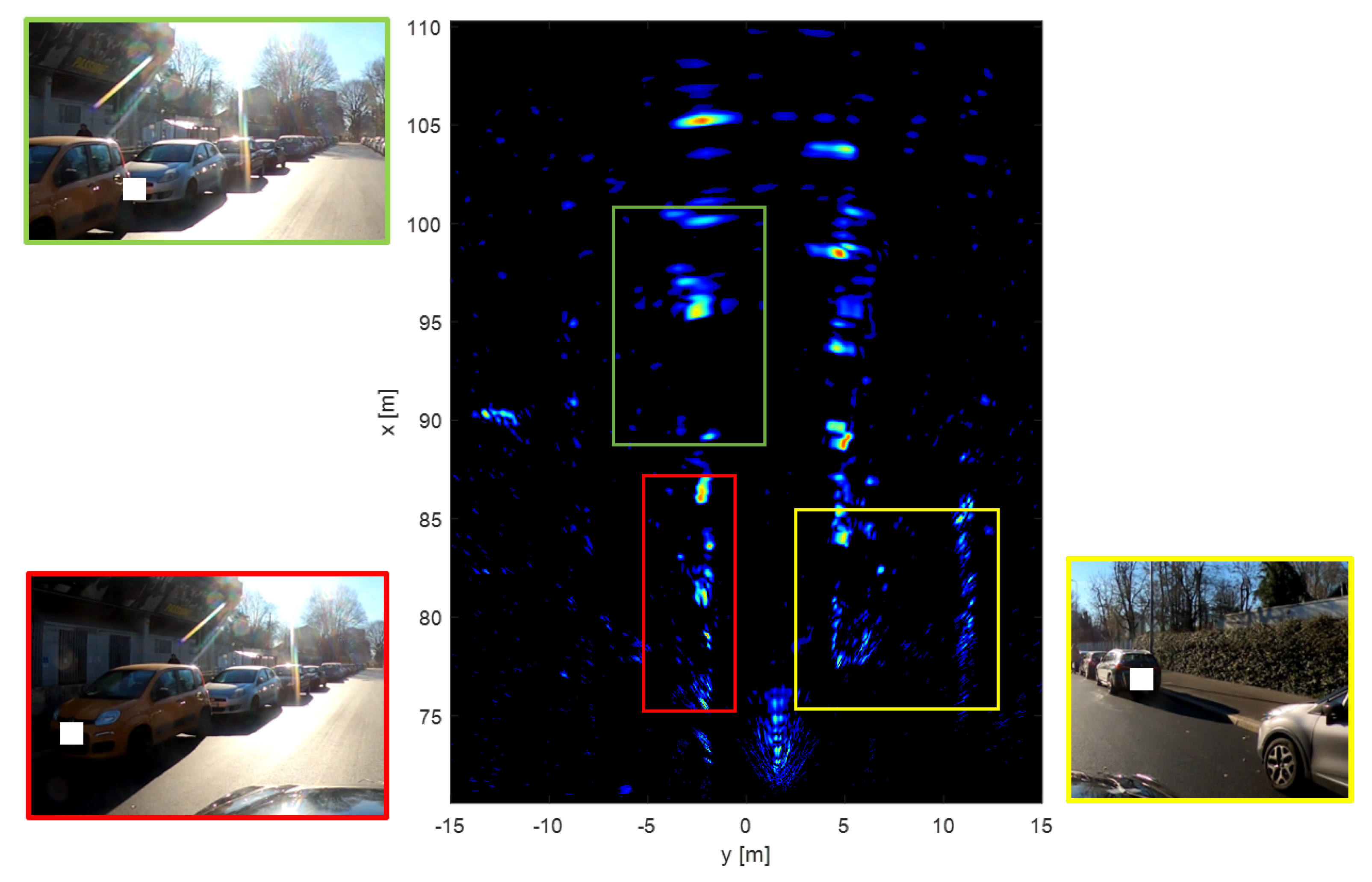
In addition, in Figure 11, several details are recognizable starting from the usual parked cars and sidewalks (yellow, green, and red circles) up to the electric scooters. Interestingly, these targets appear as bright targets in the SAR image, although they are characterized by extended plastic bodies. Another snapshot from a forward-looking acquisition campaign is shown in Figure 12. In the red box, the parked cars on the car’s left are shown. The shapes of these vehicles are distinguishable in the radar image. Again, the resolution is degraded at boresight as easily confirmed by looking in the green box in the radar image. In this region, we have again parked cars, but their details are much less recognizable than those in the red box. We can notice the presence of free parking lots, but the profiles of single cars are less distinguishable. Instead, a free parking slot, parked cars, the sidewalk, and a hedge are depicted in the yellow box.

5.3. Detection of Pedestrians

One of the most challenging scenarios for automotive radars is the detection of pedestrians. Their low radar cross section (RCS) compared to the typical RCS of a vehicle makes them not trivial to detect. Still, pedestrians are among the most vulnerable targets that AD needs to correctly and reliably detect to avoid accidents.

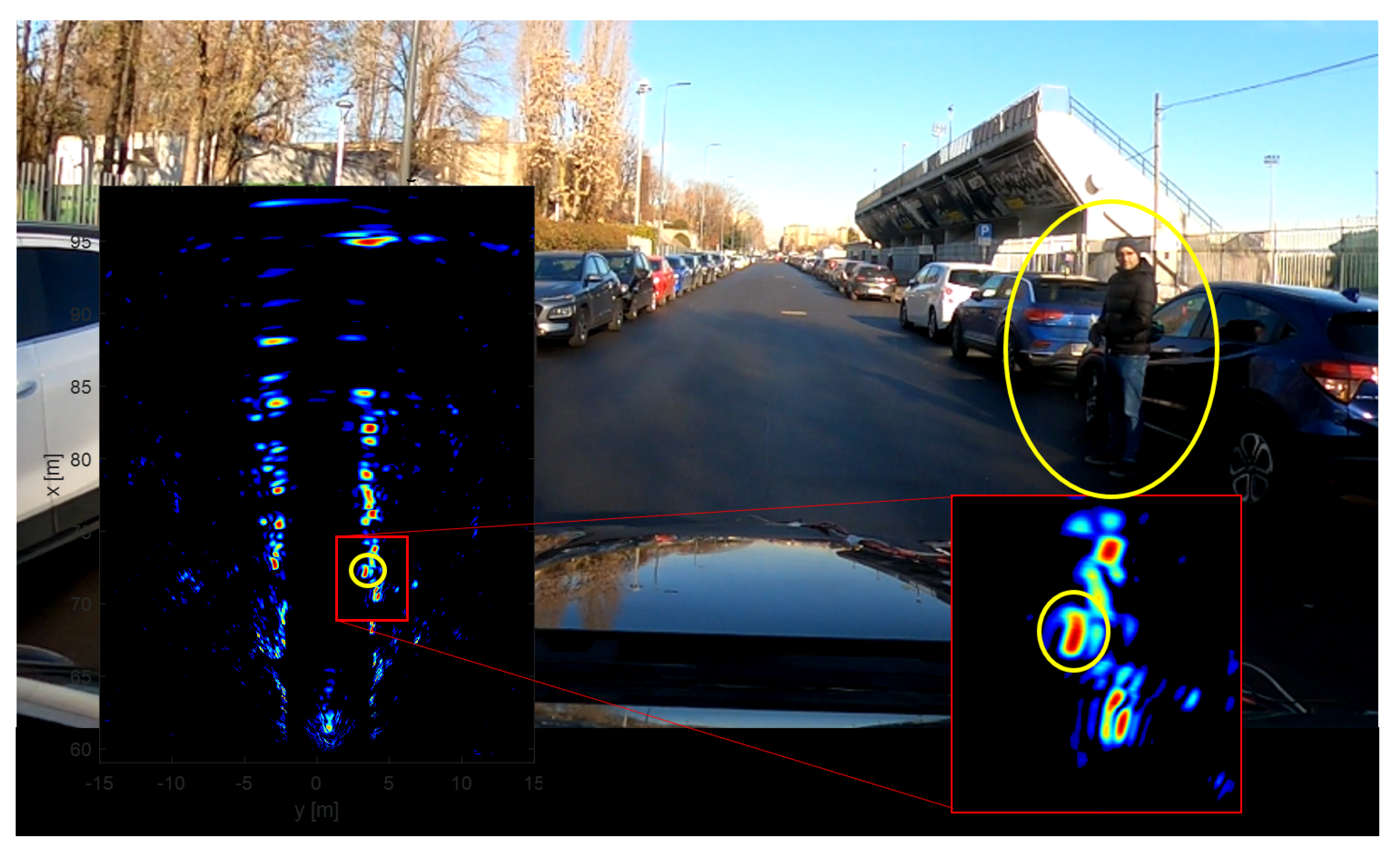
Thanks to the high resolution provided by SAR processing, standing and moving pedestrians are easily spotted. We show herein the capability of SAR to detect pedestrians even in a most critical scenario, such as when a human is standing next to a vehicle having a much bigger RCS. This could represent a safety-critical situation where the pedestrian is waiting before approaching the lane. The detection with a standard MIMO device would be missed with high probability due to insufficient resolution/SNR. This is not the case with SAR, as shown in Figure 13, for which angular resolution is sufficiently fine to clearly distinguish a human body right next to a parked vehicle.

5.4. SAR Imaging of Moving Targets

As explained in Section 4.2, SAR processing requires the knowledge of the phase history of each target along the slow-time to enable the correct imaging [38]. In all previous experiments such phase histories were computed under the assumption that targets are stationary, so that any variation of distance is totally ascribed to the motion of the ego-vehicle. Yet, this choice is not binding in any way, and all it takes to obtain an SAR image of a moving target is to recast the law of motion of the radar sensor in the coordinate frame where the moving target is stationary. In other words, when computing the ranges in the TDBP, we not only use the velocity of the vehicle, but also the velocity of the scene we would like to focus. The result is a formation of a new SAR image for which phase histories are matched to a different law of motion, in which moving targets are focused, whereas stationary targets (as well as all other moving target with a different law of motion) disappear due to defocusing. Of course, an important question concerning imaging of moving targets is how to select the target’s velocities. This could be achieved in principle following a brute force approach consisting in testing all possible velocities within a certain range, though at the cost of a large increase in computational costs. For this work, we followed instead a more simple approach, consisting in running a Doppler analysis of sub-images to derive a preliminary estimation of the velocities of all relevant targets. This information is then used to derive the target’s law of motion, and plugged into the focusing processor. 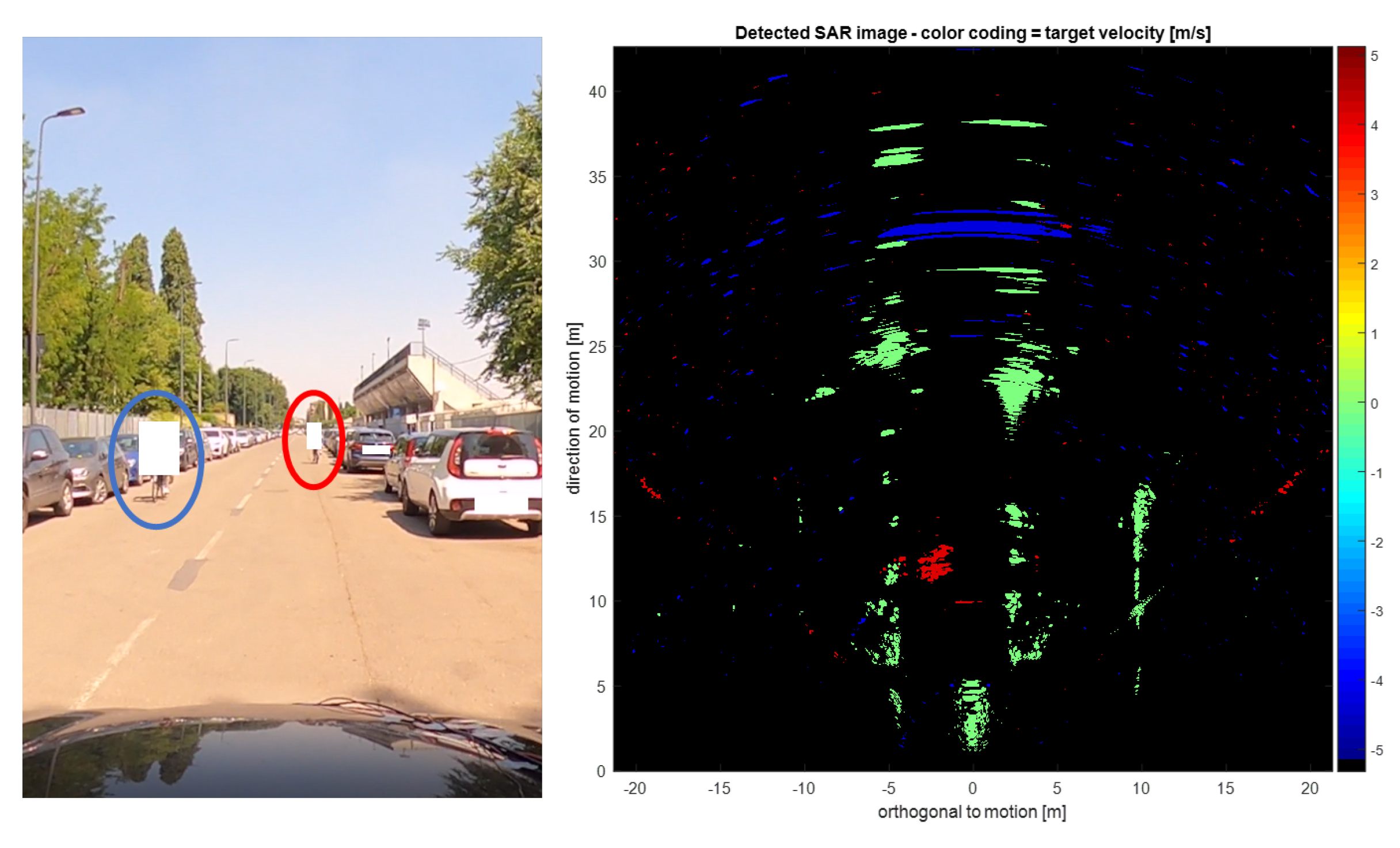A first example of this procedure is shown in Figure 14, which was obtained by assigning a velocity value to all detected targets.

In this case, the green pixels correspond to the static scenario: the usual fences, cars, and free parking lots are distinguishable. The red color corresponds to targets moving towards the experimental vehicle. In particular, we see a cyclist moving at roughly 5 m/s. The same is valid for the cyclist at boresight (in blue), which is moving in the opposite direction. We remark that all the considerations about the angular resolution are still valid for the images of moving targets. This latter cyclist is exactly at boresight, thus where the SAR resolution is poor. 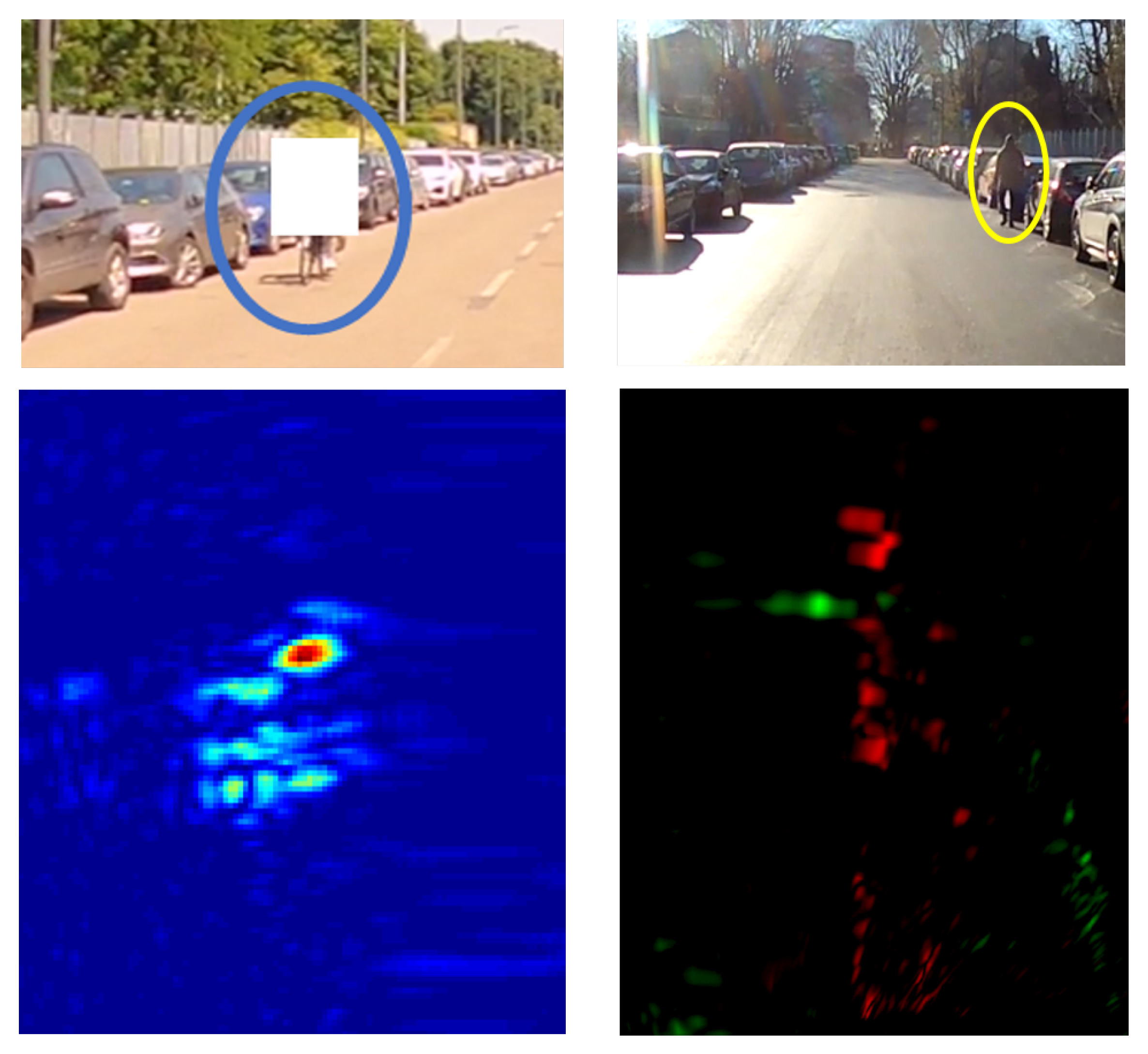In Figure 15 on the left, the same cyclist of Figure 14 is depicted. Here, the bright peak is associated with the dominant Doppler frequency used for the determination of the motion, whereas the areas with less intensity in the vicinity are most likely due to micro-Doppler variations associated with different parts of the bike.

In Figure 15 on the right, a walking pedestrian is depicted. The presence of a walking pedestrian in the roadway is typical in the urban scenario, and thus the system must be able to detect this potentially dangerous situation. In the same figure, the SAR RGB color composite is present. In red we encoded the static scene while in green the targets moving at roughly 1.8 m/s away from the vehicle. Similarly to the case of the moving bicycle, the moving pedestrian is observed to give rise to a dominant peak, used for the determination of motion, surrounded by diffuse contributions associated with micro-Doppler variations.

6. Conclusions

In this paper, we have discussed the application of SAR imaging in the automotive context. The potentials of SAR imaging were analyzed by evaluating the implications of coherent data processing over a significantly longer integration time than allowed by conventional radar imaging. Relevant technological aspects were identified and used to derive a set of basic requirements for the implementation of SAR processing. Finally, an experimental demonstration was provided by showing high resolution SAR images of urban scenarios derived from campaign data acquired with an 8-channel MIMO device.

Physics tells that SAR processing can largely outperform traditional radar imaging for targets that are found at least slightly to the side of the direction of motion of the ego-vehicle. For this reason, it is our opinion that SAR processing constitutes an ideal and natural complement to current automotive radars, and could therefore be systematically used to build an awareness of the whole external environment in which the vehicle moves. In this sense, the concept of automotive SAR processing appears to be mostly suited to the cases of urban or sub-urban scenarios, typically characterized by complex and dynamic environments, rather than for driving on highways. In support of this conclusion, we have provided several experimental demonstrations that SAR imaging can be successfully used to generate high-resolution maps of urban environments, resulting in the possibility to clearly distinguish parked vehicles (not just cars, but also small electric scooters), urban structures (including fences, poles, railings, buildings, and sidewalks), stationary and moving pedestrians, and bicycle riders.

From a technological perspective, it is clear that automotive SAR will have to be implemented on a multichannel device, to guarantee unambiguous imaging using the typical transmission rate of current devices. An important aspect of automotive SAR processing is the estimation of the ego-velocity, as it needs to be known to within an accuracy higher than allowed by low-cost navigational sensors. The work in this paper confirms that such an accuracy is actually achievable if data are acquired with at least a few channels. Still, we deem an open question whether this result could actually be achieved in any kind of weather and road conditions, which calls for extensive experimental campaigns. We deem that SAR focusing algorithms based on the concept of FBP provide the best processing architecture for the automotive case, in that they can handle non-uniform and non-straight motions and allow for a seamless integration of ego-velocity retrieval and multichannel processing. Concerning computational costs, we agree with other research in the literature that any real-time implementation of automotive SAR processing will quite likely require dedicated processing resources, possibly including graphical processing units (GPU). Yet, we remark that the required computing resources are currently compatible to those of modern commercial devices (including smartphones). On this ground, we deem that real-time SAR processing can realistically be made compatible with mass-market production in the immediate future.

It is our opinion that further research should be focused on providing elements to attract future public and private stakeholders towards the concept of automotive SAR imaging. This would require in the first place to run extensive acquisition campaigns under the largest variety of road and meteorological conditions. In doing so, SAR imaging could be thoroughly tested and compared against other types of sensors in scenarios including heavy rain, fog, and dust. In addition to that, we deem that the SAR capability to image the targets at superior spatial resolution and the observed micro-Doppler signature of moving targets might represent new and powerful tools towards improved target recognition.