A Multi-Pulse Cross Ambiguity Function for the Wideband TDOA and FDOA to Locate an Emitter Passively

Abstract

The time difference of arrival (TDOA) and frequency difference of arrival (FDOA) between two receivers are widely used to locate an emitter. Algorithms based on cross ambiguity functions can simultaneously estimate the TDOA and FDOA accurately. However, the algorithms, including the joint processing of received data, require transferring a large volume of data to a central computing unit. It can be a heavy load for the data link, especially for a wideband signal obtained at a high sampling rate. Thus, we proposed a multi-pulse cross ambiguity function (MPCAF) to compress the data before transmitting and then estimate the TDOA and FDOA with the compressed data. The MPCAF consists of two components. First, the raw data are compressed with a proposed two-dimensional compression function. Two methods to construct a reference pulse used in the two-dimensional compression function are considered: a raw data-based method constructs the pulse directly from the received signal, and a signal parameter-based method constructs it through the parameters of the received signal. Second, a wideband cross-correlation function is studied to refine the TDOA and FDOA estimates with the compressed data. The simulation and Cramer–Rao lower bound (CRLB) analyses show that the proposed method dramatically reduces the data transmission load but estimate the TDOA and FDOA well. The hardware-in-the-loop simulation confirms the method’s effectiveness.

1. Introduction

Locating an emitter with passive receivers has been studied [1,2,3,4,5,6] and used in surveillance, navigation, and wireless communications [7,8,9,10]. The array antenna and the direction of arrival [4] are widely used in the localization of emitters. Further studies [11] apply the methods employed in time-reversal imaging [12] to emitter localization or imaging. The traditional methods, such as the MUSIC algorithm and statistical methods, are also applied to emitter imaging [13,14]. With multiple receivers, the time difference of arrival (TDOA) and frequency difference of arrival (FDOA) are critical parameters in the locating algorithms [15,16,17,18,19,20,21,22]. The TDOA and FDOA measured by two moving receivers define two hyperbolas, and their intersection locates an emitter [23,24].

To estimate the TDOA and FDOA, one typically maximizes a cross ambiguity function (CAF) [25]. It is efficient for a narrowband signal. However, the CAF will produce double peaks when dealing with wideband signals [26,27]. The short-time CAF’s coherent summation (CAF-CS) algorithm has also been studied [28]. It calculates multiple CAFs for each short time block, and then the CAFs are coherently combined after compensating for the time and phase difference from the first CAF. The Keystone transform-based method (KTM) is another method to estimate the TDOA and FDOA from wideband pulse signals [29]. The received signals are arranged into a two-dimensional (2-D) matrix, and the transform compensates for the time difference. Then, a Fourier transform is used to achieve a coherent summation of all received signals. The CAF-CS algorithm and KTM improve the estimation accuracy for wideband signals but require transferring data to a central computing unit [30,31]. A comparison of the three methods is listed in

Table 1. Comparison of three methods.

Method	Main Distinctive Characteristics
CAF	Calculating the TDOA and FDOA with the whole raw data.
CAF-CS	Dividing the raw data into multiple segments, calculating the CAF with each segment data, and combining multiple CAFs coherently.
KTM	Arranging the raw data into a 2-D matrix, calculating the TDOA in the range frequency domain via conjugate multiplication, and calculating the FDOA in the azimuth time domain by FFT.

. Unfortunately, the emitter is usually an unknown source, and the sampling rate can be high. Thus, the overall data volume may be too large to be transmitted efficiently. A common solution is to compress the received data. A two-step TDOA and FDOA estimation using the optimal interpolation factor is an example [32]. The factor is set at a low sampling rate as long as the requirement of the Nyquist sampling theorem is met. Unfortunately, the compressed result for a signal with a bandwidth up to GHz can be unsatisfactory.

For the moving sensors, satellites in a group, or unmanned aerial vehicles (UAVs) in a sensor network [33,34], the transmit bandwidth cannot afford such data transmission volume. Thus, a multi-pulse cross ambiguity function (MPCAF) is proposed to reduce the data volume. It consists of two components. First, the data from a receiver is compressed in the range time domain through a reference pulse. As the estimated parameters of the received signal may usually not be available, we propose two methods of constructing the reference pulse. The raw data-based method uses one received pulse as the reference pulse, while the signal parameter-based method constructs the reference pulse using known parameters. Next, the modified Keystone transform is used to correct the range cell migration (RCM). The azimuth Fourier transform compresses the data in the azimuth frequency domain. Then, each receiver’s TOA and Doppler frequency are obtained, and the TOAs and Doppler frequency compute the coarse estimates of the TDOA and FDOA from two receivers. The compressed data are next transmitted to a central computing device. Second, a 2-D wideband cross-correlation function is employed to refine the coarsely estimated TDOA and FDOA. With the proposed MPCAF method, the raw data are significantly compressed, and accurate TDOA and FDOA estimates are obtained.

The paper is organized as follows. Section 2 presents a signal model, and the proposed MPCAF is shown in Section 3. In Section 4, the TDOA and FDOA are estimated and assessed. Simulation results are presented in Section 5. The conclusion is drawn in Section 6.

For reference, a list of all the acronyms, operators, and important matrixes employed in the paper is given as follows

(1)

Acronyms

TDOA	Time Difference of Arrival
FDOA	Frequency Difference of Arrival
UAV	Unmanned Aerial Vehicle
MPCAF	Multi-Pulse Cross Ambiguity Function
CRLB	Cramer–Rao Lower Bound
CAF	Cross Ambiguity Function
CAF-CS	CAF’s Coherent Summation
KTM	Keystone Transform-Based Method
2-D	Two-Dimensional
TOA	Time of Arrival
RCM	Range Cell Migration
PRT	Pulse Repetition Time
PRF	Pulse Repetition Frequency
FFT	Fast Fourier Transform
IFFT	Inverse Fast Fourier Transform
SNR	Signal-to-Noise Ratio
LFM	Linear Frequency Modulation
SAR	Synthetic Aperture Radar

(2)

Operators

*	Conjugate operator
$\otimes$	Convolution operator
T	Transposed operator
$\mathrm{diag}\{·\}$	Diagonal matrix
$\Re \{·\}$	Real part
$\Im \{·\}$	Imaginary part
$\arg \underset{\tau ,v}{\max }(f(\tau ,v))$	Parameter dual (τ,v) that maximizes f(τ,v)

(3)

Matrix

$\tilde{s}$	The transmitted signals in the frequency domain
Ti	TOA matrix of receiver i
F1,m	The m-th Doppler matrix
Hm0	The reference pulse in a raw data-based method
T′m0	TDOA offset matrix
G	The reference pulse in a signal parameter-based method

2. A Signal Model

The geometry of an emitter, P, and two moving receivers (#1 and #2) is shown in Figure 1. The speed of both receivers is v_rec. At the center of a short synthetic aperture, the slant angles of the receivers are θ₁ and θ₂, respectively. At time t, the slant range between Receiver #1 and P is R₁(t), and R₂(t) is the range from Receiver #2 to P. With the slant range model [35], one obtains the slant range of Receiver #1 as

$$R_1(t)\approx R_0-v_{\mathrm{rec}}\cos {\mathsf{\theta }}_1(t-t_{c1})+\frac{v_{\mathrm{rec}}^2{\sin }^2{\mathsf{\theta }}_1}{2R_0}{(t-t_{c1})}^2$$

(1)

where tc₁ is the center time, and R₀ is the range at t_c1.

The short synthetic aperture assumption satisfies

$$\frac{v_{\mathrm{rec}}^2{\sin }^2{\mathsf{\theta }}_1}{\lambda R_0}{T}_{\max }^2\pi <\frac{\pi }{8}$$

(2)

where λ is the wavelength of the emitter’s central frequency, f_c. T_max is the maximum time length of an aperture. Then, the time limit of a short synthetic aperture is

$$T_{\max }<\frac{1}{2v_{\mathrm{rec}}\sin {\mathsf{\theta }}_1}\sqrt{\frac{\lambda R_0}{2}}$$

(3)

If the time duration of the received data satisfies (3), the assumption of the short synthetic aperture is accepted, and the quadratic item in (1) can be ignored. Thus, R₁(t) is a linear function of t. (Similarly, R₂(t) is a linear function of t under the condition of a short synthetic aperture).

Let the pulse repetition time (PRT) of a received signal be T. Then, the time offset of the m-th pulse is v_recmTcos θ₁/c, where c is the speed of light. Considering the Doppler frequency, f_d = v_recf_ccos θ₁/c, one can express the time offset of the m-th pulse as mTf_d/f_c. Defining the Doppler factor as α₁ = −f_d/f_c, one obtains the azimuth time, t_m = mT. Then, the time offset can be expressed as –α₁t_m. With the assumption that a signal transmitted by an emitter is s(t)exp(j2πf_ct), the m-th pulse received by Receiver #1 is

$$s_1(t_r,t_m)=s(t_r-t_1-{\alpha }_1{t}_m)e^{-j2\pi f_c(t_1+{\alpha }_1{t}_m)}$$

(4)

where t_r is the range time [36,37], and t₁ is the time of arrival (TOA) of Receiver #1. The signal received by Receiver #2 is similar to (4), except that the Doppler factor and TOA differ.

The conventional CAF algorithm uses the signals from both receivers directly and the TDOA and FDOA are obtained by correlation and FFT, respectively. The direct use of raw data requires the transmission of a large amount of data. However, the transmission bandwidth of the satellite platform is limited. Therefore, to alleviate the pressure of data transmission, we propose a multi-pulse CAF that pre-compresses the raw data and then calculate the TDOA and FDOA with the compressed data.

3. Method

In this section, we define the MPCAF with the 2-D data given in the above section and prove the equivalence of the MPCAF computed from the compressed data and the MPCAF obtained from the raw data. Then, the MPCAF is used to estimate the TDOA and FDOA.

3.1. A Multi-Pulse CAF

Definition 1.

An MPCAF is defined as

$$C(\tau ,v)={\displaystyle {\int }_0^T{\displaystyle {\int }_0^{MT}{s}_1(t_r,t_m)s_2^{*}(t_r+\tau ,t_m)e^{-j2\pi v{t}_m}d{t}_m}{e}^{-j2\pi v{t}_r}d{t}_r}$$

(5)

where τ is time, and v is frequency.

The original CAF for the multi-pulse signal can be written in the form of a multi-segment (M) integration or

$$A(\tau ,v)={\displaystyle \sum _{m=0}^M{\displaystyle {\int }_{mT}^{(m+1)T}{s}_1(t)s_2^{*}(t+\tau )e^{-j2\pi vt}dt}}$$

(6)

Changing the upper and lower bounds of the integration, one obtains

$$A(\tau ,v)={\displaystyle \sum _{m=0}^M{\displaystyle {\int }_0^T{s}_1(t-mT)s_2^{*}(t-mT+\tau )e^{-j2\pi v(t-mT)}dt}}$$

(7)

Considering a 2-D signal defined by (4), s₁ (for Receiver #1) and s₂ (for Receiver #2) can be written as s₁(t, t_m) and s₂(t, t_m), respectively. Then (7) is simplified as

$$A(\tau ,v)={\displaystyle \sum _{m=0}^M{\displaystyle {\int }_0^T{s}_1(t_r,t_m)s_2^{*}(t_r+\tau ,t_m)e^{-j2\pi v{t}_r}{e}^{j2\pi v{t}_m}d{t}_r}}$$

(8)

Since $e^{j2\pi v{t}_m}$ is independent of t_r, one can rewrite (8) as

$$A(\tau ,v)={\displaystyle \sum _{m=0}^M{s}_m(\tau ,v)e^{j2\pi v{t}_m}}$$

(9)

with

$$s_m(\tau ,v)={\displaystyle {\int }_0^T{s}_1(t_r,t_m)s_2^{*}(t_r+\tau ,t_m)e^{-j2\pi v{t}_r}d{t}_r}$$

(10)

Equation (10) is the traditional CAF [25] and (9) is the CAF-CS algorithm. Equation (9) shows that the phase difference between the multi-CAFs is 2πvt_m, and it needs to be compensated for the coherent summation. The results of MPCAF and CAF-CS are the same in the τ-v space. However, the CAF-CS algorithm calculates multiple CAF and realizes the summation of multiple 2-D planes. The processing of CAF-CS is in 3-dimensional (3-D) space. The MPCAF divides the raw data into many short pulses, then arranges the short pluses into a 2-D matrix. Indeed, the MPCAF is a 2-D FFT on the cross-correlation matrix. This is the main difference between the MPCAF and CAF-CS.

When the raw data is a pulsed radar signal, the data of each receiver can be compressed separately by constructing a reference function.

Definition 2.

A 2-D compression function for a wideband signal is defined as

$$\begin{gathered} d_1(t,u)={\displaystyle {\int }_0^{MT}[s_1(t,t_m)\otimes h^{*}(t)]e^{-j2\pi u{t}_m}d{t}_m} \\ {d}_2(t,u)={\displaystyle {\int }_0^{MT}[s_2^{*}(t,t_m)\otimes h(t)]e^{-j2\pi u{t}_m}d{t}_m} \end{gathered}$$

(11)

where$\otimes$is a convolution operator, h(t) is the reference pulse for the data compression, and u is the frequency.

Definition 3.

A wideband cross-correlation function based on the compressed data is defined as

$$C^{\prime }(\tau ,v)={\displaystyle {\int }_u{\displaystyle {\int }_t{d}_1(t+\tau ,u)d_2(t,v-u)e^{-j2\pi vt}dtdu}}$$

(12)

For a wideband signal, the signal bandwidth is much wider than the Doppler frequency, thus

$$C^{\prime }(\tau ,v)\approx C(\tau ,v)$$

(13)

The proof of (13) is given in Appendix A.

The problem of large data volume and limited transmission bandwidth can be solved by (13). However, the compression method of wideband signals in (11) is signal-type dependent. Fortunately, signals with bandwidths over 100 MHz are usually used for detection in a radar system. Since the signals are usually periodic and repetitive, the received signal can be compressed by a reference signal. The next section will give the compression method for the wideband signals in a radar system and use the MPCAF to obtain the TODA and FDOA.

3.2. Wideband TDOA and FDOA Estimation Using the MPCAF

As shown in Figure 2, the overall processing flow consists of two main parts, the compression of the received data and the two-step TDOA and FDOA estimations. The data compression includes the range and azimuth compressions. The estimation of the TDOA and FDOA includes a coarse estimation and then a fine estimation. The TOAs and Doppler frequencies of the compressed data give the coarse estimation, and the compressed data complete the fine one.

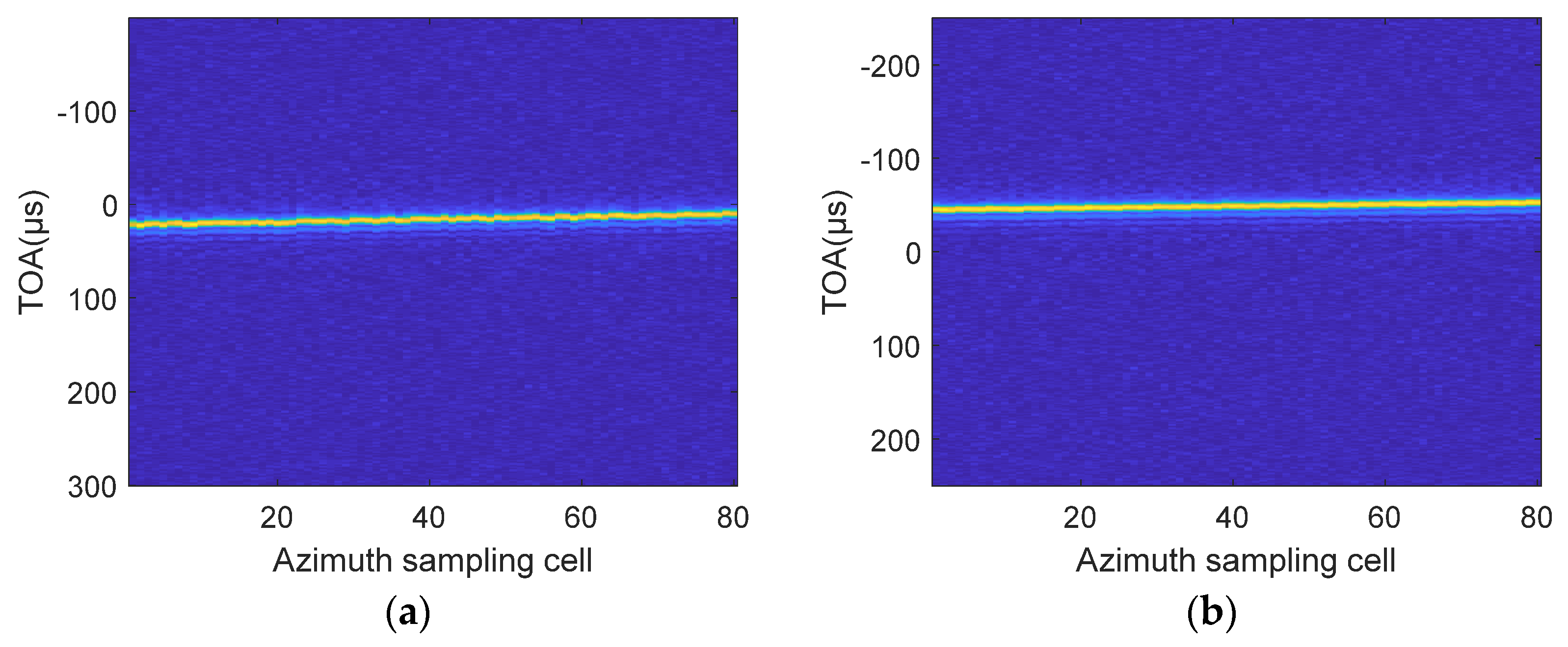
3.2.1. Data Compression and Coarse TDOA and FDOA Estimations

A common solution for compressing a periodic and repetitive signal is to construct a reference signal and perform a matched filtering. The reference pulse is constructed in the frequency domain to avoid the time-intensive convolution operation. Thus, the Fourier transform is performed for a received signal, and then the reference pulse is constructed. A general form of a wideband signal in the frequency domain is

$$s_1(f,mT)=s(f)e^{-j2\pi (f_c+f)t_1}{e}^{-j2\pi (f_c+f){\alpha }_1{t}_m}$$

(14)

where s(f) is the Fourier transform of the baseband signal and f is baseband frequency. One can denote the baseband frequency by a vector of

$$f={[f_0,f_1,\cdots ,f_{N-1}]}^{\mathrm{T}}$$

(15)

where f_n = nF_s/N with N being the sampling number in the range.

Define

$$\begin{gathered} \tilde{s}=s(f) \\ {T}_1={\mathrm{diag}\{\mathrm{e}}^{-j2\pi f_r{t}_1}\} \\ {F}_{1,m}={\mathrm{diag}\{\mathrm{e}}^{-j2\pi f_r{\alpha }_1{t}_m}\} \end{gathered}$$

(16)

where f_r = f + f_c. Then, the m-th received pulse of Receiver #1 in the range frequency domain is

$$s_{1,m}=T_1{F}_{1,m}\tilde{s}$$

(17)

Define s_i as a 2-D signal matrix, which contains M pulses

$$\begin{gathered} s_1=[s_{1,0},s_{1,1},\cdots ,s_{1,M-1}] \\ {s}_2=[s_{2,0},s_{2,1},\cdots ,s_{2,M-1}] \end{gathered}$$

(18)

As the sampling rate related to the signal bandwidth is often set to GHz, a massive volume of data is collected and transmitted to a central computing unit, burdening the data transmission system. We propose a data compression method in the range-Doppler domain to reduce the burden. The main idea is to compensate for the modulation phase of the received signal. The Doppler frequency affects the phase in the azimuth domain, and the baseband signal modulates the phase in the range domain. The former is compensated with the azimuth FFT. A reference pulse is usually used to compensate for the latter. A straightforward way to construct a reference pulse is to use a received signal as the reference directly. The approach does not require estimating the signal parameters, simplifying the equipment requirement and processing flow. Another way is to construct the reference pulse with the parameters of the received signal. In this case, the reference is noiseless, and the estimation is better in a low SNR scenario. Depending on the device capability, SNR, and accuracy requirement, one can construct the reference either way flexibly. With the two methods of constructing a reference pulse, we propose two algorithms for data compression.

Method A: A raw data-based method

For an unknown LFM signal, the reference pulse can be constructed by the m₀-th pulse received from a selected receiver with a high SNR. With Receiver #1 as an example, the reference pulse is the m₀-th pulse in s₁, expressed as

$$H_{m_0}=s_{1,0}^{*}=T_1^{*}{\phi }^{*}(f_r)\mathrm{diag}\{{\tilde{s}}^{*}\}$$

(19)

where ^* is a conjugate operator and $\phi (f_r)={\mathrm{diag}\{\mathrm{e}}^{-j2\pi f_r{\alpha }_1{t}_m}\}$. m₀ can be selected at any azimuth time. Usually, the synthetic aperture center time m₀ = 0 is selected. Indeed, the reference pulse contains the TOA term and the Doppler frequency term. After the data compression, the signal matrix of Receiver #1 is

$$H_{m_0}{s}_1=\phi (f_r)[F_{1,0}{\tilde{s}}^2,F_{1,1}{\tilde{s}}^2,\cdots ,F_{1,M-1}{\tilde{s}}^2]$$

(20)

where ${\tilde{s}}^2$ = $\mathrm{diag}\left\{{\tilde{s}}^{*}\right\}\tilde{s}$ is the amplitude of the compressed signal in the range frequency domain. F_1,m represents the Doppler frequency and is a coupling of range frequency and azimuth time. The coupling causes the TOA to be time-varying in azimuth, which is equivalent to the RCM in SAR imaging.

In (20), the data after compression do not contain the TOA information. Instead, the information is included in the reference pulse. After compressing the data from the other receiver by the reference pulse, one obtains

$$H_{m_0}{s}_2=T_1^{*}{T}_2{T}_{m_0}^{\prime }{\phi }^{*}(f_r)[F_{2,0}{\tilde{s}}^2,\cdots ,F_{2,M-1}{\tilde{s}}^2]$$

(21)

where $T_{m_0}^{\prime }$ = ${\mathrm{diag}\{\mathrm{e}}^{-j2\pi f_r({\alpha }_2-{\alpha }_1)t_{m_0}}\}$. As the TOA of each receiver is time-varying during the movement of the receivers, the TDOA is also time-varying. $T_{m_0}^{\prime }$ represents the TDOA offset from the zero time. Figure 3a shows that one can obtain the TODA at the central time by setting t_m0 = 0. Figure 3b shows that if the parameter t_m0 in the reference pulse is not zero, the compressed result is shifted by time α₁t_m0 relative to Figure 3a. At t_m0, the offset of the TDOA is (α₂ − α₁)t_m0. Thus, the TDOA at different times can be obtained by selecting reference pulses at different times.

The next step is to compress the data in azimuth. The coupling of the range frequency and azimuth causes the RCM and the Doppler frequency to vary with range frequency. The RCM makes a signal distributed in multiple range time and azimuth frequency sampling units, affecting the azimuth compression. Thus, the decoupling is crucial to compress the signal in the azimuth domain. The Keystone transform [38] is usually used for the decoupling, and the TDOA at the central moment can be obtained. However, the TDOA varies with azimuth times, and a reference pulse can be selected at any azimuth time. As the pulse usually corresponds to the receiver position used in a locating algorithm, it is necessary to obtain the TDOA at the azimuth time of the reference pulse. Thus, a modified Keystone transformation is used to estimate the TDOA at any azimuth time. The modified transformation is

$$t_m^{\prime }=\frac{f_r}{f_c}(t_m-t_{m_0})+t_{m_0}$$

(22)

In the modification, the original azimuth time, t_m, is replaced by a new azimuth time, t′_m. The frequency-dependent phase ${\mathrm{e}}^{-j2\pi f_r{\alpha }_1(t_m-t_{m_0})}$ is replaced by a frequency-independent phase ${\mathrm{e}}^{-j2\pi f_c{\alpha }_1(t_m^{\prime }-t_{m_0})}$, eliminating the coupling. After the transformation, one obtains

$${\phi }^{*}(f_r)F_{1,m}=e^{j2\pi f_c{\alpha }_1{t}_{m_0}}{e}^{-j2\pi f_c{\alpha }_1{t}_m^{\prime }}I$$

(23)

and

$$H_{m_0}{s}_1={\phi }_1[{\tilde{s}}^2,{\tilde{s}}^2,\cdots ,{\tilde{s}}^2]F_{\mathrm{MA}1}$$

(24)

where $F_{\mathrm{MA}1}={\mathrm{diag}\{\mathrm{e}}^{-j2\pi f_c{\alpha }_1{t}_{\mathrm{MA}1}}\}$, with $t_{\mathrm{MA}1}=[t_0^{\prime },\cdots t_{M-1}^{\prime }]$ being the new azimuth time. ${\phi }_1=e^{j2\pi f_c{\alpha }_1{t}_{m_0}}$ is a constant phase. After the range IFFT and azimuth FFT, the peak of the compressed data appears at time t = 0 and Doppler frequency v = α₁f_c.

Method B: A signal parameter-based method

Once a signal’s parameters are known, the reference pulse can be constructed with the known parameters. For an LFM signal, s(f) can be written as

$$s(f)=\mathrm{rect}(\frac{f}{B}{)\mathrm{e}}^{j\pi f^2/\gamma }$$

(25)

where B is the signal bandwidth, and γ is the chirp rate. Let us define

$$f^2={[f_0^2,f_1^2,\cdots ,f_{N-1}^2]}^{\mathrm{T}}$$

(26)

The reference pulse can be constructed as

$$G={\mathrm{diag}\{\mathrm{e}}^{-j\pi f^2/\gamma }\}$$

(27)

and is obtained after the range compression

$$G{s}_1=T_1[F_{1,0}\tilde{s},F_{1,1}\tilde{s},\cdots ,F_{1,M-1}\tilde{s}]$$

(28)

Different from the former method, (28) maintains the TOA of each receiver, which means the true TOA of each receiver can be obtained. Equation (28) also suffers a coupling of range frequency and azimuth time. To handle the coupling, we use the modified Keystone transformation and set t_m0 = 0. Then, phase ${\mathrm{e}}^{-j2\pi f_r{\alpha }_1{t}_m}$ is replaced with ${\mathrm{e}}^{-j2\pi f_c{\alpha }_1{t}_m^{″}}$. After the transformation, one obtains

$$F_{1,m}=e^{-j2\pi f_c{\alpha }_1{t}_m^{″}}I$$

(29)

and (28) becomes

$$G{s}_1=T_1[\tilde{s},\tilde{s},\cdots ,\tilde{s}]F_{\mathrm{MB}1}$$

(30)

where $F_{\mathrm{MB}1}={\mathrm{diag}\{\mathrm{e}}^{-j2\pi f_c{\alpha }_1{t}_{\mathrm{MB}1}}\}$, with $t_{\mathrm{MB}1}=[t_0^{″},\cdots t_{M-1}^{″}]$ being another new azimuth time. After the range IFT, the peak appears at t = t₁ and v = α₁ f_c.

The well-compressed data should have little energy inside the side lobes, and one can only transmit the data in the main lobe. However, the data cannot be entirely and well compressed due to possible parameter errors in the reference pulse. In this case, sending more data can better estimate the TDOA and FDOA in the second step. The data within the first side lobes are generally transmitted.

3.2.2. Refining TDOA and FDOA Estimations

After the data compression, the data are concentrated into a small area in the range-Doppler plane. Detecting the peak of the compressed data, one obtains the TOA and Doppler frequency of each receiver. Assuming that the TOA of the two receivers is t₁ and t₂, respectively, and the corresponding Doppler is v₁ and v₂. The coarse TDOA and FDOA estimates are

$$\begin{gathered} {\tau }_{\mathrm{coarse}}=t_1-t_2 \\ {v}_{\mathrm{coarse}}=v_1-v_2 \end{gathered}$$

(31)

Ideally, the transmitted data are centered at the true TOA and Doppler frequency lo-cation. Unfortunately, noise causes errors in the coarse TDOA and FDOA estimations and the center of the transmitted data is offset. Thus, joint processing is needed to refine the estimation. As the compressed data is small in volume, the TDOA and FDOA can be calculated by a wideband cross-correlation function proposed in Section 3, avoiding the data reconstruction in a CAF-based algorithm. The estimated TDOA and FDOA using the function is

$$C_2(\tau ,v)={\displaystyle {\int }_u{\displaystyle {\int }_t{r}_1(t+\tau ,u)r_2(t,v-u)e^{-j2\pi vt}dtdu}}$$

(32)

where r₁ and r₂ are compressed data from the two receivers. Then, the TDOA and FDOA estimations in the second step are

$$({\tau }^{\prime },{\upsilon }^{\prime })=\arg \underset{\tau ,v}{\max }(C_2(\tau ,v))$$

(33)

and the refined TDOA and FDOA are

$$\begin{gathered} {\tau }_{\mathrm{refined}}={\tau }_{\mathrm{coarse}}+{\tau }^{\prime } \\ {v}_{\mathrm{refined}}=v_{\mathrm{coarse}}+v^{\prime } \end{gathered}$$

(34)

Figure 4 illustrates the refining TDOA and FDOA estimations. The transmitted data with the true TOA and Doppler frequency is shown on the left in the figure. The data with offset TOA and Doppler frequency is shown on the right of the figure. The joint processing aligns the true TOA and Doppler frequency in the transmitted data, refining the TDOA and FDOA estimations.

4. Performance Analysis and Consideration in Applications

4.1. CRLB Analysis

The received signal with noise w_i,m is

$$\begin{gathered} r_{1,m}=s_{1,m}+w_{1,m} \\ {r}_{2,m}=s_{2,m}+w_{2,m} \end{gathered}$$

(35)

with

$$\begin{gathered} r_i={[r_{i,0}^{\mathrm{T}},r_{i,1}^{\mathrm{T}},\cdots ,r_{i,M-1}^{\mathrm{T}}]}^{\mathrm{T}} \\ {R}_i=\mathrm{diag}(T_{i,0},T_{i,1},\cdots ,T_{i,M-1}) \\ {A}_i=\mathrm{diag}(F_{i,0},F_{i,1},\cdots ,F_{i,M-1}) \\ S={[{\tilde{s}}^{\mathrm{T}},{\tilde{s}}^{\mathrm{T}},\cdots ,{\tilde{s}}^{\mathrm{T}}]}^{\mathrm{T}} \\ {w}_i={[w_{i,0}^{\mathrm{T}},w_{i,1}^{\mathrm{T}},\cdots ,w_{i,M-1}^{\mathrm{T}}]}^{\mathrm{T}} \end{gathered}$$

(36)

Received signals of the two receivers can be written as

$$\begin{gathered} r_1=R_1{A}_{1}S+w_1 \\ {r}_2=R_2{A}_{2}S+w_2 \end{gathered}$$

(37)

The maximum likelihood estimation obtains the parameter pair θ = [τ₀,v₀]^T from the observation matrix $r=[r_1^{\mathrm{T}},r_2^{\mathrm{T}}{]}^{\mathrm{T}}$. The Cramer–Rao lower bound (CRLB) is

$$J({\mathsf{\theta }}^{\mathrm{T}})=\frac{1}{{\sigma }^2}\Re \left\{D^{\mathrm{H}}D\right\}$$

(38)

where

$$D=\left[D_{\tau }Q{\tilde{r}}_1,D_{\upsilon }Q\tilde{r}\right]$$

(39)

with

$$\begin{gathered} Q=\left[\begin{array}{l}{R}_1{A}_1\\ R_2{A}_2\end{array}\right] \\ {D}_{\tau }=\mathrm{diag}(D_{\tau ,0},D_{\tau ,1},\cdots ,D_{\tau ,M-1}) \\ {D}_{\upsilon }=\mathrm{diag}(D_{\upsilon ,0},D_{\upsilon ,1},\cdots ,D_{\upsilon ,M-1}) \\ {D}_{\tau ,m}=\mathrm{diag}(-j2\pi f_{r,0},\cdots ,-j2\pi f_{r,N-1}) \\ {D}_{\upsilon ,m}=\mathrm{diag}(-j2\pi \frac{m{f}_{r,0}}{f_{c}PRF},\cdots ,-j2\pi \frac{m{f}_{r,N-1}}{f_{c}PRF}) \end{gathered}$$

(40)

The derivation is detailed in Appendix B.

4.2. Relationship with Cyclostationarity-Based Algorithms

Assumed that two signals used for calculation are

$$\begin{gathered} x(t)=As(t) \\ y(t)=As(t-D)e^{j2\pi f_{d}t} \end{gathered}$$

(41)

A cyclic cross ambiguity function for joint TDOA and FDOA estimation is defined as

$$C_{yx}^{\epsilon }(\tau ,f)={\displaystyle \int R_{yx}^{\epsilon -f}(u){\left(R_{xx}^{\epsilon }(u-\tau )\right)}^{*}{e}^{j\pi fu}du}$$

(42)

where

$$\begin{gathered} R_{xx}^{\epsilon }(\tau )=\frac{1}{T}{\displaystyle {\int }_{-T/2}^{T/2}x(t+\tau /2)x^{*}(t-\tau /2)e^{-j2\pi \epsilon t}dt} \\ {R}_{yx}^{\epsilon }(\tau )=\frac{1}{T}{\displaystyle {\int }_{-T/2}^{T/2}y(t+\tau /2)x^{*}(t-\tau /2)e^{-j2\pi \epsilon t}dt} \end{gathered}$$

(43)

Let

$$f_R(u,f)=R_{xy}^{\epsilon -f}(u){\left(R_{xx}^{\epsilon }(u-\tau )\right)}^{*}{e}^{j\pi fu}$$

(44)

When u = τ and ε = 0, one has

$$\begin{array}{ll}{R}_{xx}^{\epsilon }(0)& =A\frac{1}{T}{\displaystyle {\int }_{-T/2}^{T/2}s(t+\tau /2)s^{*}(t-\tau /2)dt}\\ & =A{R}_{ss}^0(0)\end{array}$$

(45)

and

$$R_{xy}^{-f}(\tau )=\frac{1}{T}{\displaystyle {\int }_{-T/2}^{T/2}x(t-\tau /2)y^{*}(t+\tau /2)e^{j2\pi ft}dt}$$

(46)

Since $R_{ss}^0(0)$ is a real-type number not related to the time delay and Doppler frequency, one obtains

$$\begin{array}{l}{f}_R(\tau ,f)=A^2{R}_{ss}^0(0)R_{ss}^{f_d-f}(\tau -D)e^{-j\pi (f_d-f)D}\\ =A^2{R}_{ss}^0(0)e^{j\pi f_d\tau }{R}_{yx}^{-f}(\tau )\end{array}$$

(47)

The CAF can be expressed as

$$\begin{array}{l}C(\tau ,f)={\displaystyle {\int }_{-T/2}^{T/2}x(t-\tau /2)y^{*}(t+\tau /2)e^{-j2\pi ft}dt}\\ ={\left[{\displaystyle {\int }_{-T/2}^{T/2}y(t+\tau /2)x^{*}(t-\tau /2)e^{j2\pi ft}dt}\right]}^{*}\\ =T{R}_{yx}^{-f}(\tau )\end{array}$$

(48)

The results of (47) and (48) show that the CAF algorithm is a special situation when the cyclic frequency α = 0 and u = τ. As the MP-CAF is proved to be equal to CAF (in Section 3.1), the proposed function is also a special situation in cyclostationarity-based algorithms.

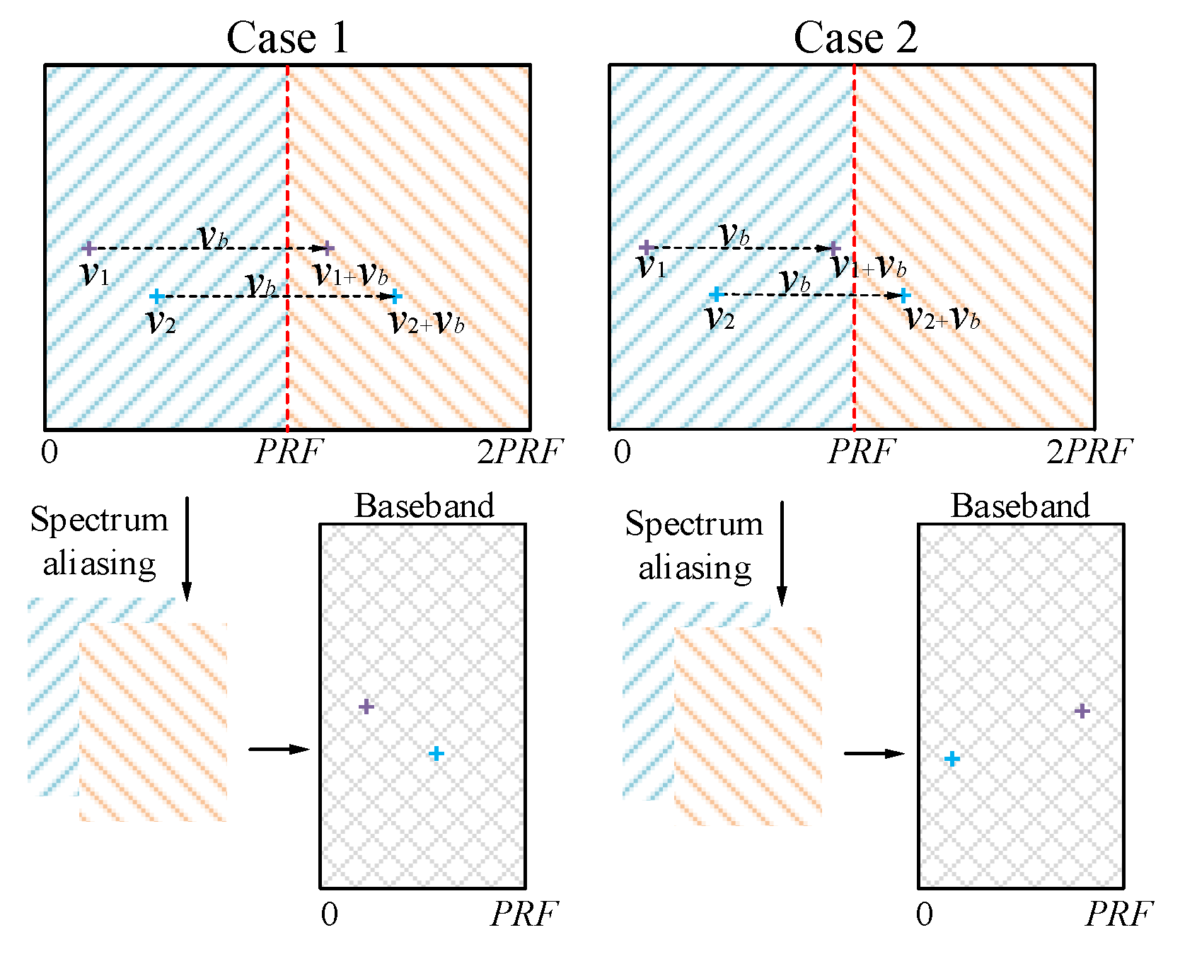
4.3. Doppler Aliasing

According to the signal model proposed in Section 2, Doppler frequency f_cαt_m is related to the azimuth sampling interval T′. The azimuth sampling rate is essential and should equal the pulse repetition frequency (PRF) of the emitter. The mismatch of the two parameters will scale the real azimuth time, causing an additional Doppler frequency of a received signal. Here, the mismatch and its influence are analyzed.

Assuming that the sampling interval is 1/F_s and the mismatch is k sampling units, the additional Doppler frequency is

$$v_e=k{f}_{c}PRF/F_s=nPRF+v_b$$

(49)

where n is the Doppler aliasing number, and v_b is the baseband of the Doppler frequency. The Doppler frequency estimation of Receiver #i (i = 1, 2), ${\widehat{v}}_i$ with v_e is

$${\widehat{v}}_i=nPRF+v_b+v_i$$

(50)

where v_i is the Doppler frequency of the i-th receiver. If v_b = 0, the additional Doppler frequency is an integer multiplied by the PRF. It does not affect the Doppler frequency estimation. In general, v_b is not equal to 0 and has different effects on the baseband of the Doppler frequency. Two cases exist and are discussed.

Case 1: (v_b + v₁) and (v_b + v₂) are larger or smaller than one PRF. The PRF aliasing numbers of the two receivers are the same, and the correct FDOA can be obtained as shown in Case 1, Figure 5. The relative difference in the Doppler frequency has not changed after aliasing.

Case 2: One of (v_b + v₁) and (v_b + v₂) is higher than one PRF. The PRF aliasing numbers differ. The estimated FDOA is (v₂ − v₁ ± PRF), as illustrated in Case 2, Figure 5. If (v_b + v₂) is higher than one PRF, the estimated FDOA is (v₂ − v₁ − PRF) after aliasing. The estimation is incorrect.

The mismatch affects the Doppler frequency of the signal and introduces the additional RCM, making the signal energy disperse into multiple range cells. After performing an azimuth FT, the data cannot be fully compressed in the azimuth-frequency domain. Therefore, the accuracy of the azimuth sampling rate is critical for data compression. Two methods are used to estimate and eliminate the mismatch.

• Rearranging the raw data according to the true PRF after estimating the error of the azimuth sampling rate and calculating the true PRF.

As the two adjacent pulses from a wideband system are generally coherent, the correlation peak of the two pulses is linked to the error of the azimuth sampling rate. If there is no error, the peak appears at t = 0. If the error is e, the peak is at t = e. The average of several sets of adjacent pulses adequately estimates the error.

b.

Estimating the Doppler aliasing number n of each receiver according to the RCM.

As the Doppler aliasing number linearly relates to the RCM, the Doppler aliasing number can be obtained by estimating the RCM. The correlation result of the i-th pulse and the (i + m)-th pulse estimates the RCM as m_RCM. The RCM is equal to v_e/(f_cPRF), and v_e can be expressed as (41). Thus, the Doppler aliasing number can be obtained by n = (m_RCM f_cPRF-v_b)/PRF.

4.4. Computational Complexity

Suppose the size of the signal matrix is M × N and the compressed signal matrix is M_c × N_c, the length of sinc interpolation kernel for Keystone transform is K. From the flowchart shown in Figure 2, each receiver includes a range FFT and a range IFFT, an azimuth FFT, and an interpolation. The joint processing includes a 2-D cross-correlation operation. The overall multiplication is

$$2MN\left(lo{g}_{2}M+0.5lo{g}_{2}N+K+1\right)+M_c^3{N}_c^3$$

(51)

and the overall addition is

$$2MN\left(2lo{g}_{2}M+lo{g}_{2}N+K-1\right)+M_c^2{N}_c^2(M_c-1)(N_c-1)$$

(52)

5. Results

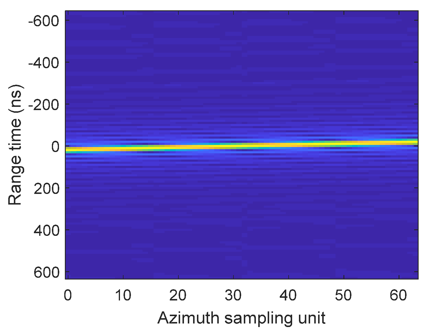
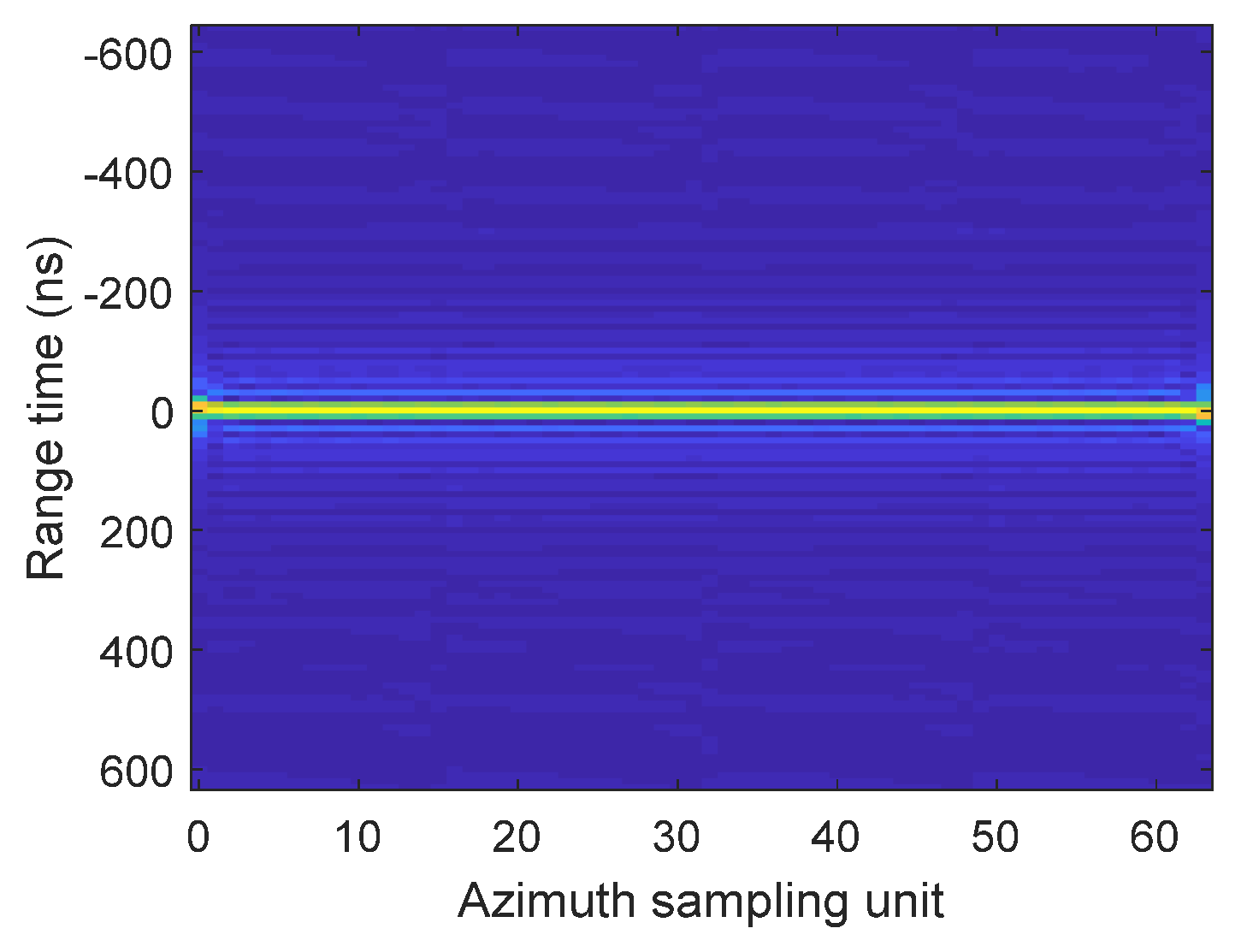
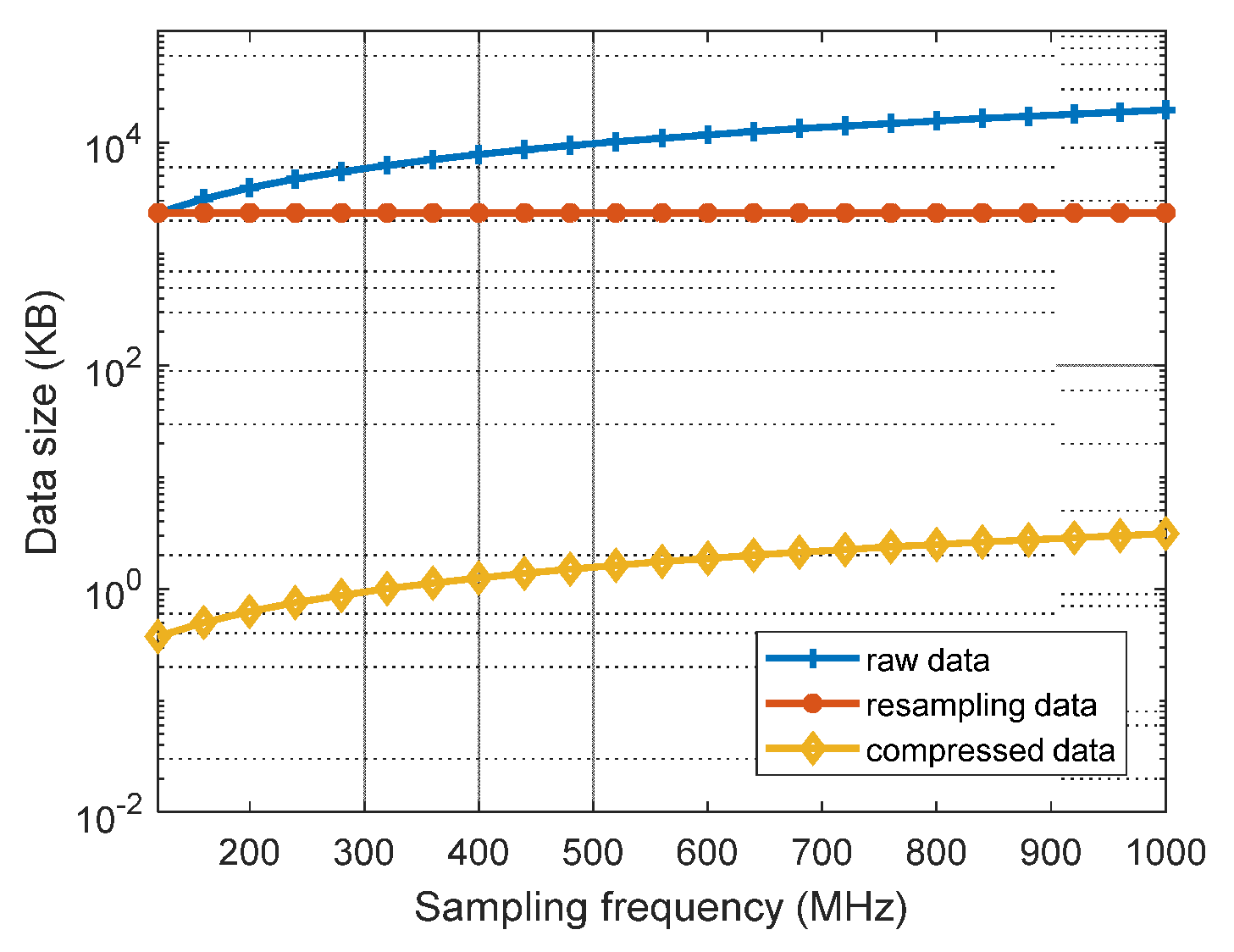
5.1. Data Compression Simulation

We simulated an LFM signal with the parameters given in

Table 2. Parameters of an LFM signal.

Parameters	Value
Carrier frequency	1.45 GHz
Bandwidth	50 MHz
Sampling frequency	100 MHz
Pulse repetition frequency	5 kHz
Pulse width	10 μs
Pulse number	64
SNR	5 dB

to verify the proposed method. After compressing the data in the range dimension, a slant line is obtained in the range-Doppler plane, as shown in Figure 6. The line shows that the TOA of the receiver is time-varying and reflects the true TOA during the movement. Since the RCM of the signal spans into multiple range cells, the modified Keystone transformation (e.g., (22)) is performed.

After the transformation, a horizontal straight line, as shown in Figure 7, is obtained. The range frequency and azimuth time are decoupled, and the data are well compressed in the azimuth dimension.

Figure 8 is the result after the azimuth compression. The red box indicates that the compressed data only occupies a small part of the range-Doppler plane. The data transmission is carried on after the azimuth compression. The data volume in the transmission is related to the width of the two first lobes of the compressed data, and the width is inversely proportional to the signal bandwidth in the range domain. Thus, the amount of data to be transmitted is significantly reduced for a wideband signal.

To compare the compression performance of the proposed method and a resampling method [32], we analyzed both outputs. Assuming that the azimuth sampling interval is T′, the sampling rate is F_s, the number of pulses is M, and the raw data transmission is MTF_s. The transmitted data in two methods are shown in Figure 9. B_r is 100 MHz, T is 100 µs, M is 100, and M_FFT is 10. Using 1.2 times B_r as the resampling frequency in the resampling method, the data transmission is still huge after resampling. It is because the signal bandwidth B_r limits the resampling frequency. As the data compression is inversely proportional to the signal bandwidth in the proposed method, the data transmission is very small for a wideband signal after the compression.

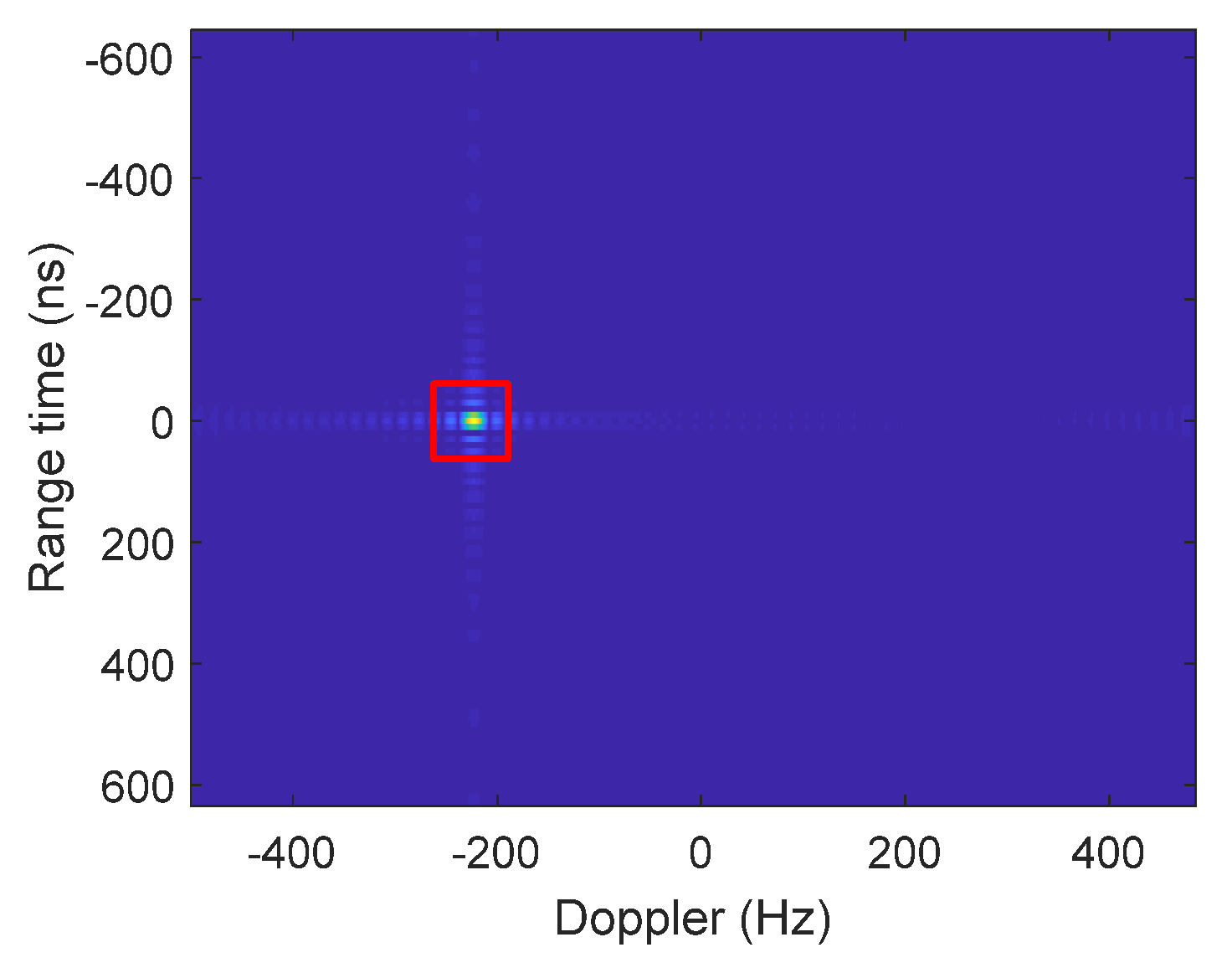
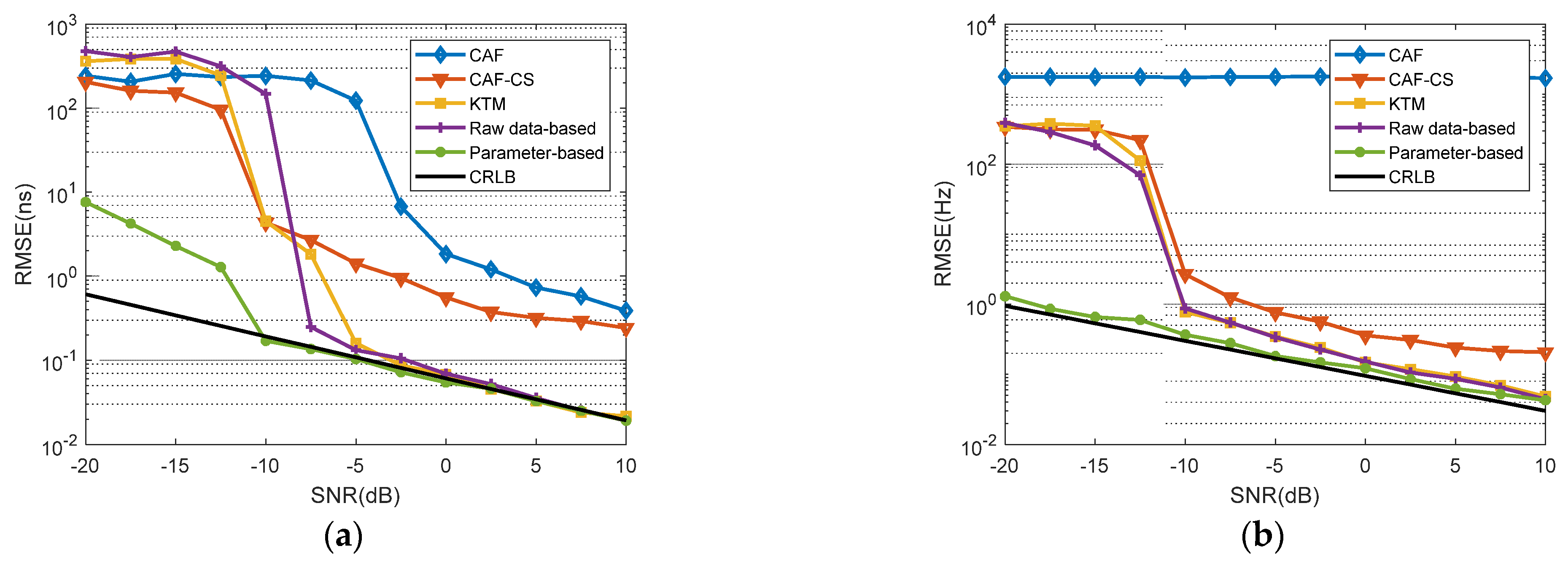
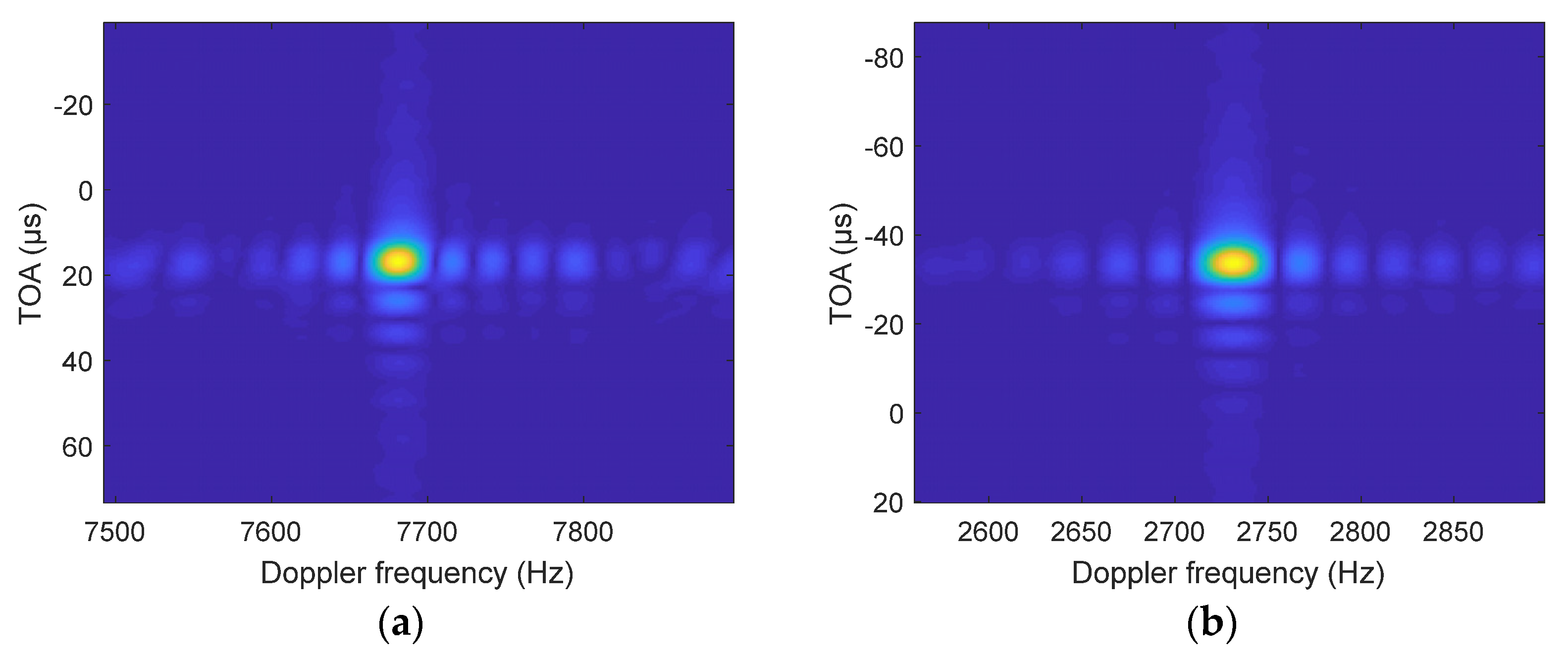
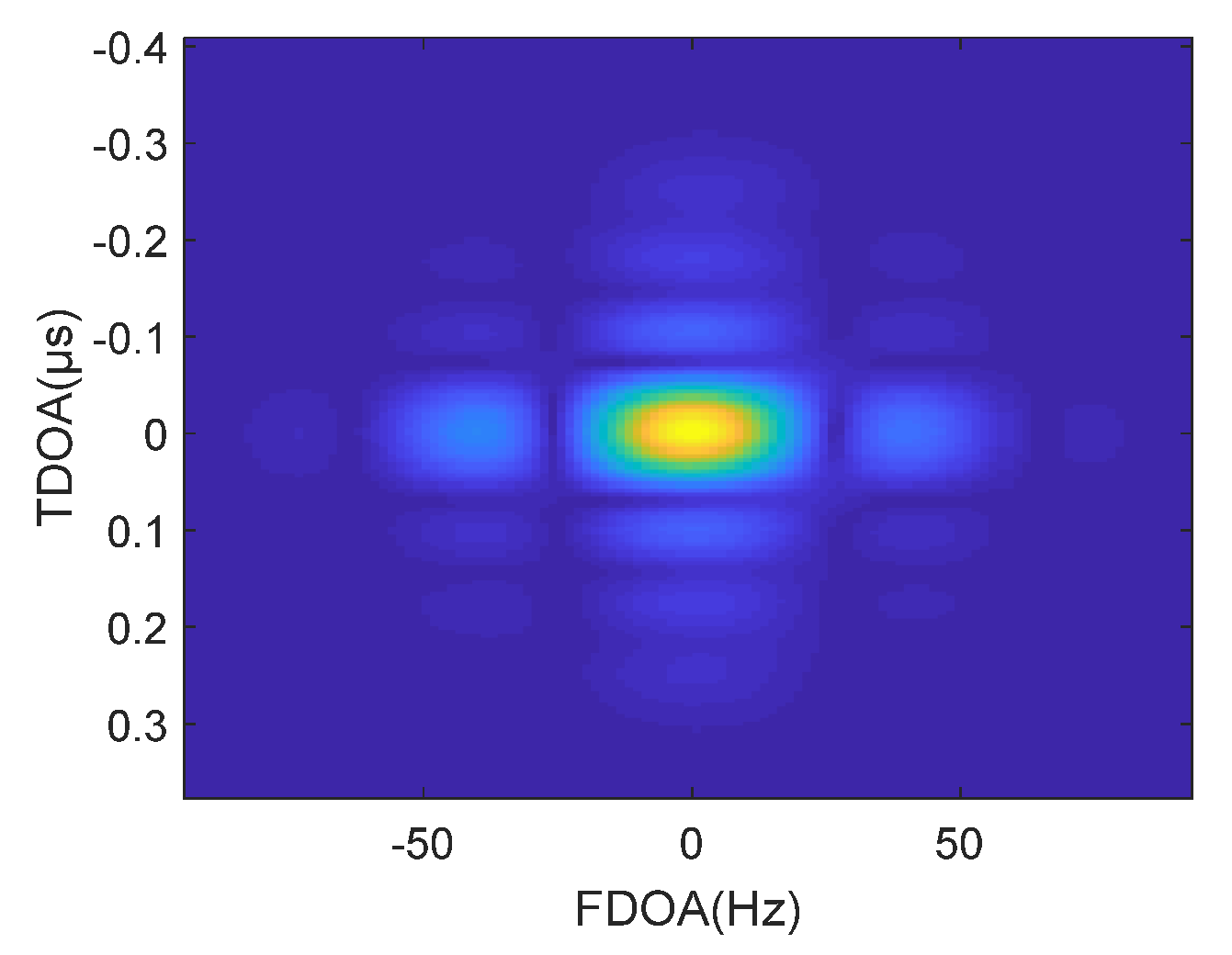
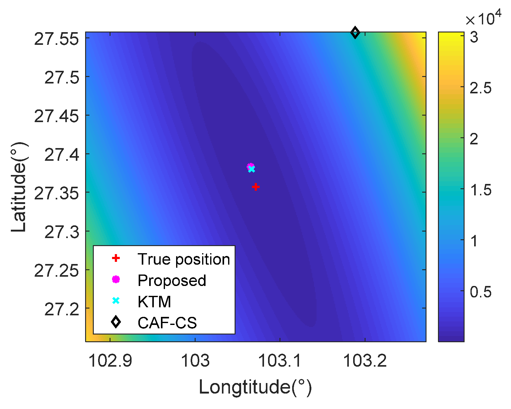
5.2. Numerical TDOA and FDOA Estimations

The MonteCarlo simulations were used to obtain the root-mean-square error (RMSE) of the proposed algorithm and traditional methods, including the CAF, CAF-CS, and KTM. The SNR varied from −20 to 10 dB with intervals of 2.5 dB. At each SNR value, 1000 simulations were run. The results of the raw data-based compression algorithm are shown in Figure 10. The proposed approach and KTM can reach the CRLB at high SNRs for the TDOA and FDOA estimations. Compared with the KTM, the proposed method does not require the entire data transmitted. Since the reference pulse in the raw data-based method is from the received signal, a noisy reference signal (e.g., SNR ≤ −7.5 dB) significantly degrades the performance in estimating the TDOA and the FDOA.

As the reference pulse by the parameter-based method does not contain noise, its overall performance of the TDOA and FDOA estimations is better than that of the raw data-based method. However, the raw data-based method can still be viable since an emitter’s system parameters are typically unknown. Thus, it is valuable that the applicability of the raw data-based method is articulated further, with the consideration of the input and output SNRs.

Assuming that size of the raw data was mn, and the compressed data size was m′n′. If the SNR for the input is SNR_in, the output SNR, SNR_out is

$$SN{R}_{out}=-10\lg (2\times {10}^{-\frac{SN{R}_{in}}{10}}+{10}^{-\frac{SN{R}_{in}}{5}})+10\lg (\frac{mn}{m^{\prime }{n}^{\prime }})$$

(53)

The derivation of (53) is detailed in Appendix C. The SNR_in and SNR_out relationship is shown in Figure 11. They have a positive relationship. It should be noted that when the reference pulse is noisy, the SNR_out decreases. Hence, the TDOA estimation performance deteriorates at a low SNR (e.g., Figure 10a).

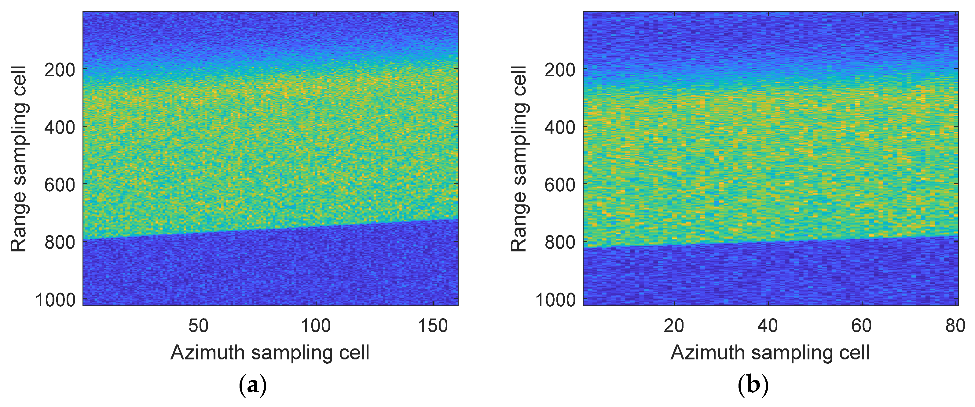
5.3. Hardware-In-The-Loop Data

We performed a hardware-in-the-loop simulation to examine the proposed method’s feasibility further. The signal parameter-based approach was adopted to complete the data compression since the signal parameters are known. The parameters are tabulated in

Table 3. Parameters of experimental data.

Parameters	Value
Central frequency	1.45 GHz
Bandwidth	20 MHz
Pulse width	4 μs
Pulse repetition frequency	10 kHz
Sampling rate	200 MHz

.

The true TDOA is 50.535 μs, and the true FDOA is 4944.670 Hz. An emitter was located at 103.0716°E and 27.3571°N. The orbital height of each satellite was 600 km. The nadir-view location of one satellite on the Earth’s surface was at 101.9216°E and 26.4271°N, and the nadir-view position of the second satellite was 102.8017°E and 26.6072°N. The computer sets the parameters of an LFM signal, and the hardware board completes the sending and receiving of the signal.

The raw data collected are in real data type. Since there is no phase information in the data of the real-data type, it may not be conducive. The Hilbert transform is used to obtain the phase information of the received signal. The results are shown in Figure 12.

Estimating the time difference and frequency difference is divided into two steps, data compression and joint processing. In the first step, the parameter-based compression algorithm compresses the received data from the two receivers. First, the Fourier transform is performed on the received data in the range dimension. Then, the reference function is constructed according to (27). After the received signal is multiplied by the reference function, the modified Keystone transformation is performed to correct the RCM. Finally, the inverse Fourier transform is performed in the range dimension, obtaining a range-dimensional compression result, as shown in Figure 13. The RCM correction is essential. Without it, the compression result is a slant line, resulting in a time-varying TDOA. After the correction, the accurate TOA at the central time can be obtained, as shown in Figure 14.

The azimuth Fourier transform completes the azimuth compression. The TOA and Doppler frequency of each receiver is then obtained, as shown in Figure 15. The data are well compressed. The TOA of Receiver #1 is 17.000 µs and the Doppler frequency is 7683.000 Hz. The TOA is −33.000 μs and the Doppler frequency is 2733.000 Hz for Receiver #2.

The received signal may be weak since a receiver is far away from the emitter. The SNR of the received signal may be very low, causing significant errors in the estimation results of the first step. The error can be reduced through the joint processing or the second step. The primary difference from traditional methods is that compressed data are used for joint processing. The data volume is tiny, and it is unnecessary to restore the compressed data to the original since accurate TDOA and FDOA are obtained with (33) and (34). The results are shown in Figure 16. The estimated TDOA and FDOA are 0.530 μs and −1.720 Hz, respectively. Thus, the TDOA and FDOA estimates are refined as 50.530 μs and 4948.280 Hz.

To quantify the performance of the proposed method, we compare it with the CAF-CS method and KTM. All raw data must be transferred when the CAF-CA method and KTM are used. The proposed method uses compressed data that have less than 0.2% of the original data volume (

Table 4. Size of the data matrix in transmission.

CAF-CS	KTM	Proposed
4096 × 80	4096 × 80	100 × 6

). Although the KTM has the best performance with the smallest TODA and FDOA errors (

Table 5. Results of experimental data.

	TDOA Error (ns)	FDOA Error (Hz)
CAF-CS	13.85	192.67
KTM	4.15	3.30
Proposed	5.00	3.61

), the proposed method still has a considerable advantage in scenarios when data-transmission bandwidth is limited.

Finally, the location of the emitter after the least-squares method is shown in Figure 17. The position is at 103.0659°E and 27.3837°N. The positioning error is −0.0057° in longitude and 0.0266° in latitude.

6. Discussion

Typically, the sampling rate satisfies Nyquist’s law to sample the passive signal without distortion. However, wideband sources such as ISAR radar transmit signals with a bandwidth of several hundred MHZ to several GHz, resulting in a large volume of data to be collected by the receiver. If the receiver is placed on a satellite platform, data transmission will be a challenge. Fortunately, radar equipment generally transmits coherent pulses, and the method proposed in this paper is well suited for this environment. Future research will be conducted to recover signal coherence so that the methods in this paper can be applied to more signal types.

When the intercepted signal is completely unknown, the received signal is used directly as a reference function (Method A). In this case, the processing results of the proposed algorithm are consistent with that of the traditional algorithm based on the cross-correlation function, and the interference is not filtered. When the received signal is known, the coherent accumulation of the received signal can be achieved by the reference function constructed by the signal parameters (Method B), and the interference is filtered. Therefore, the proposed method has good interference immunity in the localization of known signals.

7. Conclusions

A multi-pulse cross ambiguity function (MPCAF) was proposed to reduce the data volume in transmission when two spaceborne receivers were used to locate an emitter on the ground passively. It consists of the coarse time difference of arrival (TDOA) and frequency difference of arrival (FDOA) estimations with data compression and refined estimation with the joint processing. In the coarse estimations, two methods, a raw data-based method and a signal data-based one, were proposed to create the reference pulse, and the raw data were then compressed. In the raw data-based method, the reference pulse is directly constructed from the received data, which can be noisy. The reference pulse in a signal parameter-based method contains no noise. Both methods have the same performance at a high SNR, but the performance of the raw data-based method deteriorates as the SNR decreases. The wideband signal is significantly compressed with the compression methods to reduce the volume in data transmission. To refine the TDOA and DFOA estimations, we proposed the joint processing with a wideband cross-correlation function, achieving accurate estimations. Simulations show that the performance of the proposed method reaches the Cramer–Rao lower bound. The hardware-in-the-loop simulation also validates the effectiveness of the proposed method.

The relative motion speed presented in this paper is constant, and the received signal has a Doppler shift in the azimuth. When the relative speed is not constant, the signal has multiple Doppler frequency components, resulting in a multi-valued FDOA of MPCAF. Fortunately, this situation is very similar to the Doppler spectrum in SAR imaging. The center of the spectrum is uniquely determined and can be estimated (e.g., the Map–Drift method). Further work will consider the situation where the short aperture assumption is not satisfied. In this situation, relative motion velocity varies with the view angle, and the signal occupies multiple Doppler sampling units. The subsequent work will deal with the issue.

References

1. Zou, Y.; Wan, Q. Asynchronous Time-of-Arrival-Based Source Localization with Sensor Position Uncertainties. IEEE Commun. Lett. 2016, 20, 1860–1863. [Google Scholar] [CrossRef]
2. Shen, H.; Ding, Z.; Dasgupta, S.; Zhao, C. Multiple Source Localization in Wireless Sensor Networks Based on Time of Arrival Measurement. IEEE Trans. Signal Process. 2014, 62, 1938–1949. [Google Scholar] [CrossRef]
3. Ricciato, F.; Sciancalepore, S.; Gringoli, F.; Facchi, N.; Boggia, G. Position and Velocity Estimation of a Non-Cooperative Source from Asynchronous Packet Arrival Time Measurements. IEEE Trans. Mob. Comput. 2018, 17, 2166–2179. [Google Scholar] [CrossRef]
4. Nogueira, L.C.F.; Petraglia, M.R. Robust localization of multiple sound sources based on BSS algorithms. In Proceedings of the 2015 IEEE 24th International Symposium on Industrial Electronics (ISIE), Rio de Janeiro, Brazil, 3–5 June 2015; pp. 579–583. [Google Scholar]
5. Pattison, T.; Chou, S.I. Sensitivity analysis of dual-satellite geolocation. IEEE Trans. Aerosp. Electron. Syst. 2000, 36, 56–71. [Google Scholar] [CrossRef]
6. Amishima, T.; Wakayama, T.; Okamura, A.; Okamura, A. TDOA association for localization of multiple emitters when each sensor receives different number of incoming signals. In Proceedings of the 2014 Proceedings of the SICE Annual Conference (SICE), Sapporo, Japan, 9–12 September 2014; pp. 1656–1661. [Google Scholar] [CrossRef]
7. Park, C.; Chang, J. Robust TOA source localisation algorithm using prior location. IET Radar Sonar Navig. 2019, 13, 384–391. [Google Scholar] [CrossRef]
8. Ho, K.C.; Wenwei, X. An accurate algebraic solution for moving source location using TDOA and FDOA measurements. IEEE Trans. Signal Process. 2004, 52, 2453–2463. [Google Scholar] [CrossRef]
9. Vidal-Valladares, M.G.; Díaz, M.A. A Femto-Satellite Localization Method Based on TDOA and AOA Using Two CubeSats. Remote Sens. 2022, 14, 1101. [Google Scholar] [CrossRef]
10. Zhou, T.; Yi, W.; Kong, L. Non-Cooperative Passive Direct Localization Based on Waveform Estimation. Remote Sens. 2021, 13, 264. [Google Scholar] [CrossRef]
11. Devaney, A. Time reversal imaging of obscured targets from multistatic data. IEEE Trans. Antennas Propag. 2005, 53, 1600–1610. [Google Scholar] [CrossRef]
12. Prada, C.; Fink, M. Eigenmodes of the time reversal operator: A solution to selective focusing in multiple-target media. Wave Motion 1994, 20, 151–163. [Google Scholar] [CrossRef]
13. Marengo, E.A.; Gruber, F.K.; Simonetti, F. Time-Reversal MUSIC Imaging of Extended Targets. IEEE Trans. Image Process. 2007, 16, 1967–1984. [Google Scholar] [CrossRef]
14. Ciuonzo, D. On Time-Reversal Imaging by Statistical Testing. IEEE Signal Process. Lett. 2017, 24, 1024–1028. [Google Scholar] [CrossRef] [Green Version]
15. Hu, D.; Huang, Z.; Liang, K.; Zhang, S. Coherent TDOA/FDOA estimation method for frequency-hopping signal. In Proceedings of the 2016 8th International Conference on Wireless Communications & Signal Processing (WCSP), Yangzhou, China, 13–15 October 2016; pp. 1–5. [Google Scholar]
16. Wang, Y.; Ho, K.C. TDOA Positioning Irrespective of Source Range. IEEE Trans. Signal Process. 2017, 65, 1447–1460. [Google Scholar] [CrossRef]
17. Liu, Y.; Guo, F.; Yang, L.; Jiang, W. An Improved Algebraic Solution for TDOA Localization with Sensor Position Errors. IEEE Commun. Lett. 2015, 19, 2218–2221. [Google Scholar] [CrossRef]
18. Wei, H.-W.; Peng, R.; Wan, Q.; Chen, Z.-X.; Ye, S.-F. Multidimensional Scaling Analysis for Passive Moving Target Localization with TDOA and FDOA Measurements. IEEE Trans. Signal Process. 2010, 58, 1677–1688. [Google Scholar] [CrossRef]
19. Wang, Y.; Wu, Y. An Efficient Semidefinite Relaxation Algorithm for Moving Source Localization Using TDOA and FDOA Measurements. IEEE Commun. Lett. 2017, 21, 80–83. [Google Scholar] [CrossRef]
20. Zhou, L.; Zhu, W.; Luo, J.; Kong, H. Direct positioning maximum likelihood estimator using TDOA and FDOA for coherent short-pulse radar. IET Radar, Sonar Navig. 2017, 11, 1505–1511. [Google Scholar] [CrossRef]
21. Wang, G.; Cai, S.; Li, Y.; Ansari, N. A Bias-Reduced Nonlinear WLS Method for TDOA/FDOA-Based Source Localization. IEEE Trans. Veh. Technol. 2016, 65, 8603–8615. [Google Scholar] [CrossRef]
22. Noroozi, A.; Oveis, A.H.; Hosseini, S.M.; Sebt, M.A. Improved Algebraic Solution for Source Localization from TDOA and FDOA Measurements. IEEE Wirel. Commun. Lett. 2018, 7, 352–355. [Google Scholar] [CrossRef]
23. Amar, A.; Weiss, A.J. Optimal radio emitter location based on the Doppler effect. In Proceedings of the 2008 5th IEEE Sensor Array and Multichannel Signal Processing Workshop, Darmstadt, Germany, 21–23 July 2008; pp. 54–57. [Google Scholar]
24. Guo, F.; Zhang, Z.; Yang, L. TDOA/FDOA estimation method based on dechirp. IET Signal Process. 2016, 10, 486–492. [Google Scholar] [CrossRef]
25. Stein, S. Algorithms for ambiguity function processing. IEEE Trans. Acoust. Speech Signal Process. 1981, 29, 588–599. [Google Scholar] [CrossRef]
26. Betz, J. Effects of uncompensated relative time companding on a broad-band cross correlator. IEEE Trans. Acoust. Speech Signal Process. 1985, 33, 505–510. [Google Scholar] [CrossRef]
27. Zhang, L.; Yang, B.; Luo, M. Joint Delay and Doppler Shift Estimation for Multiple Targets Using Exponential Ambiguity Function. IEEE Trans. Signal Process. 2017, 65, 2151–2163. [Google Scholar] [CrossRef]
28. Ulman, R.; Geraniotis, E. Wideband TDOA/FDOA processing using summation of short-time CAF’s. IEEE Trans. Signal Process. 1999, 47, 3193–3200. [Google Scholar] [CrossRef]
29. Xiao, X.; Guo, F.; Feng, D. Low-complexity methods for joint delay and Doppler estimation of unknown wideband signals. IET Radar Sonar Navig. 2018, 12, 398–406. [Google Scholar] [CrossRef]
30. Yeredor, A.; Angel, E. Joint TDOA and FDOA Estimation: A Conditional Bound and Its Use for Optimally Weighted Localization. IEEE Trans. Signal Process. 2011, 59, 1612–1623. [Google Scholar] [CrossRef]
31. Stein, S. Differential delay/Doppler ML estimation with unknown signals. IEEE Trans. Signal Process. 1993, 41, 2717–2719. [Google Scholar] [CrossRef]
32. Kim, D.-G.; Park, G.-H.; Kim, H.-N.; Park, J.-O.; Park, Y.-M.; Shin, W.-H. Computationally Efficient TDOA/FDOA Estimation for Unknown Communication Signals in Electronic Warfare Systems. IEEE Trans. Aerosp. Electron. Syst. 2018, 54, 77–89. [Google Scholar] [CrossRef]
33. Darsena, D.; Gelli, G.; Iudice, I.; Verde, F. Detection and blind channel estimation for UAV-aided wireless sensor networks in smart cities under mobile jamming attack. IEEE Internet Things J. 2022, 9, 11932–11950. [Google Scholar] [CrossRef]
34. Kelner, J.M.; Ziółkowski, C. Effectiveness of Mobile Emitter Location by Cooperative Swarm of Unmanned Aerial Vehicles in Various Environmental Conditions. Sensors 2020, 20, 2575. [Google Scholar] [CrossRef]
35. Chen, J.; Zhang, J.; Jin, Y.; Yu, H.; Liang, B.; Yang, D.-G. Real-Time Processing of Spaceborne SAR Data with Nonlinear Trajectory Based on Variable PRF. IEEE Trans. Geosci. Remote Sens. 2022, 60, 1–12. [Google Scholar] [CrossRef]
36. Sun, G.-C.; Xing, M.; Xia, X.-G.; Wu, Y.; Bao, Z. Beam Steering SAR Data Processing by a Generalized PFA. IEEE Trans. Geosci. Remote Sens. 2013, 51, 4366–4377. [Google Scholar] [CrossRef]
37. Liu, Y.; Sun, G.-C.; Guo, L.; Xing, M.; Yu, H.; Fang, R.; Wang, S. High-Resolution Real-Time Imaging Processing for Spaceborne Spotlight SAR With Curved Orbit via Subaperture Coherent Superposition in Image Domain. IEEE J. Sel. Top. Appl. Earth Obs. Remote Sens. 2022, 15, 1992–2003. [Google Scholar] [CrossRef]
38. Wu, Y.; Sun, G.; Xia, X.-G.; Xing, M.; Bao, Z. An Improved SAC Algorithm Based on the Range-Keystone Transform for Doppler Rate Estimation. IEEE Geosci. Remote Sens. Lett. 2013, 10, 741–745. [Google Scholar] [CrossRef]
Figure 1. The geometry of two receivers and an emitter.
Remotesensing 14 03545 g001
Figure 2. The flowchart of the TDOA and FDOA estimations.
Remotesensing 14 03545 g002
Figure 3. TDOA at different azimuth times. (a) With reference pulse at zero time, (b) With reference pulse at tm0.
Remotesensing 14 03545 g003
Figure 4. Refining TDOA and FDOA estimations.
Remotesensing 14 03545 g004
Figure 5. Spectrum aliasing.
Remotesensing 14 03545 g005
Figure 6. Result of a raw data-based method of Receiver #1.
Remotesensing 14 03545 g006
Figure 7. The result after the modified Keystone transformation.
Remotesensing 14 03545 g007
Figure 8. The result after the azimuth compression.
Remotesensing 14 03545 g008
Figure 9. Data transmission in two methods.
Remotesensing 14 03545 g009
Figure 10. RMSEs of five methods. (a) RMSE of the TDOA estimation, (b) RMSE of the FDOA estimation.
Remotesensing 14 03545 g010
Figure 11. Relationships of input and output SNRs.
Remotesensing 14 03545 g011
Figure 12. Raw (in complex-data type) of two receivers. (a) Receiver #1, (b) Receiver #2.
Remotesensing 14 03545 g012
Figure 13. Compression result without the RCM correction. (a) Receiver #1, (b) Receiver #2.
Remotesensing 14 03545 g013
Figure 14. TOAs of two receivers after the RCM correction. (a) Receiver #1, (b) Receiver #2.
Remotesensing 14 03545 g014
Figure 15. Two-dimensional compression result. (a) Receiver #1, (b) Receiver #2.
Remotesensing 14 03545 g015
Figure 16. Results after joint processing.
Remotesensing 14 03545 g016
Figure 17. Locating results.
Remotesensing 14 03545 g017