JPSS VIIRS SST Reanalysis Version 3

Abstract

The 3rd full-mission reanalysis (RAN3) of global sea surface temperature (SST) with a 750 m resolution at nadir is available from VIIRS instruments flown onboard two JPSS satellites: NPP (February 2012–present) and N20 (January 2018–present). Two SSTs, ‘subskin’ (sensitive to skin SST) and ‘depth’ (proxy for in situ SST at depth of 20 cm), were produced from brightness temperatures (BTs) in the VIIRS bands centered at 8.6, 11 and 12 µm during the daytime and an additional 3.7 µm band at night, using the NOAA Advanced Clear Sky Processor for Ocean (ACSPO) enterprise SST system. The RAN3 dataset is fully archived at NASA JPL PO.DAAC and NOAA CoastWatch, and routinely supplemented in near real time (NRT) with a latency of a few hours. Delayed mode (DM) processing with a 2 months latency follows NRT, resulting in a more uniform science quality SST record. This paper documents and evaluates the performance of the VIIRS RAN3 dataset. Comparisons with in situ SSTs from drifters and tropical moorings (D+TM) as well as Argo floats (AFs) (both available from the NOAA iQuam system) show good agreement, generally within the NOAA specifications for accuracy (±0.2 K) and precision (0.6 K), in a clear-sky domain covering 18–20% of the global ocean. The nighttime SSTs compare with in situ data more closely, as expected due to the reduced diurnal thermocline. The daytime SSTs are also generally within NOAA specs but show some differences between the (D+TM) and AF validations as well as residual drift on the order of −0.1 K/decade. BT comparisons between two VIIRSs and MODIS-Aqua show good consistency in the 3.7 and 12 µm bands. The 11 µm band, while consistent between NPP and N20, shows residual drift with respect to MODIS-Aqua. Similar analyses of the 8.6 µm band are inconclusive, as the performance of the MODIS band 29 centered at 8.6 µm is degraded and unstable in time and cannot be used for comparisons.

1. Introduction

The National Oceanic and Atmospheric Administration (NOAA) provides sea surface temperature (SST) retrievals from multiple earth-observing satellites using its Advanced Clear Sky Processor for Ocean (ACSPO) enterprise SST system. ACSPO SST products are available from VIIRS, MODIS, AVHRR GAC and FRAC sensors flown onboard multiple low earth orbiting (LEO; including NPP/N20, Aqua/Terra, NOAA-7/9/11/12/14/15/16/17/18/19 and Metop-A/B/C) and from the ABI and AHI sensors flown onboard geostationary (GOES-16/17/18 and Himawari-8) satellites [1,2,3,4,5,6].

The first VIIRS instrument was launched onboard the NPP satellite on 28 October 2011, and its SST data became available on 1 February 2012 [7,8]. The second VIIRS was launched onboard NOAA-20 (N20; aka JPSS-1, or J1, prelaunch) on 18 November 2017, and its SST data became available on 5 January 2018 [9,10]. NPP and N20 are part of the NOAA Joint Polar Satellite System (JPSS) and fly in the same Sun-synchronous ‘afternoon’ (PM) orbits, lagged by 50 min, with 1:30 am/pm local equator crossing times (LEXTs). Stable orbits are maintained by execution of periodical orbital corrections using onboard fuel. Due to the large VIIRS swath width of ~3000 km, there are no gaps in coverage at the equator between consecutive orbits. As a result, the NPP and N20 VIIRSs independently provide global coverage, at least twice every 24 h. Future satellites in the JPSS constellation (JPSS-2/3/4) will continue carrying VIIRS sensors in the same orbit, with the next satellite in the series (JPSS-2/N21) planned for launch in September 2022.

ACSPO produces SSTs from clear-sky brightness temperatures (BTs) in VIIRS moderate resolution bands. ACSPO VIIRS level 2 products (L2P) are provided in the original sensor spatial resolution 750 m at nadir degrading to 1500 m at the swath edge [11]. Due to the large L2P data size, a reduced-volume L3U (gridded uncollated) product is also produced by mapping L2P data onto 0.02° equal grid [4]. Both L2P and L3U ACSPO data are provided as 10 min granules (144 files/24 h/sensor) compliant with the Group for High Resolution SST (GHRSST) Data Specification version 2 (GDS2) standard [12]. For users interested in further reduced data volume and increased information density, a super-collated L3S-LEO ‘PM’ product is available, where L3U data from NPP and N20 are combined (collated) into a multisensor product [13,14,15]. All ACSPO VIIRS SST data are available back to the earliest available high-quality L1b data in thermal infrared (IR) bands (1 February 2012 for NPP and 5 January 2018 for N20), with new data added in near real time (NRT) with a latency of 1–3 h for L2P/L3U and 3–6 h for L3S. Delayed-mode (DM) processing follows NRT with a latency of two months, resulting in a higher quality SST, more consistent with full-mission reanalysis (RAN) data. Complete archives of the VIIRS L2P, L3U and L3S data are available at the NASA Physical Oceanography Distributed Active Archive Center (PO.DAAC) [7,8,9,10,15]. ACSPO VIIRS data are also archived at the NOAA CoastWatch [16,17]. However, due to the data storage limitations, CoastWatch reports complete records of only L3U and L3S data, while L2P NRT data are only available as a two most recent weeks rotated buffer. Global performance of ACSPO VIIRS SST against in situ and L4 SSTs is monitored in the NOAA SST Quality Monitor (SQUAM) online system [18]. Regional performance, including quality of the SST imagery and ACSPO Clear Sky Mask (ACSM), is monitored in the ACSPO Regional Monitor for SST (ARMS) online system [19]. (Please note that in ACSPO, the ‘clear-sky mask’ term is used instead of the often used ‘cloud mask’ term, to emphasize the fact that pixels can be excluded for reasons other than obstruction by cloud, e.g., heavy aerosol contamination, invalid SST retrievals and sensor issues.)

The goal of the VIIRS RAN is reprocessing all available VIIRS L1b data and creating a uniform time series of ACSPO SST back to the beginning of all satellite missions carrying VIIRS sensors (currently, NPP and N20). This work documents the VIIRS RAN3 dataset produced using ACSPO V2.80. VIIRS RAN1 was performed in 2015 with ACSPO V2.40, and RAN2 in 2019 with ACSPO V2.61 [20]. (Note that in this paper, RAN1/2/3 refer to the datasets and V2.40/2.61/2.80 to the versions of ACSPO system used to produce them.) RAN2 introduced improved thermal band calibration, which addressed positive SST biases (up to 0.3 K globally) resulting from quarterly (yearly after June 2018) warm-up cool-down (WUCD) exercises performed by the VIIRS calibration team [21,22]. RAN2 also introduced improved SST imagery (by correcting bow-tie distortions and deletions [23]) and more accurate SST retrievals (taking advantage of the VIIRS M14 band, centered at 8.6 µm [20]). RAN3 further improves upon RAN2, by mitigating warm SST biases in the high latitudes and reducing false positive cloud detection in dynamic areas such as the Gulf Stream. RAN3 also introduces two new thermal fronts layers (location of fronts, and their intensity in units of K/km). Compared to RAN2, the L2P data volume in RAN3 was reduced by a factor of 4 (from 10 to 2.5 TB/year/sensor). This is achieved by removing BTs from the ACSPO files, increasing the compression level and truncating unphysical retrieved SST values below −2 °C (typically retrieved over cold clouds).

This work is organized as follows. Section 2 provides an overview of the ACSPO algorithm, with an emphasis on the improvements and new additions in RAN3 (produced with ACSPO V2.80) compared to RAN2 (produced with ACSPO V2.61). Section 3 presents the results of the validation of ACSPO VIIRS SSTs against quality-controlled in situ data from the NOAA in situ Quality Monitor (iQuam) system [24,25]. The nighttime SST validation biases are found to be stable in time and consistent between NPP and N20, whereas the daytime retrievals show an unphysical near linear trend of ~−0.01 K/year. Section 4 analyzes the causes of the daytime trend and evaluates the stability of the VIIRS thermal emissive bands by comparing the NPP/N20 VIIRS BTs with MODIS-Aqua BTs, using the modeled BTs (with the community radiative transfer model, CRTM) as a ‘transfer standard’ [26,27]. Section 4 summarizes the results of this study and discusses future work.

2. ACSPO Algorithms

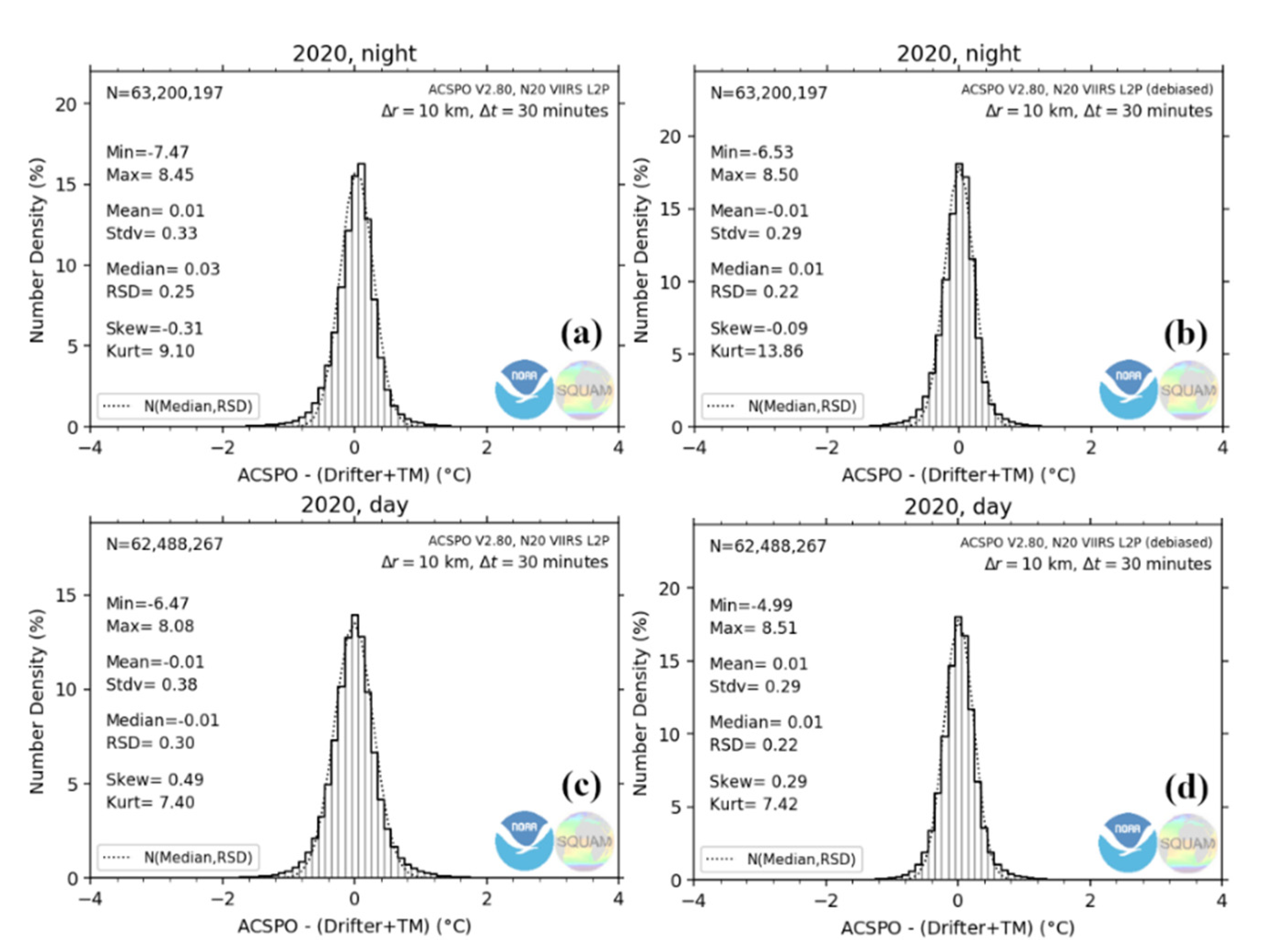
ACSPO retrieves SSTs from clear-sky BTs in VIIRS moderate resolution, M-bands centered at 3.7 (M12), 8.6 (M14), 10.8 (M15) and 12.0 µm (M16) [2,3]. Additionally, three reflective solar bands centered at 0.67 (M5), 0.86 (M7) and 1.61 µm (M10) are used in the daytime ACSM [1]. ACSPO reports ‘subskin’ SST (in the ‘sea_surface_temperature’ layer), from which ‘depth’ SST can be derived by subtracting the sensor specific error statistics (SSES) bias (in the text below, the ‘depth’ SST is also referred to as ‘debiased’ SST). The ‘subskin’ SST is the sea temperature at depth of ~1 mm, and ‘depth’ SST is a proxy for SST at depth typically sampled by drifting buoys (~20 cm) [12]. Both ‘subskin’ and ‘depth’ SSTs are calculated using the nonlinear SST (NLSST) algorithms [2,28]. During the daytime, a three-band equation is used in the following form:

$$\begin{array}{cc}{T}_S=& a_0+a_1{T}_{11}+a_2\left(T_{11}-T_{8.6}\right)+a_3\left(T_{11}-T_{12}\right)+a_4{T}_{11}S+a_5\left(T_{11}-T_{8.6}\right)S+a_6\left(T_{11}-T_{12}\right)S\\ & +a_7\left(T_{11}-T_{8.6}\right)T_0+a_8\left(T_{11}-T_{12}\right)T_0+a_{9}S. \end{array}$$

(1)

At night, a four-band equation, with an additional 3.7 µm band, is used:

$$\begin{array}{cc}{T}_S=b_0+b_1{T}_{11}& +b_2\left(T_{11}-T_{3.7}\right)+b_3\left(T_{11}-T_{8.6}\right)+b_4\left(T_{11}-T_{12}\right)+b_5{T}_{11}S+b_6\left(T_{11}-T_{3.7}\right)+b_7\left(T_{11}-T_{8.6}\right)S\\ & +b_8\left(T_{11}-T_{12}\right)+b_9\left(T_{11}-T_{3.7}\right)T_0+b_{10}\left(T_{11}-T_{8.6}\right)T_0+b_{11}\left(T_{11}-T_{12}\right)+b_{12}S.\end{array}$$

(2)

Here, T_3.7, T_8.6, T₁₁ and T₁₂ are BTs in the VIIRS thermal bands centered at 3.7, 8.6, 10.8 and 12 µm; $S=sec\left(\theta \right)-1$, with θ being the satellite view zenith angle (VZA); $a_i$ and $b_i$ are the regression coefficients, trained against iQuam in situ SSTs from drifting buoys and tropical moorings (D+TM) using one full year of matchups in 2018. During the daytime (solar zenith angle, SZA < 90°), the 3.7 µm band is excluded due to the contribution from reflected solar light.

The multiple ‘atmospheric’ terms with BT differences (BTDs) in Equations (1) and (2) introduce additional noise in the retrieved SSTs [29], which may be suppressed using a moving average (assuming that BTDs mainly contain atmospheric signals [30]). In reality, BTDs may also contain some information about SST, which should be retained to avoid the loss of sensitivity of retrieved SST to true SST [30]. The ACSPO algorithm [31] attempts to account for both atmospheric and SST signals by (1) extracting the ‘SST-correlated component’ from BTDs (calculated by correlation with the lead band, T₁₁); (2) suppressing noise in the ‘BTD residual’ using smoothing within a spatial window of 11 × 11 pixels; (3) adding the ‘noise-free BTD residual’ back to the ‘SST-correlated component’.

Note that the ACSPO Equations (1) and (2) have the same NLSST form as for AVHRR and MODIS SSTs, except they use the 8.6 µm band available on VIIRS [5]. Inclusion of the VIIRS 8.6 µm band improves retrieved SST in terms of precision (standard deviation with respect to in situ SST) and sensitivity to true SST [2] (especially during the daytime, when the more atmospherically transparent 3.7 µm band is not available). AVHRRs do not have the 8.6 µm band, and while MODIS instruments have a similar band 29, its performance is degraded on both Aqua and Terra [32] and, therefore, it is not used in ACSPO MODIS products.

Two sets of regression coefficients (one for day and one for night) are used to retrieve ‘subskin’ SSTs in the full global clear-sky domain (the ACSPO ‘subskin’ SSTs may be also referred to as global regression, GR, SST in the text below). The ‘depth’ SST is calculated using the same NLSST Equations (1) and (2) but using a piecewise regression (PWR) algorithm [3], where the retrieval domain is split into multiple segments, each with its own set of regression coefficients. The delta between ‘subskin’ and ‘depth’ SSTs is stored in ACSPO GDS2 files in the variable ‘sses_bias’, and the ‘depth’ SST can be obtained by subtracting the ‘sses_bias’ from the ‘subskin’ SST.

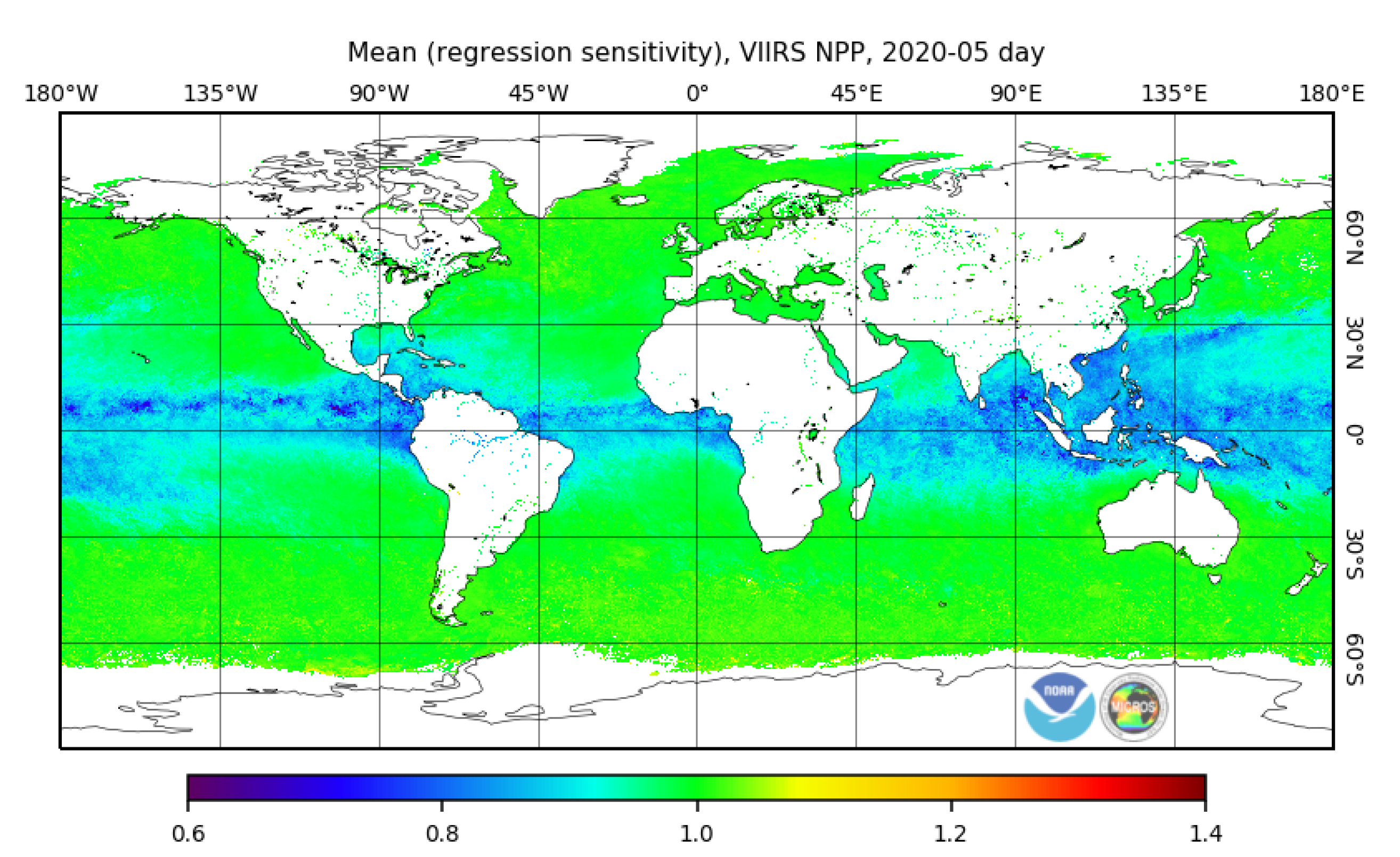
Both ‘subskin’ and ‘depth’ SST regression coefficients are trained against quality-controlled iQuam in situ (D+TM) SSTs and, therefore, both have a global mean bias of zero with respect to in situ (depth) SST on the training dataset. The main difference between the ACSPO ‘subskin’ and ‘depth’ SSTs is that the ‘subskin’ SST is more sensitive to spatial and temporal variations in skin SST (with a mean sensitivity of 0.99 for the VIIRS nighttime and 0.96 for the daytime ‘subskin’ SST). (Note that sensitivity is calculated by differentiating Equations (1) and (2) with respect to SST, with partial derivatives of BTs computed using a radiative transfer model. For a more detailed discussion of the role of sensitivity in ACSPO SST algorithms, we refer the reader to Reference [2]).

Figure 1 shows that the lower daytime sensitivity comes from tropical regions, especially at high VZAs, where thermal IR radiation is more strongly absorbed, due to the large concentrations of water vapor. As will be shown in Section 3, the ACSPO ‘depth’ SSTs have improved accuracy and precision against in situ SSTs. However, their improved performance statistics come at a cost of reduced sensitivity to true SST (approximately 0.6; cf. [5]).

Below, we estimate each band’s relative contribution to (or load on) the SST, according to Equations (1) and (2). These estimates are particularly interesting in the context of using the 8.6 µm band in ACSPO (recall that this band is not used in VIIRS SSTs produced by JPL [33,34] or NAVO [35,36]). To that end, we computed global mean values of partial derivatives of the NLSST Equations (1) and (2) wrt BT in each band. Note that these derivatives are not constant due to the presence of angular (VZA) and first-guess SST (T₀) terms; thus, averaging over the entire NPP and N20 missions was performed. As an example, the daytime contribution of the 12 µm band is computed by taking the partial derivative of Equation (1) wrt T₁₂ and averaging the resulting expression (denoted by angular brackets), giving $\langle \partial T_S/\partial T_{12}\rangle =-a_3-a_6\langle S\rangle -a_8\langle T_0\rangle$. The same approach was used to estimate the contribution of the first-guess SST, by taking a partial derivative wrt T₀.

Table 1. Loads (partial derivatives averaged over full NPP and N20 missions) on all bands and on the first-guess SST in the nighttime NLSST Equation (2). Corresponding SDs are also shown.

Night	T3.7	T8.6	T11	T12	T0
Mean (NPP)	1.340	−0.132	0.471	−0.666	−0.0002
Mean (N20)	1.339	−0.129	0.474	−0.671	−0.0007
SD (NPP)	0.047	0.102	0.107	0.121	0.0087
SD (N20)	0.046	0.101	0.105	0.119	0.0083

shows that the dominant contribution to nighttime SSTs, +1.34, comes from the most atmospherically transparent 3.7 µm band. The next highest weights, −0.67 and +0.47, are on the 12 µm band (the one most affected by water vapor absorption) and the more transparent 11 µm band, respectively. The load on the 8.6 µm band, −0.13, is smallest, out of all four bands at night, and the load on the first-guess SST is < ±0.001.

Table 2. Same as in Table 1 but for daytime SSTs produced with Equation (1).

Day	T3.7	T8.6	T11	T12	T0
Mean (NPP)	-	0.757	2.886	−2.562	−0.0005
Mean (N20)	-	0.750	2.801	−2.469	−0.0030
SD (NPP)	-	0.163	0.356	0.346	0.0263
SD (N20)	-	0.153	0.345	0.313	0.0212

shows the corresponding daytime results. All individual loads are much higher than at night. This is due to the longwave IR bands being less sensitive to SST than the 3.7 µm band. As expected, the largest load is on the 11 µm (+2.85) and 12 µm (−2.50) bands. Importantly, the contribution of the 8.6 µm band is also significant (+0.75), approximately a quarter of the 11 and 12 µm bands. The higher loads make daytime SST retrievals more sensitive to errors/drifts in individual BTs, which may be amplified (if not correlated between different bands and do not offset each other). Although daytime mean loads on first-guess SST are slightly larger than at night, in a globally average sense, they remain substantially smaller compared to the BT loads, suggesting that retrieved SSTs remain largely insensitive to first-guess SST. Note that the sensitivity of daytime SSTs to first-guess SST is more variable in space (cf. their higher SDs; e.g., daytime 0.026 vs. nighttime 0.009 for NPP).

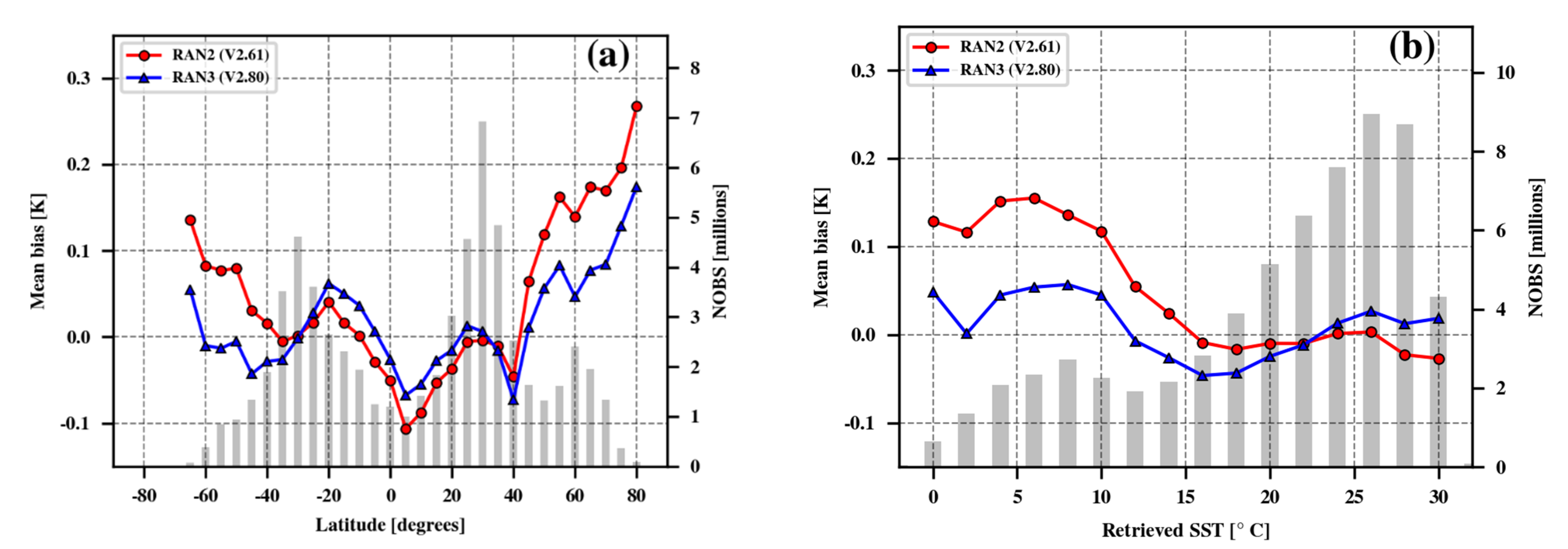
Validation of the RAN2 SSTs produced with V2.61, revealed ~+0.20 ± 0.05 K biases in the nighttime ‘subskin’ SSTs wrt (D+TM) SSTs at high latitudes (HL). Similar biases were also present in ‘depth’ SSTs, although with a reduced magnitude of ~+0.10 ± 0.03 K. Both SSTs were largely consistent between NPP and N20. Figure 2 shows RAN2 and RAN3 biases in ‘subskin’-(D+TM) SSTs, stratified by latitude and by satellite-retrieved ‘subskin’ SST. The RAN2 SST was biased warm at HL, and the bias plotted as a function of retrieved SST, appears near linear. In V2.80, it was empirically corrected by subtracting a linear HL correction term Δ_HL = a + b × (T − 273.15 K), where T is the retrieved SST in kelvins. Note that this correction is equivalent to multiplying all terms in the NLSST Equations (1) and (2) (except offset) by a single number, and then modifying the offsets accordingly. The correction can thus be implemented as new sets of the NLSST coefficients, without changing the form of the algorithm. We followed this procedure in ACSPO V2.80 and used NPP and N20 data from 2019 to compute the correction coefficients (a, b) for ‘subskin’ and ‘depth’ SSTs listed in

Table 3. Coefficients of the HL correction term, Δ_HL, for NPP and N20 ‘subskin’ and ‘depth’ SSTs. The ACSPO SSTs are obtained by adding Δ_HL to the NLSSTs calculated by Equations (1) and (2).

Satellite	a (K)	b (Unitless)
NPP (‘subskin’)	0.1420	−0.00650
N20 (‘subskin’)	0.1890	−0.00880
NPP (‘depth’)	0.0939	−0.00450
N20 (‘depth’)	0.0997	−0.00450

. The results shown in Figure 2 are produced from an independent 2020 ACSPO dataset, demonstrating that the bias in RAN3 has effectively flattened out as a function of SST, although some smaller residuals remain. Note that only the nighttime LUTs were modified using this procedure, because no systematic HL bias was observed in the daytime SSTs. The reason for the warm HL biases in RAN2 were likely the sparsity of in situ data at HLs, leading to the corresponding data being under-represented in the matchup dataset used for training the ACSPO V2.61. This under-representation in RAN2 was empirically corrected in RAN3.

Another improvement in ACSPO V2.80 was made to its clear-sky mask, ACSM, to reduce false-positive cloud detections in dynamic SST regions. The ACSM relies heavily on comparison of retrieved SST with the first-guess (L4 analysis) SST [1]. The L4 SSTs have much lower resolution than VIIRS L2/3 products (for instance, the CMC L4 employed in ACSPO, had 0.2° resolution prior to 31 December 2016 and 0.1° thereafter), and do not always capture position and strength of the SST gradients present in the L2/3 data (in dynamic formations such as eddies, cold upwellings etc). As a result, the cold side of the thermal fronts was often misclassified by the ACSM in V2.61 as cloud. The reliance on first-guess SST is reduced in V2.80, by replacing direct in-pixel L2 SST comparison with interpolated L4 SST, with checking against the minimum and maximum L4 SST values within a moving spatial window around the satellite pixel. In regions with uniform SST, the effect of this change on the ACSM is minimal. However, near thermal fronts, misclassifications of the cold side of the thermal fronts are now significantly reduced.

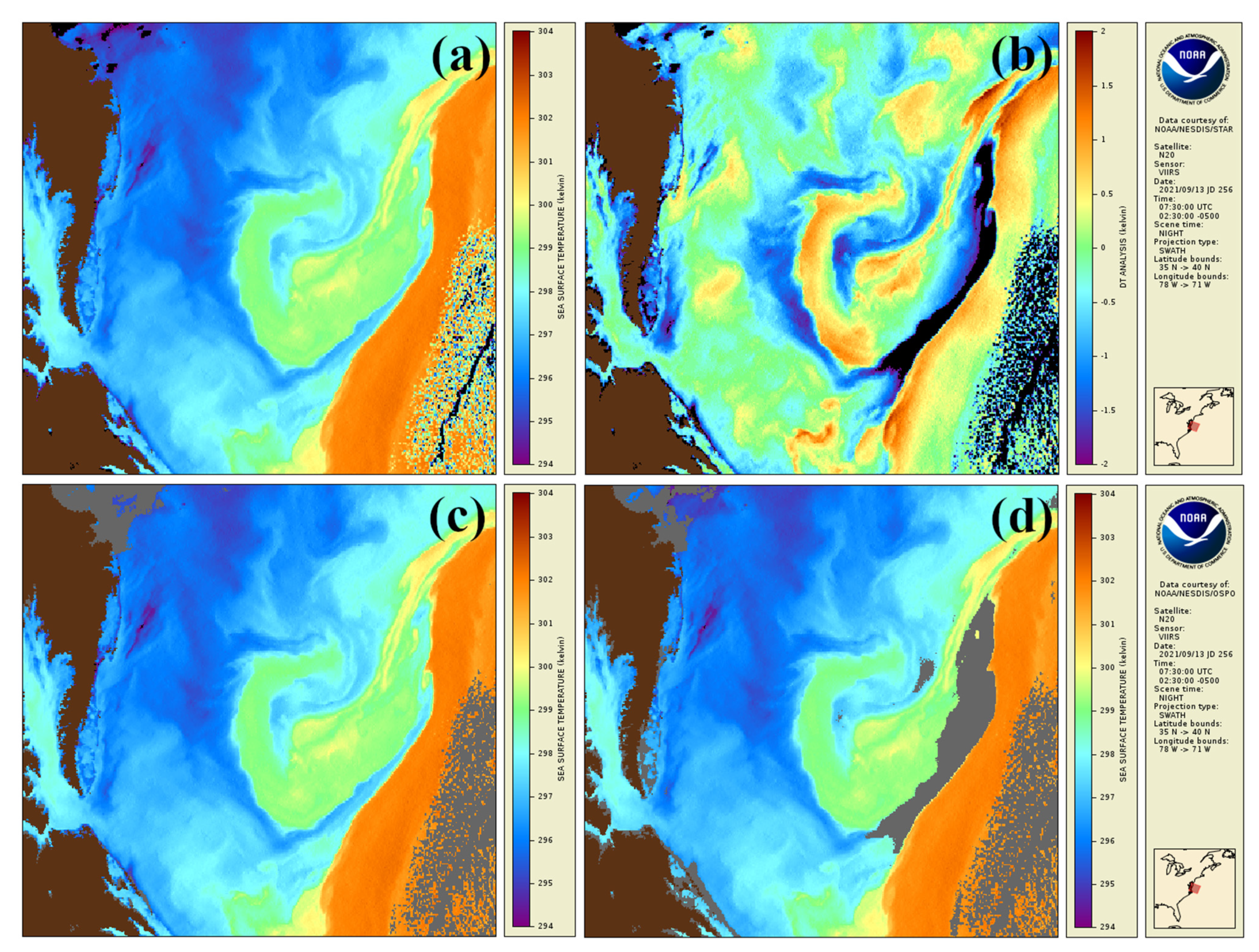
Figure 3 shows an example comparison of ACSPO V2.61 and V2.80 VIIRS L2P SST imagery in a dynamic region of Gulf Stream near Chesapeake Bay. Figure 3a shows ACSPO V2.80 SST without the clear-sky mask applied, and Figure 3b shows the corresponding delta between the satellite and first-guess SSTs. There is quite a bit of residual spatial structure in Figure 3b, because the feature resolution in the first-guess SST is lower and fails to capture the strong thermal fronts present in satellite data. The V2.80 mask shown in Figure 3c performs well near the thermal front, with no apparent over-screening, while the V2.61 mask (shown in Figure 3d) systematically over-screened the cold anomalies.

Another change in the V2.80 ACSM is in the BT test [1], where observed and CRTM simulated BTs are compared and pixels are marked as not clear, if the delta exceeds a set threshold. Simulated BTs are computed using CRTM V2.3.0, using NASA MERRA2 atmospheric profiles and today’s CMC L4 SST in DM and RAN, and NOAA GFS and yesterdays’ CMC L4 SST, in NRT production [37]. Stability of ΔBTs is monitored in the NOAA MICROS online system [38]. During the development of ACSPO V2.61, it was observed that the ACSM BT filter had triggered many false cloud detections. To mitigate its adverse effect, the ΔBT thresholds were set conservatively high. With such loose thresholds, the BT filter ended up having a very low specificity (i.e., the pixels, on which it was triggered, were already flagged by other clear-sky tests) and was subsequently disabled in ACSPO V2.70 and later versions. Due to the high BT filter thresholds set in ACSPO V2.61, the removal of the BT filter introduced only minor differences in the V2.80 ACSM.

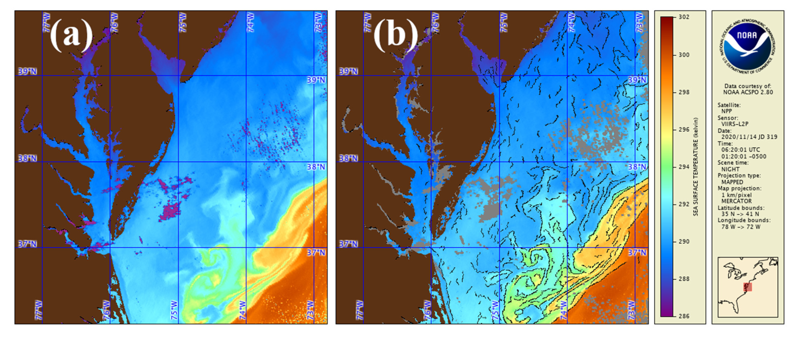
Thermal fronts are a new product first introduced in ACSPO V2.80. Information about thermal fronts is saved in ACSPO files in two new variables, the ‘sst_front_position’ and the ‘sst_gradient_magnitude’. The first variable is a binary indicator of SST front position in the valid SST clear-sky domain. It is set to ‘1’ where a front is present, and to ‘0’ elsewhere. The second variable is the SST gradient magnitude (in units of K/km), calculated from ‘subskin’ SST. The gradient magnitude is only reported in pixels where a front is present. Figure 4 shows example nighttime NPP ACSPO ‘subskin’ SST imagery over the Chesapeake Bay on 14 November 2020. SST imagery is shown without ACSM (Figure 4a), and with ACSM and with thermal fronts overlaid (Figure 4b). Black curves denote pixels where thermal fronts were detected. Figure 4 shows that the thermal fronts indeed accurately capture the positions of high SST gradients. Comprehensive evaluation and documentation of the new ACSPO thermal fronts product is beyond the scope of this work and will be reported elsewhere.

Note that image quality is critically important for frontal detection. Recall that similarly to MODIS, VIIRS is a multi-detector instrument. Each VIIRS across track scan contains 16 rows, for moderate resolution bands. The multi-detector design has a noticeable effect on imagery, which is more pronounced closer to the swath edge. The well-known consequence of this design is the bow-tie effect, where pixels from neighboring scans overlap. As pointed out by one of our reviewers, another imagery artifact is that pixels at a given distance from nadir do not follow a straight line in the along-track direction within a single scan (they make a slight angle relative to this line). Additionally, there is a discontinuity in the along-track direction between neighboring pixels from different scans. Starting with ACSPO V2.61, all VIIRS and MODIS L1b data go through an extra preprocessing step, where imagery is resampled to correct for artifacts resulting from their multi-detector design [23]. The main motivation for implementing the resampling algorithm in ACSPO was to facilitate the anticipated inclusion of thermal fronts in L2P imagery, as well as to improve the ACSPO clear-sky mask that uses spatial context information and, potentially in the future, pattern recognition algorithms [39].

3. Validation of ACSPO VIIRS SSTs against In Situ SSTs

In this section, NPP and N20 VIIRS ‘subskin’ and ‘depth’ SSTs are validated against in situ data from the NOAA iQuam online system [24,25]. The matchup criteria select all satellite pixels within 10 km × 30 min around an in situ measurement, forming a ‘one-to-many’ matchup data set (MDS), with each pair of in situ and satellite measurement considered an independent matchup. Note that only in situ data with the highest iQuam quality level, QL = 5, are used. The two main SST validation metrics are accuracy (global mean bias wrt quality controlled in situ SSTs) and precision (corresponding standard deviation, SD). The NOAA SST requirements are ±0.2 K for accuracy and 0.6 K for precision. Section 3.1 and Section 3.2 show that these requirements are met with a wide margin, when VIIRS SSTs are compared against drifters and tropical moorings (D+TM) as well as against fully independent Argo floats (AFs). Section 3.3 presents analysis of the long-term stability of ACSPO VIIRS SSTs. Note that this study focuses on L2P data. The performance of the L3U data is comparable with L2P and not analyzed here, in the interest of space.

3.1. Validation against Drifters and Tropical Moorings (D+TM)

Owing to a large number of drifters deployed worldwide, they represent the most valuable resource for calibration (training) and validation (independent assessment) of satellite SST products (often collectively referred to as ‘Cal/Val’). Up to 1500+ drifters have been operational in recent 10 years or so [25], providing SST measurements hourly (some platforms sample every 5 min) at a depth of ~20 cm. The shallower measurement depth (compared to ~1 m for the TMs and ~5 m for the AFs) makes drifters better suited for validating the satellite ‘subskin’ SSTs, especially under low wind and high solar insolation conditions. No other source of in situ SST data matches the number of measurements and the wide geographical distribution of drifters, including regions where in situ SST data are sparse (e.g., in the Arctic and Antarctic). Due to the lower number of drifters in equatorial regions, in ACSPO Cal/Val they are supplemented by the TMs [18], despite the facts that the TM measurements are taken somewhat deeper (~1 m) and are available from much fewer active platforms (between 25 and 100 during the recent decade) [25]. Figure 5 shows a typical yearly aggregate map of nighttime satellite matchups with (D+TM). Their coverage is near global, except in some limited regions with persistent clouds, heavy aerosols, or small number of (D+TM)’s (such as the west coast of Africa and South America, east coast of Argentina, waters around Indonesia, and the Gulf of Mexico).

Figure 6 shows the corresponding yearly aggregated histograms of ‘subskin’ and ‘depth’ ΔSSTs, during both daytime and nighttime.

All histograms are near Gaussian, without noticeable cold tails, indicating that the effect of cloud leakages is small. The daytime distributions (Figure 6c,d) are wider than nighttime (Figure 6a,b), for two reasons. First, the absence of the atmospherically transparent 3.7 µm band in the 3-band daytime SST algorithm given by Equation (1), leads to its degraded performance, compared to the 4-band nighttime algorithm given by Equation (2). Second, during the daytime, diurnal thermocline introduces additional differences between the skin (which IR sensors are sensitive to) and depth (at ~20 cm for drifters and ~1 m for the TMs) SSTs, which are larger than at night and more variable in space and time. The diurnal thermocline is close to its peak around 1:30 pm, when the afternoon NPP and N20 satellites overpass (cf. midmorning platforms, such as Metops, overpassing at 9:30 am). The histograms of ΔSST for the ‘depth’ SST are narrower than for ‘subskin’. This is expected due to the ACSPO ‘depth’ SST being a better proxy for SSTs at a depth close to that of (D+TM) measurements. Note that the yearly aggregated histograms in Figure 6 are based on ~63 million matchups and are therefore statistically representative (in addition to being globally representative; cf. Figure 5). The clear-sky domain (percent of clear-sky SST pixels to the total ice-free ocean pixels; not shown in Figure 6) is 18.4% for nighttime and 19.7% for daytime SSTs. The corresponding histograms and validation statistics for NPP (not shown) are consistent with the N20 results in Figure 6.

Figure 7 shows the time series of NPP, N20 and Aqua 24 h aggregated accuracy (global mean biases) and precision (SDs) of ACSPO nighttime SSTs wrt (D+TM).

NOAA requirements (±0.2 K for accuracy and 0.6 K for precision) are indicated by dashed lines. (Note that the Aqua SSTs produced with ACSPO system and presented in this work, are preliminary and only shown here to place VIIRS SST in historical MODIS perspective.) Typically, both NOAA requirements are met and often exceeded, by a wide margin. The NPP and N20 SSTs are very consistent for both ‘subskin’ and ‘depth’ SSTs. There is a ~0.05 K near constant offset between the NPP/N20 family, and the preliminary Aqua SSTs. (This bias can be easily adjusted by changing the offset in the Aqua NLSST retrieval equations, with revised SST retrieval coefficients. The iterations with the ACSPO Aqua MODIS dataset are currently underway, and it will be improved and reconciled with other ACSPO records, before public release.) Otherwise, the long-term trends in the respective biases are quite consistent across all three platforms. An interesting aspect of both nighttime ‘subskin’ and ‘depth’ SST biases is a systematic ~0.05 K cold ‘step’ prior to 2016, observed in both NPP and Aqua data against (D+TM)’s. However, it is not seen against AFs or TMs (see Section 3.2 and Section 3.3), suggesting a systematic warm bias in drifter SSTs prior to 2016. As expected, ACSPO ‘depth’ SSTs agree better with in situ data than the ‘subskin’ SST, with an improved precision (by 0.04–0.05 K margin). The SDs of the VIIRS and MODIS SSTs are only slightly reduced for VIIRS (by 0.01–0.02 K). The improvement in nighttime VIIRS SST precision is similar in magnitude to the improvements gained by adding the 8.6 µm band to the VIIRS NLSST given by Equation (2).

Figure 8 shows the corresponding daytime time series. The accuracy requirements are always met for ‘depth’ SST, and most of the time for ‘subskin’ SST. An expressed seasonal cycle (with a ~0.2 K amplitude for ‘subskin’ SST) may be attributed to regional and seasonal variations of the diurnal warming cycle in ΔSST = Satellite-(D+TM) SSTs, as Sun illumination systematically progresses from one hemisphere to the other. The amplitude of the seasonal variations is significantly reduced in magnitude (~0.1 K) for ‘depth’ SSTs, suggesting that the ACSPO PWR algorithm successfully reconciles satellite SST with in situ (D+TM) SSTs, in which the diurnal cycle is suppressed. NPP and N20 global mean biases remain very consistent, with no noticeable systematic or time-dependent differences. However, both platforms show a drift of approximately −0.1 K/decade, whereas MODIS-Aqua daytime SSTs are more stable in time. More quantitative estimates of SST stability are presented in Section 3.3. Figure 8c,d show that precision of ‘depth’ SST is significantly improved compared to ‘subskin’ SST, with about 0.08–0.09 K margin for all three platforms. The daytime precision of VIIRS SST is improved compared to MODIS, by 0.04–0.06 K for both ‘subskin’ and ‘depth’ SSTs. The wider margin, compared to nighttime SSTs (0.01–0.02 K), may be attributed to the availability of the VIIRS 8.6 µm band, which has a larger impact during daytime and leads to improved retrievals, compared to MODIS SSTs produced with only two LWIR bands, 11 and 12 µm.

3.2. Validation against Argo Floats (AFs)

The Argo program commenced in 1999, reached its target of ~3000 active floats in 2008 [40,41] and grew to 3500+ after 2012 [25]. The AFs are different from drifters and tropical moorings in that they measure vertical profiles of sea temperature and salinity at depths ranging from typically 4–5 m to 2 km, on a 10-day cycle. Most AFs do not measure sea temperature above 4–5 m. However, some floats deployed after 2013 carry a secondary sensor capable of near-surface measurements at depths as shallow as 20 cm [42]. Despite twice as many AF platforms as (D+TM)’s, they provide two orders of magnitude fewer SST observations, because they spend most of their time deep in the ocean, only surfacing every 10 days. Despite their relative sparsity compared to (D+TM)’s, AFs are extremely valuable for validation of satellite SSTs, serving as an independent reference (which is not used for training, or ‘calibration’ of ACSPO SST algorithms).

Figure 9 shows an example of yearly aggregated maps of VIIRS nighttime ‘subskin’—AFs ΔSSTs. Geographical coverage by AFs matchups is generally globally representative but much sparser compared to (D+TM)’s (cf. Figure 5).

Figure 10 shows corresponding histograms of ‘subskin’—AF and ‘depth’—AFs ΔSSTs (cf. ΔSSTs wrt (D+TM)s in Figure 6). At night, the histograms of both ΔSSTs are Gaussian, and slightly narrower (0.01 K smaller SDs) compared to the corresponding (D+TM) histograms. During the daytime, both ‘subskin’ and ‘depth’ histograms are biased slightly warm and have warmer tails than wrt (D+TM)’s (cf. skewness in Figure 6 and Figure 10). Both effects are due to the deeper measurement depths for AFs than for (D+TM)’s. The daytime histograms are also significantly wider (higher SDs) because of stronger and more variable diurnal warming (see discussion in Section 3.1). The yearly aggregated AF histograms are based on ~0.7 million matchups (cf. 62–63 million matchups with D+TM). Figure 5 and Figure 9 show that albeit two orders of magnitude sparser than (D+TM), the AF matchups are globally representative. The corresponding histograms and validation statistics for NPP (not shown) are consistent with the N20 results in Figure 10.

Figure 11 shows time series of ACSPO nighttime validation statistics for NPP, N20 and Aqua wrt AFs. The results are now aggregated monthly due to the much smaller number of AF matchups compared to the (D+TM). NOAA requirements for accuracy and precision continue to be met and exceeded by a wide margin. The NPP and N20 SSTs remained very consistent, with no apparent systematic trends in either ‘subskin’ or ‘depth’ SSTs. The mean AF biases in Figure 11 agree with the corresponding (D+TM) biases in Figure 7, except that there is no ~0.05 K ‘step’ in 2016 in the AF ΔSSTs. This suggests that the issue is likely with the (D+TM) SSTs and not with the satellite SSTs. Aqua remains in-family with NPP and N20, except that there is the same ~+0.05 K bias due to the untuned NLSST offset in the initial ACSPO MODIS implementation. The VIIRS nighttime precision slightly outperforms MODIS (by ~0.02 K for both ‘subskin’ and ‘depth’ SSTs), consistent with the (D+TM) results in Figure 7. Again, ‘depth’ SSTs agree better with the AFs than do ‘subskin’ SSTs, with a 0.03 K improvement margin (consistently with the (D+TM) validation in Figure 7).

Figure 12 shows the corresponding daytime validation statistics versus AFs.

Due to the AF’s ~5 m depth, their corresponding daytime ΔSSTs are subject to stronger diurnal thermocline, compared with the (D+TM) statistics in Figure 8. All NPP, N20 and Aqua AF ΔSSTs are biased warm by ~+0.2 K, compared to the corresponding (D+TM) ΔSSTs. After mid-2019, an unexplained ~−0.1 K ‘step’ and increased noise are observed. Consistency across all satellite sensors suggests that it likely comes from the AF data itself. The fact that the ‘step’ and increased noise are not immediately observed at night (cf. Figure 11a,b), may suggest that an increased number of near-surface (shallower than ~5 m) AF measurements may be a contributing factor. Comparison of Figure 8c,d and Figure 12c,d shows that the daytime SDs wrt AFs increases compared to (D+TM) SDs for both ‘subskin’ and ‘depth’ SSTs. This is expected, due to the larger diurnal thermocline signal in AF ΔSSTs, which depends on the wind speed and solar insolation and is highly variable in space and time. More analyses are needed to fully understand and reconcile the AF and (D+TM) validation results.

3.3. Long-Term SST Stability

While more numerous and geographically representative, drifters may be less accurate than the TMs (see [43] and references within). Additionally, the geographical distribution of drifters is less stable in time, making it difficult to separate artifacts in satellite SSTs from those caused by regional and seasonal biases in the in situ network. The improved stability of the TM SSTs, in conjunction with their more stable geographical domain and reduced seasonal SST cycle in the tropics, lends itself to studies of long-term stability of satellite SSTs. The high atmospheric water vapor content in the tropics means that more atmospheric correction is applied in the NLSST equation than for drier higher-latitude atmospheres, making SST retrievals more sensitive to calibration drifts in all employed thermal bands. For this reason, comparisons with the TMs are expected to provide a more stringent test for stability of satellite SSTs. Note that previously, TMs were used to estimate stability of satellite SSTs produced by the (A)ATSR Reprocessing for Climate (ARC) project [44]. This section explores TMs to estimate the relative stability of the NPP/N20 VIIRS and Aqua MODIS ACSPO SST retrievals.

Figure 13 shows time series of ACSPO global mean biases for NPP, N20 and Aqua ΔSST wrt TMs. As with AFs, the results are aggregated monthly, due to the ×20 smaller number of TMs compared to drifters. For each time series, the slope (calculated using a linear least square fit) in units of K/decade is given, along with the associated uncertainty obtained from a 95% confidence interval.

Figure 13a,b show that nighttime NPP SSTs are very stable, with small and statistically insignificant drifts of (−0.011 ± 0.013) and (−0.008 ± 0.011) K/decade for ‘subskin’ and ‘depth’ SSTs, respectively. Aqua SSTs shows minor drifts of (+0.026 ± 0.016) K/decade for ‘subskin’ and (+0.012 ± 0.012) K/decade for ‘depth’ SSTs. N20 SSTs drift with a rate of (−0.066 ± 0.049) K/decade for ‘subskin’ and (−0.045 ± 0.062) K/decade for ‘depth’ SSTs. The shorter N20 mission (only 4 years) results in larger uncertainties. Overall, considering their corresponding uncertainties, all three drifts are essentially close to zero.

Figure 13c,d show the corresponding daytime results. They are much noisier than at night, due to the strong diurnal thermocline present in the tropics at 1:30 pm local time. Statistically significant negative drifts are seen in the NPP data, (−0.136 ± 0.038) K/decade for ‘subskin’ and (−0.080 ± 0.025) K/decade for ‘depth’ SSTs. The N20 drifts, (−0.251 ± 0.157) K/decade for ‘subskin’ and (−0.184 ± 0.115) K/decade for ‘depth’ SST, are higher and more uncertain, due to its shorter mission. However, within their uncertainties, the NPP and N20 slopes are statistically indistinguishable. Out of all three satellites, Aqua shows the smallest trends, (+0.015 ± 0.042) K/decade for ‘subskin’ and (+0.036 ± 0.025) K/decade for ‘depth’ SST. Both are effectively zero, given their uncertainties.

The major observations from Figure 13 are that drifts in the nighttime VIIRS and MODIS ΔSSTs are largely consistent and close to zero, whereas in the daytime ΔSSTs, they are consistent and essentially negative (from −0.1 to −0.2 K/decade) for both VIIRSs, while for MODIS-Aqua, they are near zero.

Another way to estimate stability of satellite SSTs is to analyze ‘day minus night’ double differences (DDs) of ACSPO ΔSSTs wrt some common references (e.g., L4, D+TM or AFs SSTs). In the DDs, the biases and instabilities in the reference SSTs (for instance, a positive ~0.05 K ‘step’ prior to 2016 in drifter SST, cf. Section 3.1, and possible instabilities in the CMC L4 SST), cancel out, so that trends in the DDs characterize the relative consistency of daytime and nighttime satellite SSTs. All our analyses so far suggest that the nighttime trends from both VIIRSs and MODIS-Aqua are close to zero and consistent, making the day-night DDs an additional way to quantify the stability of daytime SSTs. Matchups with two references, (D+TM) and CMC L4, were analyzed. Figure 14 shows time series of monthly aggregated DDs calculated from daytime and nighttime (ACSPO—Reference) ΔSSTs, for two reference SSTs, (D+TM) and CMC L4 SST.

Note that the seasonal signal in the DDs was removed using the STL (Seasonal and Trend decomposition using Loess) algorithm [45] implemented from the ‘statsmodels’ python package [46]. The trends in the (D+TM) DDs shown in Figure 14a,b, look qualitatively similar to the daytime results against TMs in Figure 13c,d. However, the noise in the time series is significantly reduced, due to the shallower drifter measurement depth (~20 cm), increased matchup statistics (recall that there are ×20 more (D+TM)s compared to the TMs), additional STL de-seasoning [45], and calculation of DDs (which cancels noise in reference SST). The noise is further reduced in the L4 DDs shown in Figure 14c,d, due to at least four orders of magnitude more matchups with L4 compared to (D+TM)’s.

Estimates of nighttime and daytime trends are summarized in

Table 4. Drift in ACSPO ΔSSTs (K/decade) and associated uncertainties corresponding to a 95% confidence interval. Nighttime drifts are obtained via comparison to TMs presented in Figure 13a,b. The daytime results are calculated from day-night DDs of ACSPO—Reference ΔSSTs, where Reference = (D+TM) (Figure 14a,b) or L4 CMC SST (Figure 14c,d).

SST	NPP	N20	Aqua
Day ‘subskin’ (D+TM)	−0.143 ± 0.015	−0.115 ± 0.069	+0.013 ± 0.014
Day ‘depth’ (D+TM)	−0.078 ± 0.007	−0.058 ± 0.018	+0.006 ± 0.011
Day ‘subskin’ (L4)	−0.123 ± 0.013	−0.158 ± 0.053	+0.061 ± 0.012
Day ‘depth’ (L4)	−0.068 ± 0.007	−0.081 ± 0.021	+0.031 ± 0.010
Night ‘subskin’	−0.011 ± 0.013	−0.066 ± 0.049	+0.026 ± 0.015
Night ‘depth’	−0.008 ± 0.011	−0.045 ± 0.062	+0.012 ± 0.012

. The nighttime results are from comparisons with TMs in Figure 13a,b, whereas the daytime results are from the DD analyses in Figure 14. For example, the NPP daytime ‘subskin’-(D+TM) ΔSSTs drift at a rate of (−0.143 ± 0.015) K/decade, compared with Aqua (+0.013 ± 0.014) K/decade. The corresponding trends in ‘depth’ SSTs have the same signs, but about half the magnitude. The N20 daytime trends are more uncertain than NPP, due to its shorter mission of ~4 years. Interestingly, all NPP and N20 trends (for day/night and ‘subskin’/‘depth’ SSTs) overlap with a 95% confidence, suggesting that the two VIIRSs drift in-sync. The MODIS trends, if present, tend to be slightly positive. In any case, they are much closer to zero than the VIIRSs trends. Qualitatively, the DDs calculated with two different references, are largely consistent. Small quantitative differences may be due to different domains covered by day and night retrievals (especially in the high latitudes, where in situ day/night matchups are highly seasonal, in situ data are often missing and quality of satellite retrievals may be degraded and challenging to verify). More analyses are needed to understand and reconcile these quantitative differences. In any case, Table 4 clearly shows negative trends in daytime VIIRS SSTs of approximately −0.1 K/decade, whereas the MODIS trends, if exist, are slightly positive and much closer to zero.

Note that ACSPO VIIRS and MODIS algorithms use consistent clear-sky mask and SST equations (except that the 8.6 µm band is not used for MODIS), and identical ancillary data (first-guess SST and atmospheric profiles). This means that the most probable cause for the observed drift in the VIIRS daytime SSTs (which is surprisingly consistent across two sensors) was degradation of the VIIRS BTs. The stability of the VIIRS and MODIS BTs is analyzed in the next section.

4. Stability of VIIRS BTs

In ACSPO, modeled BTs are simulated using the Community Radiative Transfer Model (CRTM; current version v2.3.0). The NOAA Monitoring of Infrared Clear-sky Radiances over Ocean for SST (MICROS) online system [26,27,38] calculates observed (O) minus modeled (M) BT differences (ΔBTs, or ‘O-M’ biases) and monitors their stability in time. MICROS is an essential component of the NOAA SST monitoring and represents a valuable resource to trace root causes of any problems with stability of the retrieved SSTs, due to any changes in sensor BTs. Special care must be taken to separate any biases introduced by the ‘O’ and ‘M’ terms. This is particularly important when analyzing gradual subtle multi-year calibration degradations of 0.1 K/decade or less. The input sources for the ACSPO implementation of the CRTM forward model are CMC L4 SST [37,47] and MERRA2 atmospheric vertical profiles of pressure, temperature and humidity [48] (in the near-real-time mode, GFS forecast is used instead [49]). Effects of model-induced biases are mitigated by calculating DDs of the O-M biases between different sensors. As in case of SST DDs, the O-M BT DDs only give relative stability between different sensors and are most valuable when a known stable sensor’s BTs are available. However, even in the absence of a known stable sensor, BT DDs can be correlated with trends in satellite SSTs discussed in Section 3.3.

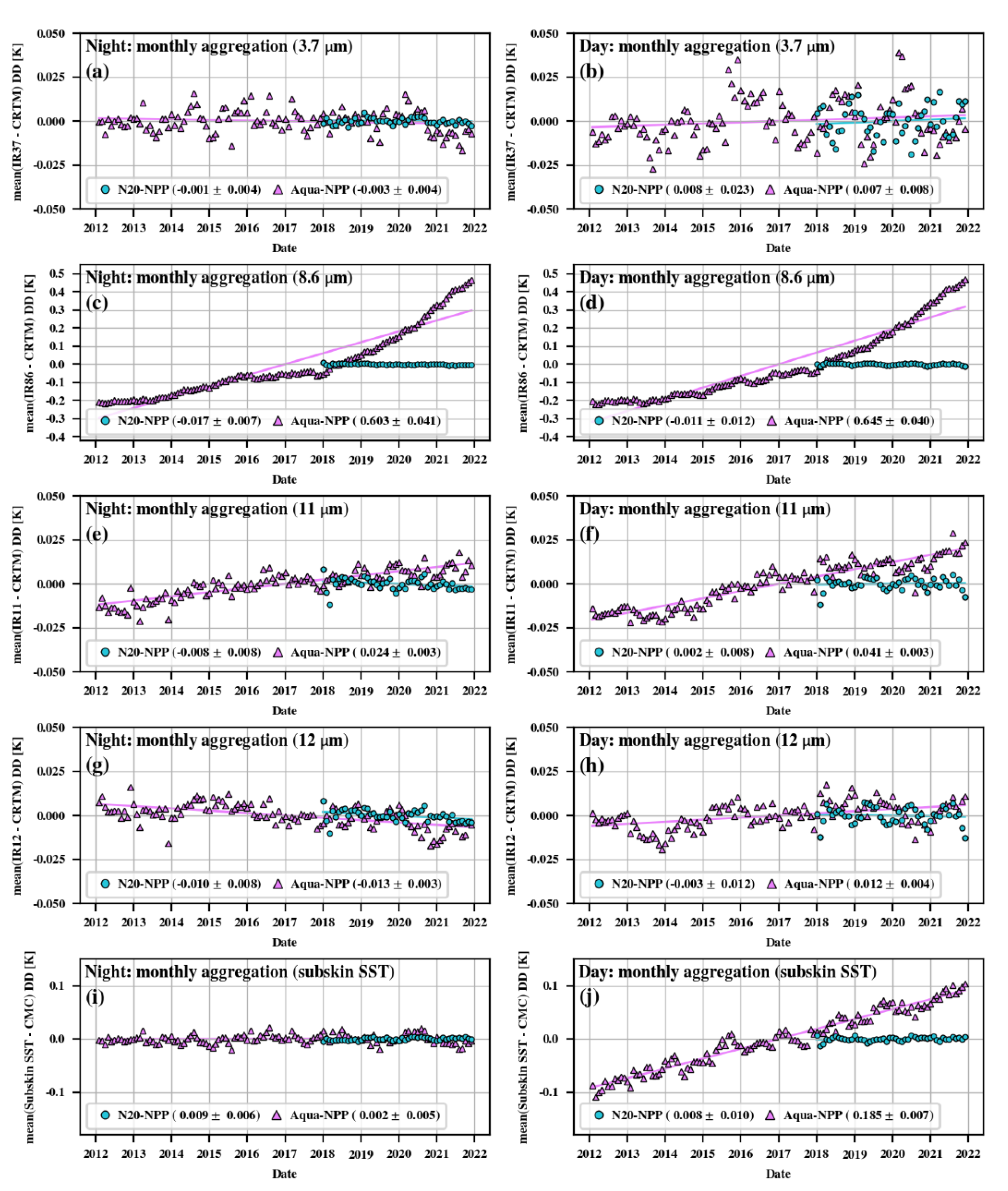
Long-term stability of BTs is analyzed by comparing O-M biases between VIIRS sensors onboard NPP/N20 and MODIS-Aqua. MODIS and VIIRS have similar bands, and Aqua flies in a similar orbit with LEXT ~1:30 am/pm. Figure 15 shows monthly aggregated O-M DDs for the bands centered at 3.7, 8.6, 11 and 12 µm, separately for day and night.

All DDs are calculated wrt NPP (i.e., the NPP O-M is always subtracted). The seasonal signal in the Aqua—NPP DDs (e.g., due to differences between VIIRS and MODIS spectral response functions which may have not been fully accounted in the CRTM calculations) has been removed using the STL algorithm [45]. For the N20—NPP DDs, no measurable seasonal signal was detected (likely to their closer spectral response functions) and no seasonal detrending was needed. For each band and satellite, the temporally averaged ‘mean DD’ (approximately 0.1 K) was subtracted, to center all of the time series at 0 K and aid in visualization of the trends. Non-zero mean DDs may be again due to e.g., small differences in spectral response functions unaccounted for in CRTM. Systematics biases in BTs are not critical for SST retrievals with the empirically tuned NLSST Equations (1) and (2) (they can be absorbed by, for example, adjusting the NLSST offset). Our objective was to evaluate temporal stability of the O-M DDs, not their mean values. For each time series the slope (K/decade, obtained using a linear least square fit) is given, along with its associated uncertainty obtained using a 95% confidence interval.

Figure 15a shows that nighttime BTs in the 3.7 µm band are stable, on all three satellites. This is indirectly suggested by the near-zero trends in both DDs (N20—NPP and Aqua—NPP), well within their uncertainties. Stability of the 3.7 µm band is crucial for accurate nighttime SST retrievals, when it is the dominant contributor to SST (cf. Table 1). The consistency of MODIS and VIIRS 3.7 µm bands results in excellent stability and inter-sensor consistency of ACSPO nighttime SSTs (cf. Section 3.3). (During the daytime, the 3.7 µm band is not used for SST retrievals, but it is included in Figure 15b for completeness. No statistically significant trends are seen during the daytime either, although uncertainties are much higher due to the contribution of reflected solar radiation to the 3.7 µm BTs.)

The 8.6 µm band is an outlier on MODIS-Aqua, showing a large increasing trend compared to NPP during both night (Figure 15c) and day (Figure 15d), while NPP and N20 are very consistent with each other, with a relative trend of (−0.017 ± 0.007) K/decade at night and (−0.011 ± 0.012) K/decade during the daytime. The 8.6 µm MODIS band 29 is not used in ACSPO SST retrievals, due to its unstable behavior. The bulk of the contribution of the Aqua—NPP 8.6 µm trend most likely comes from MODIS calibration degradation. The 0.6 K/decade drift in the VIIRS 8.6 µm band would (according to Table 1 and Table 2) result in a −0.08 and +0.45 K/decade drift in nighttime and daytime SSTs, respectively. This is much larger than observed in Figure 15i,j (and in the SST stability analyses in Section 3.3). The exact reason for the MODIS 8.6 µm unstable behavior is unknown, but this band has large electronic crosstalk [32]. The AVHRR instruments have no 8.6 µm band; thus, no independent validation of NPP stability was possible before N20 was launched and its thermal bands started transmitting high quality BTs on 5 January 2018. The NPP and N20 BTs in the 8.6 µm band are very consistent, which does not necessarily mean that they are stable. Future ACSPO reprocessing of ABI/AHI sensors (both have bands centered near 8.6 µm) flown onboard GOES-R and Himawari geostationary satellites, could extend independent sensor validation back to the 2015 when Himawari-8 data became available.

The BTs in the 11 µm band are very consistent between NPP and N20, with trends of (−0.008 ± 0.008) and (+0.002 ± 0.008) K/decade during night (Figure 15e) and day (Figure 15f), respectively. However, statistically significant trends are seen in Aqua—NPP DDs, on the order of (+0.024 ± 0.003) K/decade at night and (+0.041 ± 0.003) K/decade during the day. The trend in the NPP 11 µm band was estimated in [50] to be −0.02 K/decade, based on comparison of VIIRS BTs with the Cross-Track Infrared Sounder (CrIS) onboard the same NPP spacecraft (using both daytime and nighttime near-nadir BTs from March 2012–February 2017). Our estimates have the same sign as in [50] but are somewhat larger in magnitude, on average.

For the 12 µm band, N20—NPP DDs trends are (−0.010 ± 0.008) K/decade at night (Figure 15g) and (−0.003 ± 0.012) K/decade during the daytime (Figure 15h). Both are statistically insignificant. The trends in Aqua—NPP DDs are (−0.013 ± 0.003) K/decade at night and (+0.012 ± 0.004) K/decade during the daytime. They are statistically significant but counter-directed, and in any case smaller than in the 11 µm band. In [50], the authors also found a negative trend (compared to CrIS) of −0.02 K/decade in the NPP VIIRS 12 µm band, again based on a combination of near-nadir daytime and nighttime data. Such large trend is not supported by our analyses. Unfortunately, comparison with CrIS is not possible for the VIIRS 3.7 and 8.6 µm bands due to the limited spectral coverage of the CrIS instrument.

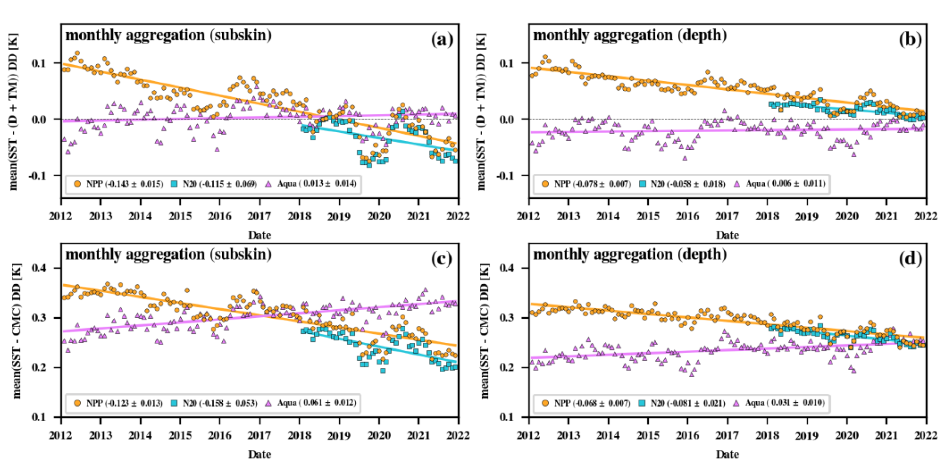
Figure 15i,j also show O-M DDs for SST, with ‘O’ = satellite ‘subskin’ and ‘M’ = CMC L4 SST [37,47]. The VIIRS and MODIS nighttime ‘subskin’ SSTs are very consistent, with trends <0.015 K/decade in N20—NPP DDs and <0.007 K/decade in Aqua—NPP DDs. As discussed above, this excellent agreement is not surprising, given the good stability of the NPP/N20 VIIRS and Aqua MODIS 3.7 µm bands. However, for daytime we found a +0.185 ± 0.007 K/decade bias drift of Aqua—NPP ‘subskin’ SST DD, while N20 and NPP are very consistent (<0.018 K/decade). Based on the close agreement between the two VIIRSs, it is tempting to conclude that the problem lies with MODIS-Aqua calibration. However, in Section 3.3 we demonstrated that NPP and N20 daytime SST biases wrt in situ SST have negative drifts (approximately (−0.143 ± 0.015) K/decade for NPP), while the Aqua MODIS daytime SST is much more stable, with statistically insignificant drift of (+0.013 ± 0.014) K/decade. Based on a daytime SST contribution of NPP VIIRS 11 µm band (2.886) and 12 µm band (−2.562) from Table 2, and their corresponding daytime Aqua—NPP trends of +0.041 and +0.012 K/decade in Figure 15, one would expect an NPP SST trend of ~−0.09 K/decade. This is not enough to account for the observed ~−0.14 K/decade NPP VIIRS daytime SST bias drift, unless also accompanied by a −0.08 K/decade drift in the NPP 8.6 µm band (based on its +0.757 weight contribution to daytime SST; see Table 2). Note that when producing these estimates, we have considered Aqua MODIS BTs as a trusted standard, motivated by its excellent SST temporal stability demonstrated in Section 3.3. However, the stability of the 8.6 µm band cannot be verified independently. As of this writing, we are not aware of any studies quantifying the stability of the VIIRS 8.6 µm band, with uncertainty sufficient for its use in SST stability analysis. The stability of this band can be (indirectly) verified by applying empirical corrections to VIIRS BTs and reprocessing SST from both NPP and N20 missions. Another option is to compare VIIRS BTs with AHI (flown onboard Himawari-8) or ABI (onboard GOES-R) 8.6 µm bands. Such a detailed investigation of VIIRS thermal band stability and mitigation of its daytime SST biases will be considered in the future.

5. Conclusions

Full-mission global SST records from 750 m resolution VIIRS data onboard two JPSS series satellites, NPP (1 February 2012—on) and N20 (5 January 2018—on), were produced using the NOAA Advanced Clear Sky Processor for Ocean (ACSPO) enterprise SST system version 2.80. This dataset is the 3rd historical reprocessing (Reanalysis-3, RAN3) of ACSPO VIIRS SST data going back to the beginning of both NPP and N20 missions. The RAN3 L2P and L3U data are archived at NASA/JPL PO.DAAC [7,8,9,10], and NOAA CoastWatch (complete L3U archive; L2P is available for the most recent two weeks only) [16]. New data are added in near real time (NRT) with a latency of a few hours. Delayed mode (DM) science-quality reprocessing lags NRT processing by two months, replacing NRT files with more complete and uniform, science quality DM data. Once a new ACSPO version is released, the next full-mission reanalysis will be undertaken.

For users interested in reduced data volume, we recommend the ACSPO L3S-LEO-PM product, which is an 0.02° gridded super-collated (L3S) product from afternoon (PM) low Earth orbiting (LEO) satellites [13,14,15,17,51]. L3S-LEO-PM currently includes data from both VIIRSs onboard NPP and N20. We plan to include MODIS-Aqua and future VIIRSs onboard JPSS-2/3/4 satellites in L3S-LEO-PM, when these data become available. An analogous mid-morning L3S-LEO-AM product is also available from AVHRR FRAC instruments flown onboard Metop-FG satellites (Metop-A/B/C) [5,17,52]. We plan to add SSTs from MODIS-Terra and METimage (to be flown onboard Metop-SG series satellites) to L3S-LEO-AM, when their ACSPO products become available. Currently, ACSPO RAN is the only complete record from both VIIRS instruments. Note that two other VIIRS SST datasets are produced by NASA JPL (full mission NPP; no N20 data available) [33,34] and NAVO (NPP data available back to 2013, with various periods processed by three different versions of the code; no N20 SST data are available) [35,36,53,54].

We described the ACSPO algorithm with emphasis on the improvements made while transitioning from RAN2 (produced with ACSPO V2.61) to RAN3 (produced with ACSPO V2.80). RAN3 also added N20 data. Algorithm improvements in RAN3 include mitigation of warm biases at high latitudes and reduction of false cloud detections in dynamic regions, where the cold side of thermal fronts was often misidentified as cloud in RAN2. ACSPO V2.80 also includes a new thermal fronts product, which provides information about presence and intensity of thermal fronts. Technical improvements include reduction of GDS2 L2P data size from ~10 to ~2.5 TB/year/sensor, accomplished by removing brightness temperature layers, increasing compression level and setting physically unrealistic SSTs to fill values.

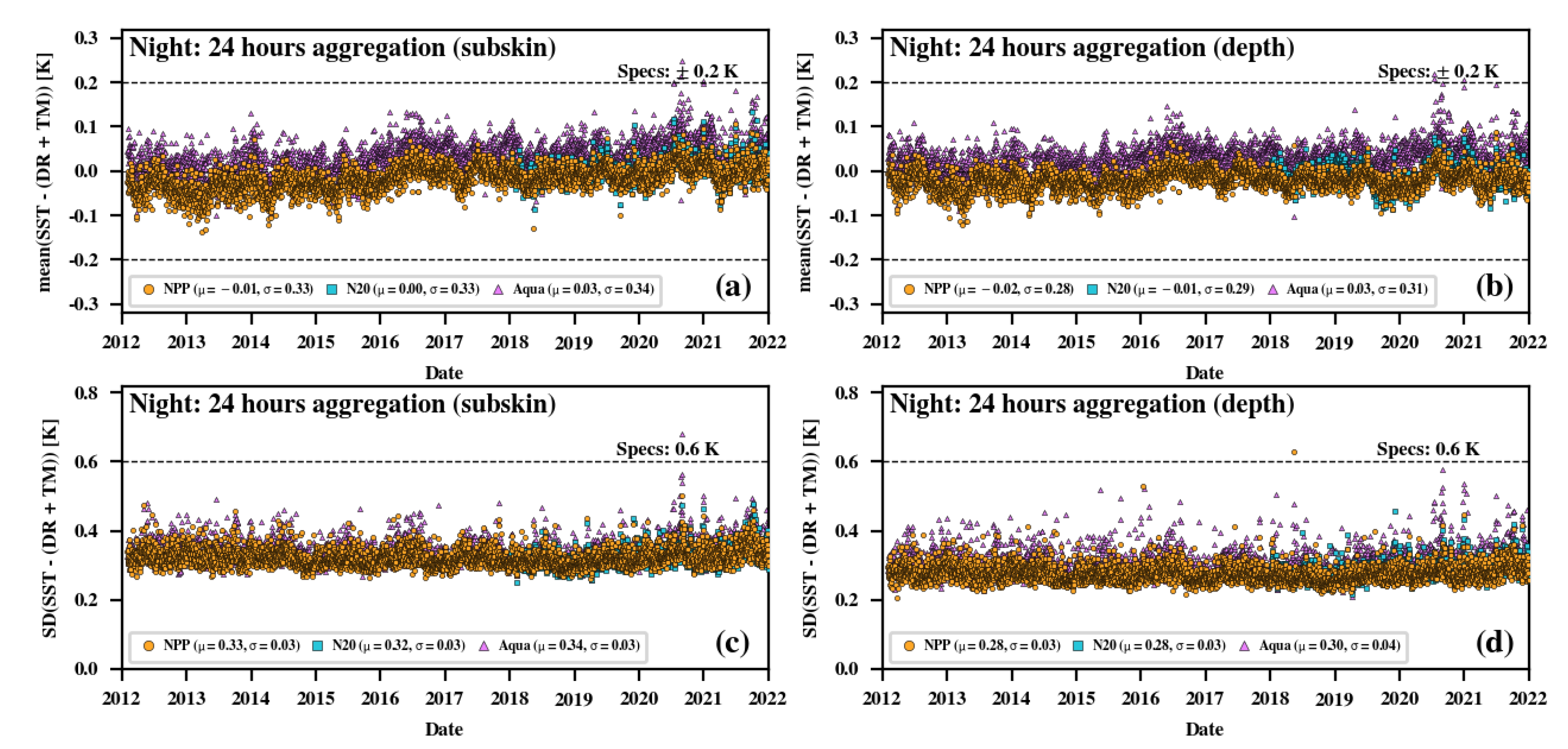
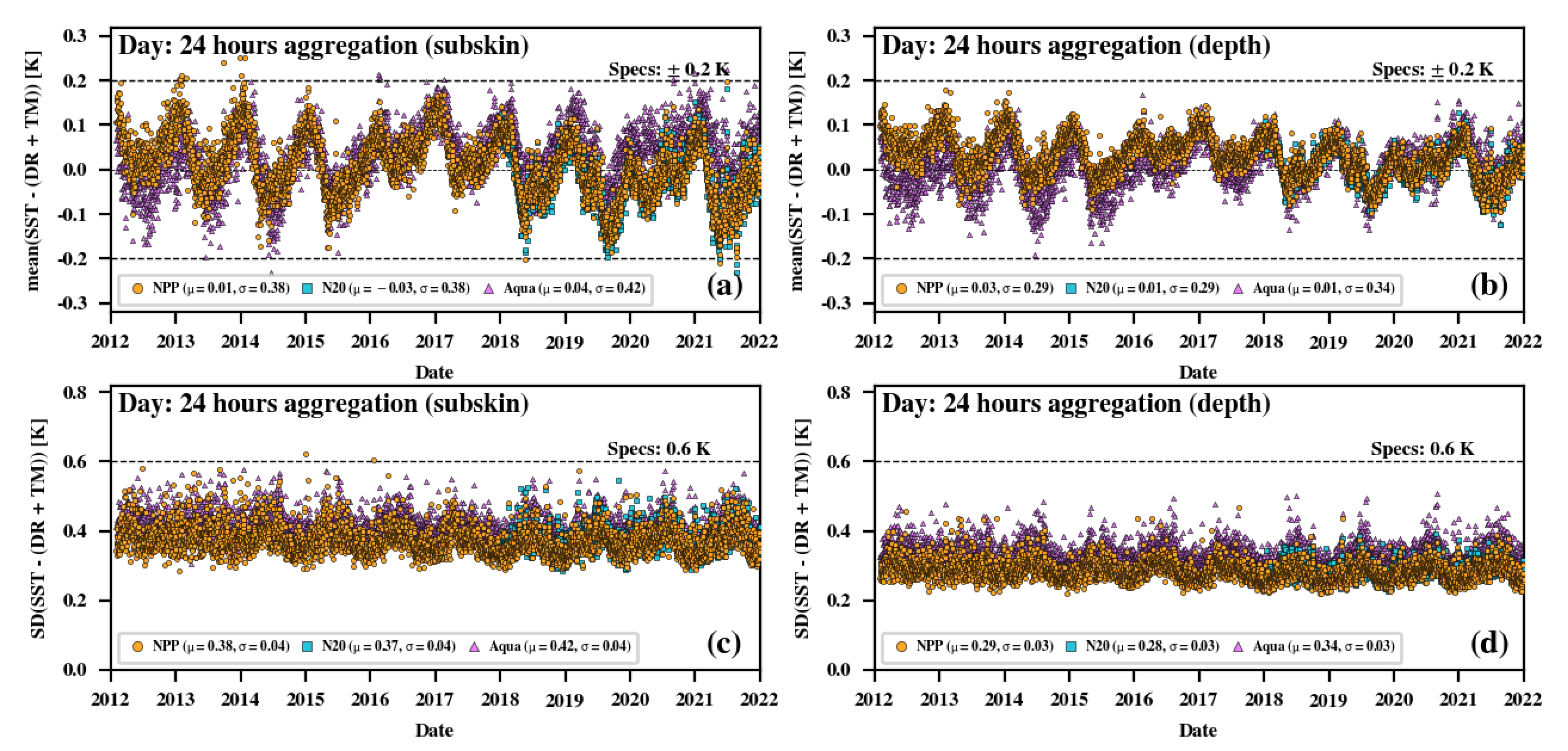
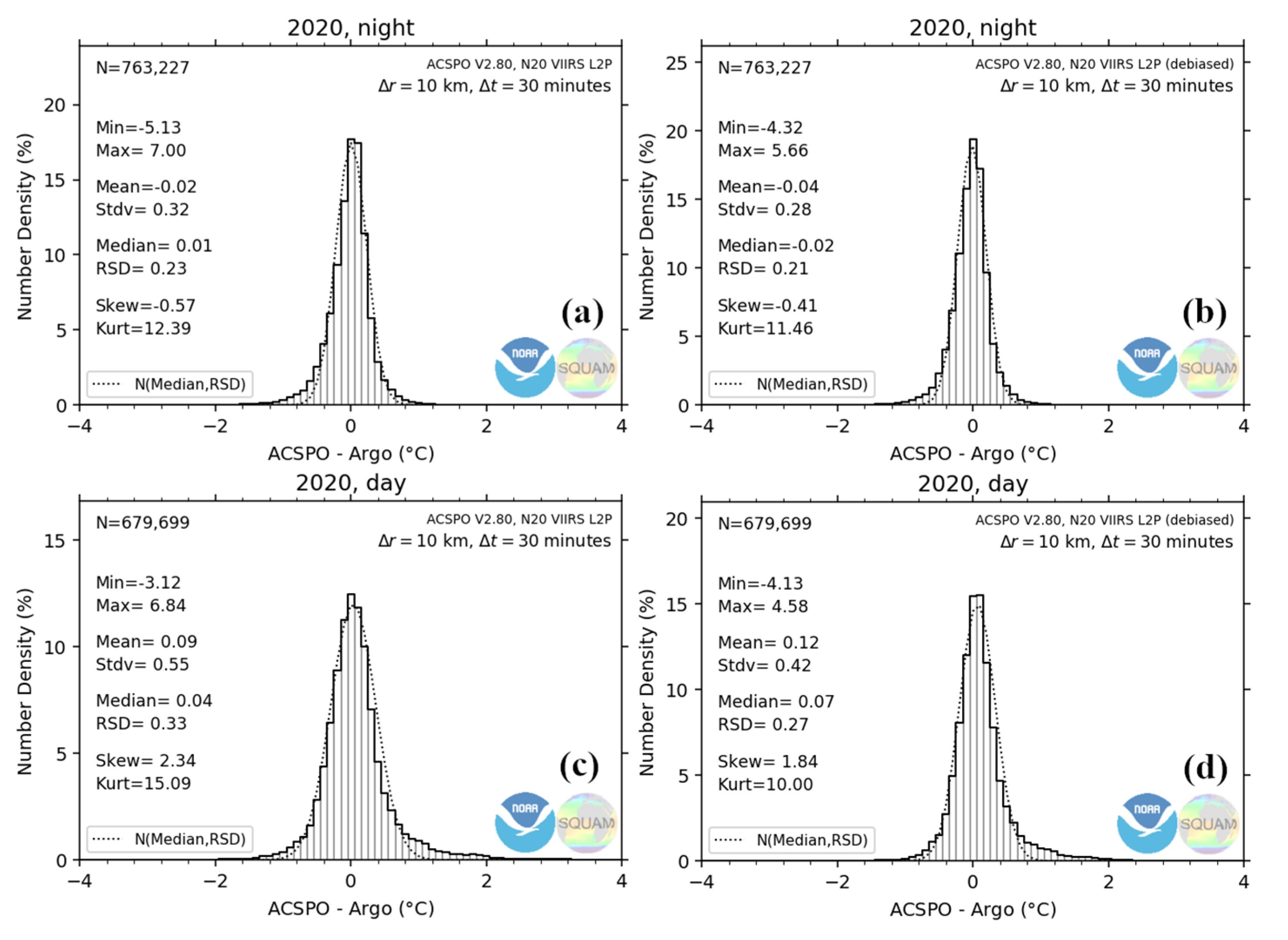
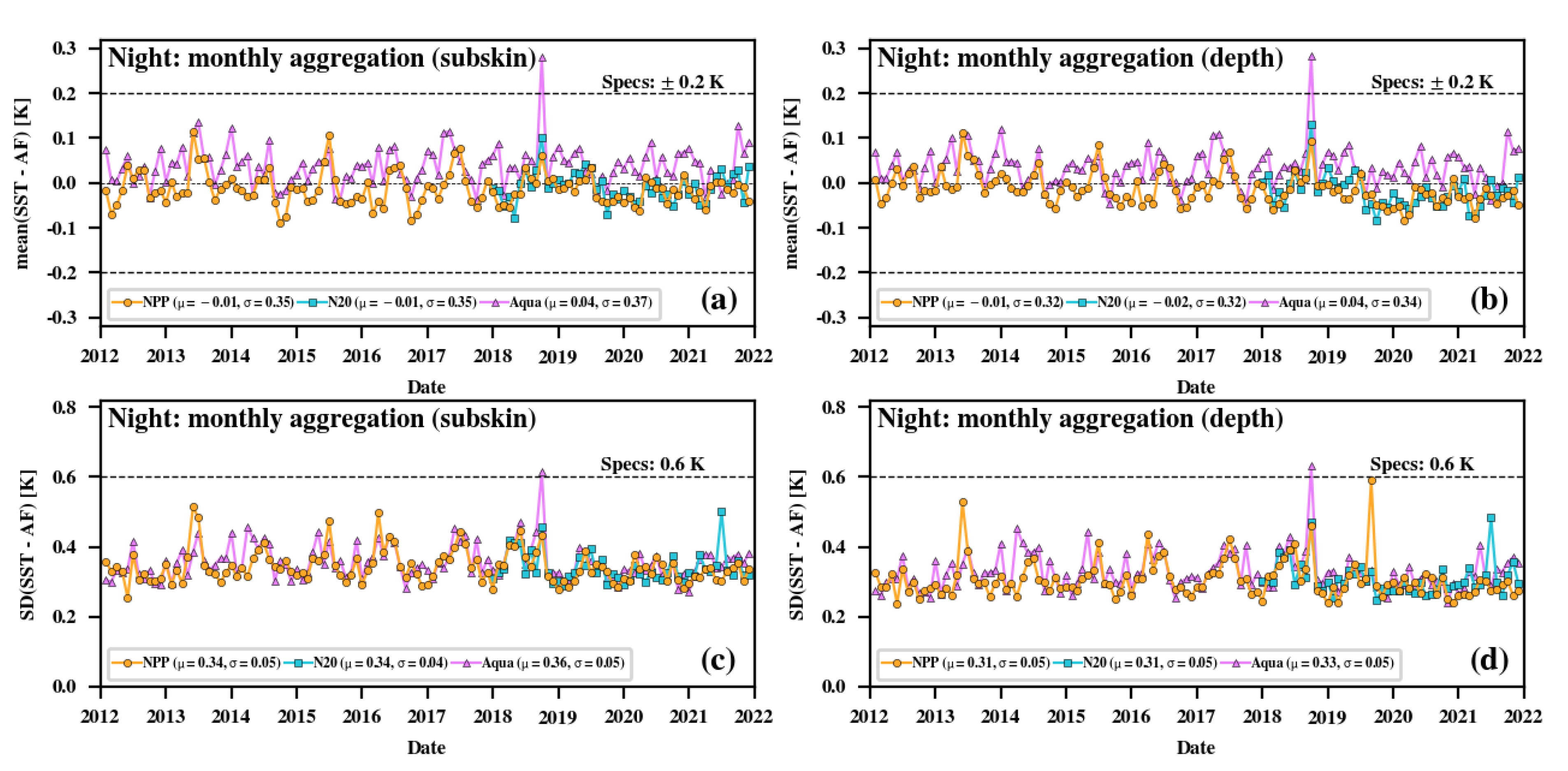
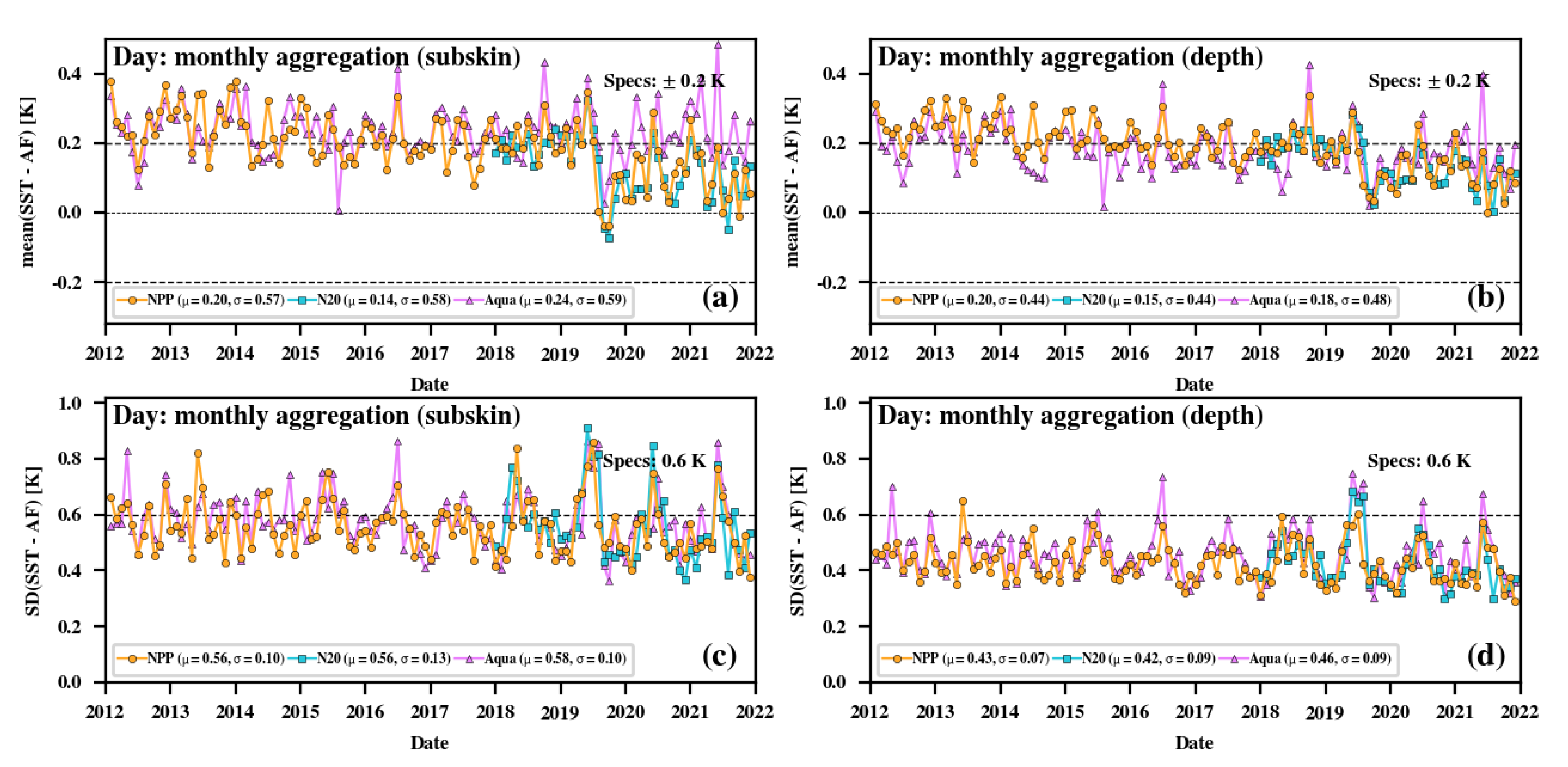
ACSPO VIIRS RAN3 SST was validated against quality-controlled in situ SST data from the NOAA iQuam system [24,25]. We found that NOAA SST requirements of ±0.2 K for accuracy (global mean bias wrt in situ SST) and 0.6 K for precision (global standard deviation) are generally met and often exceeded by a wide margin (especially at night), when compared against SSTs from (D+TM)’s, and independent Argo floats. Similar comparisons of Aqua MODIS ACSPO SSTs with in situ SSTs shows a 0.01–0.05 K improvement in VIIRS SST precision over MODIS, with larger margin during the daytime. We attribute those improvements to a combined effect of the inclusion of the M14 band centered at 8.6 µm in the ACSPO SST retrieval equations, and considerably higher VIIRS resolution (0.75 km vs. 1 km near nadir and 1.5 km vs. 5 km near the swath edge).

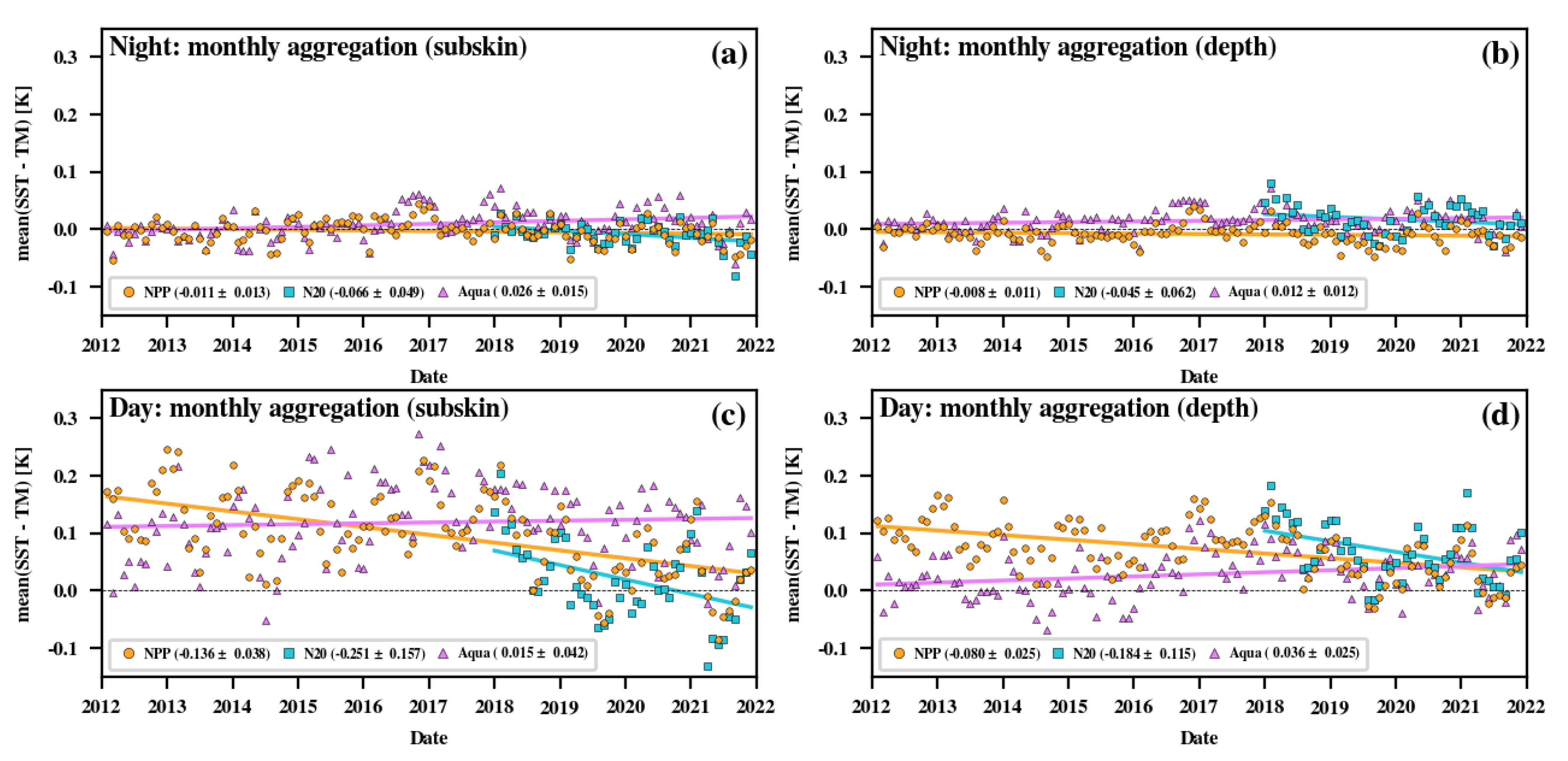
Stability of ACSPO VIIRS and MODIS SSTs was investigated by comparison of satellite SST against in situ SST from tropical moorings. Nighttime VIIRS and MODIS SSTs show excellent temporal stability. The NPP VIIRS SSTs show statistically insignificant trends of (−0.011 ± 0.013) K/decade for ‘subskin’ and (−0.008 ± 0.011) K/decade for ‘depth’ SST. For the preliminary MODIS-Aqua ACSPO SSTs, the trends are (+0.026 ± 0.015) K/decade for ‘subskin’ and (+0.012 ± 0.012) K/decade for ‘depth’ SST. For daytime SSTs, there is evidence of persistent negative VIIRS SST trends (for NPP, (−0.136 ± 0.038) K/decade for ‘subskin’ and (−0.080 ± 0.025) K/decade for ‘depth’ SSTs). Corresponding Aqua MODIS SST trends are much smaller, (+0.015 ± 0.042) K/decade for ‘subskin’ and (+0.036 ± 0.025) K/decade for ‘depth’ SSTs. Stability estimates using tropical moorings are expected to provide a more stringent estimate of sensor stability, due to the increased atmospheric correction required for the tropical atmosphere with high concentrations of water vapor.

A second independent validation of stability was performed by comparing double difference (DD) of daytime and nighttime mean biases against in situ SSTs from (D+TM)s, and CMC L4 analysis. DDs reduce the impact of instability in reference SST data (from either buoys or L4 analyses), if those are present in reference data. The excellent stability of VIIRS and MODIS nighttime SSTs suggests that day–night DDs are a good proxy for stability of daytime SST. The day–night DD analyses were largely consistent with validation against tropical moorings, but with lower uncertainties due to the several orders of magnitude larger in situ and L4 data volumes. For NPP VIIRS, DD-based estimates of the daytime SST trends were (−0.143 ± 0.015) K/decade for ‘subskin’ and (−0.078 ± 0.007) K/decade for ‘depth’ SSTs, largely consistent with the TM-based estimates. For Aqua MODIS, no statistically significant drift was found, with (+0.013 ± 0.014) K/decade for ‘subskin’ and (0.006 ± 0.011) K/decade for ‘depth’ SSTs. N20 SST stability was largely consistent with the NPP results but with higher uncertainties, due to the shorter duration of the N20 mission.

We also investigated stability of VIIRS brightness temperatures by comparing observed (O) BTs with those modeled (M), using the community radiative transfer model (CRTM) in the NOAA MICROS system [26,27,38]. To mitigate systematic biases in modeled BTs introduced by the CRTM inputs (SST and atmospheric profiles), we calculated double differences of the corresponding O-M biases between sensors (N20—NPP and Aqua—NPP). The agreement between NPP and Aqua bands centered at 3.7 µm is excellent, with a statistically insignificant relative trend of (−0.003 ± 0.004) K/decade at night. Agreement between the NPP and Aqua 12 µm bands was also good, with a relative trend of (−0.013 ± 0.003) at night and (+0.012 ± 0.004) K/decade during the daytime. The VIIRS 3.7 and 12 µm bands are the two main contributors to the nighttime SST; therefore, the excellent stability and inter-sensor consistency of VIIRS and MODIS nighttime SSTs was not surprising, given the stability of BTs in these two bands. For the band centered at 11 µm, there was a clear negative trend in NPP VIIRS BTs compared to Aqua MODIS, of (−0.024 ± 0.003) K/decade at night and (−0.041 ± 0.003) K/decade during the daytime. The negative trend had the same sign but a larger magnitude, compared to the value of −0.02 K/decade estimated by the authors in Reference [50] based on their comparison of VIIRS and CrIS near-nadir daytime and nighttime BTs from March 2012–February 2017. The 11 µm band is the main contributor to ACSPO daytime SST, and a negative drift in this VIIRS band is consistent with our observations of the negative trend in VIIRS daytime SST. We did not see statistically significant evidence of MODIS-Aqua daytime SST trend and, thus, concluded that the 11 µm band likely drifts on both VIIRSs. On Aqua MODIS, the 11 µm band is more stable. We did not find evidence of any drift between the NPP and N20 VIIRS thermal bands, suggesting that their 11 µm bands are drifting in-sync, at a similar rate on both satellites. We estimate that the observed (−0.041 ± 0.003) K/decade drift of the VIIRS thermal bands would cause a ~−0.09 K/decade drift in VIIRS daytime SST, which cannot fully explain the observed daytime ‘subskin’ SST drift of (−0.143 ± 0.015) K/decade. It is possible that the 8.6 µm band also contributes to VIIRS SST daytime trends. However, due to the suboptimal performance of the Aqua band 29 centered at 8.6 µm, estimating the stability of the VIIRS 8.6 µm band is challenging. We are not aware of any work, which estimates its stability with uncertainty sufficiently low to assist in the SST stability analysis (note that CrIS does not have spectral coverage near 3.7 µm and 8.6 µm and was not included in the analysis in Reference [50]).

Future ACSPO VIIRS work will include investigation of VIIRS thermal bands stability and its application to mitigation of daytime SST bias drift. We plan to perform a more detailed analysis of the stability of VIIRS thermal bands, including comparison with MODIS flown onboard Terra. We will also consider comparison with ABI/AHI sensors flown onboard GOES-R/Himawari series satellites in geostationary orbit, with Himawari-8 SST data going back to 2015 and GOES-16 to 2017. ABI and AHI sensors may provide further insight since in addition to having thermal bands centered near 11 and 12 µm, they also have bands centered near 8.6 µm. The new VIIRS sensors (with the next addition to the JPSS series, JPSS-2, planned for launch in September 2022) will be included in the analyses.

Future work will be also directed at better understanding of the validation results, in particular the 0.05 K ‘warm step’ in validation against (D+TM)’s after 2016, and approximately 0.10 K ‘cold step’ in validation against Argo floats and increased noise after mid- 2019. Analyses and reconciliation of in situ data are underway and will be reported elsewhere.

References

1. Petrenko, B.; Ignatov, A.; Kihai, Y.; Heidinger, A. Clear-Sky Mask for the Advanced Clear-Sky Processor for Ocean. J. Atmos. Ocean. Technol. 2010, 27, 1609. [Google Scholar] [CrossRef]
2. Petrenko, B.; Ignatov, A.; Kihai, Y.; Stroup, J.; Dash, P. Evaluation and Selection of SST Regression Algorithms for JPSS VIIRS: Selection of SST Regression Algorithms. J. Geophys. Res. Atmos. 2014, 119, 4580. [Google Scholar] [CrossRef]
3. Petrenko, B.; Ignatov, A.; Kihai, Y.; Dash, P. Sensor-Specific Error Statistics for SST in the Advanced Clear-Sky Processor for Oceans. J. Atmos. Ocean. Technol. 2016, 33, 345. [Google Scholar] [CrossRef]
4. Ignatov, A.; Gladkova, I.; Ding, Y.; Shahriar, F.; Kihai, Y.; Zhou, X. JPSS VIIRS Level 3 Uncollated Sea Surface Temperature Product at NOAA. J. Appl. Remote Sens. 2017, 11, 032405. [Google Scholar] [CrossRef]
5. Pryamitsyn, V.; Petrenko, B.; Ignatov, A.; Kihai, Y. Metop First Generation AVHRR FRAC SST Reanalysis Version 1. Remote Sens. 2021, 13, 4046. [Google Scholar] [CrossRef]
6. Pryamitsyn, V.; Ignatov, A.; Petrenko, B.; Jonasson, O.; Kihai, Y. Evaluation of the Initial NOAA AVHRR GAC SST Reanalysis Version 2 (RAN2 B01). Proc. SPIE 2022, 11420, 1142005. Available online: https://spie.org/Publications/Proceedings/Paper/10.1117/12.2558751?SSO=1 (accessed on 13 July 2022).
7. NOAA/STAR. GHRSST NPP VIIRS ACSPO V2.80 0.75 km L2P SST Dataset (GDS v2); PO.DAAC: Pasadena, CA, USA. Available online: https://doi.org/10.5067/GHVRS-2PO28 (accessed on 13 July 2022).
8. NOAA/STAR. GHRSST NPP VIIRS ACSPO V2.80 0.02° L3U SST Dataset (GDS v2); PO.DAAC: Pasadena, CA, USA. Available online: https://doi.org/10.5067/GHVRS-3UO28 (accessed on 13 July 2022).
9. NOAA/STAR. GHRSST N20 VIIRS ACSPO V2.80 0.75 km L2P SST Dataset (GDS v2); PO.DAAC: Pasadena, CA, USA. Available online: https://doi.org/10.5067/GHV20-2PO28 (accessed on 13 July 2022).
10. NOAA/STAR. GHRSST N20 VIIRS ACSPO V2.80 0.02° L3U SST Dataset (GDS v2); PO.DAAC: Pasadena, CA, USA. Available online: https://doi.org/10.5067/GHV20-3UO28 (accessed on 13 July 2022).
11. Cao, C.; Xiong, X.; Wolfe, R.; DeLuccia, F.; Liu, Q.; Blonski, S.; Lin, G.; Nishihama, M.; Pogorzala, D.; Oudrari, H.; et al. Visible Infrared Imaging Radiometer Suite (VIIRS) Sensor Data Record (SDR) User’s Guide Version 1. NOAA Tech. Rep. NESDIS 2013, 142. Available online: https://nsidc.org/sites/nsidc.org/files/technical-references/VIIRS-SDR-users-guide.pdf (accessed on 13 July 2022).
12. The Group for High Resolution Sea Surface Temperature Science Team; Casey, K.; Donlon, C. The Recommended Ghrsst Data Specification (GDS). Available online: https://zenodo.org/record/4700466#.Yr0ZVuxBxPZ (accessed on 13 July 2022).
13. Jonasson, O.; Gladkova, I.; Ignatov, A.; Kihai, Y. Progress with Development of Global Gridded Super-Collated SST Products from Low Earth Orbiting Satellites (L3S-LEO) at NOAA. Proc. SPIE 2020, 11420, 1142002. [Google Scholar] [CrossRef]
14. Jonasson, O.; Gladkova, I.; Ignatov, A.; Kihai, Y. Algorithmic Improvements and Consistency Checks of the NOAA Global Gridded Super-Collated SSTs from Low Earth Orbiting Satellites (L3S-LEO). Proc. SPIE 2021, 11752, 1175202. [Google Scholar] [CrossRef]
15. NOAA/STAR. GHRSST L3S-LEO-PM ACSPO V2.80 0.02° L3S SST Dataset (GDS v2) from Afternoon LEO Satellites; PO.DAAC: Pasadena, CA, USA. Available online: https://doi.org/10.5067/GHLPM-3SS28 (accessed on 13 July 2022).
16. NOAA/STAR. ACSPO Global SST from VIIRS. NOAA CoastWatch & OceanWatch. Available online: https://coastwatch.noaa.gov/cw/satellite-data-products/sea-surface-temperature/acspo-viirs.html (accessed on 13 July 2022).
17. NOAA/STAR. GHRSST L3S-LEO ACSPO V2.80 0.02-degree L3S SST Dataset (GDS v2) from Low-Earth-Orbiting Platforms (L3S-LEO). Available online: https://coastwatch.noaa.gov/cw/satellite-data-products/sea-surface-temperature/noaa-acspo/l3s-leo.html (accessed on 13 July 2022).
18. Dash, P.; Ignatov, A.; Kihai, Y.; Sapper, J. The SST Quality Monitor (SQUAM). J. Atmospheric Ocean. Technol. 2010, 27, 1899. [Google Scholar] [CrossRef]
19. ACSPO Regional Monitor for SST v2.1 (ARMS). Available online: https://www.star.nesdis.noaa.gov/socd/sst/arms (accessed on 13 July 2022).
20. Jonasson, O.; Ignatov, A. Status of Second VIIRS Reanalysis (RAN2). Proc. SPIE 2019, 11014, 110140O. [Google Scholar] [CrossRef]
21. Wang, W.; Cao, C.; Ignatov, A.; Liang, X.; Li, Z.; Wang, L.; Zhang, B.; Blonski, S.; Li, J. Improving the Calibration of Suomi NPP VIIRS Thermal Emissive Bands During Blackbody Warm-Up/Cool-Down. IEEE Trans. Geosci. Remote Sens. 2019, 57, 1977. [Google Scholar] [CrossRef]
22. STAR. Integrated Calibration/Validation System (ICVS)-Long-Term Monitoring. Available online: https://www.star.nesdis.noaa.gov/icvs (accessed on 13 July 2022).
23. Gladkova, I.; Ignatov, A.; Shahriar, F.; Kihai, Y.; Hillger, D.; Petrenko, B. Improved VIIRS and MODIS SST Imagery. Remote Sens. 2016, 8, 79. [Google Scholar] [CrossRef] [Green Version]
24. Xu, F.; Ignatov, A. In Situ SST Quality Monitor (iQuam). J. Atmospheric Ocean. Technol. 2014, 31, 164. [Google Scholar] [CrossRef]
25. In Situ SST Quality Monitor System (iQuam). Available online: https://www.star.nesdis.noaa.gov/socd/sst/iquam (accessed on 13 July 2022).
26. Liu, Q.; van Delst, P.; Chen, Y.; Groff, D.; Han, Y.; Collard, A.; Weng, F.; Boukabara, S.; Derber, J. Community Radiative Transfer Model for Radiance Assimilation and Applications. IEEE Int. Geosci. Remote Sens. Symp. 2012, 3700–3703. [Google Scholar] [CrossRef]
27. Liang, X.-M.; Ignatov, A.; Kihai, Y. Implementation of the Community Radiative Transfer Model in Advanced Clear-Sky Processor for Oceans and Validation against Nighttime AVHRR Radiances. J. Geophys. Res. Atmos. 2009, 114, D06112. [Google Scholar] [CrossRef]
28. Walton, C.C.; Pichel, W.G.; Sapper, J.F.; May, D.A. The Development and Operational Application of Nonlinear Algorithms for the Measurement of Sea Surface Temperatures with the NOAA Polar-Orbiting Environmental Satellites. J. Geophys. Res.Ocean. 1998, 103, 27999. [Google Scholar] [CrossRef]
29. Barton, I.J. Digitization Effects in AVHRR and MCSST Data. Remote Sens. Environ. 1989, 29, 87–89. [Google Scholar] [CrossRef]
30. Merchant, C.J.; Le Borgne, P.; Roquet, H.; Legendre, G. Extended Optimal Estimation Techniques for Sea Surface Temperature from the Spinning Enhanced Visible and Infra-Red Imager. Remote. Sens. Environ. 2013, 131, 287–297. [Google Scholar] [CrossRef]
31. Petrenko, B.; Ignatov, A.; Kihai, Y. Suppressing the noise in SST retrieved from satellite infrared measurements by smoothing the differential terms in regression equations. Proc. SPIE 2015, 9459. [Google Scholar] [CrossRef]
32. Sun, J.; Wang, M. Electronic Crosstalk in Aqua MODIS Long-Wave Infrared Photovoltaic Bands. Remote Sens. 2016, 8, 806. [Google Scholar] [CrossRef] [Green Version]
33. Minnett, P.J.; Kilpatrick, K.A.; Podestá, G.P.; Evans, R.H.; Szczodrak, M.D.; Izaguirre, M.A.; Williams, E.J.; Walsh, S.; Reynolds, R.M.; Bailey, S.W.; et al. Skin Sea-Surface Temperature from VIIRS on Suomi-NPP—NASA Continuity Retrievals. Remote Sens. 2020, 12, 3369. [Google Scholar] [CrossRef]
34. JPL/OBPG/RSMAS. GHRSST Level 2P Global Sea Surface Skin Temperature from the Visible and Infrared Imager/Radiometer Suite (VIIRS) on the Suomi-NPP Satellite (GDS2). Available online: https://doi.org/10.5067/GHVRS-2PJ62 (accessed on 13 July 2022).
35. Cayula, J.-F.P.; May, D.A.; McKenzie, B.D.; Willis, K.D. VIIRS-Derived SST at the Naval Oceanographic Office: From Evaluation to Operation. SPIE Proc. 2013, 8724, 274–281. [Google Scholar] [CrossRef]
36. Naval Oceanographic Office (NAVO). GHRSST Level 2P 1m Depth Global Sea Surface Temperature Version 3.0 from the Visible Infrared Imaging Radiometer Suite (VIIRS) on the Suomi NPP Satellite (GDS2); PO.DAAC: Pasadena, CA, USA. Available online: https://doi.org/10.5067/GHVRS-2PN30 (accessed on 13 July 2022).
37. Canada Meteorological Center. GHRSST Level 4 CMC0.1deg Global Foundation Sea Surface Temperature Analysis (GDS v2); PO.DAAC: Pasadena, CA, USA. Available online: https://doi.org/10.5067/GHCMC-4FM03 (accessed on 13 July 2022).
38. Liang, X.; Ignatov, A. Monitoring of IR Clear-Sky Radiances over Oceans for SST (MICROS). J. Atmos. Ocean. Technol. 2011, 28, 1228. [Google Scholar] [CrossRef] [Green Version]
39. Gladkova, I.; Kihai, Y.; Ignatov, A.; Shahriar, F.; Petrenko, B. SST Pattern Test in ACSPO clear-sky mask for VIIRS. Remote Sens. Environ. 2015, 160, 87–98. [Google Scholar] [CrossRef]
40. Gould, J.; Roemmich, D.; Wijffels, S.; Freeland, H.; Ignaszewsky, M.; Jianping, X.; Pouliquen, S.; Desaubies, Y.; Send, U.; Radhakrishnan, K.; et al. Argo Profiling Floats Bring New Era of in Situ Ocean Observations. EOS Trans. Am. Geophys. Union 2004, 85, 185. [Google Scholar] [CrossRef]
41. Roemmich, D.; The Argo Steering Team. Argo: The challenge of continuing 10 years of progress. Oceanography 2009, 22, 46. [Google Scholar] [CrossRef]
42. Wong, A.; Keeley, R.; Carval, T.; the Argo Data Management Team. Argo Quality Control Manual for CTD and Trajectory Data. 2022. Available online: https://doi.org/10.13155/33951 (accessed on 13 July 2022).
43. Xu, F.; Ignatov, A. Error Characterization in iQuam SSTs Using Triple Collocations with Satellite Measurements. Geophys. Res. Lett. 2016, 43, 10826. [Google Scholar] [CrossRef]
44. Merchant, C.J.; Embury, O.; Rayner, N.A.; Berry, D.I.; Corlett, G.K.; Lean, K.; Veal, K.L.; Kent, E.C.; Llewellyn-Jones, D.T.; Remedios, J.J.; et al. A 20 Year Independent Record of Sea Surface Temperature for Climate from Along-Track Scanning Radiometers. J. Geophys. Res. Oceans 2012, 117, C12013. [Google Scholar] [CrossRef] [Green Version]
45. Cleveland, R.B.; Cleveland, W.S.; McRae, J.E.; Terpenning, I. STL: A Seasonal-Trend Decomposition Procedure Based on Loess. J. Off. Stat. 1990, 6, 3. [Google Scholar]
46. Seabold, S.; Perktold, J. Statsmodels: Econometric and Statistical Modeling with Python. In Proceedings of the 9th Python in Science Conference, Austin, TX, USA, 28 June–3 July 2010; pp. 92–96. [Google Scholar] [CrossRef] [Green Version]
47. CMC. GHRSST Level 4 CMC0.2deg Global Foundation Sea Surface Temperature Analysis (GDS v2); PO.DAAC: Pasadena, CA, USA. Available online: https://doi.org/10.5067/GHCMC-4FM02 (accessed on 13 July 2022).
48. Rienecker, M.M.; Suarez, M.J.; Gelaro, R.; Todling, R.; Bacmeister, J.; Liu, E.; Bosilovich, M.G.; Schubert, S.D.; Takacs, L.; Kim, G.-K.; et al. MERRA: NASA’s Modern-Era Retrospective Analysis for Research and Applications. J. Clim. 2011, 24, 3624. [Google Scholar] [CrossRef]
49. NCEP. Global Forecast System (GFS). Available online: https://www.emc.ncep.noaa.gov/emc/pages/numerical_forecast_systems/gfs/documentation.php (accessed on 13 July 2022).
50. Cao, C.; Zhang, B.; Shao, X.; Wang, W.; Uprety, S.; Choi, T.; Blonski, S.; Gu, Y.; Bai, Y.; Lin, L.; et al. Mission-Long Recalibrated Science Quality Suomi NPP VIIRS Radiometric Dataset Using Advanced Algorithms for Time Series Studies. Remote Sens. 2021, 13, 1075. [Google Scholar] [CrossRef]
51. Gladkova, I.; Ignatov, A.; Pennybacker, M.; Kihai, Y. Towards High-Resolution Multi-Sensor Gridded ACSPO SST Product: Reducing Residual Cloud Contamination. Proc. SPIE 2019, 11014, 110140L. [Google Scholar] [CrossRef]
52. NOAA/STAR. GHRSST L3S-LEO-AM ACSPO V2.80 0.02° L3S Dataset from Mid-Morning LEO Satellites (GDS v2); PO.DAAC: Pasadena, CA, USA. Available online: https://doi.org/10.5067/GHLAM-3SS28 (accessed on 13 July 2022).
53. NAVO. GHRSST Level 2P Global 1 Meter Sea Surface Temperature from the Visible Infrared Imaging Radiometer Suite (VIIRS) on the Suomi NPP Satellite (GDS v2). Version 1.0. Available online: https://doi.org/10.5067/GHVRS-2PN02 (accessed on 13 July 2022).
54. NAVO. GHRSST Level 2P Global 1 Meter Sea Surface Temperature from the Visible Infrared Imaging Radiometer Suite (VIIRS) on the Suomi NPP Satellite (GDS v2). Version 2.0. Available online: https://doi.org/10.5067/GHVRS-2PN01 (accessed on 13 July 2022).
Figure 1. Monthly mean sensitivity (on a 0.1° × 0.1° latitude/longitude grid) for ACSPO V2.80 NPP VIIRS daytime ‘subskin’ SST for May 2020. In most cases, it is close to 1 (except in the tropical regions, and especially at slant VZAs, where atmospheric humidity is high, and the sensitivity can be as low as 0.8).
Remotesensing 14 03476 g001
Figure 2. ACSPO NPP ‘subskin’-(D+TM) SST for the full year of 2020, stratified by (a) latitude and (b) retrieved ‘subskin’ SST in RAN2 (produced with ACSPO V2.61) and RAN3 (produced with ACSPO V2.80). The number of observations (NOBS) in the RAN3 datasets is denoted by gray histograms. Bins with NOBS < 5% of the median NOBS were omitted.
Remotesensing 14 03476 g002
Figure 3. ACSPO N20 VIIRS nighttime L2P SST imagery over the Chesapeake Bay on 13 September 2021. (a) ACSPO V2.80 all-sky ‘subskin’ SST (no mask applied); (b) ΔSST = ‘subskin’−CMC L4 SST (pixels with ΔSST < −2 K are shown in black); (c) same as (a) but with the V2.80 mask applied (gray pixels); (d) same as (c) except the mask is now from V2.61. Note that over-screening of cold ΔSSTs is significantly reduced in V2.80.
Remotesensing 14 03476 g003
Figure 4. ACSPO NPP VIIRS nighttime L2P SST over the Chesapeake Bay on 14 November 2020: (a) all-sky imagery (no ACSM overlaid); (b) the same scene but with the ACSM V2.80 applied (gray overlay) and thermal fronts overlaid (in black). Land is rendered in brown. Images are from the NOAA ACSPO Regional Monitor for SST online system (ARMS) [19].
Remotesensing 14 03476 g004
Figure 5. Aggregated for year 2020 maps of nighttime N20 VIIRS ‘subskin’-(D+TM) SST. The figure is from the NOAA SST Quality Monitor (SQUAM) online system [18].
Remotesensing 14 03476 g005
Figure 6. Aggregated for year 2020 histograms of ACSPO-(D+TM) SST for N20: (a,b) night; (c,d) day; (a,c) ‘subskin’ SST (computed using global regression, GR); (b,d) ‘depth’ SST (computed using piecewise regression, PWR). Figures are from the NOAA SQUAM system [18].
Remotesensing 14 03476 g006
Figure 7. Times series of 24 h aggregated nighttime ACSPO-(D+TM) SSTs: (a,b) accuracy (global mean bias); (c,d) precision (corresponding SD); (a,c) ‘subskin’ SST (computed using global regression, GR); (b,d) ‘depth’ SST (computed using piecewise regression, PWR). Temporal means and SDs of the 24 h aggregated accuracy and precision are given by µ and σ, respectively. Data are from the NOAA SQUAM system [18].
Remotesensing 14 03476 g007
Figure 8. Panels (ad) show the same results as in Figure 7 but for the daytime.
Remotesensing 14 03476 g008
Figure 9. Aggregated for year 2020 maps of nighttime N20 VIIRS ‘subskin’-AF SST. The figure is from the NOAA SST Quality Monitor (SQUAM) online system [18].
Remotesensing 14 03476 g009
Figure 10. Panels (ad) show the same results as Figure 6 but against the AFs.
Remotesensing 14 03476 g010
Figure 11. Panels (ad) show the same results as Figure 7 but for monthly aggregated statistics against AFs.
Remotesensing 14 03476 g011
Figure 12. Panels (ad) show the same results as in Figure 11 but for daytime.
Remotesensing 14 03476 g012
Figure 13. Time series of monthly aggregated nighttime ACSPO−TM SST mean biases: (a,b) nighttime; (c,d) daytime; (a,c) ‘subskin’ SST (computed using global regression, GR); (b,d) ‘depth’ SST (computed using piecewise regression, PWR). For each time series, the slope (obtained using a linear least square fit) in units of K/decade is overlaid, along with the associated uncertainty obtained using a 95% confidence interval. Lines show the corresponding linear fits.
Remotesensing 14 03476 g013
Figure 14. Time series of monthly aggregated ‘day minus night’ DDs calculated from (a,b) ACSPO−(D+TM); (c,d) ACSPO−L4 ΔSSTs for (a,c) ‘subskin’; (b,d) ‘depth’ SSTs. Slopes (K/decade; obtained using a linear least squares fit) are provided, along with the associated uncertainties obtained using a 95% confidence interval. Lines show the corresponding linear fits.
Remotesensing 14 03476 g014
Figure 15. Panels (ah) show monthly aggregated DDs of mean O−M BTs biases in thermal bands centered at: (a,b) 3.7 µm; (c,d) 8.6 µm; (e,f) 11 µm; (g,h) 12 µm; (i,j) corresponding DDs for satellite ‘subskin’ minus CMC L4 SST [37,47]). Left (a,c,e,g,i) and right (b,d,f,h,j) panels show nighttime and daytime results, respectively. Slopes (K/decade; from a linear least squares fit) are shown, along with their uncertainty obtained using a 95% confidence interval. Symbols represent monthly aggregated mean DDs and lines show the corresponding linear fits. Note that the CMC L4 SST is a model input into CRTM results presented in (ah). Data are from the NOAA MICROS online system [38].
Remotesensing 14 03476 g015