
An Investigation of the Ice Cloud Detection Sensitivity of Cloud Radars Using the Raman Lidar at the ARM SGP Site


Abstract
:
1. Introduction
2. Data and Model
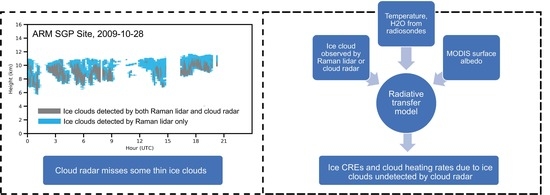
2.1. Raman Lidar and Cloud Radars
2.2. Radiative Transfer Model
3. Results
3.1. Cloud Occurrence Fraction
3.2. Ice COD
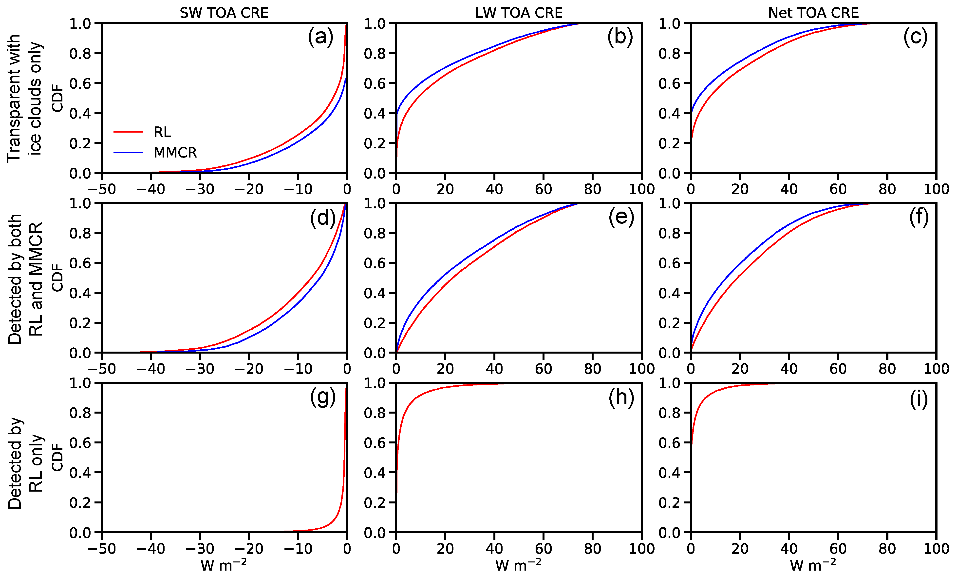
3.3. Ice CREs
4. Discussion and Conclusions
Supplementary Materials
Author Contributions
Funding
Data Availability Statement
Acknowledgments
Conflicts of Interest
References
- Berry, E.; Mace, G.G. Cloud properties and radiative effects of the Asian summer monsoon derived from A—Train data. J. Geophys. Res. Atmos. 2014, 119, 9492–9508. [Google Scholar] [CrossRef]
- Dupont, J.-C.; Haeffelin, M. Observed instantaneous cirrus radiative effect on surface-level shortwave and longwave irradiances. J. Geophys. Res. Atmos. 2008, 113, D21202. [Google Scholar] [CrossRef]
- Liou, K.-N. Influence of Cirrus Clouds on Weather and Climate Processes: A Global Perspective. Mon. Weather Rev. 1986, 114, 1167–1199. [Google Scholar] [CrossRef]
- Lolli, S.; Campbell, J.R.; Lewis, J.R.; Gu, Y.; Marquis, J.W.; Chew, B.N.; Liew, S.-C.; Salinas, S.V.; Welton, E.J. Daytime Top-of-the-Atmosphere Cirrus Cloud Radiative Forcing Properties at Singapore. J. Appl. Meteorol. Clim. 2017, 56, 1249–1257. [Google Scholar] [CrossRef] [Green Version]
- Sherwood, S.C. On moistening of the tropical troposphere by cirrus clouds. J. Geophys. Res. Atmos. 1999, 104, 11949–11960. [Google Scholar] [CrossRef]
- Fu, Q.; Hu, Y.; Yang, Q. Identifying the top of the tropical tropopause layer from vertical mass flux analysis and CALIPSO lidar cloud observations. Geophys. Res. Lett. 2007, 34. [Google Scholar] [CrossRef] [Green Version]
- Lin, L.; Fu, Q.; Zhang, H.; Su, J.; Yang, Q.; Sun, Z. Upward mass fluxes in tropical upper troposphere and lower stratosphere derived from radiative transfer calculations. J. Quant. Spectrosc. Radiat. Transf. 2013, 117, 114–122. [Google Scholar] [CrossRef]
- Sun, W.; Baize, R.R.; Videen, G.; Hu, Y.; Fu, Q. A method to retrieve super-thin cloud optical depth over ocean background with polarized sunlight. Atmos. Chem. Phys. 2015, 15, 11909–11918. [Google Scholar] [CrossRef] [Green Version]
- Fu, Q.; Liou, K.N. Parameterization of the Radiative Properties of Cirrus Clouds. J. Atmos. Sci. 1993, 50, 2008–2025. [Google Scholar] [CrossRef] [Green Version]
- Heymsfield, A.J.; Krämer, M.; Luebke, A.; Brown, P.; Cziczo, D.J.; Franklin, C.; Lawson, P.; Lohmann, U.; McFarquhar, G.; Ulanowski, Z.; et al. Cirrus Clouds. Meteorol. Monogr. 2017, 58, 2.1–2.26. [Google Scholar] [CrossRef] [Green Version]
- Platt, C.M.R.; Harshvardhan. Temperature dependence of cirrus extinction: Implications for climate feedback. J. Geophys. Res. Atmos. 1988, 93, 11051–11058. [Google Scholar] [CrossRef]
- Zhang, Y.; Macke, A.; Albers, F. Effect of crystal size spectrum and crystal shape on stratiform cirrus radiative forcing. Atmos. Res. 1999, 52, 59–75. [Google Scholar] [CrossRef]
- Fu, Q.; Baker, M.; Hartmann, D.L. Tropical cirrus and water vapor: An effective Earth infrared iris feedback? Atmos. Chem. Phys. 2002, 2, 31–37. [Google Scholar] [CrossRef] [Green Version]
- Stephens, G.L.; Tsay, S.-C.; Stackhouse, P.W.; Flatau, P.J. The Relevance of the Microphysical and Radiative Properties of Cirrus Clouds to Climate and Climatic Feedback. J. Atmos. Sci. 1990, 47, 1742–1754. [Google Scholar] [CrossRef]
- Waliser, D.E.; Li, J.-L.F.; Woods, C.P.; Austin, R.T.; Bacmeister, J.; Chern, J.; Del Genio, A.; Jiang, J.H.; Kuang, Z.; Meng, H.; et al. Cloud ice: A climate model challenge with signs and expectations of progress. J. Geophys. Res. Atmos. 2009, 114, D00A21. [Google Scholar] [CrossRef]
- Balmes, K.A.; Fu, Q. An Investigation of Optically Very Thin Ice Clouds from Ground-Based ARM Raman Lidars. Atmosphere 2018, 9, 445. [Google Scholar] [CrossRef] [Green Version]
- Balmes, K.A.; Fu, Q.; Thorsen, T.J. Differences in Ice Cloud Optical Depth From CALIPSO and Ground-Based Raman Lidar at the ARM SGP and TWP Sites. J. Geophys. Res. Atmos. 2019, 124, 1755–1778. [Google Scholar] [CrossRef]
- Campbell, J.R.; Hlavka, D.L.; Welton, E.J.; Flynn, C.J.; Turner, D.D.; Spinhirne, J.D.; Scott, V.S.; Hwang, I.H. Full-Time, Eye-Safe Cloud and Aerosol Lidar Observation at Atmospheric Radiation Measurement Program Sites: Instruments and Data Processing. J. Atmos. Ocean. Technol. 2002, 19, 431–442. [Google Scholar] [CrossRef]
- Comstock, J.M.; Ackerman, T.P.; Turner, D.D. Evidence of high ice supersaturation in cirrus clouds using ARM Raman lidar measurements. Geophys. Res. Lett. 2004, 31, L11106. [Google Scholar] [CrossRef] [Green Version]
- Hollars, S.; Fu, Q.; Comstock, J.; Ackerman, T. Comparison of cloud-top height retrievals from ground-based 35 GHz MMCR and GMS-5 satellite observations at ARM TWP Manus site. Atmos. Res. 2004, 72, 169–186. [Google Scholar] [CrossRef]
- Sassen, K.; Campbell, J.R. A Midlatitude Cirrus Cloud Climatology from the Facility for Atmospheric Remote Sensing. Part I: Macrophysical and Synoptic Properties. J. Atmos. Sci. 2001, 58, 481–496. [Google Scholar] [CrossRef]
- Shupe, M.D.; Comstock, J.M.; Turner, D.D.; Mace, G.G. Cloud Property Retrievals in the ARM Program. Meteorol. Monogr. 2016, 57, 19.11–19.20. [Google Scholar] [CrossRef]
- Thorsen, T.J.; Fu, Q.; Comstock, J. Comparison of the CALIPSO satellite and ground-based observations of cirrus clouds at the ARM TWP sites. J. Geophys. Res. Atmos. 2011, 116, D21203. [Google Scholar] [CrossRef] [Green Version]
- Thorsen, T.J.; Fu, Q.; Comstock, J.M.; Sivaraman, C.; Vaughan, M.A.; Winker, D.M.; Turner, D.D. Macrophysical properties of tropical cirrus clouds from the CALIPSO satellite and from ground-based micropulse and Raman lidars. J. Geophys. Res. Atmos. 2013, 118, 9209–9220. [Google Scholar] [CrossRef]
- Goldsmith, J.E.M.; Blair, F.H.; Bisson, S.E.; Turner, D.D. Turn-key Raman lidar for profiling atmospheric water vapor, clouds, and aerosols. Appl. Opt. 1998, 37, 4979–4990. [Google Scholar] [CrossRef]
- Ferrare, R.; Turner, D.; Clayton, M.; Schmid, B.; Redemann, J.; Covert, D.; Elleman, R.; Ogren, J.; Andrews, E.; Goldsmith, J.E.M.; et al. Evaluation of daytime measurements of aerosols and water vapor made by an operational Raman lidar over the Southern Great Plains. J. Geophys. Res. Atmos. 2006, 111, D05S08. [Google Scholar] [CrossRef] [Green Version]
- Newsom, R. Raman lidar (RL) handbook. In Office of Scientific & Technical Information Technical Reports; Citeseer: University Park, PA, USA, 2009. [Google Scholar]
- Moran, K.P.; Martner, B.E.; Post, M.J.; Kropfli, R.A.; Welsh, D.C.; Widener, K.B. An Unattended Cloud-Profiling Radar for Use in Climate Research. Bull. Am. Meteorol. Soc. 1998, 79, 443–456. [Google Scholar] [CrossRef] [Green Version]
- Clothiaux, E.E.; Miller, M.A.; Perez, R.C.; Turner, D.D.; Moran, K.P.; Martner, B.E.; Ackerman, T.P.; Mace, G.G.; Marchand, R.T.; Widener, K.B. The ARM Millimeter Wave Cloud Radars (MMCRs) and the Active Remote Sensing of Clouds (ARSCL) Value Added Product (VAP); DOE Office of Science Atmospheric Radiation Measurement (ARM) User Facility; U.S. Department of Energy Office of Scientific and Technical Information: Oak Ridge, TN, USA, 2001.
- Fu, Q.; Carlin, B.; Mace, G. Cirrus horizontal inhomogeneity and OLR bias. Geophys. Res. Lett. 2000, 27, 3341–3344. [Google Scholar] [CrossRef] [Green Version]
- Carlin, B.; Fu, Q.; Lohmann, U.; Mace, G.G.; Sassen, K.; Comstock, J.M. High-Cloud Horizontal Inhomogeneity and Solar Albedo Bias. J. Clim. 2002, 15, 2321–2339. [Google Scholar] [CrossRef] [Green Version]
- Widener, K.; Bharadwaj, N.; Johnson, K. Ka-Band ARM Zenith Radar (KAZR) Instrument Handbook; DOE Office of Science Atmospheric Radiation Measurement (ARM) Program; U.S. Department of Energy Office of Scientific and Technical Information: Oak Ridge, TN, USA, 2012.
- Tinel, C.; Testud, J.; Pelon, J.; Hogan, R.J.; Protat, A.; Delanoë, J.; Bouniol, D. The Retrieval of Ice-Cloud Properties from Cloud Radar and Lidar Synergy. J. Appl. Meteorol. 2005, 44, 860–875. [Google Scholar] [CrossRef] [Green Version]
- Borg, L.A.; Holz, R.E.; Turner, D.D. Investigating cloud radar sensitivity to optically thin cirrus using collocated Raman lidar observations. Geophys. Res. Lett. 2011, 38, L05807. [Google Scholar] [CrossRef]
- Thorsen, T.J.; Fu, Q.; Newsom, R.K.; Turner, D.D.; Comstock, J.M. Automated Retrieval of Cloud and Aerosol Properties from the ARM Raman Lidar. Part I: Feature Detection. J. Atmos. Ocean. Technol. 2015, 32, 1977–1998. [Google Scholar] [CrossRef]
- Thorsen, T.J.; Fu, Q. Automated Retrieval of Cloud and Aerosol Properties from the ARM Raman Lidar. Part II: Extinction. J. Atmos. Ocean. Technol. 2015, 32, 1999–2023. [Google Scholar] [CrossRef]
- Fu, Q. An Accurate Parameterization of the Solar Radiative Properties of Cirrus Clouds for Climate Models. J. Clim. 1996, 9, 2058–2082. [Google Scholar] [CrossRef] [Green Version]
- Fu, Q.; Liou, K.N. On the Correlated k-Distribution Method for Radiative Transfer in Nonhomogeneous Atmospheres. J. Atmos. Sci. 1992, 49, 2139–2156. [Google Scholar] [CrossRef] [Green Version]
- Fu, Q.; Yang, P.; Sun, W.B. An Accurate Parameterization of the Infrared Radiative Properties of Cirrus Clouds for Climate Models. J. Clim. 1998, 11, 2223–2237. [Google Scholar] [CrossRef]
- Rose, F.; Charlock, T. New Fu-Liou code tested with ARM raman lidar aerosols and CERES in pre-CALIPSO sensitivity study. In Proceedings of the 11th Conference on Atmospheric Radiation, Ogden, UT, USA, 3–7 June 2002. [Google Scholar]
- Rose, F.; Charlock, T.; Fu, Q.; Kato, S.; Rutan, D.; Jin, Z. CERES proto-edition 3 radiative transfer: Model tests and radiative closure over surface validation sites. In Proceedings of the 12th Conference on Atmospheric Radiation, Madison, WI, USA, 9–14 July 2006. [Google Scholar]
- Wu, X.; Balmes, K.A.; Fu, Q. Aerosol Direct Radiative Effects at the ARM SGP and TWP Sites: Clear Skies. J. Geophys. Res. Atmos. 2021, 126, e2020JD033663. [Google Scholar] [CrossRef]
- Balmes, K.A.; Fu, Q. All-Sky Aerosol Direct Radiative Effects at the ARM SGP Site. J. Geophys. Res. Atmos. 2021, 126, e2021JD034933. [Google Scholar] [CrossRef]
- Morris, V. Microwave Radiometer (MWR) Handbook; DOE Office of Science Atmospheric Radiation Measurement (ARM) Program; U.S. Department of Energy Office of Scientific and Technical Information: Oak Ridge, TN, USA, 2019.
- Turner, D.D.; Vogelmann, A.M.; Austin, R.T.; Barnard, J.C.; Cady-Pereira, K.; Chiu, J.C.; Clough, S.A.; Flynn, C.; Khaiyer, M.M.; Liljegren, J.; et al. Thin Liquid Water Clouds: Their Importance and Our Challenge. Bull. Am. Meteorol. Soc. 2007, 88, 177–190. [Google Scholar] [CrossRef]
- Dee, D.P.; Uppala, S.M.; Simmons, A.J.; Berrisford, P.; Poli, P.; Kobayashi, S.; Andrae, U.; Balmaseda, M.A.; Balsamo, G.; Bauer, P.; et al. The ERA-Interim reanalysis: Configuration and performance of the data assimilation system. Q. J. R. Meteorol. Soc. 2011, 137, 553–597. [Google Scholar] [CrossRef]
- Yang, Q.; Fu, Q.; Austin, J.; Gettelman, A.; Li, F.; Vömel, H. Observationally derived and general circulation model simulated tropical stratospheric upward mass fluxes. J. Geophys. Res. Atmos. 2008, 113, D00B07. [Google Scholar] [CrossRef] [Green Version]
- Roesch, A.; Schaaf, C.; Gao, F. Use of Moderate-Resolution Imaging Spectroradiometer bidirectional reflectance distribution function products to enhance simulated surface albedos. J. Geophys. Res. Atmos. 2004, 109, D12105. [Google Scholar] [CrossRef] [Green Version]
- Schaaf, C.B.; Gao, F.; Strahler, A.H.; Lucht, W.; Li, X.; Tsang, T.; Strugnell, N.C.; Zhang, X.; Jin, Y.; Muller, J.-P.; et al. First operational BRDF, albedo nadir reflectance products from MODIS. Remote Sens. Environ. 2002, 83, 135–148. [Google Scholar] [CrossRef] [Green Version]
- Heymsfield, A.; Winker, D.; Avery, M.; Vaughan, M.; Diskin, G.; Deng, M.; Mitev, V.; Matthey, R. Relationships between Ice Water Content and Volume Extinction Coefficient from In Situ Observations for Temperatures from 0° to −86 °C: Implications for Spaceborne Lidar Retrievals. J. Appl. Meteorol. Clim. 2014, 53, 479–505. [Google Scholar] [CrossRef]
- Hong, Y.; Liu, G.; Li, J.-L.F. Assessing the Radiative Effects of Global Ice Clouds Based on CloudSat and CALIPSO Measurements. J. Clim. 2016, 29, 7651–7674. [Google Scholar] [CrossRef]
- Ewald, F.; Groß, S.; Wirth, M.; Delanoë, J.; Fox, S.; Mayer, B. Why we need radar, lidar, and solar radiance observations to constrain ice cloud microphysics. Atmos. Meas. Tech. 2021, 14, 5029–5047. [Google Scholar] [CrossRef]


| COD | SW TOA CRE | LW TOA CRE | Net TOA CRE | SW SFC CRE | LW SFC CRE | Net SFC CRE | |||||||
|---|---|---|---|---|---|---|---|---|---|---|---|---|---|
| (W m−2) | (W m−2) | (W m−2) | (W m−2) | (W m−2) | (W m−2) | ||||||||
| Transparent with ice clouds only | |||||||||||||
| RL | 0.30 | −6.72 | (−1.35) | 22.27 | (4.47) | 15.54 | (3.12) | −7.04 | (−1.41) | 4.24 | (0.85) | −2.8 | (−0.56) |
| MMCR | 0.24 | −5.22 | (−1.05) | 17.45 | (3.5) | 12.23 | (2.45) | −5.6 | (−1.12) | 3.6 | (0.72) | −2 | (−0.4) |
| MMCR-RL | −0.06 | 1.51 | (0.3) | −4.82 | (−0.97) | −3.31 | (−0.66) | 1.43 | (0.29) | −0.63 | (−0.13) | 0.8 | (0.16) |
| (MMCR–RL)/RL | −20.3% | −22.4% | −21.6% | −21.3% | −20.4% | −15% | −28.6% | ||||||
| Transparent with ice clouds only and detected by both RL and MMCR (63.1%) | |||||||||||||
| RL | 0.46 | −10.00 | (−1.27) | 33.48 | (4.24) | 23.48 | (2.97) | −10.67 | (−1.35) | 6.51 | (0.82) | −4.17 | (−0.53) |
| MMCR | 0.38 | −8.26 | (−1.05) | 27.64 | (3.5) | 19.38 | (2.45) | −8.87 | (−1.12) | 5.71 | (0.72) | −3.17 | (−0.4) |
| MMCR-RL | −0.08 | 1.73 | (0.22) | −5.84 | (−0.74) | −4.11 | (−0.52) | 1.8 | (0.23) | −0.8 | (−0.1) | 1 | (0.13) |
| (MMCR–RL)/RL | −17.7% | −17.4% | −17.5% | −17.5% | −16.9% | −12.3% | −24% | ||||||
| Transparent with ice clouds only and detected by RL only (36.9%) | |||||||||||||
| RL | 0.03 | −1.12 | (−0.08) | 3.06 | (0.23) | 1.94 | (0.14) | −0.81 | (−0.06) | 0.35 | (0.03) | −0.46 | (−0.03) |
| MMCR | 0 | 0 | (0) | 0 | (0) | 0 | (0) | 0 | (0) | 0 | (0) | 0 | (0) |
| MMCR-RL | −0.03 | 1.12 | (0.08) | −3.06 | (−0.23) | −1.94 | (−0.14) | 0.81 | (0.06) | −0.35 | (−0.03) | 0.46 | (0.03) |
| (MMCR–RL)/RL | — | — | — | — | — | — | — | ||||||
| COD | SW TOA CRE | LW TOA CRE | Net TOA CRE | SW SFC CRE | LW SFC CRE | Net SFC CRE | |||||||
|---|---|---|---|---|---|---|---|---|---|---|---|---|---|
| (W m−2) | (W m−2) | (W m−2) | (W m−2) | (W m−2) | (W m−2) | ||||||||
| Transparent with ice clouds only | |||||||||||||
| RL | 0.31 | −6.92 | (−1.39) | 23.17 | (4.65) | 16.24 | (3.26) | −7.39 | (−1.48) | 4.48 | (0.9) | −2.93 | (−0.59) |
| KAZR | 0.26 | −5.66 | (−1.14) | 19.09 | (3.83) | 13.42 | (2.69) | −6.2 | (−1.24) | 3.99 | (0.8) | −2.22 | (−0.45) |
| KAZR-RL | −0.05 | 1.26 | (0.25) | −4.09 | (−0.82) | −2.82 | (−0.57) | 1.19 | (0.24) | −0.48 | (−0.1) | 0.71 | (0.14) |
| (KAZR–RL)/RL | −14.9% | −18.3% | −17.6% | −17.4% | −16.1% | −10.8% | −24.2% | ||||||
| Transparent with ice clouds only and detected by both RL and KAZR (63.0%) | |||||||||||||
| RL | 0.47 | −10.15 | (−1.28) | 34.28 | (4.33) | 24.12 | (3.05) | −11.07 | (−1.4) | 6.85 | (0.87) | −4.23 | (−0.53) |
| KAZR | 0.42 | −8.98 | (−1.14) | 30.22 | (3.82) | 21.24 | (2.69) | −9.84 | (−1.24) | 6.32 | (0.8) | −3.51 | (−0.44) |
| KAZR-RL | −0.05 | 1.18 | (0.15) | −4.06 | (−0.51) | −2.88 | (−0.36) | 1.24 | (0.16) | −0.52 | (−0.07) | 0.71 | (0.09) |
| (KAZR–RL)/RL | −11.2% | −11.6% | −11.8% | −11.9% | −11.2% | −7.6% | −16.9% | ||||||
| Transparent with ice clouds only and detected by RL only (37.0%) | |||||||||||||
| RL | 0.04 | −1.41 | (−0.1) | 4.13 | (0.31) | 2.71 | (0.2) | −1.12 | (−0.08) | 0.42 | (0.03) | −0.7 | (−0.05) |
| KAZR | 0 | 0 | (0) | 0 | (0) | 0 | (0) | 0 | (0) | 0 | (0) | 0 | (0) |
| KAZR-RL | −0.04 | 1.41 | (0.1) | −4.13 | (−0.31) | −2.71 | (−0.2) | 1.12 | (0.08) | −0.42 | (−0.03) | 0.7 | (0.05) |
| (KAZR–RL)/RL | — | — | — | — | — | — | — | ||||||
Publisher’s Note: MDPI stays neutral with regard to jurisdictional claims in published maps and institutional affiliations. |
© 2022 by the authors. Licensee MDPI, Basel, Switzerland. This article is an open access article distributed under the terms and conditions of the Creative Commons Attribution (CC BY) license (https://creativecommons.org/licenses/by/4.0/).
Share and Cite
Wang, M.; Balmes, K.A.; Thorsen, T.J.; Willick, D.; Fu, Q. An Investigation of the Ice Cloud Detection Sensitivity of Cloud Radars Using the Raman Lidar at the ARM SGP Site. Remote Sens. 2022, 14, 3466. https://doi.org/10.3390/rs14143466
Wang M, Balmes KA, Thorsen TJ, Willick D, Fu Q. An Investigation of the Ice Cloud Detection Sensitivity of Cloud Radars Using the Raman Lidar at the ARM SGP Site. Remote Sensing. 2022; 14(14):3466. https://doi.org/10.3390/rs14143466
Chicago/Turabian StyleWang, Mingcheng, Kelly A. Balmes, Tyler J. Thorsen, Dylan Willick, and Qiang Fu. 2022. "An Investigation of the Ice Cloud Detection Sensitivity of Cloud Radars Using the Raman Lidar at the ARM SGP Site" Remote Sensing 14, no. 14: 3466. https://doi.org/10.3390/rs14143466