
Towards an Integrated Observational System to Investigate Sediment Transport in the Tidal Inlets of the Lagoon of Venice

 , , ,
, , , 
Abstract
:1. Introduction
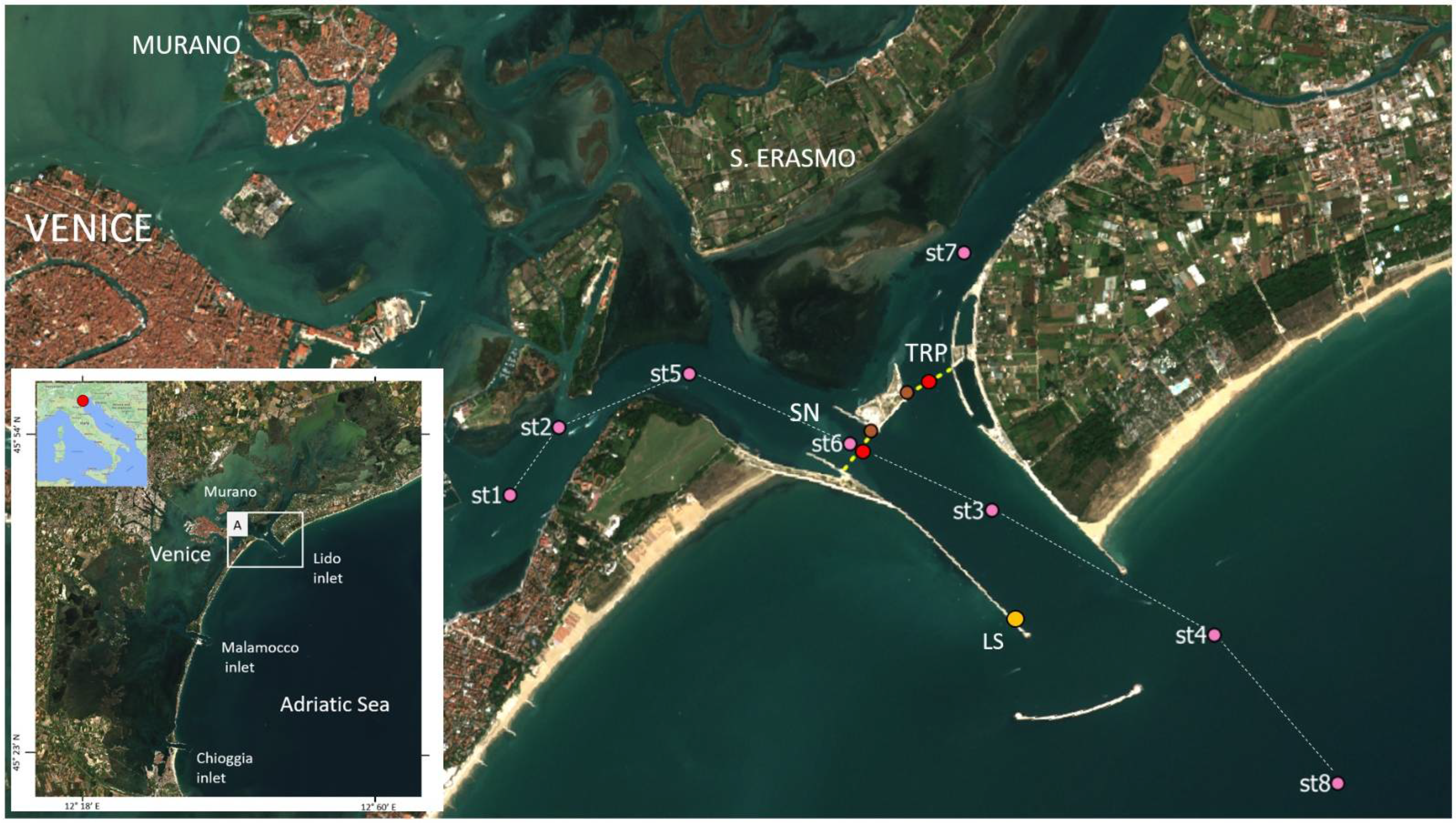
2. Study Area
3. Materials and Methods
3.1. In Situ Monitoring Network
3.2. In-Field Activities
3.3. Remote Sensing Data
4. Results and Discussion
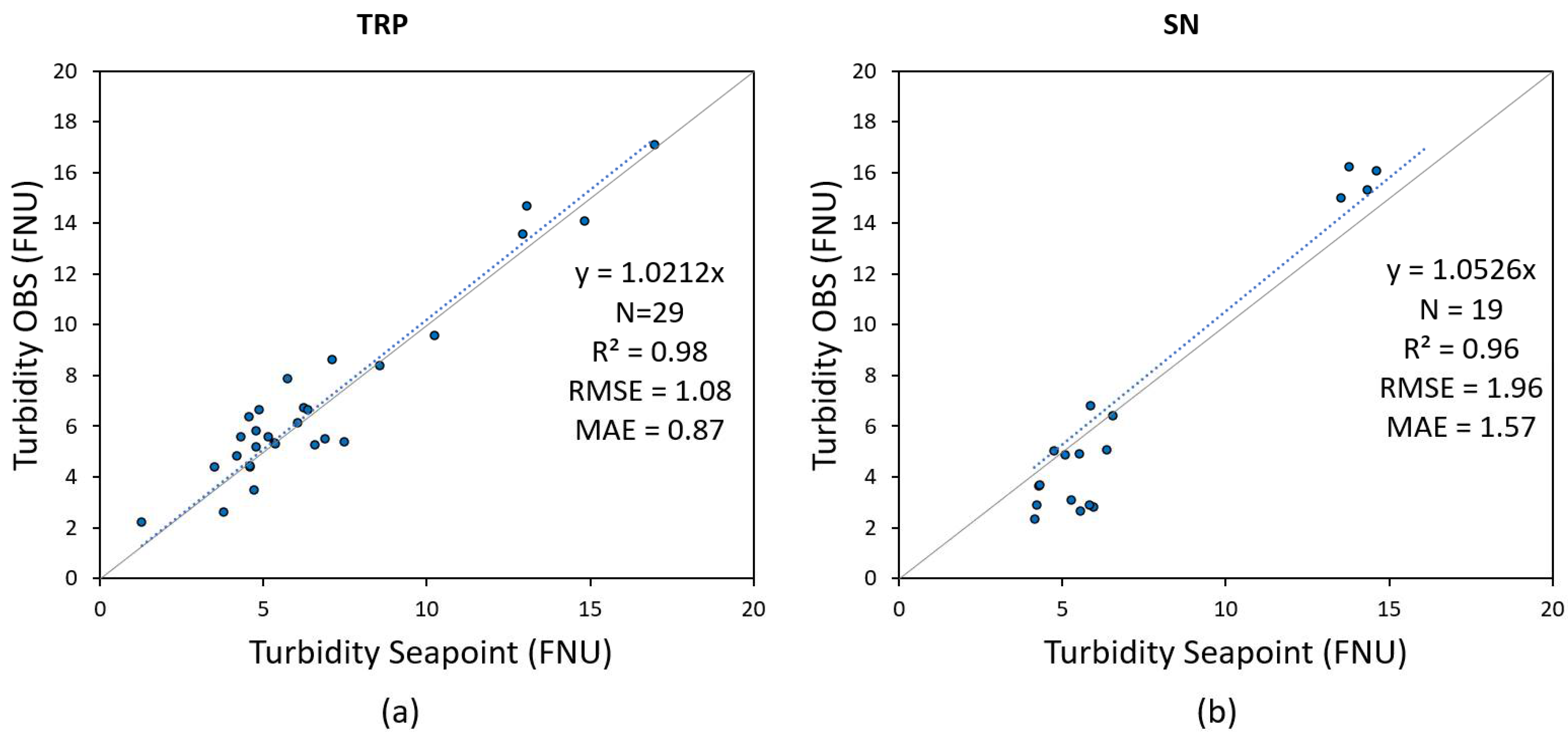
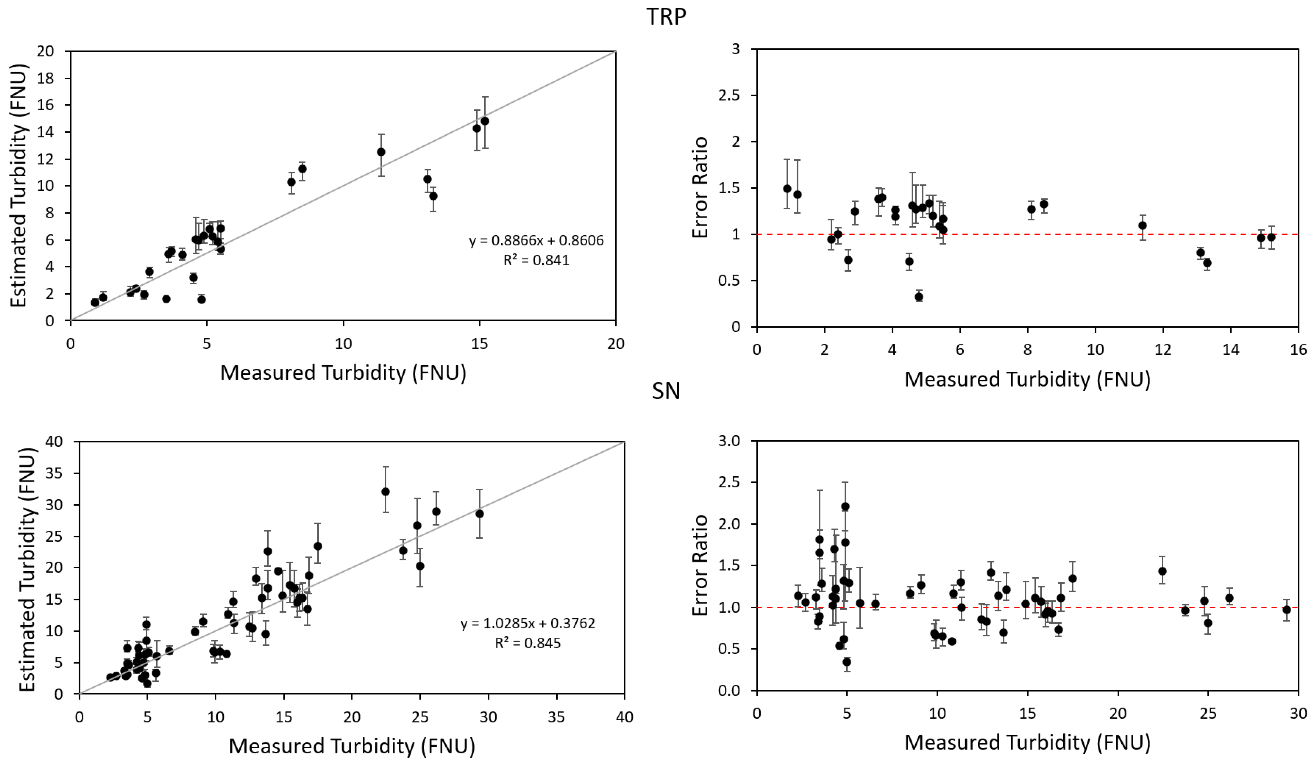
4.1. Intercalibration of Turbidimeters
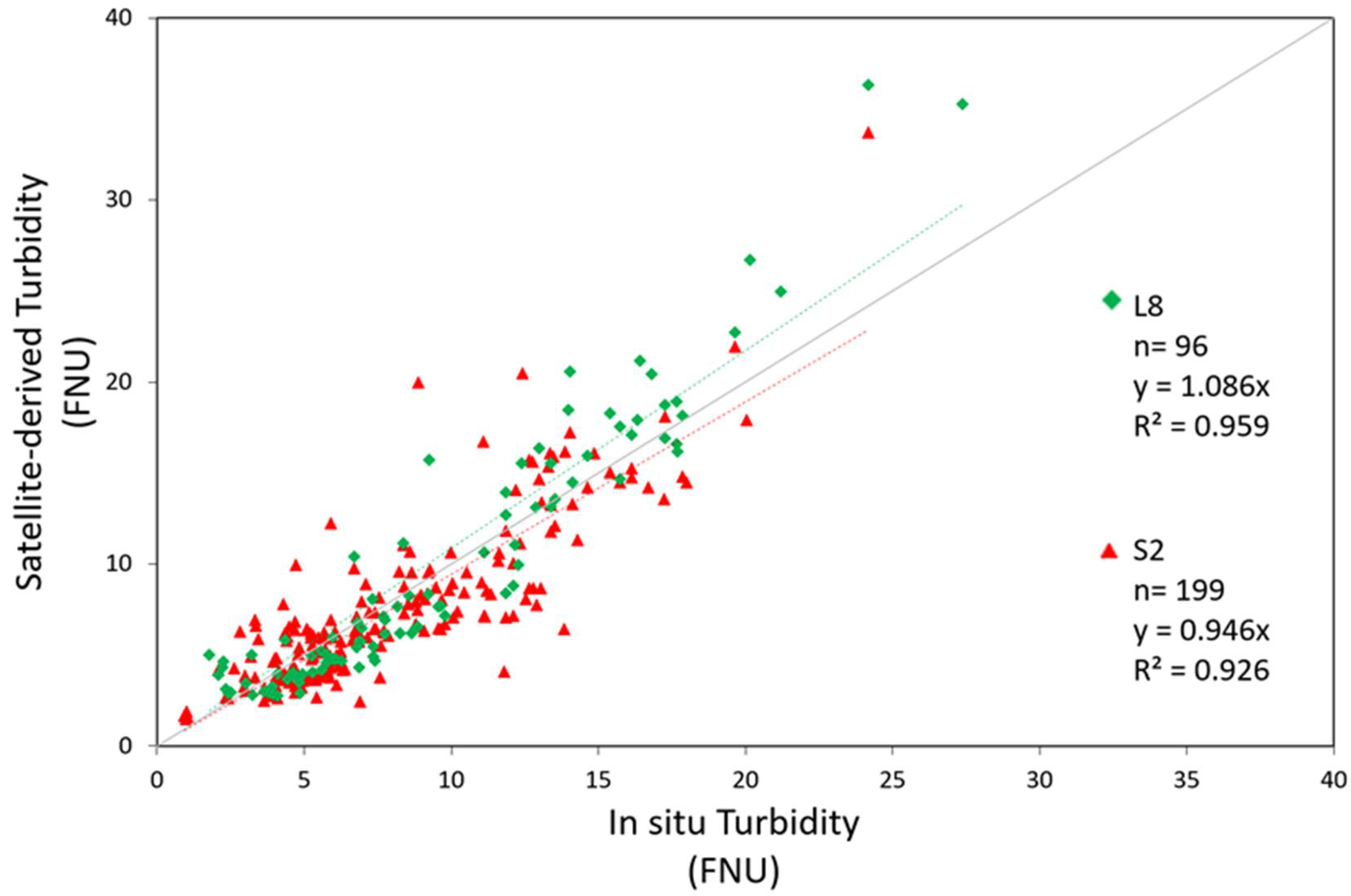
4.2. Validation of Satellite-Derived Products
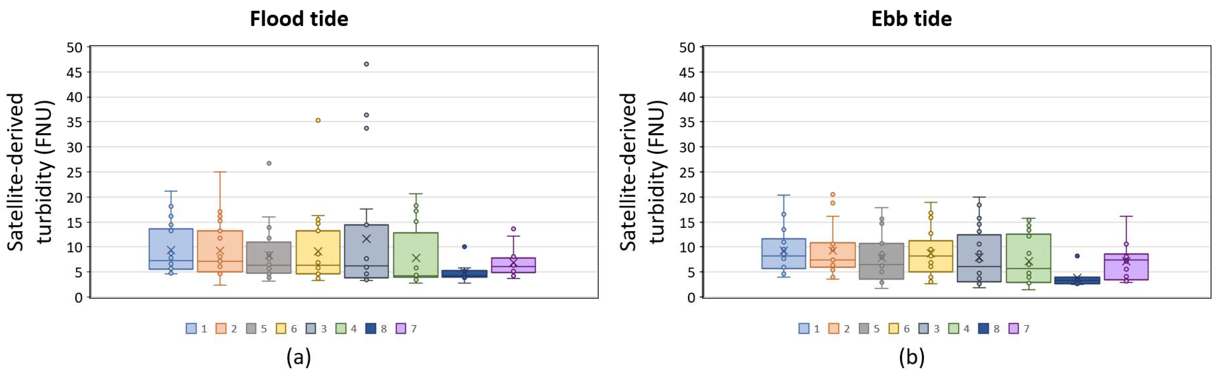
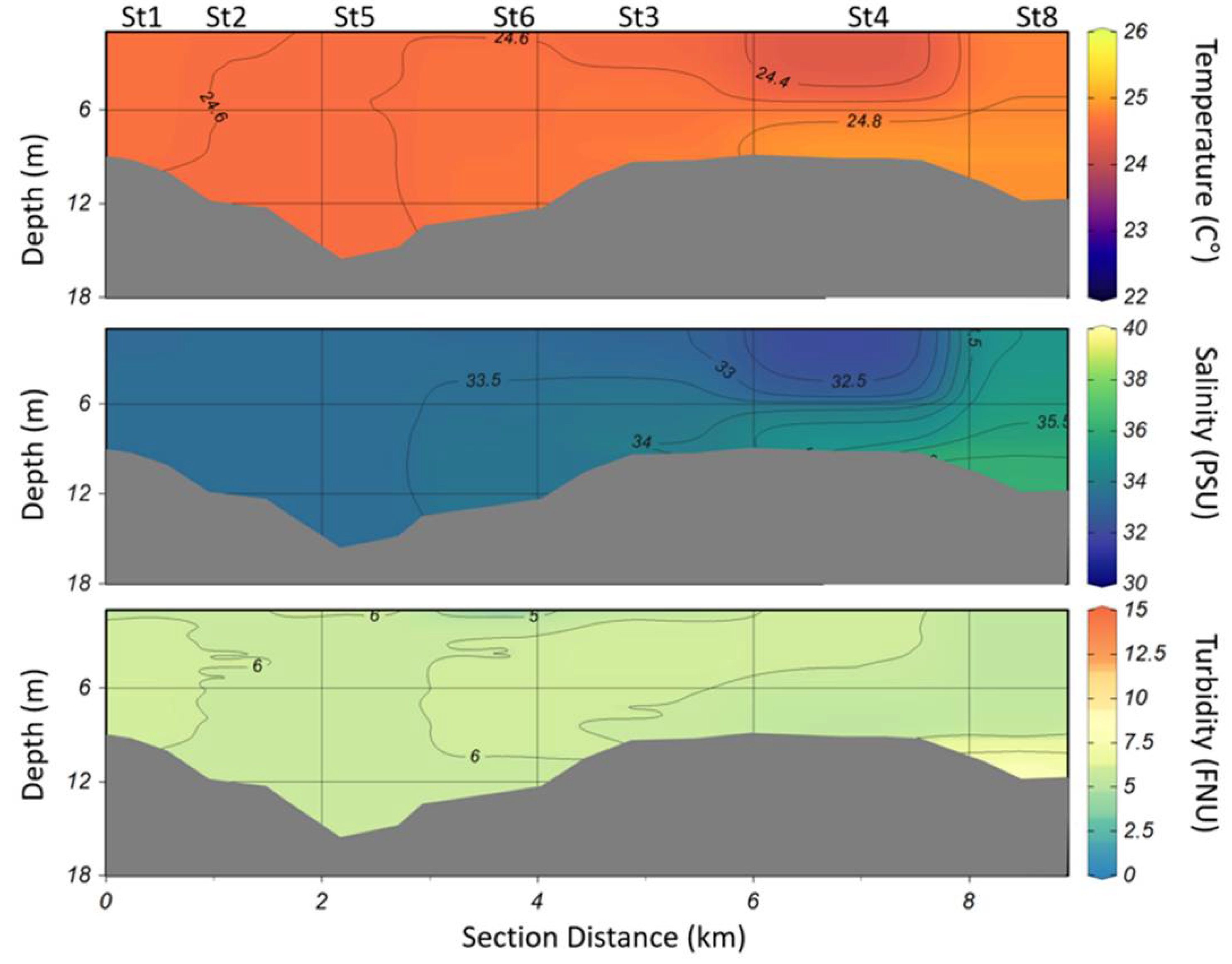
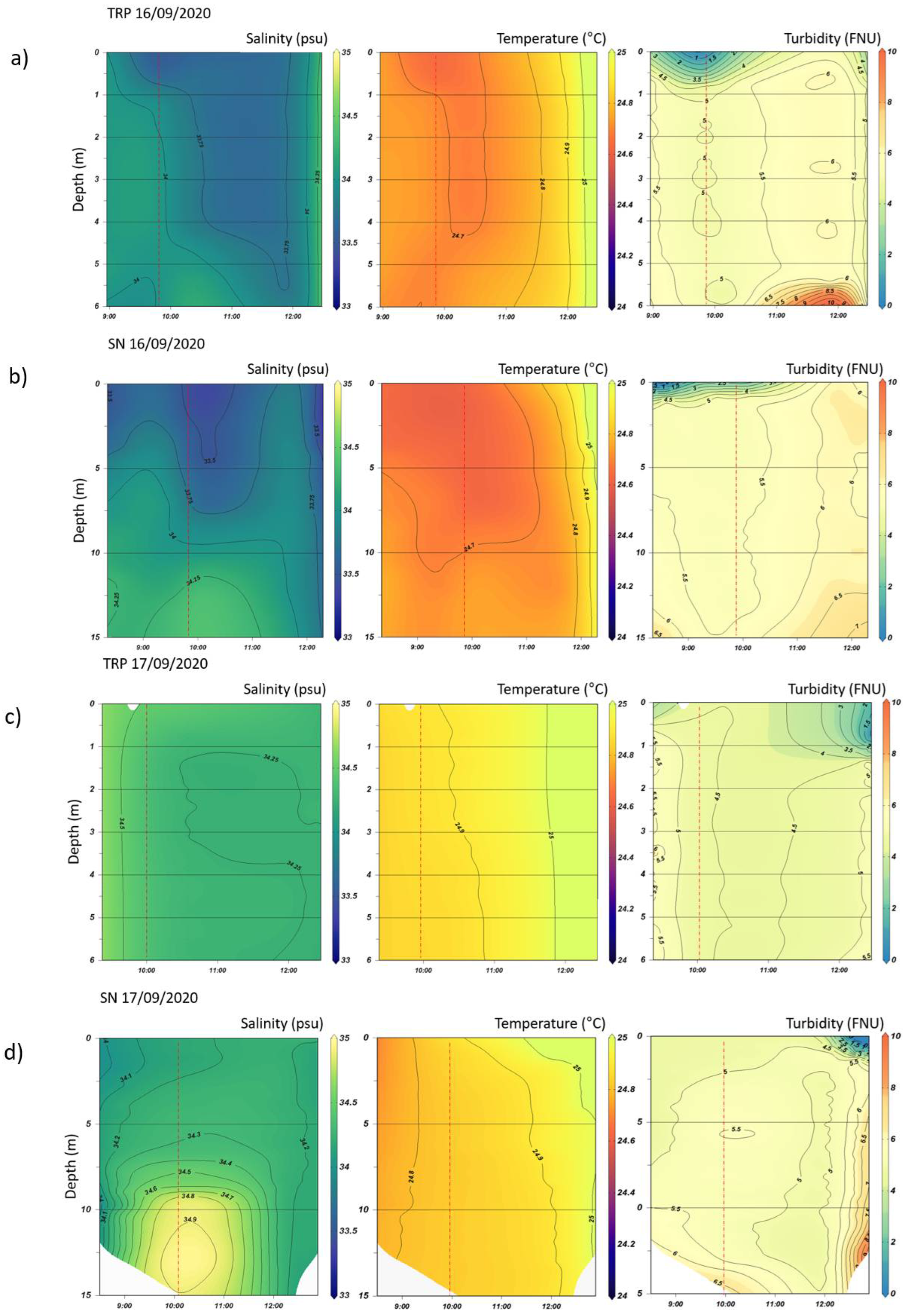
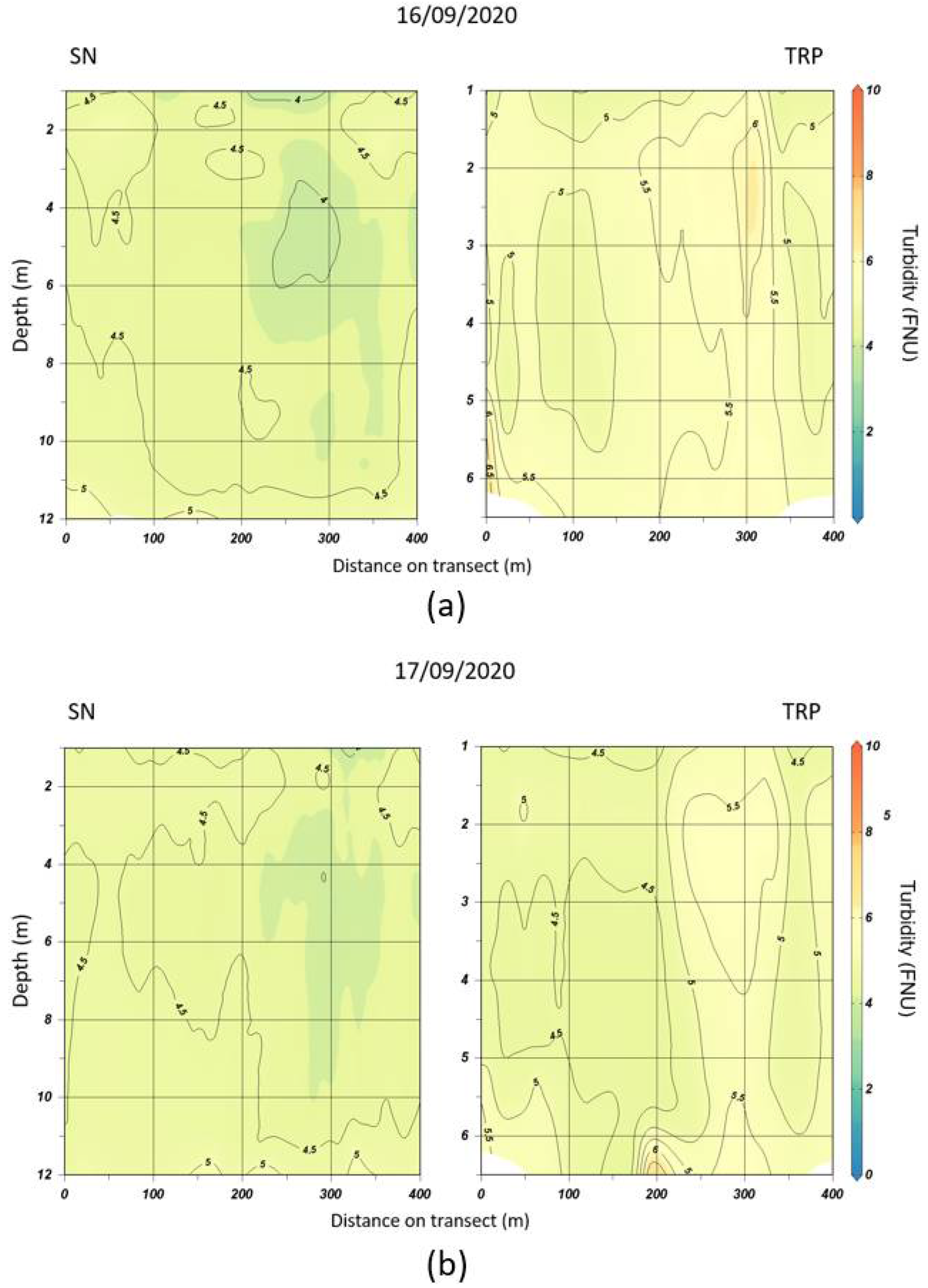
4.3. Spatial Turbidity Distribution in the Lagoon–Sea Transect
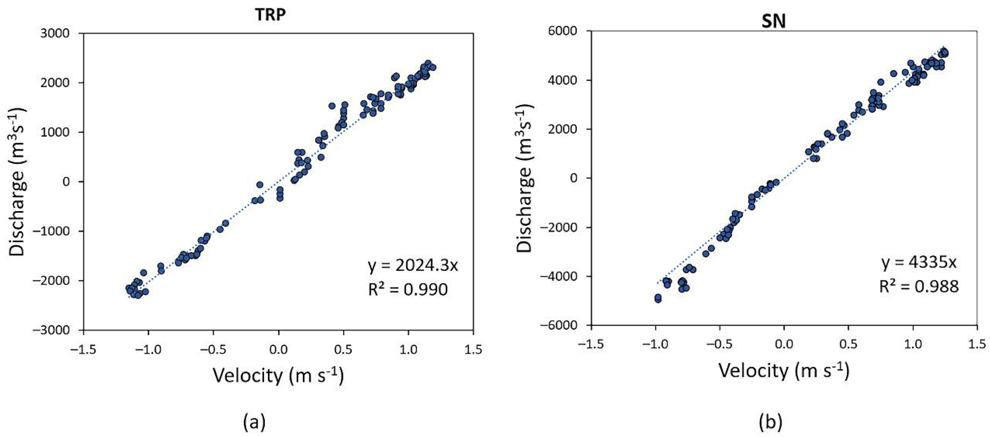
4.4. Discharge Calibration
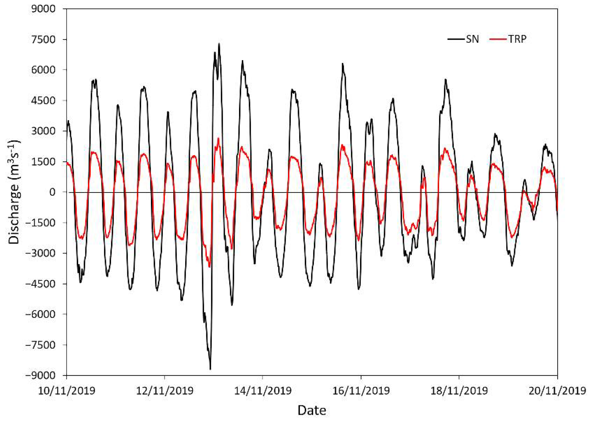
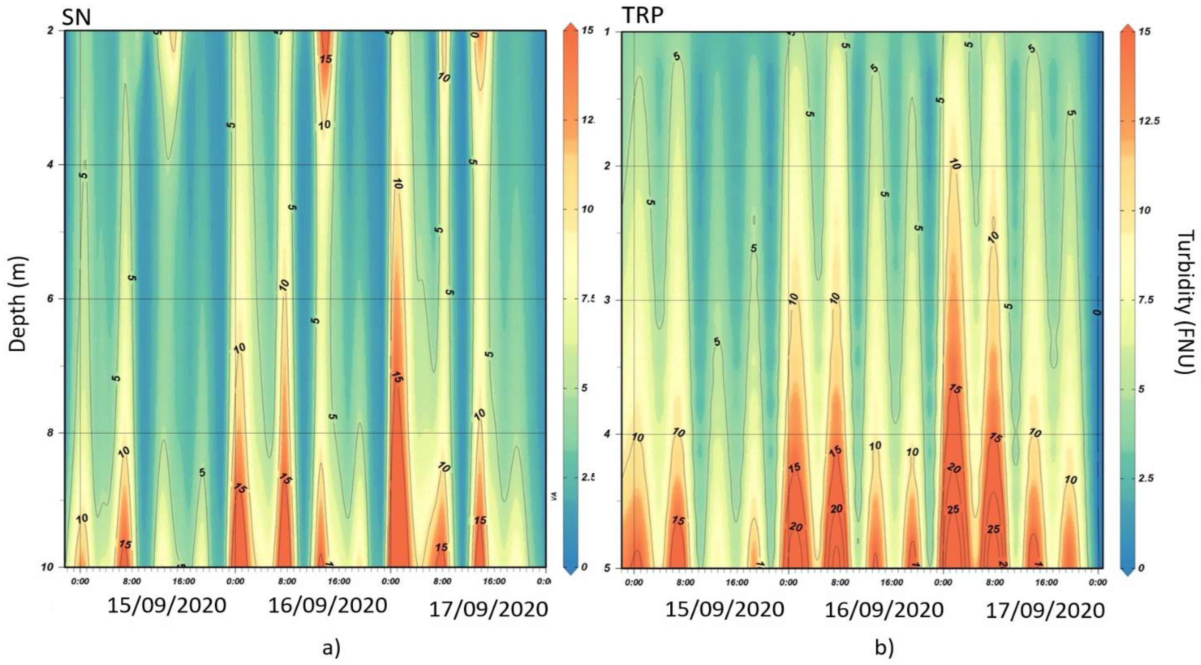
4.5. Long-Term Dataset of In Situ Turbidity, Hydrodynamics and Meteo-Marine Forcing
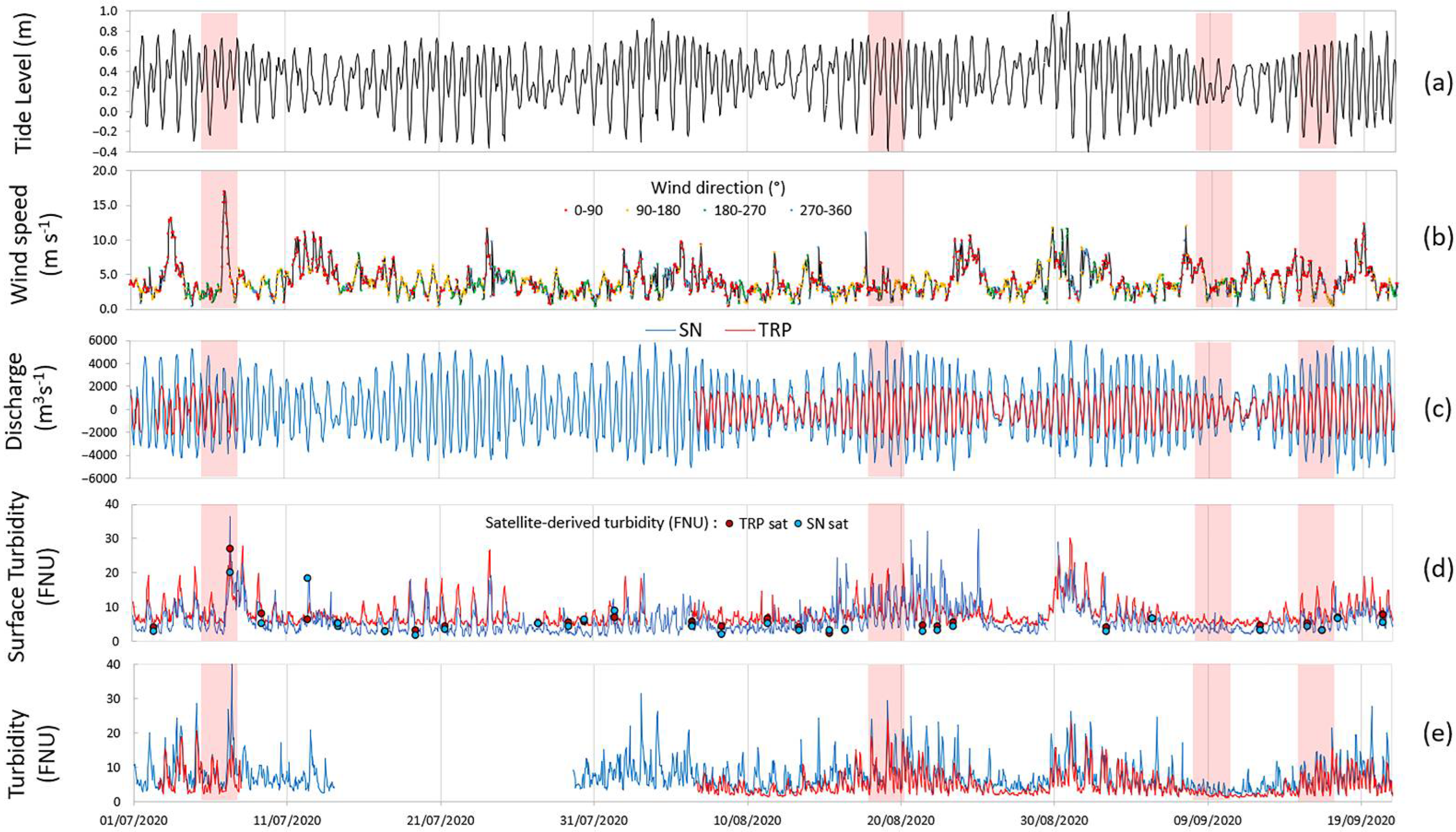
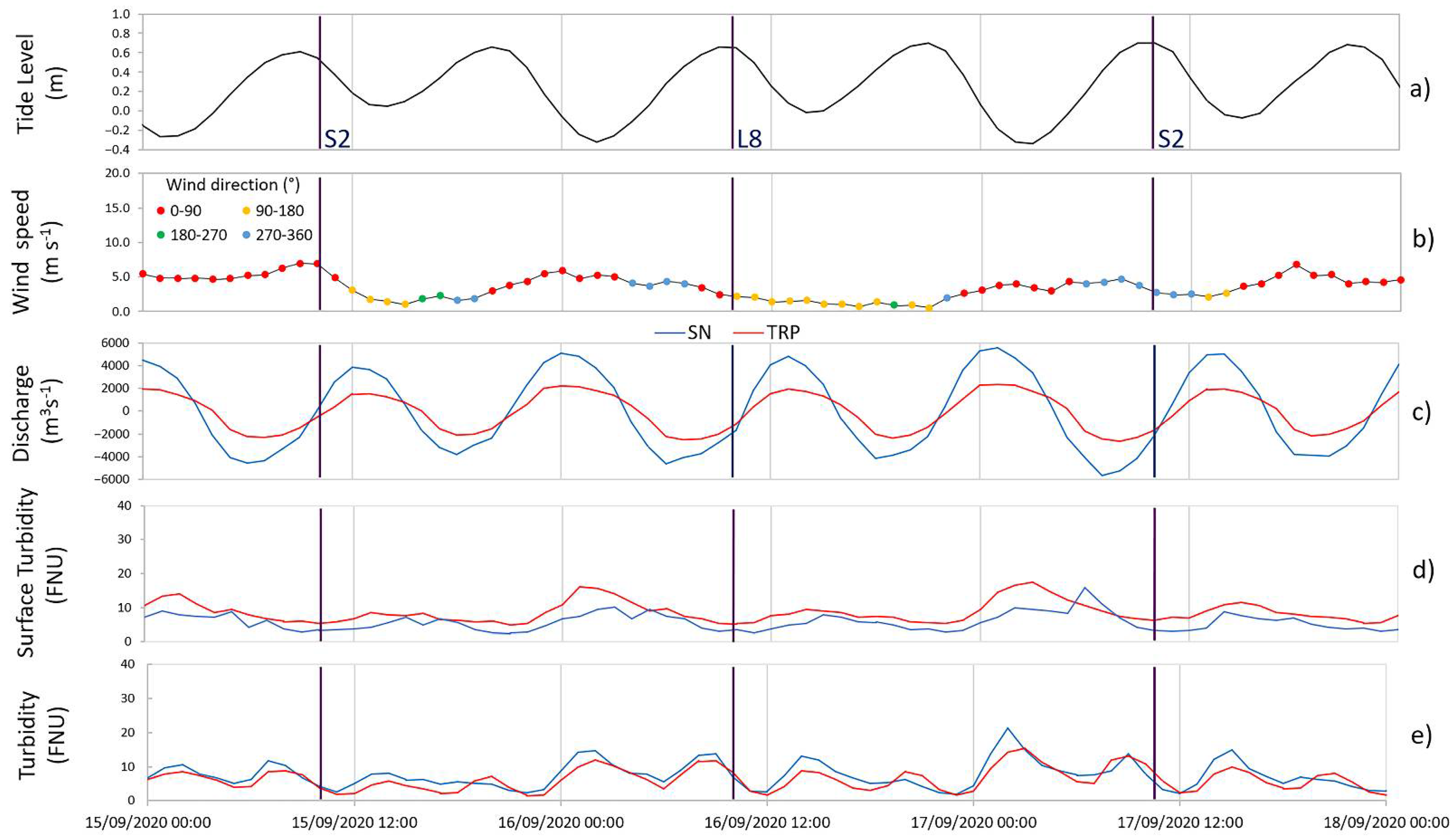
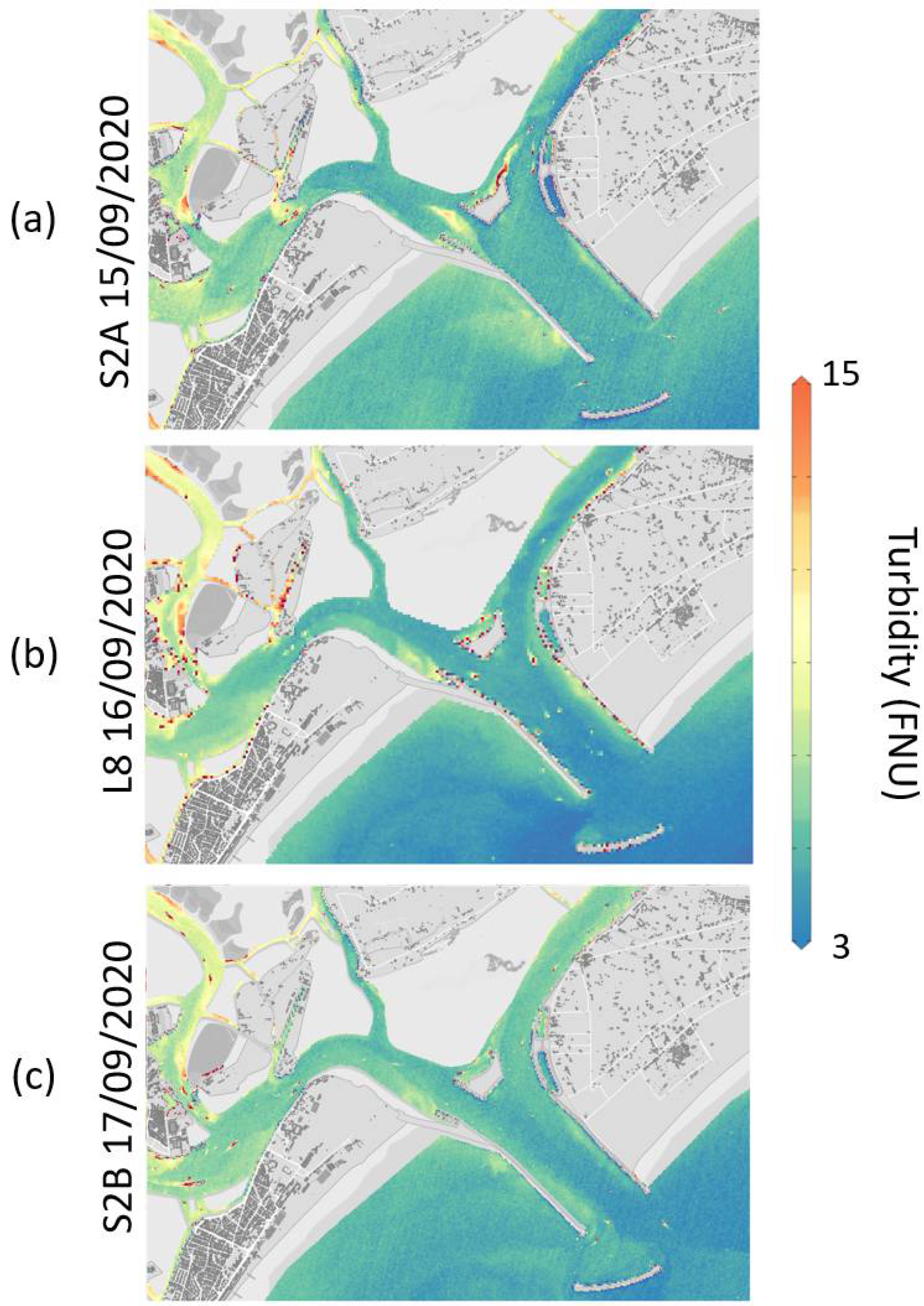
4.6. Demonstration Case of 15–17 September 2020. Test of the Integration of the Analyzed Variables
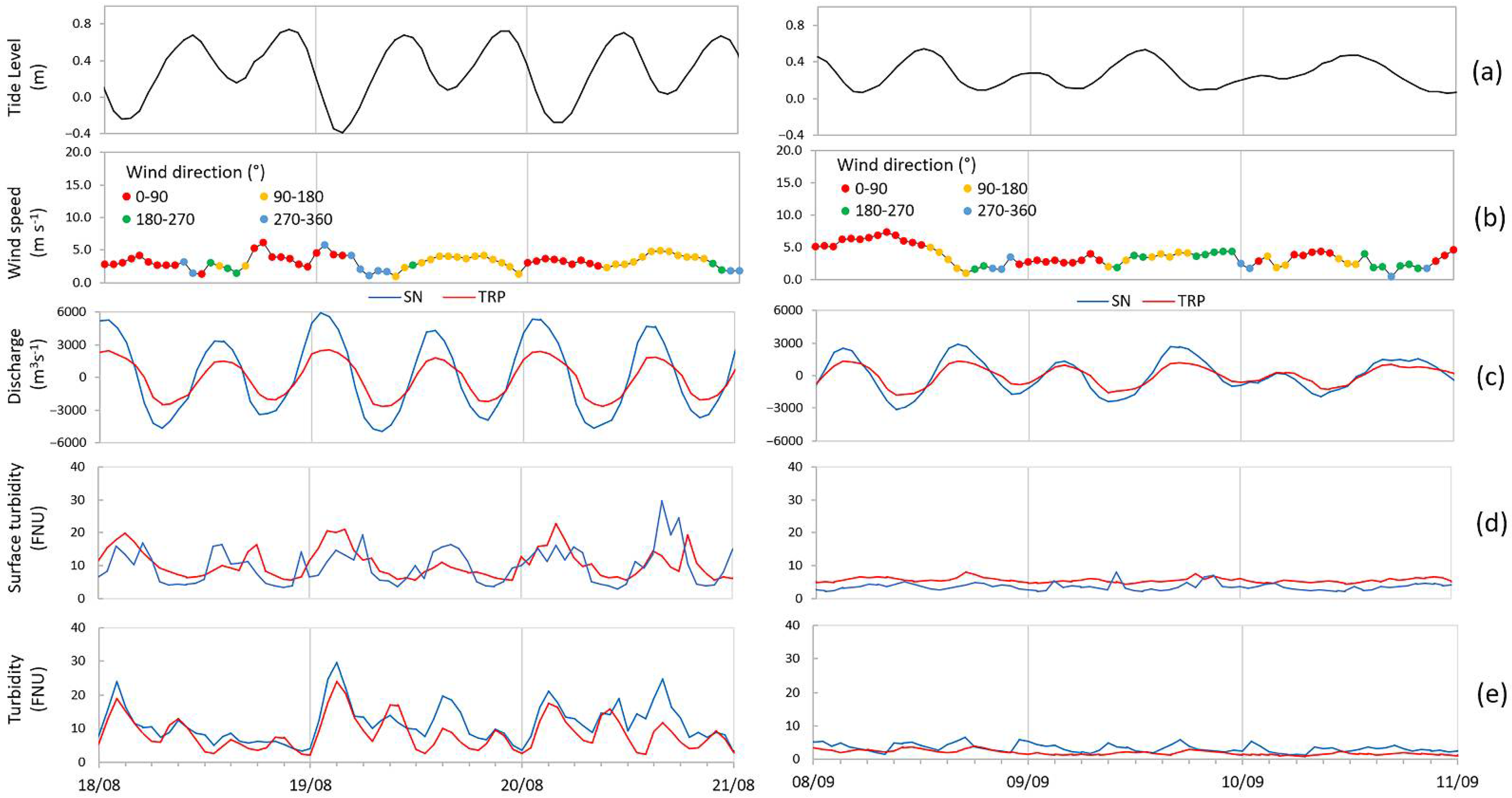
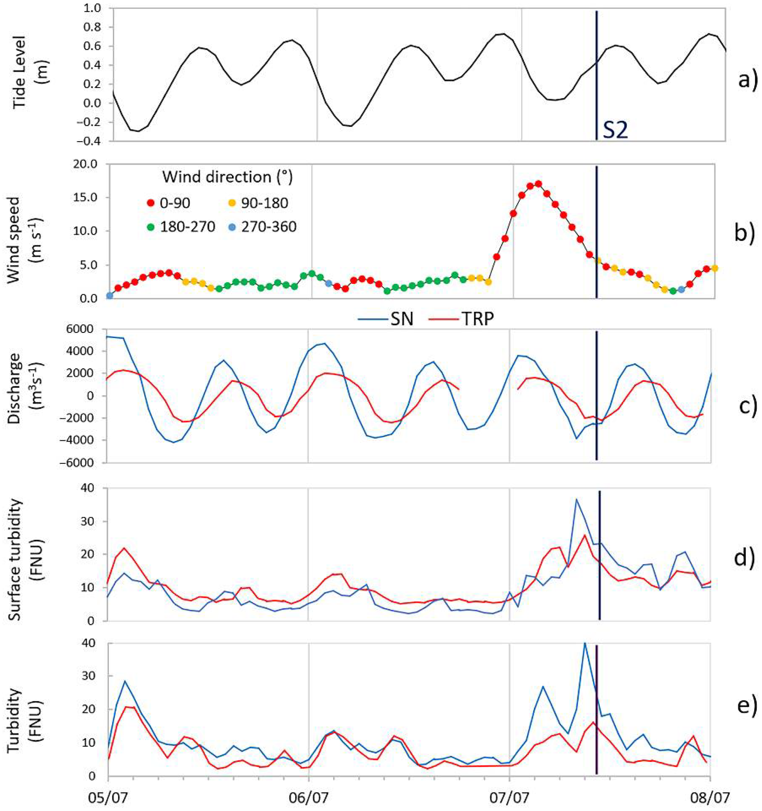
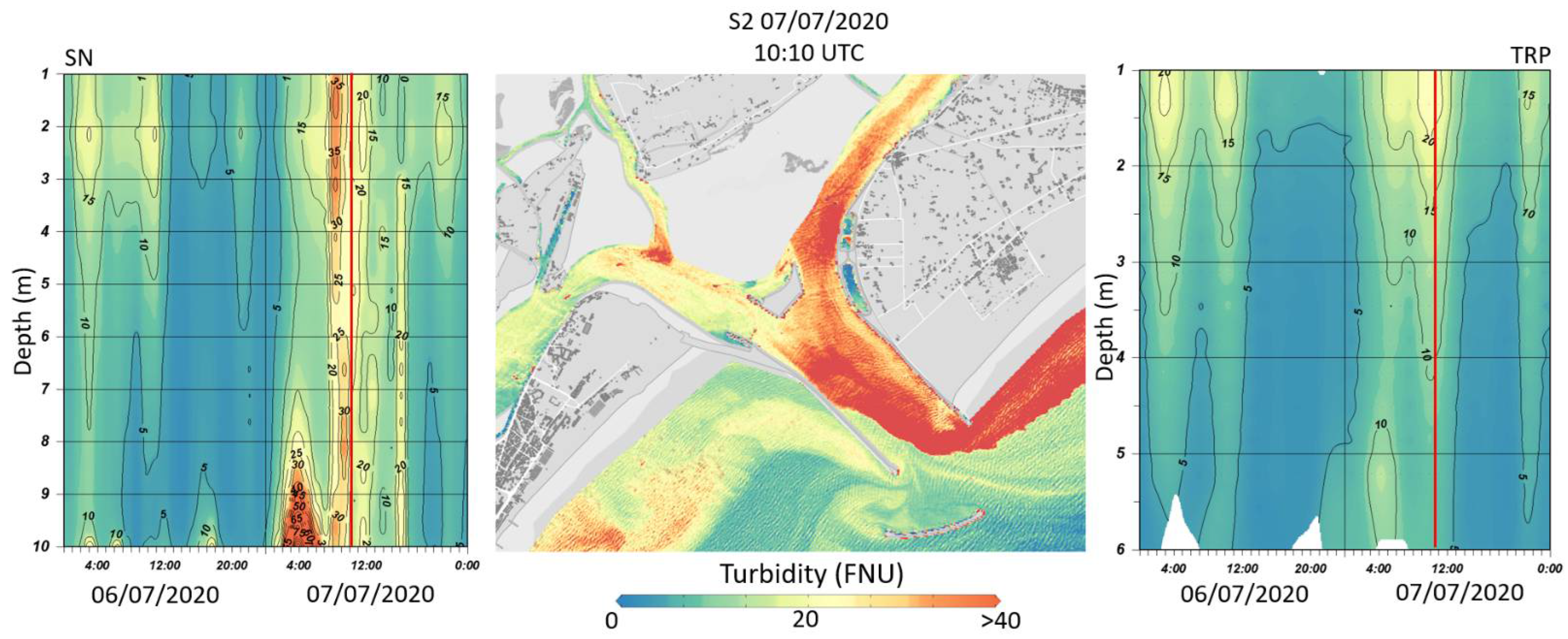
4.7. Application of the Implemented Methodology to the 5–7 July 2020 Meteo-Marine Event
5. Conclusions
Supplementary Materials
Author Contributions
Funding
Data Availability Statement
Acknowledgments
Conflicts of Interest
References
- Cohen, J.E.; Small, C.; Mellinger, A.; Gallup, J.; Sachs, J. Estimates of Coastal Populations. Science 1997, 278, 1209–1213. [Google Scholar] [CrossRef]
- Fletcher, C.A.; Spencer, T. Flooding and Environmental Challenges for Venice and Its Lagoon: State of Knowledge; Cambridge University Press: Cambridge, UK, 2005; ISBN 978-0-521-84046-0. [Google Scholar]
- Gonenc, I.E.; Wolflin, J.P. Coastal Lagoons: Ecosystem Processes and Modeling for Sustainable Use and Development; CRC Press: New York, NY, USA, 2004; ISBN 978-0-429-20926-0. [Google Scholar]
- Newton, A.; Brito, A.C.; Icely, J.D.; Derolez, V.; Clara, I.; Angus, S.; Schernewski, G.; Inácio, M.; Lillebø, A.I.; Sousa, A.I.; et al. Assessing, Quantifying and Valuing the Ecosystem Services of Coastal Lagoons. J. Nat. Conserv. 2018, 44, 50–65. [Google Scholar] [CrossRef]
- Anthony, A.; Atwood, J.; August, P.; Byron, C.; Cobb, S.; Foster, C.; Fry, C.; Gold, A.; Hagos, K.; Heffner, L.; et al. Coastal Lagoons and Climate Change: Ecological and Social Ramifications in U.S. Atlantic and Gulf Coast Ecosystems. Ecol. Soc. 2009, 14, 29. [Google Scholar] [CrossRef]
- Brown, K.M.; Tims, J.L.; Erwin, R.M.; Richmond, M.E. Changes in the nesting populations of colonial waterbirds in Jamaica Bay wildlife refuge, New York, 1974–1998. Northeast. Nat. 2001, 8, 275–292. [Google Scholar] [CrossRef]
- Cai, F.; Su, X.; Liu, J.; Li, B.; Lei, G. Coastal Erosion in China under the Condition of Global Climate Change and Measures for Its Prevention. Prog. Nat. Sci. 2009, 19, 415–426. [Google Scholar] [CrossRef]
- Besset, M.; Anthony, E.J.; Brunier, G.; Dussouillez, P. Shoreline Change of the Mekong River Delta along the Southern Part of the South China Sea Coast Using Satellite Image Analysis (1973–2014). Géomorphologie Relief Process. Environ. 2016, 22, 137–146. [Google Scholar] [CrossRef]
- Zhang, Y.; Hou, X. Characteristics of Coastline Changes on Southeast Asia Islands from 2000 to 2015. Remote Sens. 2020, 12, 519. [Google Scholar] [CrossRef] [Green Version]
- Zanchettin, D.; Bruni, S.; Raicich, F.; Lionello, P.; Adloff, F.; Androsov, A.; Antonioli, F.; Artale, V.; Carminati, E.; Ferrarin, C.; et al. Sea-Level Rise in Venice: Historic and Future Trends (Review Article). Nat. Hazards Earth Syst. Sci. 2021, 21, 2643–2678. [Google Scholar] [CrossRef]
- Lionello, P.; Nicholls, R.J.; Umgiesser, G.; Zanchettin, D. Venice Flooding and Sea Level: Past Evolution, Present Issues, and Future Projections (Introduction to the Special Issue). Nat. Hazards Earth Syst. Sci. 2021, 21, 2633–2641. [Google Scholar] [CrossRef]
- Thorne, P.D.; Hardcastle, P.J.; Flatt, D.; Humphery, J.D. On the Use of Acoustics for Measuring Shallow Water Suspended Sediment Processes. IEEE J. Ocean. Eng. 1994, 19, 48–57. [Google Scholar] [CrossRef]
- Holdaway, G.P.; Thorne, P.D.; Flatt, D.; Jones, S.E.; Prandle, D. Comparison between ADCP and Transmissometer Measurements of Suspended Sediment Concentration. Cont. Shelf Res. 1999, 19, 421–441. [Google Scholar] [CrossRef]
- Gartner, J.W. Estimating Suspended Solids Concentrations from Backscatter Intensity Measured by Acoustic Doppler Current Profiler in San Francisco Bay, California. Mar. Geol. 2004, 211, 169–187. [Google Scholar] [CrossRef]
- Kirwan, M.L.; Megonigal, J.P. Tidal Wetland Stability in the Face of Human Impacts and Sea-Level Rise. Nature 2013, 504, 53–60. [Google Scholar] [CrossRef] [PubMed]
- Solidoro, C.; Bandelj, V.; Bernardi, F.; Camatti, E.; Ciavatta, S.; Cossarini, G.; Facca, C.; Franzoi, P.; Libralato, S.; Canu, D.; et al. Response of the Venice Lagoon Ecosystem to Natural and Anthropogenic Pressures over the Last 50 Years. In Coastal Lagoons; Kennish, M., Paerl, H., Eds.; Marine Science; CRC Press: Boca Raton, FL, USA, 2010; Volume 20103358, pp. 483–511. ISBN 978-1-4200-8830-4. [Google Scholar]
- Newton, A.; Icely, J.; Cristina, S.; Brito, A.; Cardoso, A.C.; Colijn, F.; Riva, S.D.; Gertz, F.; Hansen, J.W.; Holmer, M.; et al. An Overview of Ecological Status, Vulnerability and Future Perspectives of European Large Shallow, Semi-Enclosed Coastal Systems, Lagoons and Transitional Waters. Estuar. Coast. Shelf Sci. 2014, 140, 95–122. [Google Scholar] [CrossRef]
- Ackroyd, P. Venice: Pure City; Talese, N.A., Ed.; Doubleday: New York, NY, USA, 2009. [Google Scholar]
- Ferrarin, C.; Cucco, A.; Umgiesser, G.; Bellafiore, D.; Amos, C.L. Modelling Fluxes of Water and Sediment between Venice Lagoon and the Sea. Cont. Shelf Res. 2010, 30, 904–914. [Google Scholar] [CrossRef] [Green Version]
- Ferrarin, C.; Tomasin, A.; Bajo, M.; Petrizzo, A.; Umgiesser, G. Tidal Changes in a Heavily Modified Coastal Wetland. Cont. Shelf Res. 2015, 101, 22–33. [Google Scholar] [CrossRef]
- Tognin, D.; D’Alpaos, A.; Marani, M.; Carniello, L. Marsh resilience to sea-level rise reduced by storm-surge barriers in the Venice Lagoon. Nat. Geosci. 2021, 14, 906–911. [Google Scholar] [CrossRef]
- Gačić, M.; Mancero Mosquera, I.; Kovačević, V.; Mazzoldi, A.; Cardin, V.; Arena, F.; Gelsi, G. Temporal Variations of Water Flow between the Venetian Lagoon and the Open Sea. J. Mar. Syst. 2004, 51, 33–47. [Google Scholar] [CrossRef]
- Bianchi, F.; Ravagnan, E.; Acri, F.; Bernardi-Aubry, F.; Boldrin, A.; Camatti, E.; Cassin, D.; Turchetto, M. Variability and Fluxes of Hydrology, Nutrients and Particulate Matter between the Venice Lagoon and the Adriatic Sea. Preliminary Results (Years 2001–2002). J. Mar. Syst. 2004, 51, 49–64. [Google Scholar] [CrossRef]
- Bellafiore, D.; Umgiesser, G.; Cucco, A. Modeling the Water Exchanges between the Venice Lagoon and the Adriatic Sea. Ocean Dyn. 2008, 58, 397–413. [Google Scholar] [CrossRef]
- Defendi, V.; Kovačević, V.; Arena, F.; Zaggia, L. Estimating Sediment Transport from Acoustic Measurements in the Venice Lagoon Inlets. Cont. Shelf Res. 2010, 30, 883–893. [Google Scholar] [CrossRef]
- Gačić, M.; Kovačević, V.; Mazzoldi, A.; Paduan, J.; Arena, F.; Mosquera, I.M.; Gelsi, G.; Arcari, G. Measuring Water Exchange between the Venetian Lagoon and the Open Sea. Eos Trans. Am. Geophys. Union 2002, 83, 217–222. [Google Scholar] [CrossRef]
- Tambroni, N.; Seminara, G. Are Inlets Responsible for the Morphological Degradation of Venice Lagoon? J. Geophys. Res. Earth Surf. 2006, 111. [Google Scholar] [CrossRef] [Green Version]
- Umgiesser, G.; De Pascalis, F.; Ferrarin, C.; Amos, C.L. A Model of Sand Transport in Treporti Channel: Northern Venice Lagoon. Ocean Dyn. 2006, 56, 339. [Google Scholar] [CrossRef]
- Carniello, L.; D’Alpaos, A.; Defina, A. Modeling wind waves and tidal flows in shallow micro-tidal basins. Estuar. Coast. Shelf Sci. 2011, 92, 263–276. [Google Scholar] [CrossRef]
- Madricardo, F.; Foglini, F.; Kruss, A.; Ferrarin, C.; Pizzeghello, N.M.; Murri, C.; Rossi, M.; Bajo, M.; Bellafiore, D.; Campiani, E.; et al. High Resolution Multibeam and Hydrodynamic Datasets of Tidal Channels and Inlets of the Venice Lagoon. Sci. Data 2017, 4, 170121. [Google Scholar] [CrossRef] [Green Version]
- Toso, C.; Madricardo, F.; Molinaroli, E.; Fogarin, S.; Kruss, A.; Petrizzo, A.; Pizzeghello, N.M.; Sinapi, L.; Trincardi, F. Tidal Inlet Seafloor Changes Induced by Recently Built Hard Structures. PLoS ONE 2019, 14, e0223240. [Google Scholar] [CrossRef]
- Ghezzo, M.; Guerzoni, S.; Cucco, A.; Umgiesser, G. Changes in Venice Lagoon Dynamics Due to Construction of Mobile Barriers. Coast. Eng. 2010, 57, 694–708. [Google Scholar] [CrossRef] [Green Version]
- Volpe, V.; Silvestri, S.; Marani, M. Remote Sensing Retrieval of Suspended Sediment Concentration in Shallow Waters. Remote Sens. Environ. 2011, 115, 44–54. [Google Scholar] [CrossRef]
- Carniello, L.; Silvestri, S.; Marani, M.; D’Alpaos, A.; Volpe, V.; Defina, A. Sediment Dynamics in Shallow Tidal Basins: In Situ Observations, Satellite Retrievals, and Numerical Modeling in the Venice Lagoon. J. Geophys. Res. Earth Surf. 2014, 119, 802–815. [Google Scholar] [CrossRef] [Green Version]
- Braga, F.; Zaggia, L.; Bellafiore, D.; Bresciani, M.; Giardino, C.; Lorenzetti, G.; Maicu, F.; Manzo, C.; Riminucci, F.; Ravaioli, M.; et al. Mapping Turbidity Patterns in the Po River Prodelta Using Multi-Temporal Landsat 8 Imagery. Estuar. Coast. Shelf Sci. 2017, 198, 555–567. [Google Scholar] [CrossRef]
- Cucco, A.; Umgiesser, G. Modeling the Venice Lagoon Residence Time. Ecol. Model. 2006, 193, 34–51. [Google Scholar] [CrossRef]
- Helsby, R. Sand Transport in Northern Venice Lagoon through the Tidal Inlet of Lido. Ph.D. Thesis, University of Southampton, Southampton, UK, 2008. [Google Scholar]
- Cosoli, S.; Mazzoldi, A.; Gačić, M. Validation of Surface Current Measurements in the Northern Adriatic Sea from High-Frequency Radars. J. Atmos. Ocean. Technol. 2010, 27, 908–919. [Google Scholar] [CrossRef]
- Zuliani, A.; Zaggia, L.; Collavini, F.; Zonta, R. Freshwater Discharge from the Drainage Basin to the Venice Lagoon (Italy). Environ. Int. 2005, 31, 929–938. [Google Scholar] [CrossRef]
- Collavini, F.; Bettiol, C.; Zaggia, L.; Zonta, R. Pollutant Loads from the Drainage Basin to the Venice Lagoon (Italy). Environ. Int. 2005, 31, 939–947. [Google Scholar] [CrossRef]
- Simpson, M.R.; Bland, R. Methods for Accurate Estimation of Net Discharge in a Tidal Channel. IEEE J. Ocean. Eng. 2000, 25, 437–445. [Google Scholar] [CrossRef]
- Brando, V.E.; Braga, F.; Zaggia, L.; Giardino, C.; Bresciani, M.; Matta, E.; Bellafiore, D.; Ferrarin, C.; Maicu, F.; Benetazzo, A.; et al. High-Resolution Satellite Turbidity and Sea Surface Temperature Observations of River Plume Interactions during a Significant Flood Event. Ocean Sci. 2015, 11, 909–920. [Google Scholar] [CrossRef] [Green Version]
- Braga, F.; Scarpa, G.M.; Brando, V.E.; Manfè, G.; Zaggia, L. COVID-19 Lockdown Measures Reveal Human Impact on Water Transparency in the Venice Lagoon. Sci. Total Environ. 2020, 736, 139612. [Google Scholar] [CrossRef]
- Pahlevan, N.; Chittimalli, S.K.; Balasubramanian, S.V.; Vellucci, V. Sentinel-2/Landsat 8 Product Consistency and Implications for Monitoring Aquatic Systems. Remote Sens. Environ. 2019, 220, 19–29. [Google Scholar] [CrossRef]
- Vanhellemont, Q.; Ruddick, K. Atmospheric Correction of Metre-Scale Optical Satellite Data for Inland and Coastal Water Applications. Remote Sens. Environ. 2018, 216, 586–597. [Google Scholar] [CrossRef]
- Vanhellemont, Q. Adaptation of the Dark Spectrum Fitting Atmospheric Correction for Aquatic Applications of the Landsat and Sentinel-2 Archives. Remote Sens. Environ. 2019, 225, 175–192. [Google Scholar] [CrossRef]
- Dogliotti, A.I.; Ruddick, K.G.; Nechad, B.; Doxaran, D.; Knaeps, E. A Single Algorithm to Retrieve Turbidity from Remotely-Sensed Data in All Coastal and Estuarine Waters. Remote Sens. Environ. 2015, 156, 157–168. [Google Scholar] [CrossRef] [Green Version]
- Nechad, B.; Ruddick, K.G.; Park, Y. Calibration and validation of a generic multisensor algorithm for mapping of total suspended matter in turbid waters. Remote Sens. Environ. 2010, 114, 854–866. [Google Scholar] [CrossRef]
- Barsi, J.A.; Barker, J.L.; Schott, J.R. An Atmospheric Correction Parameter Calculator for a Single Thermal Band Earth-Sensing Instrument. In Proceedings of the IGARSS 2003 IEEE International Geoscience and Remote Sensing Symposium (IEEE Cat. No. 03CH37477), Toulouse, France, 21–25 July 2003; Volume 5, pp. 3014–3016. [Google Scholar]
- Braga, F.; Ciani, D.; Colella, S.; Organelli, E.; Pitarch, J.; Brando, V.E.; Bresciani, M.; Concha, J.A.; Giardino, C.; Scarpa, G.M.; et al. COVID-19 lockdown effects on a coastal marine environment: Disentangling perception versus reality. Sci. Total Environ. 2022, 817, 153002. [Google Scholar] [CrossRef] [PubMed]
- Molinaroli, E.; Guerzoni, S.; Sarretta, A.; Masiol, M.; Pistolato, M. Thirty-Year Changes (1970 to 2000) in Bathymetry and Sediment Texture Recorded in the Lagoon of Venice Sub-Basins, Italy. Mar. Geol. 2009, 258, 115–125. [Google Scholar] [CrossRef] [Green Version]


Publisher’s Note: MDPI stays neutral with regard to jurisdictional claims in published maps and institutional affiliations. |
© 2022 by the authors. Licensee MDPI, Basel, Switzerland. This article is an open access article distributed under the terms and conditions of the Creative Commons Attribution (CC BY) license (https://creativecommons.org/licenses/by/4.0/).
Share and Cite
Scarpa, G.M.; Braga, F.; Manfè, G.; Lorenzetti, G.; Zaggia, L. Towards an Integrated Observational System to Investigate Sediment Transport in the Tidal Inlets of the Lagoon of Venice. Remote Sens. 2022, 14, 3371. https://doi.org/10.3390/rs14143371
Scarpa GM, Braga F, Manfè G, Lorenzetti G, Zaggia L. Towards an Integrated Observational System to Investigate Sediment Transport in the Tidal Inlets of the Lagoon of Venice. Remote Sensing. 2022; 14(14):3371. https://doi.org/10.3390/rs14143371
Chicago/Turabian StyleScarpa, Gian Marco, Federica Braga, Giorgia Manfè, Giuliano Lorenzetti, and Luca Zaggia. 2022. "Towards an Integrated Observational System to Investigate Sediment Transport in the Tidal Inlets of the Lagoon of Venice" Remote Sensing 14, no. 14: 3371. https://doi.org/10.3390/rs14143371