Transformer-Based Global Zenith Tropospheric Delay Forecasting Model

Abstract

Zenith tropospheric delay (ZTD) plays an important role in high-precision global navigation satellite system (GNSS) positioning and meteorology. At present, commonly used ZTD forecasting models comprise empirical, meteorological parameter, and neural network models. The empirical model can only fit approximate periodic variations, and its accuracy is relatively low. The accuracy of the meteorological parameter model depends heavily on the accuracy of the meteorological parameters. The recurrent neural network (RNN) is suitable for short-term series data prediction, but for long-term series, the ZTD prediction accuracy is clearly reduced. Long short-term memory (LSTM) has superior forecasting accuracy for long-term ZTD series; however, the LSTM model is complex, cannot be parallelized, and is time-consuming. In this study, we propose a novel ZTD time-series forecasting utilizing transformer-based machine-learning methods that are popular in natural language processing (NLP) and forecasting global ZTD, the training parameters provided by the global geodetic observing system (GGOS). The proposed transformer model leverages self-attention mechanisms by encoder and decoder modules to learn complex patterns and dynamics from long ZTD time series. The numeric results showed that the root mean square error (RMSE) of the forecasting ZTD results were 1.8 cm and mean bias, STD, MAE, and R 0.0, 1.7, 1.3, and 0.95, respectively, which is superior to that of the LSTM, RNN, convolutional neural network (CNN), and GPT3 series models. We investigated the global distribution of these accuracy indicators, and the results demonstrated that the accuracy in continents was superior to maritime space transformer ZTD forecasting model accuracy at high latitudes superior to that at low latitude. In addition to the overall accuracy improvement, the proposed transformer ZTD forecast model also mitigates the accuracy variations in space and time, thereby guaranteeing high accuracy globally. This study provides a novel method to estimate the ZTD, which could potentially contribute to precise GNSS positioning and meteorology.

1. Introduction

When global navigation satellite system (GNSS) signals travel through the troposphere, they experience a delay and bending due to tropospheric refraction, resulting in tropospheric delay errors [1]. The error can be mapped to zenith direction to obtain zenith tropospheric delay (ZTD) by a mapping function [2,3]. Prior ZTD as tropospheric augmentation information is crucial for GNSS precise point positioning (PPP) and real-time kinematic (RTK) high-precision atmospheric corrections [4]. ZTD can be divided into zenith hydrostatic delay (ZHD) and zenith wet delay (ZWD). The ZWD component can be converted into precipitable water vapor (PWV) by weighted mean temperature (Tm) and is a crucial parameter in meteorological applications [5].

ZTD can be obtained by the following approaches: (1) estimated as an unknown parameter in GNSS data processing [6]; (2) constructed by meteorological parameter models [7]; (3) calculated by empirical models [8]; (4) measured by sounding stations [9]; and (5) implemented by machine-learning methods [10]. At present, the most accurate and reliable approach is the measured ZTD, but the cost of monitoring stations is high and the spatial distribution uneven, which makes it difficult to obtain measured high spatial resolution ZTD [11].

Many scholars have proposed a large number of classic models, such as the Hopfield model [12], Black model [13], EGNOS (European Geostationary Navigation Overlay System) model [14], and Saastamoinen model [15]. These models have slight differences in different situations, but their accuracy is reliable. The UNB series model [16,17] uses tables to write such parameters as temperature, air pressure, and relative temperature into a list of latitude and annual days. The tropospheric delay at sea level is calculated, followed by the calculation of the tropospheric zenith delay at the station. UNB series models do not require the measured meteorological parameters.

With decades of data accumulation, machine-learning methods have begun to stand out among the other methods owing to their excellent processing capabilities for massive ZTD data [18]. Therefore, it is important to model and forecast ZTD using machine-learning methods to improve the forecast duration and accuracy.

Machine-learning methods leverage ground-measured ZTD data to learn trends and patterns, and deep learning approaches based on convolutional neural networks (CNNs) [19] and recurrent neural networks (RNN) [20] have been developed to model ZTD time-series data. Long short-term memory (LSTM) is an implementation of RNN that can effectively represent time series with long-term patterns, and has been utilized in many fields, including meteorology, network traffic, and air pollution forecasting [21,22,23,24,25,26]. Zhu et al. developed multi-channel LSTM neural networks to learn from different types of inputs and used an attention layer to associate the model output with the input sequence to further improve the forecast accuracy [27]. Zhang et al. established an hourly ZTD model using GPS-derived ZTD products by independent component analysis (ICA) and principal component analysis (PCA), and conducted short-time-span regional ZTD forecasting model using a long short-term memory (LSTM) neural network. Their results showed that ICA was superior to PCA, and the 24-h ZTD forecasting root mean square error (RMSE) was 13.3 cm [28]. These sequence-aligned models are natural choices for modeling time-series data. However, due to “gradient vanishing and exploding” problems, hard to parallel in RNNs, and the limits of convolutional filters, these methods have limitations in modeling long-term and complex relations in the sequence data [29]. Obtaining precipitation information quickly and accurately has attracted increasing attention from meteorological researchers. In recent years, Li et al. explored a transformer-based architecture, proposed convolutional layers for local processing, and employed a sparse attention mechanism to increase the receptive field size during prediction. The results showed that their model memory cost only O(L(log L)²) and improved forecasting accuracy for strong long-term dependence time series [30].

In this study, we investigated self-attention by producing queries (Q), keys (K), and values (V) incorporated with an attention mechanism to establish a transformer ZTD forecasting model, thereby improving the forecasting accuracy for ZTD time series with granularity and strong long-term dependence under a constrained memory budget.

2. Materials and Methods

In this section, we introduce the transformer model, analyze the global distribution of ZTD-derived VMF stations (VMF-ZTD) provided by GGOS, eliminate outliers with Grubbs’s test, fill the ZTD data gap by K nearest neighbor algorithm, and verify the accuracy between VMF-ZTD and the ZTD-derived IGS (IGS-ZTD). VMF-ZTD time-series data from 2008 to 2019 and 2020 were employed to train and test the transformer forecast model. The schematic methodology for establishing the transformer ZTD forecasting model is shown in Figure 1.

2.1. Transformer Model

At present, the transformer model has achieved great success in the fields of image, text, audio, and time-series data processing [31,32]. In this study, we established a transformer ZTD forecasting model that follows the original transformer architecture [33], which consists of two modules: an encoder and decoder. The structure of the transformer ZTD forecasting model is illustrated in Figure 2.

The transformer-encoder modules include a ZTD input embedding layer, positional encoding layer, and three encoder layers with identical structures. The ZTDs were mapped to a d_model-dimension vector through a fully connected layer in the input embedding layer, which is crucial for the transformer ZTD forecasting model to leverage the multi-head attention mechanism. The positional encoding layer encodes ZTDs by the element-wise addition of an input vector with a positional encoding vector. The output vector was transferred to three encoder layers. Each encoder layer includes two sub-layers: a feed-forward sub-layer and a self-attention sub-layer, with each sub-layer followed by a normalized operation. The transformer encoder outputs a d_model-dimension vector, which was transferred to the transformer-decoder modules [34].

The transformer-decoder module layers are similar to those of the encoder. The decoder’s first input ZTD sample point is the last encoder input ZTD sample point. In addition to the two sub-layers, another sub-layer was designed to leverage the self-attention mechanisms over the encoder output. The output layer maps the output of the last decoder layer to the predicted ZTD time sequence. The look-ahead mask and one-position offset layer were designed between the decoder input and target ZTD output to ensure that the predicted ZTD depended only on the previous ZTD [35].

2.2. Study Area and Data

We employed global VMF stations provided by the Global Geodetic Observing System (GGOS) to investigate, analyze, and forecast ZTD. There were 505 stations in total, and their spatial distribution is shown in Figure 3.

Figure 3 shows the 505 VMF stations (light green circles) and 402 IGS stations (dark green circles). There are 142 collocated stations (red triangles), according to the min-heap algorithm [36]. The condition was that the distance between VMF stations and IGS stations less than 2 km was used as a threshold to identify collocated stations. We employed those collocated station to verify the outer accuracy of the VMF-ZTD [37].

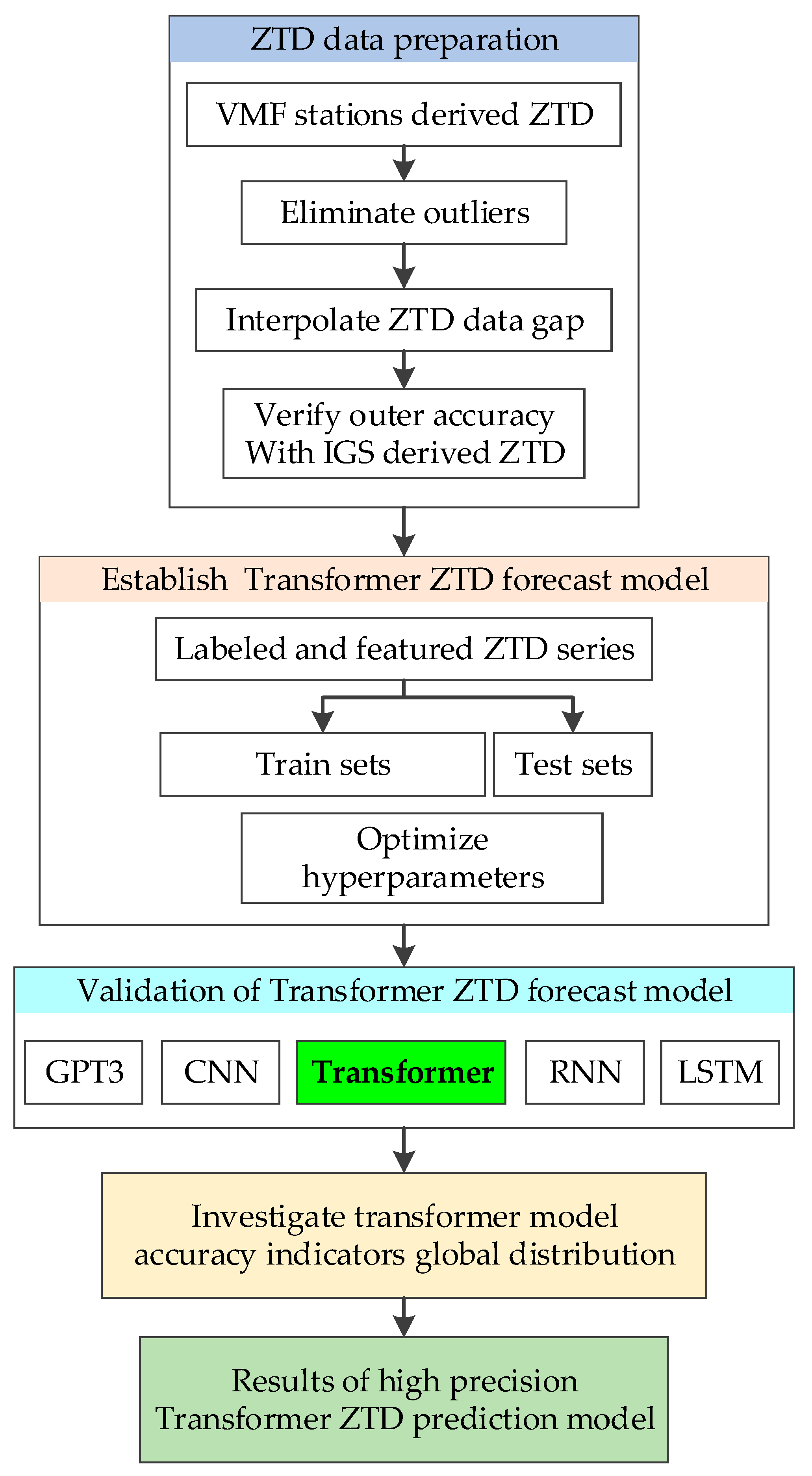
2.3. Data Preprocessing

We employed the VMF-derived ZTD (VMF-ZTD) from 2008 to 2020 from the Global Geodetic Observing System (GGOS) repository (https://vmf.geo.tuwien.ac.at/trop_products/GNSS/VMF3/VMF3_OP/, accessed on 4 October 2021) to investigate the accuracy of VMF-ZTD, taking IGS-provided ZTD (IGS-ZTD; ftp://cddis.gsfc.nasa.gov/pub/gps/data, accessed on 5 October 2021) as reference. The time resolutions of VMF-ZTD and IGS-derived ZTD were 6 h and 5 min, respectively. We standardized the sampling time of VMF-ZTD and IGS-ZTD according to Equation (1) to validate the outer accuracy of VMF-ZTD and IGS-ZTD, where DOY is the day of the year and HOD the hour of the day. We resampled IGS-ZTD into 6 h to keep the two derived ZTD sampling times consistent.

Due to the absence of the ZTD data itself and the elimination of obvious outliers, the time-series data of ZTD were discontinuous. The outliers were eliminated using Grubbs’s test criteria [38], and the ZTD data gap was interpolated by the K nearest neighbor algorithm. The K nearest neighbor algorithm filled missing ZTD data according to the mean value of the K nearest ZTD data points around the gap. The basic principle of the K nearest neighbor algorithm is to calculate K and nearest ZTD observation data based on Euclidean distance and estimate the missing data by the inverse weighting of the distance [39]. The input parameters for train the K nearest neighbor model are the ZTD after eliminated the outliers and corresponding time t, calculated by Equation (1). We found that the ZTD series were discontinuous and unevenly spaced. Complete time series were fed into the trained K nearest neighbor model, and the output parameters interpolated ZTD. The K nearest neighbor model was implemented with the knn-regression module in Scikit-learn (https://scikit-learn.org/stable/modules/neighbors.html?highlight=knn-regression, accessed on 8 October 2021).

Table 1. The ZTD outer accuracy (cm) between IGS and VMF collocated stations.

Bias	STD	MAE	RMSE	R
−0.08	1.00	0.96	1.19	0.95

shows the outer accuracy between VMF-ZTD and IGS-ZTD at DOY 336–366, 2020. Figure 4 shows a comparison of the accuracy of the radar map. Figure 5 shows the time-series trends.

$$t=\frac{DOY}{365.25}+\frac{HOD}{365.25\times 24}$$

(1)

Figure 4 and Table 1 indicate that there was high outer accuracy of VMF-ZTD and IGS-ZTD. Bias/R/STD/MAE/RMSE was −0.08/0.95/1.00/0.96/1.19 cm, respectively, calculated by Equations (2)–(5). All collocated station ZTD data statistic showed that the overall outer accuracy between VMF-ZTD and IGS-ZTD was very high. We randomly selected three stations from all the collocated stations, taking ABPO (longitude: 47.2292°E, latitude: 18.98169°S, height: 1553 m), RAMO (longitude: 34.76313889°E, latitude: 30.59761°S, height: 886.8 m), and TWTF (longitude: 121.1645°E, latitude: 24.9535°S, height: 201.5 m) stations as examples, to investigate the detailed variation trend between the two ZTD data sources.

Figure 5 shows the time-series trend comparison between VMF-ZTD and IGS-ZTD. The RMSE between VMF-ZTD and IGS-ZTD was about 1.2 cm, and their time-series trends were almost in step with each other. The latitude of ABPO, RAMO, and TWTF IGS stations was 18.98169°S, 30.59761°S, and 24.9535°S, respectively. They were all in low latitudes of the southern hemisphere. The elevation of the three IGS stations gradually decreased from 1553 to 201 m. Figure 5 implies the ZTD increasing from 2.08 to 2.34 m. ABPO and RAMO located in the west hemisphere, TWTF in the east hemisphere, and the ZTD trend were consistent. The above analysis results show that VMF-ZTD was very close to IGS-ZTD, which ensured the reliability of the data source employed in this study, so we used VMF-ZTD for further analysis and research.

Figure 6a shows the distribution of annual mean VMF-ZTD in 2020 for all of the stations around the world. Figure 6b shows the global elevation distribution. It implies that the higher altitude corresponded to larger ZTD and the lower altitude to smaller ZTD, and that means with small ZTD were in high latitudes and large ZTD in low latitudes. The ZTD is symmetrically distributed in the northern and southern hemispheres. The maximum ZTD value was located at the equator, reaching 2.6 m, the minimum value located in the Qinghai–Tibet Plateau (1.5 m), and the global mean ZTD in 2020 was 2.128 m. From the perspective of Figure 6a, the west coasts of South America and North America and the east coast of Africa have smaller ZTDs, while comparing these with Figure 6b demonstrated that these places had higher altitude, which further explains the higher altitude having the smaller ZTD.

Figure 7 shows ABPO, RAMO, and TWTF stations’ ZTD time series from 2008 to 2020, VMF-ZTD displays obvious annual periodic characteristics. We employed the model expression construct period-ZTD, (orange curve). The period model can only fit the general change trend of VMF-ZTD, but the details can’t be expressed accurately. In order to improve ZTD prediction accuracy, we used a transformer model to further study the ZTD time series.

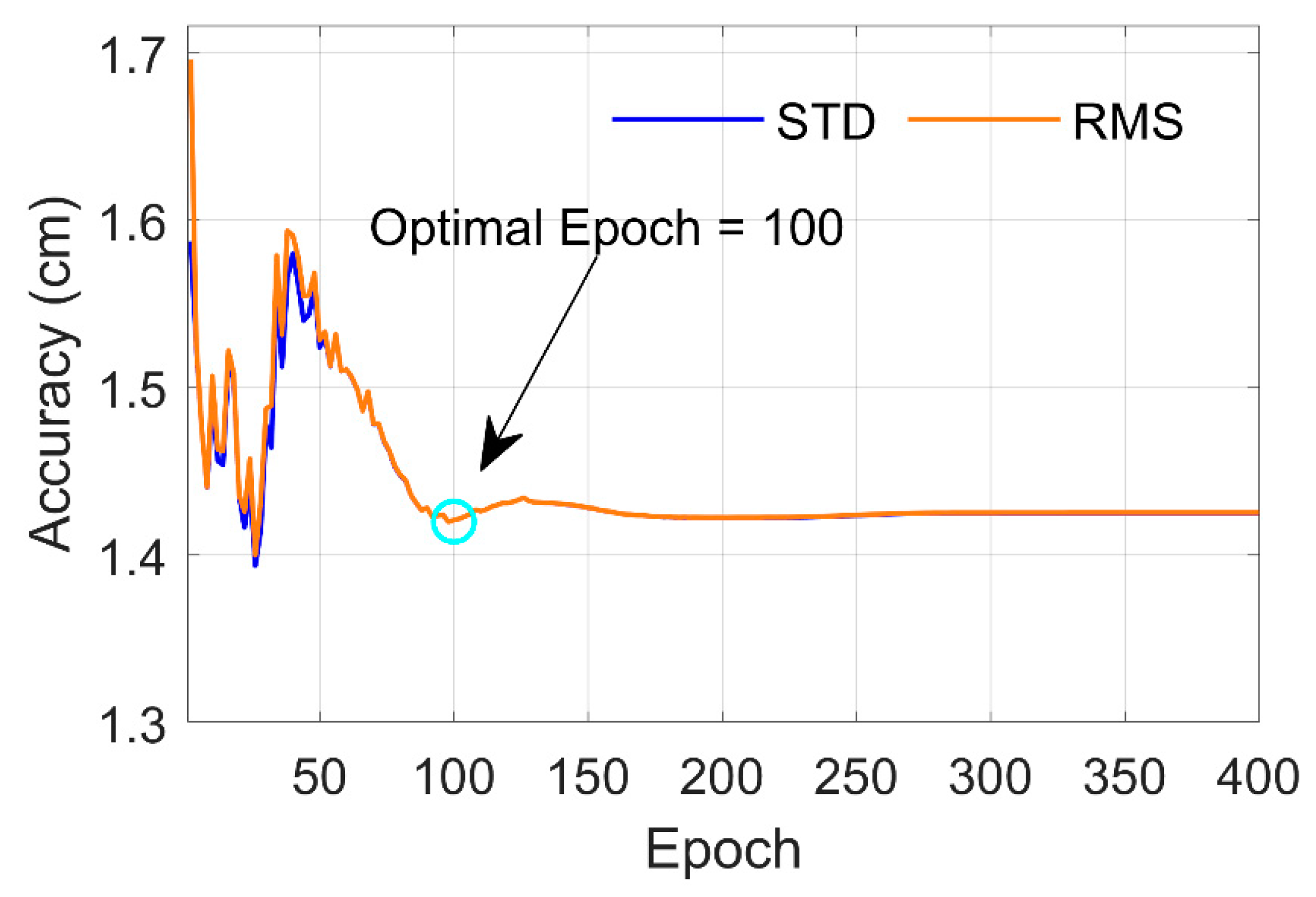
2.4. Construction of Transformer ZTD Forecast Model

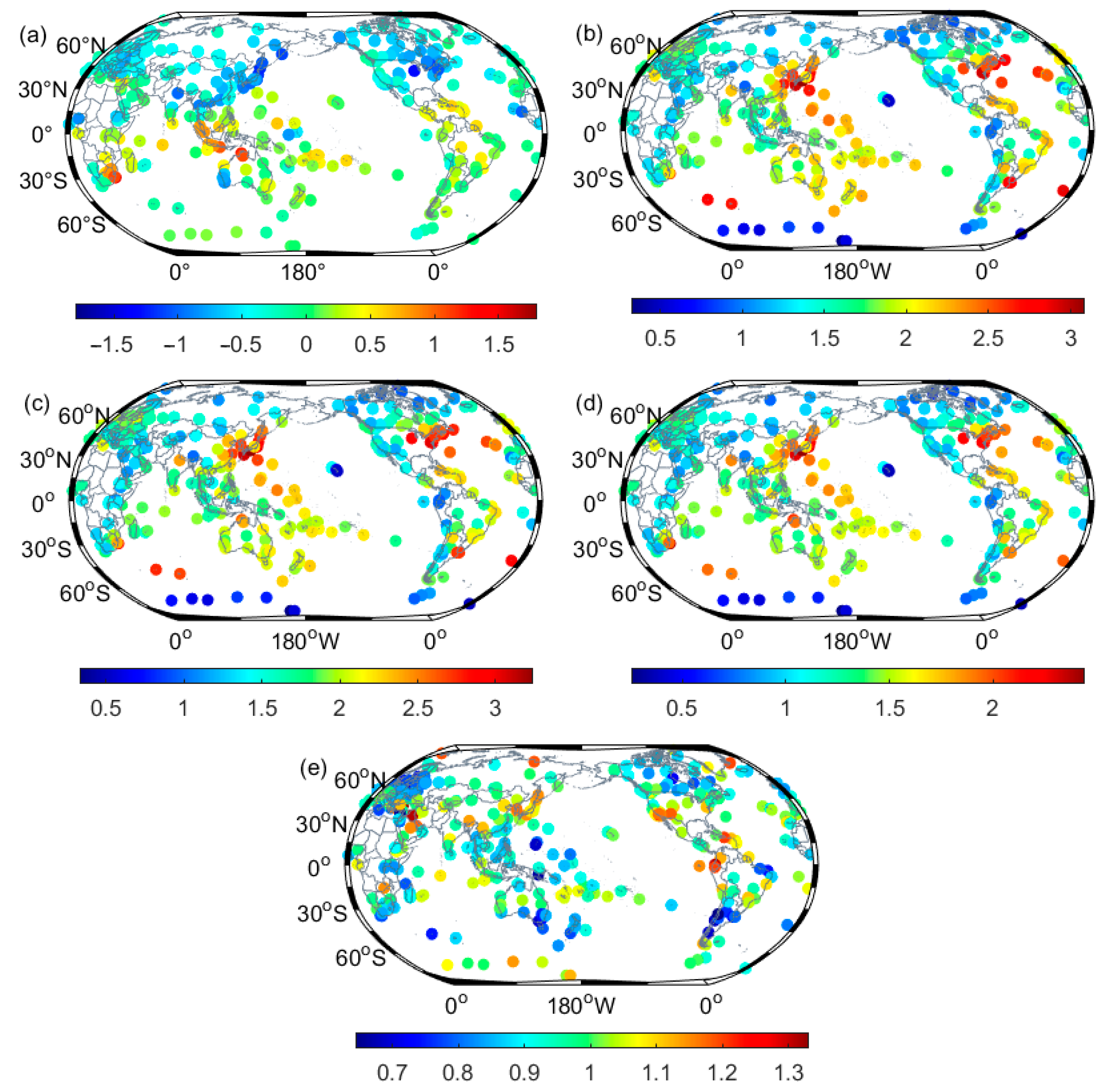
The transformer uses recurrent layers for local processing and interpretable self-attention layers for long-term dependence. The transformer selects relevant features and a series of gating layers to suppress unnecessary components, enabling outstanding performance in the ZTD time-series forecasts [40,41].

Figure 8 shows the fixed-length sliding time window. We employed a sliding window to build X, Y pairs to obtain ZTD training and validation samples with featured and labeled ZTD data sets. The featured and labeled ZTD are the previous and next observations, respectively. The ZTD data sets were scaled with maximum and minimum ZTD training samples before the sliding window operation.

In a typical training step, we trained the transformer ZTD forecasting model to predict four future ZTDs from 10 training ZTD data points. This means that given the encoder input ($x_1,x_2,\cdots ,x_{10}$) and decoder input ($x_{10},\cdots ,x_{13}$), the decoder aims to output ($x_{11},\cdots ,x_{14}$). A look-ahead mask is applied to ensure that attention is only applied to prior ZTD data points to target the ZTD by the transformer model. When predicting the target ($x_{11},x_{12}$), the mask ensures that the attention weights are only on ($x_{10},x_{11}$), and the decoder does not leak information about $x_{12}$ and $x_{13}$ from the decoder input. A mini-batch of 64 was used for training.

The model epoch was determined by calculating the STD and RMSE through cross-validation. Figure 9 shows that when the training epoch of the transformer model is 100, the model accuracy tends to stabilize, so we set 100 as the training epoch during training.

The featured and labeled ZTD samples from 2008 to 2020 were used to establish the transformer ZTD forecasting model. The ZTD samples from 2008 to 2019 (approximately 91.7%) were used to train the model, whereas the rest of the data (approximately 8.3%) as the test set were applied to verify the effectiveness of the transformer ZTD forecasting model. We employed the Adam optimizer and the learning rate was set to 0.01, applying dropout techniques for each of the three types of sub-layers in the encoder and decoder: the self-attention sub-layer, the feed-forward sub-layer, and the normalization sub-layer. The dropout rate of each sub-layer was 0.02.

It took 11 h 56 min to train the transformer model on a supercomputing system at the Supercomputing Center of Wuhan University. The supercomputing system was equipped with 2580.175 MHz, 20-core processor-containing CPU and 128 GB RAM.

The GPT model can obtain the temperature and pressure near Earth’s surface using only the coordinate information of the station and the day of the year (DOY). It can also model the variation period of the parameters. At present, the GPT series models have gradually evolved to GPT2, GPT2w, and GPT3 from the original GPT model. GPT2w introduces the vertical lapse rate of water-vapor pressure based on the GPT2 model to improve the accuracy of ZWD, while GPT3 introduces a gradient model based on GPT2w to further optimize the model. The GPT3 model improves the mapping function coefficients and overcomes the mapping function error caused by the low zenith angle [3,42].

The CNN is a biologically inspired type of deep neural network (DNN) and has been successfully applied in classification and regression. CNN is a type of feed-forward neural network that includes convolution computation and a depth structure. It is a representative deep-learning algorithm. CNN has the ability of representation learning and can use shift-invariant classification of input information according to hierarchical structure [43]. CNN consists of a series of convolutional layers that connect the output to local regions in the input by computing a dot product at each two point. This structure allows the model to learn filters that can recognize specific patterns in the input data.

The RNN is a type of recursive neural network that takes sequence data as input, recursion in the evolution direction of the sequence, and all nodes (loop units) are connected in a chain. It has the characteristics of memory, parameter sharing, and Turing completeness, so it has certain advantages in learning the nonlinear characteristics of sequences. Recurrent neural networks have been applied in natural language processing (NLP), such as speech recognition, language modeling, an machine translation, and has also been used in various time-series forecasting.

The LSTM is a kind of time-recurrent neural network that is specially designed to solve the long-term dependence problem of general RNN. All RNNs have a chain form of repetitive neural network module. In a standard RNN, this repetitive structural module has only a very simple structure, such as a tanh layer [44]. LSTM is the earliest proposed RNN gating algorithm, and its corresponding recurrent unit, the LSTM unit, contains three gates: input gate, forget gate, and output gate. In contrast to the recursive computation established by the RNN for the cell state, the three gates establish a self-loop for the internal state of the LSTM unit. Specifically, the input gate determines the update of the internal state by the input of the current time step and the cell state of the previous time step; the forgetting gate determines the update of the internal state of the previous time step to the internal state of the current time step; and the output gate determines the update of the internal state to the cell state.

3. Results

In this section, we demonstrate the precision indicators of the transformer model, we employed the GPT3 and popular machine-learning models to compare and verify the transformer model accuracy in predicting ZTD, and analyzed the variation in model accuracy on a global scale.

In the same vein, we employed GPT3 models, CNN, RNN, and LSTM neural network models from the training set and test set of the transformer model to forecast the ZTD sequences in 2020 to compare the accuracy of the transformer model.

Figure 10 shows the predicted ZTD and observed ZTD test results among the different models. The GPT3 and CNN models had lower accuracy. RNN and LSTM neural network accuracy was superior to the GPT3 and CNN models, but they were difficult to make parallel, resulting in time-consuming training. The transformer showed the optimal accuracy compared to other models, and its training speed was faster than that of the RNN and LSTM.

We calculated the transformer model precision indicators (bias, STD, RMSE, MAE, R). The equations for the indicators are as follows: (1)–(4), where N refers to the number of samples, $ZT{D}_i^{pre}$ is the ZTD value output from the transformer models, and $ZT{D}_i^{obs}$ is the observed VMF-ZTD value as reference. $\overline{ZT{D}_i^{obs}}$ and $\overline{ZT{D}_i^{pre}}$ are the mean values of $ZT{D}_i^{obs}$ and $ZT{D}_i^{pre}$, respectively. Bias reflects the degree of deviation between the ZTD predicted value and the observed value in a certain time period. STD is the dispersion of the distribution between the predicted and observed ZTD values. RMSE indicates the deviation between the predicted value and the observed value. MAE reflects the actual situation of ZTD prediction error. R is the coefficient of determination, which reflects the approximation of the model results compared to the sample data.

The numeric results showed that the transformer model global bias ranged from −1.3 to 1.5 cm, and the mean bias was approximately 0.0 cm. The STD ranged from 0.3 to 3.1 cm, mean STD was 1.7 cm, MAE ranged from 0.2 to 2.4 cm, and mean MAE was 1.3 cm. The RMSE ranged from 0.3 to 3.2 cm, and the mean RMSE was 1.8 cm. R ranged from 0.91 to 0.97, and mean R was 0.95. Figure 11 and

Table 2. Transformer accuracy indicators (cm) and time spent.

Model	Bias	STD	MAE	RMSE	R	Time Spent
GPT3	0.0	3.7	3.0	3.7	0.62	-
CNN	0.0	3.5	2.8	3.5	0.85	5 h 27 min
RNN	0.0	2.1	1.5	2.1	0.93	8 d 7 h 12 min
LSTM	0.0	1.8	1.4	1.9	0.94	10 d 4 h 53 min
Transformer	0.0	1.7	1.3	1.8	0.95	11 h 56 min

show the statistical accuracy of the different models, indicating that the GPT3 and CNN models had larger RMSE and STD, and the bias of these models was approximately the same. The transformer model had the largest R value, up to 0.95, followed by LSTM (0.94), while the GPT3 model had the lowest R value, only 0.62. The statistical results show that the RMSE of the transformer improved by 5.3%, 14.3%, 48.6%, and 51.3% compared with LSTM, RNN, CNN, and GPT3, respectively. Similarly, R improved by 34.7%, 10.5%, 2.1%, and 2.1%, respectively. Both STD and MAE were improved accordingly.

$$Bias=\frac{1}{N}{\displaystyle {\sum }_{i=1}^N(ZT{D}_i^{pre}-ZT{D}_i^{obs})}$$

(2)

$$STD=\sqrt{\frac{1}{N}{\displaystyle {\sum }_{i=1}^N{(ZT{D}_i^{pre}-ZT{D}_i^{obs}-Bias)}^2}}$$

(3)

$$RMSE=\sqrt{\frac{1}{N}{\displaystyle {\sum }_{i=1}^N{(ZT{D}_i^{pre}-ZT{D}_i^{obs})}^2}}$$

(4)

$$R=\frac{{\displaystyle {\sum }_{i=1}^N(ZT{D}_i^{pre}-\overline{ZT{D}_i^{pre}})}(ZT{D}_i^{obs}-\overline{ZT{D}_i^{obs}})}{\sqrt{{\displaystyle {\sum }_{i=1}^N{(ZT{D}_i^{pre}-\overline{ZT{D}_i^{pre}})}^2}{\displaystyle {\sum }_{i=1}^N{(ZT{D}_i^{obs}-\overline{ZT{D}_i^{obs}})}^2}}}$$

(5)

The time spent on training the models is presented in Table 2. The calculation speed of the GPT3 model was the fastest. The transformer and CNN models could be parallelized, and the training speed was significantly better than that of the RNN and LSTM models, which were difficult to parallelize, and training took a lot of time.

4. Discussion

To further analyze the temporal variations in transformer model accuracy, we investigated the global spatial distribution. Figure 12 shows the global distribution of the transformer model precision indicators. It suggests that transformer bias, STD, and RMSE in inland areas were superior to those in ocean areas. The transformer forecasting model accuracy indicators at high latitudes were larger than at low latitudes and larger on land than over the sea. The west coast of South America and North America had better accuracy. The minimum bias was distributed in the east coast of Asia and east coast of North America. The maximum bias was distributed around equatorial land. The minimum STD was distributed in the polar regions, and the maximum STD was distributed along the west coast of the Pacific and Atlantic Oceans. The RMSE and MAE had similar distributions to the STD.

The proposed transformer ZTD forecasting model had the best accuracy at the South and North Poles and the Qinghai–Tibet Plateau. Accuracy for the North and South Poles was mainly due to the inactive troposphere. The perfect accuracy for the Qinghai–Tibet Plateau was mainly due to altitude. The statistical results showed that the RMSE values for the Antarctic, Arctic, and Qinghai–Tibet Plateau regions varied from 0.25 to 0.32, 0.4 to 1.1 and 0.419 to 1.614 cm, respectively. The numeric results showed that the transformer model exhibited good prediction accuracy, demonstrating the rationality of the modeling. In addition, the training time and attention mechanism of the transformer model can be further optimized, and it is expected that subsequent scholars can make a leap in this respect.

5. Conclusions

In this paper, we proposed a novel transformer ZTD forecasting model. The VMF stations provided by GGOS during 2008–2020 were used to train and validate the effectiveness of the proposed model. A transformer, which is popular in NLP (natural language processing), was adopted to study the ZTD time-series data. Several classic neural network models (RNN, CNN, LSTM) and GPT3 models were used to compare the accuracy of the transformer ZTD forecast model.

The numeric results showed that the RMSE of the transformer was 1.8 cm and was improved by 5.3%, 14.3%, 48.6%, and 51.3% compared to the LSTM, RNN, CNN, and GPT3, respectively, further indicating that the proposed transformer ZTD forecast model yields state-of-the-art forecasting results. Through the variation in accuracy on a global scale, it was demonstrated that the transformer ZTD forecast model mitigates the accuracy variations in space and time, guaranteeing high accuracy across the board. This study provides a novel method to estimate ZTD, and could potentially contribute to precise GNSS positioning and meteorology.

References

1. Rózsa, S.; Ambrus, B.; Juni, I.; Ober, P.B.; Mile, M. An advanced residual error model for tropospheric delay estimation. GPS Solut. 2020, 24, 1–15. [Google Scholar] [CrossRef]
2. Böhm, J.; Möller, G.; Schindelegger, M.; Pain, G.; Weber, R. Development of an improved empirical model for slant delays in the troposphere (GPT2w). GPS Solut. 2015, 19, 433–441. [Google Scholar] [CrossRef] [Green Version]
3. Landskron, D.; Böhm, J. VMF3/GPT3: Refined discrete and empirical troposphere mapping functions. J. Geod. 2018, 92, 349–360. [Google Scholar] [CrossRef]
4. Wabbena, G.; Schmitz, M.; Bagge, A. PPP-RTK: Precise point positioning using state-space representation in RTK networks. In Proceedings of the 18th International Technical Meeting of the Satellite Division of the Institute of Navigation (ION GNSS 2005), Long Beach, CA, USA, 13–16 September 2005; pp. 2584–2594. [Google Scholar]
5. Sun, Z.; Zhang, B.; Yao, Y. Improving the estimation of weighted mean temperature in China using machine learning methods. Remote Sens. 2021, 13, 1016. [Google Scholar] [CrossRef]
6. Shi, J.; Xu, C.; Guo, J.; Gao, Y. Local troposphere augmentation for real-time precise point positioning. Earth Planets Space 2014, 66, 1–13. [Google Scholar] [CrossRef] [Green Version]
7. Douša, J.; Eliaš, M.; Václavovic, P.; Eben, K.; Krč, P. A two-stage tropospheric correction model combining data from GNSS and numerical weather model. GPS Solut. 2018, 22, 1–13. [Google Scholar] [CrossRef]
8. Lagler, K.; Schindelegger, M.; Böhm, J.; Krásná, H.; Nilsson, T. GPT2: Empirical slant delay model for radio space geodetic techniques. Geophys. Res. Lett. 2013, 40, 1069–1073. [Google Scholar] [CrossRef] [PubMed] [Green Version]
9. Jiang, P.; Ye, S.; Chen, D.; Liu, Y.; Xia, P. Retrieving Precipitable Water Vapor Data Using GPS Zenith Delays and Global Reanalysis Data in China. Remote Sens. 2016, 8, 389. [Google Scholar] [CrossRef] [Green Version]
10. Osah, S.; Acheampong, A.A.; Fosu, C.; Dadzie, I. Deep learning model for predicting daily IGS zenith tropospheric delays in West Africa using TensorFlow and Keras. Adv. Space Res. 2021, 68, 1243–1262. [Google Scholar] [CrossRef]
11. Yao, Y.; Xu, C.; Shi, J.; Cao, N.; Zhang, B.; Yang, J. ITG: A new global GNSS tropospheric correction model. Sci. Rep. 2015, 5, 1–9. [Google Scholar] [CrossRef] [Green Version]
12. Hopfield, H.S. Two-quartic tropospheric refractivity profile for correcting satellite data. J. Geophys. Res. 1969, 74, 4487–4499. [Google Scholar] [CrossRef]
13. Black, H.D. An easily implemented algorithm for the tropospheric range correction. J. Geophys. Res. Solid Earth 1978, 83, 1825–1828. [Google Scholar] [CrossRef]
14. Penna, N.; Dodson, A.; Chen, W. Assessment of EGNOS tropospheric correction model. J. Navig. 2001, 54, 37–55. [Google Scholar] [CrossRef] [Green Version]
15. Saastamoinen, J. Contributions to the theory of atmospheric refraction. Bull. Géodésique (1946–1975) 1972, 105, 279–298. [Google Scholar] [CrossRef]
16. Collins, J.P.; Langley, R.B. A Tropospheric Delay Model for the User of the Wide Area Augmentation System; Department of Geodesy and Geomatics Engineering, University of New Brunswick: Fredericton, NB, Canada, 1997. [Google Scholar]
17. Leandro, R.; Santos, M.; Langley, R. UNB neutral atmosphere models: Development and performance. In Proceedings of the 2006 National Technical Meeting of the Institute of Navigation, Monterey, CA, USA, 18–20 January 2006; pp. 564–573. [Google Scholar]
18. Shamshiri, R.; Motagh, M.; Nahavandchi, H.; Haghshenas Haghighi, M.; Hoseini, M. Improving tropospheric corrections on large-scale Sentinel-1 interferograms using a machine learning approach for integration with GNSS-derived zenith total delay (ZTD). Remote Sens. Environ. 2020, 239, 111608. [Google Scholar] [CrossRef]
19. Anantrasirichai, N.; Biggs, J.; Albino, F.; Bull, D. A deep learning approach to detecting volcano deformation from satellite imagery using synthetic datasets. Remote Sens. Environ. 2019, 230, 111179. [Google Scholar] [CrossRef] [Green Version]
20. Gao, W.; Gao, J.; Yang, L.; Wang, M.; Yao, W. A Novel Modeling Strategy of Weighted Mean Temperature in China Using RNN and LSTM. Remote Sens. 2021, 13, 3004. [Google Scholar] [CrossRef]
21. Miao, K.; Han, T.; Yao, Y.; Lu, H.; Chen, P.; Wang, B.; Zhang, J. Application of LSTM for short term fog forecasting based on meteorological elements. Neurocomputing 2020, 408, 285–291. [Google Scholar] [CrossRef]
22. Wu, Q.; Guan, F.; Lv, C.; Huang, Y. Ultra-short-term multi-step wind power forecasting based on CNN-LSTM. IET Renew. Power Gener. 2021, 15, 1019–1029. [Google Scholar] [CrossRef]
23. Tsai, Y.T.; Zeng, Y.R.; Chang, Y.S. Air pollution forecasting using RNN with LSTM. In Proceedings of the 2018 IEEE 16th International Conference on Dependable, Autonomic and Secure Computing, 16th International Conference on Pervasive Intelligence and Computing, 4th International Conference on Big Data Intelligence and Computing and Cyber Science and Technology Congress (DASC/PiCom/DataCom/CyberSciTech), Athens, Greece, 12–15 August 2018; IEEE: Piscataway, NJ, USA, 2018; pp. 1074–1079. [Google Scholar]
24. Ma, Y.; Zhang, Z.; Ihler, A. Multi-lane short-term traffic forecasting with convolutional LSTM network. IEEE Access 2020, 8, 34629–34643. [Google Scholar] [CrossRef]
25. Yu, R.; Li, Y.; Shahabi, C.; Demiryurek, U.; Liu, Y. Deep learning: A generic approach for extreme condition traffic forecasting. In Proceedings of the 2017 SIAM International Conference on Data Mining, Houston, TX, USA, 27–29 April 2017; Society for Industrial and Applied Mathematics: Philadelphia, PA, USA, 2017; pp. 777–785. [Google Scholar]
26. Dalgkitsis, A.; Louta, M.; Karetsos, G.T. Traffic forecasting in cellular networks using the LSTM RNN. In Proceedings of the 22nd Pan-Hellenic Conference on Informatics, Athens, Greece, 29 November–1 December 2018; pp. 28–33. [Google Scholar]
27. Zhu, X.; Fu, B.; Yang, Y.; Ma, Y.; Hao, J.; Chen, S.; Liu, S.; Li, T.; Liu, S.; Guo, W.; et al. Attention-based recurrent neural network for influenza epidemic prediction. BMC Bioinform. 2019, 20, 575. [Google Scholar] [CrossRef] [PubMed]
28. Zhang, Q.; Li, F.; Zhang, S.; Li, W. Modeling and Forecasting the GPS Zenith Troposphere Delay in West Antarctica Based on Different Blind Source Separation Methods and Deep Learning. Sensors 2020, 20, 2343. [Google Scholar] [CrossRef] [PubMed] [Green Version]
29. Sherstinsky, A. Fundamentals of Recurrent Neural Network (RNN) and Long Short-Term Memory (LSTM) Network. Phys. D Nonlinear Phenom. 2020, 404, 132306. [Google Scholar] [CrossRef] [Green Version]
30. Li, S.; Jin, X.; Xuan, Y.; Zhou, X.; Chen, W.; Wang, Y.-X.; Yan, X. Enhancing the locality and breaking the memory bottleneck of transformer on time series forecasting. Adv. Neural Inf. Processing Syst. 2019, 32, 5243–5253. [Google Scholar]
31. Han, K.; Wang, Y.; Chen, H.; Chen, X.; Guo, J.; Liu, Z.; Tang, Y.; Xiao, A.; Xu, C.; Xu, Y.; et al. A survey on vision transformer. arXiv 2020, arXiv:2012.12556. [Google Scholar] [CrossRef]
32. Kondo, K.; Ishikawa, A.; Kimura, M. Sequence to sequence with attention for influenza prevalence prediction using google trends. In Proceedings of the 2019 3rd International Conference on Computational Biology and Bioinformatics, New York, NY, USA, 17–19 October 2019; pp. 1–7. [Google Scholar]
33. Vaswani, A.; Shazeer, N.; Parmar, N.; Uszkoreit, J.; Jones, L.; Gomez, A.N.; Kaiser, L.; Polosukhin, I. Attention is all you need. Adv. Neural Inf. Process. Syst. 2017, 30, 6000–6010. [Google Scholar]
34. Wu, N.; Green, B.; Ben, X.; O’Banion, S. Deep transformer models for time series forecasting: The influenza prevalence case. arXiv 2020, arXiv:2001.08317. [Google Scholar]
35. Badrinarayanan, V.; Kendall, A.; Cipolla, R. Segnet: A deep convolutional encoder-decoder architecture for image segmentation. IEEE Trans. Pattern Anal. Mach. Intell. 2017, 39, 2481–2495. [Google Scholar] [CrossRef]
36. Frederickson, G.N. An optimal algorithm for selection in a min-heap. Inf. Comput. 1993, 104, 197–214. [Google Scholar] [CrossRef] [Green Version]
37. Zhao, Q.; Yao, Y.; Yao, W.; Zhang, S. GNSS-derived PWV and comparison with radiosonde and ECMWF ERA-Interim data over mainland China. J. Atmos. Sol.-Terr. Phys. 2019, 182, 85–92. [Google Scholar] [CrossRef]
38. Grubbs, F.E. Procedures for detecting outlying observations in samples. Technometrics 1969, 11, 1–21. [Google Scholar] [CrossRef]
39. García-Laencina, P.J.; Sancho-Gómez, J.L.; Figueiras-Vidal, A.R.; Verleysen, M. K nearest neighbours with mutual information for simultaneous classification and missing data imputation. Neurocomputing 2009, 72, 1483–1493. [Google Scholar] [CrossRef]
40. Zhou, H.; Zhang, S.; Peng, J.; Zhang, S.; Li, J.; Xiong, H.; Zhang, W. Informer: Beyond efficient transformer for long sequence time-series forecasting. In Proceedings of the Thirty-Fifth AAAI Conference on Artificial Intelligence, Virtual, 2–9 February 2021. [Google Scholar]
41. Shaw, P.; Uszkoreit, J.; Vaswani, A. Self-attention with relative position representations. arXiv 2018, arXiv:1803.02155. [Google Scholar]
42. Yibin, Y.; Na, C.; Chaoqian, X.; Junjian, J. Accuracy assessment and analysis for GPT2. Acta Geod. Cartogr. Sin. 2015, 44, 726. [Google Scholar]
43. Xue, N.; Triguero, I.; Figueredo, G.P.; Landa-Silva, D. Evolving deep CNN-LSTMs for inventory time series prediction. In Proceedings of the 2019 IEEE Congress on Evolutionary Computation (CEC), Wellington, New Zealand, 10–13 June 2019; IEEE: Piscataway, NJ, USA, 2019; pp. 1517–1524. [Google Scholar]
44. Siami-Namini, S.; Tavakoli, N.; Namin, A.S. A comparison of ARIMA and LSTM in forecasting time series. In Proceedings of the 2018 17th IEEE International Conference on Machine Learning and Applications (ICMLA), Orlando, FL, USA, 17–20 December 2018; IEEE: Piscataway, NJ, USA, 2018; pp. 1394–1401. [Google Scholar]
Figure 1. Transformer ZTD forecasting model structure designed in this study.
Remotesensing 14 03335 g001
Figure 2. Transformer ZTD forecasting model structure designed in this study. The m and k denote the length of the whole ZTD sequence and the subsequence, respectively.
Remotesensing 14 03335 g002
Figure 3. Global distribution of VMF and IGS stations.
Remotesensing 14 03335 g003
Figure 4. Comparison of ZTD outer accuracy (cm) between IGS and VMF collocated stations in radar map.
Remotesensing 14 03335 g004
Figure 5. Comparison of the ZTD time-series trends at DOY 336–366, 2020 between IGS-ZTD and VMF-ZTD in collocated stations.
Remotesensing 14 03335 g005
Figure 6. (a) Global distribution of mean VMF-ZTD in 2020, (b) altitude global distribution.
Remotesensing 14 03335 g006
Figure 7. VMF-ZTD time-series trends from 2008 to 2020 at ABPO, RAMO, and TWTF stations, respectively.
Remotesensing 14 03335 g007
Figure 8. Construction of a supervised learning forecast ZTD model diagram through a fixed-length time sliding window.
Remotesensing 14 03335 g008
Figure 9. Transformer model accuracy indicators (STD and RMSE) obtained by a cross-validation variation diagram. The cyan circle marks the optimal epoch.
Remotesensing 14 03335 g009
Figure 10. Comparison of the forecasting accuracy of the different models.
Remotesensing 14 03335 g010
Figure 11. Transformer accuracy radar. Gray, orange, blue, yellow, and green represent GPT3, CNN, RNN, LSTM, and transformer models, respectively.
Remotesensing 14 03335 g011
Figure 12. Global distribution of bias: (a), STD (b), RMSE (c), MAE (d), R (e) transformer ZTD.
Remotesensing 14 03335 g012