Article

Parameter Flexible Wildfire Prediction Using Machine Learning Techniques: Forward and Inverse Modelling

1
Data Science Institute, Department of Computing, Imperial College London, London SW7 2BX, UK
2
Leverhulme Centre for Wildfires, Environment, and Society, London SW7 2AZ, UK
3
Department of Land, Air and Water Resources, University of California, Davis, CA 95616, USA
4
Georgina Mace Centre for the Living Planet, Department of Life Sciences, Imperial College London, London SW7 2BX, UK
5
Geography & Environmental Sciences, University of Reading, Reading RG6 6EU, UK
6
Department of Earth Science & Engineering, Imperial College London, London SW7 2BX, UK
*
Author to whom correspondence should be addressed.
Remote Sens. 2022, 14(13), 3228; https://doi.org/10.3390/rs14133228
Submission received: 11 May 2022 / Revised: 20 June 2022 / Accepted: 29 June 2022 / Published: 5 July 2022
(This article belongs to the Special Issue Machine Learning Techniques Applied to Geosciences and Remote Sensing)

Abstract

:
Parameter identification for wildfire forecasting models often relies on case-by-case tuning or posterior diagnosis/analysis, which can be computationally expensive due to the complexity of the forward prediction model. In this paper, we introduce an efficient parameter flexible fire prediction algorithm based on machine learning and reduced order modelling techniques. Using a training dataset generated by physics-based fire simulations, the method forecasts burned area at different time steps with a low computational cost. We then address the bottleneck of efficient parameter estimation by developing a novel inverse approach relying on data assimilation techniques (latent assimilation) in the reduced order space. The forward and the inverse modellings are tested on two recent large wildfire events in California. Satellite observations are used to validate the forward prediction approach and identify the model parameters. By combining these forward and inverse approaches, the system manages to integrate real-time observations for parameter adjustment, leading to more accurate future predictions.

Graphical Abstract

1. Introduction

There has been a significant increase in wildfire frequency in many parts of the world in the past few decades, causing losses of lives, huge economic costs and lethal effects of air pollution [1]. According to Verisks 2021 Risk Analysis [2], over four million properties in the U.S. were identified as being at high or extreme risk from wildfire. Accurate and efficient near-real time wildfire predictions, which can be used to make decisions about fire fighting strategy, are crucial for short-term fire emergency response as well as longer-term fire risk assessment [3]. However, the ability to forecast/simulate the spread of wildfires is currently limited because of the complexity of fire dynamics and the processes that control this [4]. State-of-the-art fire spread modelling techniques, based on, for instance, computational fluid dynamics (CFD) [5], statistical regression [6] or Cellular Automata (CA) [7,8], are not fast enough to produce real time predictions for massive wildfires. In the past few years, data-driven and reduced-order modelling (ROM) techniques have been used to decrease the computational burden for high dimensional dynamical systems in several areas, including air pollution [9], fluid dynamics [10] and numerical weather prediction (NWP) [11]. Rather than learning the full physical space, the Machine Learning (ML) approaches seek to predict some latent variables of much lower dimension derived from data compression [10,12,13].
A variety of ROMs have been developed for dynamical systems, such as Principal Component Analysis (PCA) (also known as Proper Orthogonal Decomposition (POD) for dynamical systems) [14], information entropy based methods [15], Convolutional Autoencoder (CAE) [16], Variational Autoencoder (VAE) [17] and the recently developed Singular Value Decomposition (SVD) Autoencoder (AE) [18,19]. The advantage of Deep Learning (DL)-based approaches (e.g., CAE) compared to projection-based methods (e.g., PCA) has been widely noted [10,20], especially for highly non-linear systems. In addition, non-intrusive ROM attempts to establish the input-output function of the model parameters and the reduced basis through interpolation [21,22,23], regression [24,25] or machine-learning [9,26] algorithms. A DL reduced surrogate modelling has been introduced in the recent work of [27] to perform near real-time fire forecasting for individual fire events. This surrogate model based on long short-term memory (LSTM) (a variant of Recurrent Neural Network (RNNs)) was trained and evaluated in a latent space obtained via ROM. The efficiency and accuracy of the model were numerically demonstrated in reconstructing several massive fire events. However, although the RNNs provides accurate predictions in an iterative manner, individual surrogate models are required for different sets of model parameters (e.g., the impact coefficient of the wind speed, the empirical burning probability according to different vegetation types etc). As stated in [27] the generalisability of the approach in terms of model parameters and initial conditions should be improved in an operational context.
A second limitation of current fire modelling approaches is related to the difficulties of parameter estimation, especially when accounting for local features such as wind and fuel resources. As summarised in [8], a variety of algorithms [7,28,29] have been developed to nowcast/forecast regional fire progress relying on local geological and meteorological variables such as elevation, vegetation and wind speed. Parameter estimation is crucial for wildfire models to reduce the prediction bias. For both raster- (e.g., CA) and vector-based (e.g, level-set methods [30,31]) techniques, key model parameters are generally obtained via numerical experiments or by fire (or region) specific optimisation (e.g., [7,32]). The requirement of parameter/hyperparameter tuning for different fire events (often "manually" as described in [33]) is not only computationally demanding but also limits generalisability. Much effort [33,34,35,36,37] has been made to enhance and generalise the parameter identification in wildfire modelling, which can be viewed as an inverse problem of fire forecasting. The work of [35] introduced a new uncertainty quantification approach for more efficient parameter calibration based on polynomial chaos expansion. The work of [36] made use of an ensemble Kalman filter (KF) to assimilate parameters related to wind effects given observations of the actual burning area. However, despite achieving promising results in a small scale computational domain (180 m × 180 m), the computational cost and sensitivity to observation error increased when the method was applied to large fire events since the KF is performed in the full observation space. In the very recent work of [37], the authors proposed a general algorithm scheme for parameter tuning in level set methods, which consists of iterative applications of the forward model between two consecutive observations of burned area until the stopping condition is satisfied. This iterative method can be computationally heavy. Moreover, as stated in [37], the approach can only perform parameter estimation between two real-time observations. In fact, parameter calibration/identification on ML surrogate models is even more challenging because the underlying physical parameters impact the model output in an indirect way where few explicit equations can be established [38].
In this paper, we develop a novel data-driven approach for burned area forecasting which is flexible regarding initial model parameters. Using inverse modelling based on Latent Assimilation (LA) [39,40] techniques, our approach can be used for parameter estimation with a low computational cost. We use a high-fidelity physics-based simulator, specifically an operating probabilistic CA simulator [7] with local geophysical features such as vegetation, slope and wind speed, to generate a dataset to train ML surrogate models for forward prediction. Our aim is to build a robust latent space which is valid for simulation data with different physical parameters. Thus, it will be more adaptable when compressing unseen observations. We therefore compare several different ROMs, namely PCA, CAE and SVD AE, for real wildfire events and evaluate their performance based on: (i) the reconstruction accuracy with respect to unseen simulated data and satellite observations; (ii) the forward fire prediction model once combined with ML approaches; (iii) the inverse modelling for parameter identification; (iv) the forecasting of future fire propagation using estimated/adjusted parameters. After ROM, we aim to learn the dynamics of the latent variables which represent the evolution of the burned area. In this study, both shallow (K-nearest Neighbours (KNN), Random Forest (RF)) and deep machine learning algorithms (Multi Layer Percepton (MLP)) are implemented. The former has the advantage of less offline training complexity and good interoperability while deep learning methods often provide more accurate predictions. Physics-related parameters are considered as model inputs. Once the forward model is computed, online parameter tuning is crucial when predicting unseen fire events. Here, we employ the Generalised Latent Assimilation (GLA) approach [41] for parameter estimation by first applying the pre-trained data compression operators to the observed data to obtain latent vectors and then using these latent vectors as inputs in the Data Assimilation (DA) approach where the transformation operator (i.e., the mapping from the state space to the observation space) is defined by the ML forward predictor. DA is a standard method for inverse problems when there is an initial estimate of the state vector or background state [42,43]. In this study, the state vector consists of a set of physical parameters. Our inverse modelling is capable of incorporating one or several observations at different time steps for parameter estimation, and thus the ML forward model can deliver more accurate future forecasting. Applying DA with a ML transformation function is challenging due to the complexity and the non-differentiability of ML functions. To tackle this bottleneck, we use the GLA approach introduced by [41]. Evaluating the ML function on a local ensemble of perturbed samplings around the background state, smooth surrogate functions are used to locally approximate the ML-based transformation operator, allowing DA to be carried out with a low computational cost. The GLA scheme is applied to parameter estimation and extended to a Four-dimensional variational data assimilation (4Dvar) [44] framework with time-dependent observations.
In summary:
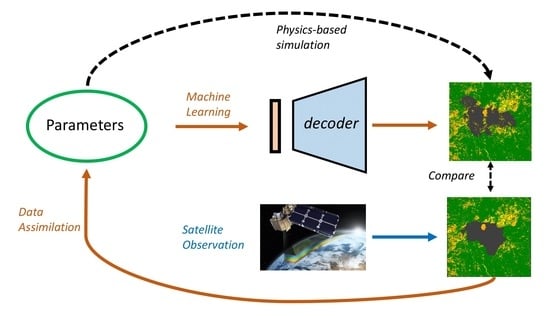
  • We propose a parameter flexible data-driven algorithm scheme for burned area forecasting which can combine different approaches of ROM and ML prediction techniques with a large range of model parameters.
  • We develop an inverse model to address the bottleneck of parameter identification in fire prediction models by using the recently developed GLA algorithm,
  • We test the parameter flexible data-driven model and the inverse model for recent massive fire events in California where the data used for the assimilation are satellite observations (ORNL DAAC. 2018. MODIS and VIIRS Land Products Global Subsetting and Visualization Tool. ORNL DAAC, Oak Ridge, Tennessee, USA) of burned area.
The resulting data-driven wildfire model with identified parameters allows fire propagation to be predicted in near-real time, which makes it suitable for use in the context of emergency response and fire fighting.

2. Data Generation and Study Area

In this section we describe the models employed to generate the data used to train the parameter flexible data-driven model for burned area forecasting, and provide information on the study area and the satellite observations.

2.1. Cellular Automata Fire Simulation

We make use of an operational CA model [7], for generating the training and testing data. The performance of this CA model was originally tested by predicting the Spetses fire in 1990 in Greece [7]. The model uses square meshes to simulate the random spatial spread of wildfires as shown in Figure 1. The use of regular square meshes reduces the computational cost for large fire events compared to using unstructured meshes. Four states are assigned to represent a cell at a discrete time:
  • state 1: the cell can not be burned;
  • state 2: the cell is burnable but has not been ignited;
  • state 3: the cell is burning;
  • state 4: the cell has been burned.
At each discrete time step, fire propagation into neighbour cells (i.e., state 3 state 4 ) is stochastic, following the probability,
P bun = p h ( 1 + p veg ) ( 1 + p den ) p s p w
where p h is the burning probability. p veg , p den , p s and p w are related to the local canopy density, canopy cover, landscape slope and wind speed/direction of the receiving cell, respectively. The actual values of these physical fields for corresponding areas were obtained from the Interagency Fuel Treatment Decision Support System [45]. The slope effect p s is modelled following [46], that is,
p s = exp ( a θ s ) .
where a is a dimensionless constant that can be adjusted. The slope angle θ s in the CA modelling [7] is calculated by:
θ s = tan 1 E 1 E 2 l for adjacent cells tan 1 E 1 E 2 2 l for diagonal cells
where E 1 and E 2 are the altitude of the cells and l is the cell length. To integrate the wind effect, we adapt the modelling in [7], that is,
p w = exp ( c 1 V w ) f t , f t = exp ( V w c 2 ( c o s ( θ w ) 1 ) )
where V w denotes the wind speed in m / s and θ w represents the angle between the wind direction and the potential fire spread direction as illustrated in Figure 1. c 1 and c 2 are two tunable coefficients of wind effect. Spotting, i.e., fire starts beyond the fire edge due to wind-transport of flaming embers, is also considered [7]. The wind data of the corresponding area and date for different fire events were extracted from the dataset of [47]. Wind speed and direction are considered as spatially constant over the 27 km × 27 km grid cell, as shown in Figure 1. The time step of the CA simulation is roughly equivalent to 30 min. To be exact, 40 CA steps are equivalent to 24 h in real time [27].
The operational parameters p h , a , c 1 , c 2 can have a large impact on the fire forecast. In [7], these parameters are fixed as
p h = 0.58 , a = 0.078 , c 1 = 0.045 , c 2 = 0.131 ,
resulting from the minimisation of a cost function that fits the observations in the specific fire event modelled. These values are used as initial guess in the parameter identification algorithm.

2.2. Study Area and Observation Data

We evaluate the performance of our modelling approaches using two recent massive fire events in California, namely the Chimney fire in 2016, and the Ferguson fire at 2018 (Table 1). The vegetation density in the area of the Chimney fire was higher than that in the Ferguson fire, resulting in a much faster rate of propagation. Thus, the two fires provide contrasting behaviour and thus a good basis for assessing the robustness of our modelling. The area indicated in Table 1 represents the study area of both fire events, which is different from the total burned area. The averaged wind speed (mph, meters per hour) for the first 6 days is also indicated for both fire events. We use active fire data generated from Moderate Resolution Imaging Spectroradiometer (MODIS) and Visible Infrared Imaging Radiometer Suite (VIIRS) satellites. MODIS provides thermal observations globally four times a day (Terra at 10:30 and 22:30; Aqua at 13:30 and 01:30 local time) at a resolution of about 1 km [48]. VIIRS thermal data provides improved fire detection capabilities every 12 h (at 13:30 and 1:30 local time) [49]. In this study, the level 2 VIIRS I-band active fire product (VNP14IMG) with a resolution of 375 m is combined with the MODIS fire products (MOD14 and MYD14) at 1 km to derive continuous daily fire perimeters, using the natural neighbour geospatial interpolation method [50]. Both MODIS and VIIRS data are available 2.5 h after the observations time, allowing near real-time fire updating.

3. A Parameter Flexible Data-Driven Model for Burned Area Forecasting: Methodology

In this section we describe the models we designed based on existing algorithms for developing a parameter flexible data-driven model for burned area forecasting, specifically the models for compressing/reducing the data, the predictive models in the low-dimensional space and the LA approach for parameter estimation.

3.1. Reduced-Order Modelling

The CA model provides a source of time series data which is used to train the ML predictive models. The size of the final dataset mandates the use of ROM techniques. To build a low dimensional latent space for burned area with high accuracy of reconstruction after decoding/decompression, we integrate and compare three different compression approaches. The burned area in the full space (obtained from simulators or satellite observations) and the encoded low-dimensional space at time t is denoted as y t and y ˜ t respectively.

3.1.1. Principle Component Analysis

We first apply the PCA method for encoding the physical fields of burned areas. A set of n y simulated fields { y t ( i ) } { i = 0 n y } at a fixed time t are flattened and combined in a matrix,
Y t = y t ( 0 ) | y t ( 1 ) | | y t ( n y ) .
In this study, n y represents the number of different sets of model parameters, which will generate different burned areas at time t through the CA modelling. The ROMs at different time steps are performed individually. For the sake of simplicity, we adopt the notation y , Y for y t , Y t in the rest of Section 3.1. We compute and decompose the empirical covariance C y ,
C y = 1 n y 1 Y Y T = L Y D Y L Y T .
Here, each column of L Y is a principal component (PC) of C y and D Y is a diagonal matrix formed by the associated eigenvalues { λ Y , i , i = 0 , , n y 1 } in decreasing order, i.e.,
D Y = λ Y , 0 λ Y , n y 1 .
A projection matrix L Y , q of truncation parameter q ( 1 q n y ) is constructed by extracting the q first columns in L Y . For each flattened field y , the PCA-encoded latent vector y ˜ is obtained via
y ˜ = L Y , q T y .
An approximation of the full field vector can be computed through PCA-decoding,
y PCA = L Y , q y ˜ = L Y , q L Y , q T y .

3.1.2. Convolutional Autoencoding

Autoencoding is an unsupervised DL approach that learns how to perform efficient data compression from the training dataset. A typical autoencoder consists of an encoder E which compresses the input vector to the latent variables and a decoder D to reconstruct the data back from the low-dimensional representation, i.e.,
y ˜ = E ( y ) and y CAE = D ( y ˜ ) .
Both encoders and decoders can be constructed via Neural Network (NNs), but this is problematic for high-dimensional data because of the large number of parameters. Furthermore, NNs treat all input variable similarly causing difficulties in representing local image features. CAE overcomes these problems by using convolutional layers in the NN structure. Convolutional layers make use of multi-dimensional filters to capture local patterns. The size of the filter is fixed in each convolutional layer. Pooling layers are then added to reduce the dimension (i.e., number of neurons). When decoding, Upsampling layers can be used to reconstruct the NN input. For more details about Convolutional Neural Network (CNN) and CAE, interested readers are referred to [51]. CAE requires training of fewer parameters and recognizes spatial patterns thanks to multi-dimensional filters. We train the convolutional encoder and decoder jointly using the mean square error (MSE) loss function,
J ( E , D ) = 1 N train j = 1 N train | | y j D E ( y j ) | | 2 .

3.1.3. Singular Value Decomposition Autoencoding

Since training a CAE is time consuming for high dimensional problems, we implement a training-efficient autoencoder, known as SVD AE or POD AE, which combines the PCA approach and the ML-based AE. Dimension reduction is performed in two steps. PCA is first applied to obtain the full set of PCs of the dynamical system, followed by a dense autoencoder ( E , D ) with fully connected layers to reduce the system dimensions further,
y ˜ = E L Y T y , while y SVD AE = L Y D ( y ˜ ) .
Thus, both the input and the ouput of the encoder E and the decoder D are the principle components of the full system. Combining PCA and ML autoencoding means this approach has both the efficiency of PCA and the power of CAE for dealing with chaotic systems. SVD AE can handle data with both structured or unstructured geometry.

3.2. Forward Problem: Machine Learning Prediction

We implement different ML regression approaches to predict the latent variables y ˜ t at different time steps using model parameters x = [ c 1 , c 2 , p h , a ] , i.e.,
y ˜ t = f t ML ( x ) .
Training is performed on an ensemble of perturbed parameter sets, generated via Latin Hypercube Sampling (LHSs) within the range,
p h [ 0.00 , 0.70 ] , a [ 0.00 , 0.14 ] , c 1 [ 0.00 , 0.12 ] , c 2 [ 0.00 , 0.40 ] ,
based on the parameter values given in the literature and some preliminary experimentation. We generated a 2300-member ensemble (i.e., 2300 simulations with different model parameters), which was then split into training and testing datasets of 1000 members and a 300-member validation dataset. The training and the testing datasets are used for both fire events, and the two fire events were simulated via CA until 8 days after the ignition.

3.2.1. Random Forest Regression

We first use random decision forests RF model, an ensemble ML approach based on Decision Tree (DTs), to predict the latent variables derived from ROM. RFs employ a bagging approach, which trains a set of individual prediction models simultaneously using a random subset of the training data. The number of individual models n DT , the maximum depth d DT of each DT and the number of features n features considered for the tree split are hyperparameters in RFs modelling and obtained based on hyperparameter tuning on the validation dataset. Here, we use Classification And Regression Tree (CART) with gini coefficients [52] for tree splitting in the DT framework.

3.2.2. K-Nearest Neighbours Regression

We also use KNN for latent variable prediction. KNN is a non-parametric machine learning method where the model outputs only depend on the k local training samples (denoted as N k ( x ) ) which are the closest to the input vector x . As a consequence, the function is only approximated by local samples and no pre-training is required. The weight of each training sample x i (for x i N k ( x ) ) is proportional to the inverse of the L 2 distance, i.e.,
y = x i N k ( x ) w i y i , where w i = 1 | | x x i | | 2 x j N k ( x ) 1 | | x x j | | 2 .
To search the ensemble of nearest samples (i.e., N k ( x ) ), we use the k d - t r e e algorithm [53] which is appropriate for low-dimensional data (here, dim ( x ) = 4 ). The maximum leaf size of the k d - t r e e is fixed as 30.

3.2.3. Multi Layer Perceptron

We also apply a deep learning (MLP) approach in the latent space to predict the fire propagation. Since the problem is of a relatively small dimension (i.e., dim ( x ) = 4 and dim ( y ) 50 ), a fully-connected NN structure with two hidden layers is employed, that is,
dim ( x ) = 4 n MLP , 1 n MLP , 2 dim ( y ) ,
where n MLP , 1 and n MLP , 2 denote the number of neurons in both hidden layers, respectively. The pipeline of the forward modelling, involving data generating, ROM, and prediction in the latent space is illustrated in Figure 2.

3.3. Inverse Problem: Latent Data Assimilation

The choice of model parameters significantly impacts the fire spread forecast. Thus, parameter calibration using real-time observations is crucial for both physics- and ML-based prediction models. We develop a novel parameter identification method based on the GLA algorithm with time-variant observations to solve the inverse problem. To reduce the computational burden, the observations are first encoded into low-dimensional latent spaces.

3.3.1. Four Dimensional Variational Approach

We employ data assimilation for model parameter identification by fitting the encoded observations { y ˜ t } within an observing window T obs = { t 1 , , t n o b s } by implementing 4Dvar algorithm [44] using the ML forward models and defining the loss function as:
J ( x ) = 1 2 | | x x b | | B 1 2 + 1 2 t T obs | | y ˜ t f t ML ( x ) | | R t ˜ 1 2
where B , R ˜ t represent the prior error covariance matrices [54,55] associated to the states and encoded observations, respectively. These covariance matrices are set to be diagonal in the latent space in this study. Minimising the 4Dvar loss function (Equation (18)) leads to the analysis state,
x a = argmin x J ( x ) .
The minimisation of 4Dvar is performed using the LBFGS approach [56], where each minimisation iteration can be written as:
x ( k + 1 ) = x ( k ) l rate Hessian ( J ) x k 1 J ( x ( k ) ) .
Here, k is the current iteration number and l rate > 0 is the learning rate of the descent algorithm.
Hessian J ( x = [ x 0 , , x n x 1 ] ) i , j = 2 J x i x j
is the Hessian matrix of the cost function J . The computation of Hessian ( J ) is thus required for implementing variational assimilation.

3.3.2. Generalised Latent Assimilation

Since the model parameters and the encoded observations y ˜ t are mapped through ML functions, the direct computation of Hessian ( J ) can be difficult due to the high non-linearity and the large number of model parameters. The recent work of [41] proposed a new assimilation approach GLA to tackle this bottleneck in current Latent Assimilation methods, where local Polynomial Regression (PRs) are performed in a neighbourhood of the background state to build a smooth local surrogate function to facilitate the computation of the Hessian matrix in the optimisation loops. Here, LHS is performed to build a PR learning ensemble { x b q } q = 1 . . n s around the background state within certain range r s (i.e., sampling from [ ( 1 ± r s ) x 0 , , ( 1 ± r s ) x n x 1 ] ). We then fit the ML model output by a local polynomial function H ˜ t p , i.e.,
H ˜ t p = argmin P P ( d p ) ( q = 1 n s | | p ( x b q ) f t ML ( x b q ) | | 2 2 ) 1 / 2 ,
where P ( d p ) represents the set of polynomial functions of degree d p . { d p , n s , r s } are considered as hyperparamters of the algorithm. We extend the GLA to a 4Dvar framework with time-dependent observations, as shown in Algorithm 1.
Once the analysis state (i.e., assimilated parameters) x a is obtained, forecasts of future burned area at time t can be made,
y t pred = D y f t ML ( x a ) .
The pipeline of the inverse modelling for parameter estimation is illustrated in Figure 3.   
Algorithm 1: 4Dvar GLA
Remotesensing 14 03228 i001

3.4. Hyperparameter Tuning

To select the most appropriate data compression methods, we apply the three different ROM approaches and evaluate their performance on the unseen test dataset and satellite observations. Forward models are trained on simulated burned areas individually 2, 4, 6 days after the ignition of each fire in order to capture the time of the fastest propagation. We set the burned and burning cells to 1 while unburned cells are set to 0. A threshold of 0.5 is set to classify the output cells after reconstruction to the full space. The performance of different ROMs and prediction models is evaluated using both the test dataset (obtained via CA simulations) and the satellite observations. Hyperparameter tuning is carried out for both the forward and inverse models on the validation dataset as shown in Table 2. For both fire events, the NN structures of CAE and SVD AE are similar. The exact networks for the Chimney fire are shown as an example in Table 3.

4. Results and Analysis

In this section, we present and analyse the numerical results from ROM, ML forecasting and GLA parameter estimation using simulated data and satellite observations.

4.1. Reconstruction Accuracy of Reduced Order Modellings

To compare different ROMs, we compute the relative reconstruction error after decoding,
ϵ rec = | | y y { PCA , CAE , SVD AE } | | 1 dim ( y ) ,
where | | . | | 1 denotes the one-norm, in other words, the number of mis-predicted pixels. With the same number of latent variables for different ROMs, ϵ rec represents the efficiency of data compression strategies which is crucial for predictions latter. The evolution of ϵ rec against the truncation parameter (i.e., the dimension of the latent space) is shown in Figure 4 for both the Chimney and the Ferguson fire events at both the day 2 and the day 4. The estimation of ϵ rec was made using all 1000 simulations in the test dataset of CA simulations (Figure 4a,c) while the ϵ rec for the real fire (Figure 4b,d) is evaluated using the satellite observation (a single image) at day 4.
Reconstruction errors increase with time from the start of the fire for both fires as shown in Figure 4b,d. The reconstruction errors for the satellite images are larger than those for the test data, which is to be expected since the autoencoders were trained entirely using simulated data. The PCA and SVD AE approaches have lower reconstruction errors than CAE in the test dataset generated by CA simulations. However, CAE shows better performance against the satellite data than either PCA or SVD AE. The differences between the three approaches are also seen in the predictions of burnt area. In Figure 5 and Figure 6, we show the reconstruction of different ROMs for two sets of model parameters where the original CA simulations are represented by sub-figures (a,i) for each fire. The PCA and SVD AE approaches are better at representing local variability in burnt area in the test dataset (Figure 5 and Figure 6f–h,n–p). However, overfitting to the CA dataset means that they are less good than CAE at predicting the satellite observations (Figure 7). On the other hand, CAE produces more continuous burned areas compared to PCA and SVD AE because of the convolutional layers in compressing and reconstructing the images. These findings are consistent with the results obtained in Figure 4 and the earlier analysis of other fire events [27]. The Ferguson fire has a higher average vegetation density, leading to a considerably faster fire spread than in the Chimney fire (Figure 5 and Figure 6). This is seen in both the CA simulations and the observations of burned area. It would be possible to improve the performance of these ML-based ROMs, particularly the CAE and SVD AE) approaches, by increasing the size of the training dataset, but this would increase the computational cost since the CA simulation is relatively slow. Because most of the ROMs achieve a stable performance for q 30 , we fix the dimension of the latent space as q = 30 for both forward and inverse modellings in the rest of this paper.

4.2. Prediction Performance of the Forward Model

Having compressed the full space of burned area into low-dimensional latent variables, we apply the models introduced in Section 3.2 to predict fire propagation in these reduced spaces using the same training, validation and test datasets as for ROMs. Comparisons of the predictions of latent variables on the test dataset against the true compressed values is illustrated in Figure 8. We focus on the most important PC (i.e., the one associated to λ Y , 0 ) for the PCA approach and the latent variables with highest variance for CAE and SVD AE. For clarity, the samples in each sub-figure are reordered in increasing order along the true compressed values (i.e., red curves). Since CA generates probabilistic simulations, the same set of model parameters may lead to different simulations of burned area which introduces some uncertainties in the ML approaches as observed in Figure 8. Nevertheless, the predictions for the test dataset are still reasonably accurate and show the advantage of DL-based approaches. We show the forecasting error ϵ pred (defined similarly to ϵ rec ) in the full space after decoding in Table 4. Good prediction accuracy (with an error below 5 % in the full space) can be achieved by each combination of ROM and ML approaches. The PCA and SVD AE approaches produce slightly more accurate predictions compared to CAE-based approaches due to the reconstruction error on the CA test dataset, as discussed in Section 4.1. The predicted burned areas using CAE are more continuous.
The training time of ML approaches (i.e., KNN, RF and MLP) in the latent space differs slightly when combined with different ROMs. As an example, we show the training time in the reduced space of CAE in Table 5. The main computational cost for online prediction is decoding, since the evaluation of trained ML algorithms is very fast. We show the results of RF coupling with different ROM approaches, but using KNN or MLP produces similar results. In Table 5, only the training of CAE is performed with one NVIDIA P100 GPU (RAM of 16 Gb) of Google Colab environment. The other works including CA, are carried out with Colab Intel CPUs (2.30 GHz and 26.75 Gb RAM). The ROM and ML-based online predictions (especially with CAE and PCA), are much faster than the physics-based CA simulations. The online prediction of SVD AE is relatively slow because its decoding involves a large number of principle components. Comparing the results in Table 4 and Table 5 and Figure 4, SVD AE is out-performed by PCA in terms of both reconstruction/prediction accuracy and online efficiency. We, therefore, only focus on PCA and CAE for parameter estimation.

4.3. Parameter Estimation of the Inverse Model

We use observations of day 2 and day 4 to improve parameter estimation following the flowchart shown in Figure 3 and test the algorithm performance for the accuracy of predictions on day 6 for both fire events. The CA simulation using the true parameters in the test dataset is considered as the ground truth. Only slight differences are found between the third and the fourth columns of Figure 9, which confirms the accuracy of the forward modelling. The predictions with assimilated parameters (i.e., CAE-MLP ( x a ) ) are much closer to the CA simulations (i.e., CA ( x t ) ) regarding the background predictions (i.e., CAE-MLP ( x b ) ) using by-default values (Equation (5)) of parameters. The strength of GLA when dealing with satellite data can be seen in Figure 10, where the preprocessed satellite images of day 2 and day 4 (Figure 7a,i) have been used as observations in GLA for parameter estimation after encoding. Since both the forward prediction models and the ROMs are trained using simulated data, their adaptation to satellite images is imperfect. Nevertheless, the GLA produces a better forecast of observed burned area (Figure 10c,h) for both CAE-MLP and PCA-MLP approaches. The predictions performed using assimilated parameters (Figure 10b,e,g,j) are much closer to the satellite observations (Figure 10c,h) regarding initial guesses (Figure 10a,d,f,i). Quantitative comparison of averaged relative error (Equation (24)) is shown in Table 6. A considerable reduction of prediction error for all combinations of ML and ROM approaches can be observed. This is coherent with our analysis of Figure 7 and Figure 10. Thus, GLA preforms well in correcting both the overestimation (Ferguson fire) and underestimation (Chimney fire) of model parameters. The predictions of future burned area of day 6 made by assimilated parameters are much closer to the observations than the predictions using prior parameters. Further more, the low computational time of GLA (evaluated on the test dataset since only one satellite observation is available for each fire at day 6), allows efficient online parameter estimation, facilitating near real-time fire assimilation/monitoring.

5. Conclusions

Current tools for dynamical wildfire forecasting are difficult to apply for real-time fire forecasting. We have developed a scheme which combines different reduced-order modellings and data-driven prediction models for efficient parameter-flexible burned area forecasting. We have extended the Latent Assimilation framework to time-variant (i.e., 4Dvar) optimisation problems. Our parameter estimation approach can be adjusted efficiently using available observation data in near real-time. The results clearly demonstrate the efficiency and the robustness of the proposed approach. The method relies on ML from physics-based CA simulations; such simulations have been successfully run for many different regions (e.g., [57,58]) and thus our approach should be generalisable to other regions and ecosystems. The system represented in this study is also data-agnostic, and could easily be applied to other dynamical systems.
Nevertheless, although the reduced-order modelling and the forward prediction methods achieved a precise reconstruction on the test dataset (also generated by the CA model), there are still difficulties in predicting real-time satellite images. Further efforts to improve the adaptive capability of the current system when dealing unseen satellite data could focus on, for instance, enhancing the regularity of autoencoding via variational autoencoders [17], online fine tuning [59] and domain adaption techniques [60]. Our approach requires individual ROMs and ML prediction models for different ecoregions, which could be computationally expensive for offline simulation and training. It may be possible to overcome this limitation, by using fire prediction models on a global scale with sparser grids, which yields a tradeoff between forecasting accuracy and generalisability. Further work to improve the forward and inverse modellings could focus on learning from more complex fire simulations, for example simulations which take into account of fuel moisture, the incidence of spotting or surface-to- crown transitions.

Author Contributions

Conceptualization, S.C. and R.A.; methodology, S.C.; software, S.C.; validation, R.A., S.P.H., I.C.P., C.Q.-C. and Y.-K.G.; formal analysis, S.C. and S.P.H.; data curation, S.C. and Y.J.; writing—original draft preparation, S.C.; writing—review and editing, S.C., S.P.H., R.A. and Y.J.; visualization, S.C.; supervision, R.A. and Y.-K.G.; project administration, I.C.P.; funding acquisition, I.C.P. and Y.-K.G. All authors have read and agreed to the published version of the manuscript.

Funding

This research is funded by the Leverhulme Centre for Wildfires, Environment and Society through the Leverhulme Trust, grant number RC-2018-023. This work is partially supported by the EP/T000414/1 PREdictive Modelling with QuantIfication of UncERtainty for MultiphasE Systems (PREMIERE).

Data Availability Statement

Data available upon reasonable request to the corresponding author.

Acknowledgments

The authors would like to thank Yuhan Huang for performing satellite data curation. The authors thank the anonymous reviewers for their careful reading of our manuscript and their many insightful comments and suggestions.

Conflicts of Interest

The authors declare no conflict of interest.

Acronyms

NNNeural Network
DNNDeep Neural Network
MLMachine Learning
LALatent Assimilation
DAData Assimilation
PRPolynomial Regression
AEAutoencoder
VAEVariational Autoencoder
CAEConvolutional Autoencoder
VAEVariational Autoencoder
BLUEBest Linear Unbiased Estimator
3D-Var3D Variational
RNNRecurrent Neural Network
CNNConvolutional Neural Network
LSTMlong short-term memory
PODProper Orthogonal Decomposition
PCAPrincipal Component Analysis
PCprincipal component
SVDSingular Value Decomposition
ROMreduced-order modelling
CFDcomputational fluid dynamics
1Done-dimensional
2Dtwo-dimensional
NWPnumerical weather prediction
MSEmean square error
S2Ssequence-to-sequence
R-RMSErelative root mean square error
BFGSBroyden–Fletcher–Goldfarb–Shanno
LHSLatin Hypercube Sampling
AIartificial intelligence
DLDeep Learning
PIVParticle Image Velocimetry
LIFLaser Induced Fluorescence
KNNK-nearest Neighbours
DTDecision Tree
RFRandom Forest
KFKalman filter
CARTClassification And Regression Tree
CACellular Automata
MLPMulti Layer Percepton
GLAGeneralised Latent Assimilation
3DvarThree-dimensional variational data assimilation
4DvarFour-dimensional variational data assimilation
MODISModerate Resolution Imaging Spectroradiometer
VIIRSVisible Infrared Imaging Radiometer Suite

References

  1. Chen, G.; Guo, Y.; Yue, X.; Tong, S.; Gasparrini, A.; Bell, M.L.; Armstrong, B.; Schwartz, J.; Jaakkola, J.J.; Zanobetti, A.; et al. Mortality risk attributable to wildfire-related PM2· 5 pollution: A global time series study in 749 locations. Lancet Planet. Health 2021, 5, e579–e587. [Google Scholar] [CrossRef]
  2. Verisk Wildfire Risk Analysis: Number of Properties at High to Extreme Risk; Wildfire: Redwood City, CA, USA, 2021.
  3. Hanson, H.P.; Bradley, M.M.; Bossert, J.E.; Linn, R.R.; Younker, L.W. The potential and promise of physics-based wildfire simulation. Environ. Sci. Policy 2000, 3, 161–172. [Google Scholar] [CrossRef]
  4. Viegas, D.X.; Simeoni, A. Eruptive behaviour of forest fires. Fire Technol. 2011, 47, 303–320. [Google Scholar] [CrossRef] [Green Version]
  5. Valero, M.M.; Jofre, L.; Torres, R. Multifidelity prediction in wildfire spread simulation: Modeling, uncertainty quantification and sensitivity analysis. Environ. Model. Softw. 2021, 141, 105050. [Google Scholar] [CrossRef]
  6. Maffei, C.; Menenti, M. Predicting forest fires burned area and rate of spread from pre-fire multispectral satellite measurements. ISPRS J. Photogramm. Remote Sens. 2019, 158, 263–278. [Google Scholar] [CrossRef]
  7. Alexandridis, A.; Vakalis, D.; Siettos, C.; Bafas, G. A cellular automata model for forest fire spread prediction: The case of the wildfire that swept through Spetses Island in 1990. Appl. Math. Comput. 2008, 204, 191–201. [Google Scholar] [CrossRef]
  8. Papadopoulos, G.D.; Pavlidou, F.N. A comparative review on wildfire simulators. IEEE Syst. J. 2011, 5, 233–243. [Google Scholar] [CrossRef]
  9. Casas, C.Q.; Arcucci, R.; Wu, P.; Pain, C.; Guo, Y.K. A Reduced Order Deep Data Assimilation model. Phys. D Nonlinear Phenom. 2020, 412, 132615. [Google Scholar] [CrossRef]
  10. Murata, T.; Fukami, K.; Fukagata, K. Nonlinear mode decomposition with convolutional neural networks for fluid dynamics. J. Fluid Mech. 2020, 882. [Google Scholar] [CrossRef] [Green Version]
  11. Ravuri, S.; Lenc, K.; Willson, M.; Kangin, D.; Lam, R.; Mirowski, P.; Fitzsimons, M.; Athanassiadou, M.; Kashem, S.; Madge, S.; et al. Skilful precipitation nowcasting using deep generative models of radar. Nature 2021, 597, 672–677. [Google Scholar] [CrossRef]
  12. Gong, H.; Cheng, S.; Chen, Z.; Li, Q. Data-Enabled Physics-Informed Machine Learning for Reduced-Order Modeling Digital Twin: Application to Nuclear Reactor Physics. Nucl. Sci. Eng. 2022, 196, 668–693. [Google Scholar] [CrossRef]
  13. Fukami, K.; Murata, T.; Zhang, K.; Fukagata, K. Sparse identification of nonlinear dynamics with low-dimensionalized flow representations. J. Fluid Mech. 2021, 926, A10. [Google Scholar] [CrossRef]
  14. Hinze, M.; Volkwein, S. Proper orthogonal decomposition surrogate models for nonlinear dynamical systems: Error estimates and suboptimal control. In Dimension Reduction of Large-Scale Systems; Springer: Berlin/Heidelberg, Germany, 2005; pp. 261–306. [Google Scholar]
  15. Cheng, S.; Lucor, D.; Argaud, J.P. Observation data compression for variational assimilation of dynamical systems. J. Comput. Sci. 2021, 53, 101405. [Google Scholar] [CrossRef]
  16. Guo, Y.; Liu, Y.; Oerlemans, A.; Lao, S.; Wu, S.; Lew, M.S. Deep learning for visual understanding: A review. Neurocomputing 2016, 187, 27–48. [Google Scholar] [CrossRef]
  17. Pu, Y.; Gan, Z.; Henao, R.; Yuan, X.; Li, C.; Stevens, A.; Carin, L. Variational autoencoder for deep learning of images, labels and captions. Adv. Neural Inf. Process. Syst. 2016, 29, 1–9. [Google Scholar]
  18. Phillips, T.R.; Heaney, C.E.; Smith, P.N.; Pain, C.C. An autoencoder-based reduced-order model for eigenvalue problems with application to neutron diffusion. Int. J. Numer. Methods Eng. 2021, 122, 3780–3811. [Google Scholar] [CrossRef]
  19. Quilodrán-Casas, C.; Arcucci, R.; Mottet, L.; Guo, Y.; Pain, C. Adversarial autoencoders and adversarial LSTM for improved forecasts of urban air pollution simulations. arXiv 2021, arXiv:2012.12056. [Google Scholar]
  20. Pache, R.; Rung, T. Data-driven surrogate modeling of aerodynamic forces on the superstructure of container vessels. Eng. Appl. Comput. Fluid Mech. 2022, 16, 746–763. [Google Scholar] [CrossRef]
  21. Ly, H.; Tran, H. Modeling and control of physical processes using proper orthog- onal decomposition. J. Math. Comput. Model 2001, 33, 223–236. [Google Scholar] [CrossRef] [Green Version]
  22. Xiao, D.; Du, J.; Fang, F.; Pain, C.; Li, J. Parameterised non-intrusive reduced order methods for ensemble Kalman filter data assimilation. Comput. Fluids 2018, 177, 69–77. [Google Scholar] [CrossRef]
  23. Xiao, D.; Fang, F.; Pain, C.; Navon, I. A parameterized non-intrusive reduced order model and error analysis for general time-dependent nonlinear partial differential equations and its applications. Comput. Methods Appl. Mech. Eng. 2017, 317, 868–889. [Google Scholar] [CrossRef] [Green Version]
  24. Audouze, C.; Vuyst, F.D.; Nair, P.B. Reduced-order modeling of parameterized PDEs using time-space-parameter principal component analysis. Int. J. Numer. Methods Eng. 2009, 80, 1025–1057. [Google Scholar] [CrossRef]
  25. Xiao, D.; Yang, P.; Fang, F.; Xiang, J.; Pain, C.C.; Navon, I.M. Non-intrusive reduced order modelling of fluid–structure interactions. Comput. Methods Appl. Mech. Eng. 2016, 303, 35–54. [Google Scholar] [CrossRef] [Green Version]
  26. Liu, C.; Fu, R.; Xiao, D.; Stefanescu, R.; Sharma, P.; Zhu, C.; Sun, S.; Wang, C. EnKF data-driven reduced order assimilation system. Eng. Anal. Bound. Elem. 2022, 139, 46–55. [Google Scholar] [CrossRef]
  27. Cheng, S.; Prentice, I.C.; Huang, Y.; Jin, Y.; Guo, Y.K.; Arcucci, R. Data-driven surrogate model with latent data assimilation: Application to wildfire forecasting. J. Comput. Phys. 2022, 464, 111302. [Google Scholar] [CrossRef]
  28. Finney, M.A. FARSITE, Fire Area Simulator—Model Development and Evaluation; Number 4; US Department of Agriculture, Forest Service, Rocky Mountain Research Station: Fort Collins, CO, USA, 1998. [Google Scholar]
  29. Hilton, J.E.; Sullivan, A.L.; Swedosh, W.; Sharples, J.; Thomas, C. Incorporating convective feedback in wildfire simulations using pyrogenic potential. Environ. Model. Softw. 2018, 107, 12–24. [Google Scholar] [CrossRef]
  30. Mallet, V.; Keyes, D.E.; Fendell, F. Modeling wildland fire propagation with level set methods. Comput. Math. Appl. 2009, 57, 1089–1101. [Google Scholar] [CrossRef] [Green Version]
  31. Mu noz-Esparza, D.; Kosović, B.; Jiménez, P.A.; Coen, J.L. An accurate fire-spread algorithm in the Weather Research and Forecasting model using the level-set method. J. Adv. Model. Earth Syst. 2018, 10, 908–926. [Google Scholar] [CrossRef] [Green Version]
  32. Ambroz, M.; Mikula, K.; Fraštia, M.; Marčiš, M. Parameter estimation for the forest fire propagation model. Tatra Mt. Math. Publ. 2018, 75, 1–22. [Google Scholar] [CrossRef]
  33. Lautenberger, C. Wildland fire modeling with an Eulerian level set method and automated calibration. Fire Saf. J. 2013, 62, 289–298. [Google Scholar] [CrossRef]
  34. Rochoux, M.; Emery, C.; Ricci, S.; Cuenot, B.; Trouvé, A. A comparative study of parameter estimation and state estimation approaches in data-driven wildfire spread modeling. In Proceedings of the VII International Conference on Forest Fire Research, Coimbra, Portugal, 17–20 November 2014; pp. 14–20. [Google Scholar]
  35. Ervilha, A.; Pereira, J.; Pereira, J. On the parametric uncertainty quantification of the Rothermel’s rate of spread model. Appl. Math. Model. 2017, 41, 37–53. [Google Scholar] [CrossRef]
  36. Zhang, C.; Collin, A.; Moireau, P.; Trouvé, A.; Rochoux, M.C. State-parameter estimation approach for data-driven wildland fire spread modeling: Application to the 2012 RxCADRE S5 field-scale experiment. Fire Saf. J. 2019, 105, 286–299. [Google Scholar] [CrossRef]
  37. Alessandri, A.; Bagnerini, P.; Gaggero, M.; Mantelli, L. Parameter estimation of fire propagation models using level set methods. Appl. Math. Model. 2021, 92, 731–747. [Google Scholar] [CrossRef]
  38. Jensen, C.A.; Reed, R.D.; Marks, R.J.; El-Sharkawi, M.A.; Jung, J.B.; Miyamoto, R.T.; Anderson, G.M.; Eggen, C.J. Inversion of feedforward neural networks: Algorithms and applications. Proc. IEEE 1999, 87, 1536–1549. [Google Scholar] [CrossRef]
  39. Amendola, M.; Arcucci, R.; Mottet, L.; Casas, C.Q.; Fan, S.; Pain, C.; Linden, P.; Guo, Y.K. Data Assimilation in the Latent Space of a Neural Network. arXiv 2020, arXiv:2104.06297. [Google Scholar]
  40. Peyron, M.; Fillion, A.; Gürol, S.; Marchais, V.; Gratton, S.; Boudier, P.; Goret, G. Latent space data assimilation by using deep learning. Q. J. R. Meteorol. Soc. 2021, 147, 3759–3777. [Google Scholar] [CrossRef]
  41. Cheng, S.; Chen, J.; Anastasiou, C.; Angeli, P.; Matar, O.K.; Guo, Y.K.; Pain, C.C.; Arcucci, R. Generalised Latent Assimilation in Heterogeneous Reduced Spaces with Machine Learning Surrogate Models. arXiv 2022, arXiv:2204.03497. [Google Scholar]
  42. Carrassi, A.; Bocquet, M.; Bertino, L.; Evensen, G. Data assimilation in the geosciences: An overview of methods, issues, and perspectives. Wiley Interdiscip. Rev. Clim. Chang. 2018, 9, e535. [Google Scholar] [CrossRef] [Green Version]
  43. Cheng, S.; Argaud, J.P.; Iooss, B.; Lucor, D.; Ponçot, A. Background error covariance iterative updating with invariant observation measures for data assimilation. Stoch. Environ. Res. Risk Assess. 2019, 33, 2033–2051. [Google Scholar] [CrossRef] [Green Version]
  44. Ide, K.; Courtier, P.; Ghil, M.; Lorenc, A.C. Unified notation for data assimilation: Operational, sequential and variational (gtspecial issueltdata assimilation in meteology and oceanography: Theory and practice). J. Meteorol. Soc. Jpn. Ser. II 1997, 75, 181–189. [Google Scholar] [CrossRef] [Green Version]
  45. Drury, S.A.; Rauscher, H.M.; Banwell, E.M.; Huang, S.; Lavezzo, T.L. The interagency fuels treatment decision support system: Functionality for fuels treatment planning. Fire Ecol. 2016, 12, 103–123. [Google Scholar] [CrossRef] [Green Version]
  46. Weise, D.R.; Biging, G.S. A qualitative comparison of fire spread models incorporating wind and slope effects. For. Sci. 1997, 43, 170–180. [Google Scholar]
  47. Hersbach, H. Copernicus Climate Change Service (C3S) (2017): ERA5: Fifth Generation of ECMWF Atmospheric Reanalyses of the Global Climate; Technical Report; Copernicus Climate Change Service Climate Data Store (CDS); ACM: New York, NY, USA, 2017. [Google Scholar]
  48. Giglio, L.; Schroeder, W.; Justice, C.O. The collection 6 MODIS active fire detection algorithm and fire products. Remote Sens. Environ. 2016, 178, 31–41. [Google Scholar] [CrossRef] [Green Version]
  49. Schroeder, W.; Oliva, P.; Giglio, L.; Csiszar, I.A. The New VIIRS 375 m active fire detection data product: Algorithm description and initial assessment. Remote Sens. Environ. 2014, 143, 85–96. [Google Scholar] [CrossRef]
  50. Scaduto, E.; Chen, B.; Jin, Y. Satellite-Based Fire Progression Mapping: A Comprehensive Assessment for Large Fires in Northern California. IEEE J. Sel. Top. Appl. Earth Obs. Remote Sens. 2020, 13, 5102–5114. [Google Scholar] [CrossRef]
  51. Rawat, W.; Wang, Z. Deep convolutional neural networks for image classification: A comprehensive review. Neural Comput. 2017, 29, 2352–2449. [Google Scholar] [CrossRef]
  52. Lewis, R.J. An introduction to classification and regression tree (CART) analysis. In Proceedings of the Annual Meeting of the Society for Academic Emergency Medicine, San Francisco, CA, USA, 22–25 May 2000; Volume 14. [Google Scholar]
  53. Ram, P.; Sinha, K. Revisiting kd-tree for nearest neighbor search. In Proceedings of the 25th ACM Sigkdd International Conference on Knowledge Discovery & Data Mining, Anchorage, AK, USA, 4–8 August 2019; pp. 1378–1388. [Google Scholar]
  54. Tandeo, P.; Ailliot, P.; Bocquet, M.; Carrassi, A.; Miyoshi, T.; Pulido, M.; Zhen, Y. A Review of Innovation-Based Methods to Jointly Estimate Model and Observation Error Covariance Matrices in Ensemble Data Assimilation. arXiv 2018, arXiv:1807.11221. [Google Scholar] [CrossRef]
  55. Cheng, S.; Qiu, M. Observation error covariance specification in dynamical systems for data assimilation using recurrent neural networks. Neural Comput. Appl. 2021, 1–19. [Google Scholar] [CrossRef]
  56. Fulton, W. Eigenvalues, invariant factors, highest weights, and Schubert calculus. Bull. Am. Math. Soc. 2000, 37, 209–250. [Google Scholar] [CrossRef] [Green Version]
  57. Trucchia, A.; D’Andrea, M.; Baghino, F.; Fiorucci, P.; Ferraris, L.; Negro, D.; Gollini, A.; Severino, M. PROPAGATOR: An operational cellular-automata based wildfire simulator. Fire 2020, 3, 26. [Google Scholar] [CrossRef]
  58. Freire, J.G.; DaCamara, C.C. Using cellular automata to simulate wildfire propagation and to assist in fire management. Nat. Hazards Earth Syst. Sci. 2019, 19, 169–179. [Google Scholar] [CrossRef] [Green Version]
  59. Devlin, J.; Chang, M.W.; Lee, K.; Toutanova, K. Bert: Pre-training of deep bidirectional transformers for language understanding. arXiv 2018, arXiv:1810.04805. [Google Scholar]
  60. Peng, X.; Huang, Z.; Zhu, Y.; Saenko, K. Federated adversarial domain adaptation. arXiv 2019, arXiv:1911.02054. [Google Scholar]
Figure 1. Wind effect in the CA modelling.
Remotesensing 14 03228 g001
Figure 2. Flowchart of the forward prediction model with CA and ROM for a specific ecoregion. The data generation is performed with a set of parameters perturbed using LHS.
Remotesensing 14 03228 g002
Figure 3. Flowchart of the inverse model for parameter identification using GLA.
Remotesensing 14 03228 g003
Figure 4. Relative reconstruction error of satellite observations and CA simulations in the test dataset against the dimension of the latent space.
Remotesensing 14 03228 g004
Figure 5. Reconstruction of CA simulations for 2 examples in the test dataset of the Chimney fire at day 4.
Remotesensing 14 03228 g005
Figure 6. Reconstruction of CA simulations for 2 examples in the test dataset of the Ferguson fire at day 4.
Remotesensing 14 03228 g006
Figure 7. Reconstruction of the satellite observation for the Chimney (ah) and the Ferguson (ip) fire at day 4.
Remotesensing 14 03228 g007
Figure 8. Prediction results of latent variables (with the highest variance in each case) for q = 30 in the test dataset for both Chimney (C) and Ferguson (F) wildfires at day 4. The x-axis represents reordered samples according to their true latent values.
Remotesensing 14 03228 g008aRemotesensing 14 03228 g008b
Figure 9. Machine learning (DL) prediction of burned area at day 6 for both fire events (Chimney (ah) and Ferguson (ip)) using original ( x b ) and assimilated ( x a ) parameters compared to CA simulations (considered as ground truth here) for 2 examples in the test dataset.
Remotesensing 14 03228 g009aRemotesensing 14 03228 g009b
Figure 10. Machine learning (DL) prediction of burned area at day 6 for both fire events using original ( x b ) and assimilated ( x a ) parameters compared to satellite observations. The results of both CAE-MLP (a,b,f,g) and PCA-MLP (d,e,i,j) are demonstrated.
Remotesensing 14 03228 g010aRemotesensing 14 03228 g010b
Table 1. Study areas of the Chimney and the Ferguson wildfire events in this work. The latitude and the longtitude represent the centre of the fires. The averaged wind speed of the first 6 days of fire propagation is also indicated.
FireLatitudeLongitudeAreaDurationStartWind
Chimney37.6230−119.8247 246 km 2 23 days13 August 201623.56 mph
Ferguson35.7386−121.0743 185 km 2 36 dyas13 July 201818.54 mph
Table 2. Hyperparameter grid search space.
Model/HyperparametersGrid Search SpaceFinal Set
CAE
Filter, Strides, Pooling size/Table 3
Activation{ReLu, LeakyReLu, Sigmoid}Table 3
Optimizer{Adam, SGD}Adam
Batch size { 16 , 32 , 64 } 32
RF
split criteria{‘gini’, ‘entropy’}‘gini’
n DT { 10 , 50 , 100 } 100
n features {‘log2’, ‘sqrt’}‘sqrt’
KNN
k{5, 10, 20}5
Metric { L 1 , L 2 } L 2
MLP
n MLP , 1 {10, 20, 30}20
n MLP , 2 {30, 40, 50}30
Activation{ReLu, LeakyReLu, Sigmoid}
Optimizer{Adam, SGD}Adam
GLA
d p 2–64
n s { 200 , 500 , 1000 , 2000 } 1000
r s 50–200% 80 %
Table 3. NN structure of the CAE with ordered meshes where the latent dimension q { 10 , 20 , 30 , 40 , 50 } .
Layer (Type)Output ShapeActivation
Encoder
Input ( 899 , 982 , 1 )
Conv 2D (10 × 10) ( 899 , 982 , 4 ) ReLu
MaxPooling 2D (5 × 5) ( 180 , 197 , 4 )
Conv 2D (4 × 4) ( 180 , 197 , 4 ) ReLu
MaxPooling 2D (3 × 3) ( 60 , 66 , 8 )
Conv 2D (3 × 3) ( 60 , 66 , 8 ) ReLu
MaxPooling 2D (3 × 3) ( 20 , 22 , 8 )
Conv 2D (2 × 2) ( 20 , 22 , 8 ) ReLu
MaxPooling 2D (2 × 2) ( 10 , 11 , 8 )
Flatten880
Dense ( q ) qLeakyReLu (0.3)
Decoder
Inputq
Dense ( 110 ) 110LeakyReLu (0.3)
Reshape ( 10 , 11 , 1 )
Conv 2D (2 × 2) ( 10 , 11 , 8 ) ReLu
Upsampling 2D (2 × 2) ( 20 , 22 , 8 )
Conv 2D (3 × 3) ( 10 , 11 , 8 ) ReLu
Upsampling 2D (3 × 3) ( 60 , 66 , 8 )
Conv 2D (4 × 4) ( 60 , 66 , 8 ) ReLu
Upsampling 2D (3 × 3) ( 180 , 198 , 8 )
Conv 2D (5 × 5) ( 180 , 198 , 4 ) ReLu
Upsampling 2D (5 × 5) ( 900 , 990 , 4 )
Cropping 2D ( 1 , 8 ) ( 899 , 982 , 4 )
Conv 2D (8 × 8) ( 899 , 982 , 1 ) Sigmoid
Table 4. Averaged prediction error for Chimney and Ferguson fires at day 4 in the full physical space after decoding. The dimension of the latent space is fixed as q = 30 .
ML ApproacheChimneyFerguson
PCACAESVD AEPCACAESVD AE
KNN1.87%4.95%1.88%2.00 %3.30%2.73%
RF1.70%4.91%1.80%1.89%3.27%2.45%
MLP1.71%4.54%1.59%2.13%3.11%2.54%
Table 5. Averaged computational time for offline training (on the training dataset of 1000 samples) and online prediction(for each sample including decoding) for different ROMs using RF. The dimension of the latent space is fixed as q = 30 .
FireOffline ROM and ML TrainingOnline Prediction
PCACAESVD AEKNNRFMLPCAPCACAESVD AE
Chimney101.06 s≈1 h 38 min414.55 s0.02 s0.67 s108 s≈35 min0.52 s0.41 s14.47 s
Ferguson97.50 s≈1 h 29 min316.61 s0.02 s0.54 s116 s≈29 min0.25 s0.31 s18.62 s
Table 6. Relative prediction error and the averaged computational time (only the LA for parameter estimation) for the Chimney and the Ferguson fire at day 6 with assimilated parameters.
FireDataForwardPCACAE
PriorPosteriorTimePriorPosteriorTime
ChimneyCA(test)KNN10.1%6.0%0.98 s11.1%7.5%0.52 s
RF10.4%5.7%0.78 s10.2%6.6%0.45 s
MLP10.9%6.3%1.25 s10.6%5.0%0.46 s
observationMLP8.3%5.0% 9.65%6.5%
FergusonCA(test)KNN30.5%20.3%0.74 s21.3%9.4%0.60 s
RF27.0%22.5%0.60 s23.1%13.6%0.58 s
MLP30.7%17.9%0.76 s22.4%12.6%0.88 s
observationMLP41.6%14.8% 23.8%11.9%
Publisher’s Note: MDPI stays neutral with regard to jurisdictional claims in published maps and institutional affiliations.

